First characterization of a new perturbation system for gust generation: the chopper

We present a new system for the generation of rapid, strong flow perturbations in the aerodynamic wind tunnel at École Centrale de Nantes. The system is called the chopper, and it consists of a rotating bar cutting through the inlet of a wind tunnel test section, thus generating an inverse gust that travels downstream. The flow generated by the chopper is investigated with respect to the rotational frequency using an array equipped with hot-wires that is traversed downstream in the flow field. It is found that the gust can be described as a superposition of the mean gust velocity, an underlying gust shape, and additional turbulence. Following this approach, the evolution of the mean gust velocity and turbulence intensity are presented, and the evolution of the underlying inverse gust shape is explained. The turbulence is shown to be characterized by an integral length scale of approximately half the chopper blade width and a turbulence decay according to $E\left(f\right)\propto f^{-\mathrm{5}/\mathrm{3}}$.

1 Introduction

The atmospheric boundary layer is naturally turbulent, and these turbulence conditions are highly complex and nonstationary. One characteristic of atmospheric turbulence is that compared to a Gaussian distribution, the probability of extreme events, i.e., gusts, is significantly higher, and this effect is called intermittency (see, e.g., Morales et al., 2011). While the term “gust” is most commonly used for a strong change of the wind velocity in the stream-wise direction (see, e.g., Bardal and Sætran, 2016; Letson et al., 2019), gusts can also occur in the transverse direction, for example in the form of thunderstorm downbursts (see, e.g., Nguyen and Manuel, 2014), or in the form of sudden wind direction changes. This shows that the working conditions in the lower part of the atmospheric boundary layer are challenging.

Wind turbines operate in this part of the atmospheric boundary layer, and one consequence is that they experience high loads, partially due to the intermittency in the wind (see, e.g., Frandsen, 2007; Lee et al., 2012; Schwarz et al., 2019). To still ensure the durability and safety of a wind turbine during its planned lifetime of generally 20 years, the IEC-61400-1 standard gives a set of design requirements (see IEC-61400-1-4, 2019) that include the turbulence characteristics and the occurrence of extreme wind conditions. One extreme wind condition is the extreme operating gust (EOG), an artificial gust that is assumed to occur once in 50 years. It is modeled as a Mexican hat wavelet and characterized by a fixed characteristic time Δt_IEC=10.5 s, a rise and fall time $t_{\mathrm{r}}=t_{\mathrm{f}}=\mathrm{2.8}$ s, and a velocity amplitude Δu¹. Δu can be of the order of magnitude of 10 m s⁻¹ for an inflow velocity close to the turbine's cutoff velocity². One particular consequence of these strong and rapid gusts is that the aerodynamics at the rotor blade are heavily affected, and the interactions between the three-dimensional turbulent inflow and the rotor blades are highly complex and not well understood. As neither the inflow nor the flow around the blades is normally known, today's control mechanisms are incapable of compensating for the impact of gusts, which causes high loads.

To investigate the aerodynamic reaction of rotor blades to turbulence and gusts, laboratory-scale experimental research is an acknowledged method. Here, the inclusion of turbulence and unsteady flows is important to model the real atmospheric conditions more closely. Over the years, different approaches have been used to include turbulence in wind tunnel experiments, and they can be classified into two categories: passive and active devices.

An example of passive devices are grids. They are often used in the wind tunnel to include turbulence in airfoil and rotor aerodynamics investigations, as done by Devinant et al. (2002) and Sicot et al. (2006, 2008) for airfoils and Bartl et al. (2018) for wakes of a lab-scale turbine. For the investigation of model wind turbines, another passive approach is to model the atmospheric boundary layer by means of static elements, as discussed by Lee et al. (2004) and Hancock and Hayden (2018) and performed for example by Aubrun et al. (2013), Bastankhah and Porté-Agel (2017), and Chamorro et al. (2012). Here, devices such as spikes, crossbars, and/or roughness elements are used to produce mean velocity and turbulence profiles of neutral or weakly stable atmospheric flows by a long series of trial-and-error tests. While these setups give important insight into the impact of turbulence, they are limited to stationary investigations. Also, as for example Bartl et al. (2018) write, “the inevitable decay of the grid-generated turbulence in the experiment is not representative for real conditions”.

To overcome these limitations, setups that actively control the inflow in the wind tunnel can be used.

One example is the generation of transverse gusts by inducing a flow perpendicular to the stream-wise direction, as done for example by Corkery et al. (2018) in a water channel or Poudel et al. (2018) in a wind tunnel to investigate the response of a flat plate airfoil to a vertical flow. While in the former two examples an inlet and an outlet exist for the transverse gust to pass through, Zhang et al. (2015) simulate a thunderstorm downburst similarly by blowing air down onto the test section floor.

To generate stream-wise gusts in the test section, the flow can be altered globally in the wind tunnel. Horlock (1974) use flexible test section walls in a “wavy-wall” wind tunnel that can be driven to produce sinusoidal transverse gusts and stream-wise gusts. In the study of Sarkar and Haan (2008), a system of bypass ducts is installed in a closed-loop wind tunnel to change the flow, and they achieve a 27 % velocity increase in 2.2 s. Greenblatt (2016) uses a blockage modulation at the end of the test section of an open jet facility to induce flow variations. As these approaches focus on the mean flow variation, turbulence is not added to the gusts.

Another approach to generate stream-wise gusts is to alter the flow directly at the beginning of the test section with active devices. The methods depend on the aimed gust shape. One possibility is the generation of periodic gusts in the wind tunnel. Tang et al. (1996) use rotating slotted cylinders to generate periodic gusts in the lateral and longitudinal directions, and they are able to create sinusoidal velocity fluctuations with an amplitude of Δu=5 m s⁻¹ at an inflow velocity of u=23 m s⁻¹. While the velocity amplitude is only half of the presented EOG's velocity amplitude at u=25 m s⁻¹, one advantage of this system is the simple, low-cost design. Another method is to use a single pitching and plunging airfoil, as Wei et al. (2019a) demonstrate, who aim for a low-turbulence, lateral, periodic gust. Wester et al. (2018) and Wei et al. (2019b) use an array of oscillating 2-D airfoils at the inlet of the wind tunnel. Wester et al. (2018) generate a lateral gust similar to the artificial EOG proposed in the IEC-61400-1 standard while Wei et al. (2019b) intend to reproduce an “ideal” sinusoidal gust without turbulence in the lateral and longitudinal directions.

Another device that is capable of creating customized flows and also gusts is an active grid. The most common design was proposed by Makita (1991), the so-called “Makita-style” active grid, initially to generate homogeneous, quasi-isotropic turbulence in small wind tunnels. This initial design has been modified by different groups over the past years (e.g., Bodenschatz et al., 2014; Hearst and Lavoie, 2015), and different control strategies have been applied – not only to push turbulence research but also to use customizable flows for wind tunnel experiments. Cekli and van de Water (2010) and Hearst and Ganapathisubramani (2017) generate sheared flow profiles. Wind fields with atmospheric-like statistics are generated in Knebel et al. (2011). Traphan et al. (2018) and Petrović et al. (2019) demonstrate that Makita-style active grids can be used to generate gusts matching the one proposed as EOG in IEC-61400-1-4 (2019). While the flexibility and the stage of research are two major advantages of the Makita-style active grid, disadvantages include high complexity, high cost, and maintenance. Also, active grids struggle to create sudden, strong flow changes such as those produced with the device presented here.

Overall, there are different systems to generate gusts and specific flows. Many of the above-presented experiments focus on the generation of gusts and flows tailored to investigate isolated aerodynamic effects.

In this study, we will present a new perturbation system with a unique mechanism consisting of a rotating bar. The objective of this new perturbation system, called the “chopper”, is to combine sudden, strong mean flow changes and turbulence, which is targeted separately in other perturbation devices. This setup will help to improve the insight into blade and rotor aerodynamics under turbulent and unsteady conditions. This is important as the global pitch control can not mitigate the loads caused by unsteady aerodynamic effects due to gusts. On the contrary, active flow control (AFC) strategies using sensors and actuators that are placed locally at the blades may be able to do so. Using for example plasma actuators, a fast and local control with up to 10 kHz can be achieved, and up to a few kHz can be achieved in the case of micro-jet actuators (see, e.g., Leroy et al., 2016; Jaunet and Braud, 2018). Those local flow control systems are suitable to alleviate loads from rapid and turbulent atmospheric perturbations and thus decrease fatigue loads. Therefore, another particularly interesting application of this setup is the development of AFC devices like the actuators mentioned above or sensors, for example the e-TellTale sensor (Soulier et al., 2020).

The present paper is a proof of concept of this new system, and it focuses on investigating the mean flow behavior, the shape and the characteristic time of the perturbation, and the turbulence generated by the system throughout the test section. The amplitude and the characteristic time of the perturbation will be compared to the IEC EOG. Further customization of the perturbation system will be needed to match realistic gusts like the one discussed for example by Bardal and Sætran (2016) which are far from the ideal gust shape provided by the IEC-61400-1 standard. Therefore, another objective of this proof-of-concept article is to propose some recommendations towards that direction. We would like to note that the adaptation of perturbation systems and the flows they produce is done over long periods of time, which was demonstrated by the progress in active grid research and the customization of atmospheric flows in wind tunnel facilities.

The paper is organized as follows: in Sect. 2, the experimental setup will be introduced including a description of the chopper; Sect. 3 will present results including the analysis of the time series (Sect. 3.1), the mean gust flow field (Sect. 3.2), the underlying shape (Sect. 3.3), and the gust fluctuations (Sect. 3.4); and Sect. 4 will conclude the paper with an outlook.

2 Experimental setup

In the following, the chopper and the experimental setup used to characterize the flow disturbance generated by it are introduced. In Fig. 1, a sketch of the chopper and its installation in the closed-loop wind tunnel can be found. The chopper consists of a straight rectangular bar, the chopper blade, that rotates around its central axis which is aligned parallel to the test section. Within one revolution, the two arms of the chopper blade cross the inlet of the test section. Where the chopper blade crosses the inlet, the gap acts as a discontinuity in the test section. The setup configuration induces a turbulent shear flow in the wall-normal (i.e., Z) direction, perpendicular to the stream-wise inflow. Also, because the blade tip is moving faster than the blade root, a gradient is expected in the transverse direction. In preference to designing a complex blade shape to counteract the potential flow asymmetry, we kept the shape as simple as possible because we expect that the flow will evolve towards a homogeneous flow in the XY plane far downstream. With this design, rapid and strong velocity variations can be generated while turbulence is also included. In addition, this setup can be customized easily in the future by changing the chopper blade. The chopper frequency f_CH is defined as the frequency with which the blade arms cross the inlet, making it twice the rotational frequency, $f_{\mathrm{rot}}=\mathrm{1}/\mathrm{2}\cdot f_{\mathrm{CH}}$. When the blade's arms cut through the inlet of the wind tunnel, an inverse gust is created and transported downstream in the test section. The current chopper blade has a radius of R_CH=900 mm, a width of w_CH=200 mm, and a thickness of d_CH=50 mm.

Figure 1 Experimental setup: the rotating chopper blade (blue) cuts through the inlet of the wind tunnel test section, thus generating a flow disturbance. An induction sensor returns a signal when the chopper blade crosses the horizontal centerline of the test section inlet. Measurements were carried out using an array of five hot-wire probes at the positions marked with red dots within the turquoise measurement planes.

The test section's dimensions are 500 mm × 500 mm with a closed test section of 2300 mm length. The turbulence intensity of the wind tunnel is below 0.3 % throughout the test section, and it was verified prior to the experiments that the flow in the empty wind tunnel is homogeneous. In the following, the measurement positions will be given with respect to the chopper blade, and the vertical and lateral positions will be given with respect to the centerline of the test section. The coordinates will be normalized by the blade width. The blockage induced by the chopper varies with the angle β between the chopper blade and the horizontal centerline of the inlet and can reach up to 40.6 %. An induction sensor gives a signal every time one of the blade arms passes the horizontal centerline of the inlet (β=0). From this measurement, the blockage (i.e., area of the chopper blade inside the inlet versus the total area of the inlet) is computed.

To characterize the chopper, an array equipped with five 1-D hot-wire probes of the type 55P11 with a sensor length of 1.25 mm from Dantec Dynamics was used. A sketch of the probe arrangement can be found in Fig. 1. Four of the sensors were operated by MiniCTA modules of the type 54T30 from Dantec Dynamics with a hardware low-pass filter set to f_LP=10 kHz while one sensor, the sensor positioned at the centerline, was operated using a Disa 55M01 main unit and standard bridge, and the temporal resolution of the electronics was determined with a square-wave test to be 38 kHz. A temperature probe was used to monitor the temperature during calibration and measurement, and a temperature correction according to Hultmark and Smits (2010) was applied when processing the data. The hot-wires were calibrated in the range 0 m s${}^{-\mathrm{1}}\le u\le \mathrm{55}$ m s⁻¹ using a Disa calibrator of the type 55D45 with a nozzle of 60 mm². The data were collected by a D.T.MUX Recorder with a sampling frequency of f_s=100 kHz, and the data were filtered with a built-in low-pass hardware filter at f_LP=40 kHz. Horizontal velocity profiles were measured at nine downstream positions at the test section's centerline, and in addition, one plane perpendicular to the flow at X=8.675 w_CH was scrutinized. The measurement planes are indicated in Fig. 1. We are aware that the wake of the rotating chopper blade is complex and three-dimensional, which may limit the use of 1-D hot-wire anemometry. However, the scope of this study is the investigation of the evolution of the mean velocity, inverse gust shape, and the turbulence characteristics throughout the test section. As we scan the flow field with several probes and at multiple positions, arriving at 65 measurement points in total, a spatial, three-dimensional characterization at a very high sampling frequency is achieved. This allows us the detailed investigation of these quantities while also including the rapid flow reactions and the highly frequent, small-scale turbulence.

The inflow velocity was u₀=25 m s⁻¹, the velocity we will use for aerodynamic measurements of an airfoil in the future. Two chopper frequencies, $f_{{\mathrm{CH}}_{\mathrm{1}}}=\mathrm{0.04}$ Hz and $f_{{\mathrm{CH}}_{\mathrm{2}}}=\mathrm{0.4}$ Hz, have been investigated. The frequencies were chosen to generate (a) inverse gusts with a characteristic time similar to the gust characteristic time Δt_IEC=10.5 s used in the IEC-61400-1 standard and (b) inverse gusts with a characteristic time that is scaled down to wind tunnel dimensions. For this, the ratio of gust characteristic time over chord length Δt∕c is kept constant, which yields Δt≈1 s for a blade chord length of c=0.1 m and thus ≈1 s per 0.1 m in the wind tunnel as compared to ≈10 s per 1 m for full-scale measurements. To measure a sufficient number of inverse gust events for each chopper frequency, the measurement times were adapted and are t₁=600 s for $f_{{\mathrm{CH}}_{\mathrm{1}}}=\mathrm{0.04}$ Hz and t₂=120 s for $f_{{\mathrm{CH}}_{\mathrm{2}}}=\mathrm{0.4}$ Hz, respectively. It was verified that the number of inverse gusts captured is sufficient to reach statistical convergence, which is achieved when capturing at least 20 inverse gust events as illustrated exemplarily in Fig. 2 for various points of time t during the respective gust event.

Figure 2 Convergence test of the phase average at five different points of time during the gust event for a data set measured at the centerline at X=3.475w_CH and the two chopper frequencies $f_{{\mathrm{CH}}_{\mathrm{1}}}$ (a) and $f_{{\mathrm{CH}}_{\mathrm{2}}}$ (b).

In the next section, the results from these measurements are presented.

3 Results

In the following, the structure and the downstream evolution of the inverse gust generated by the chopper will be presented. For a first overview, an example of the time series will be shown in combination with the energy spectral density. The separate elements of the gust structure will be explained. Afterwards, the evolution of the gust will be investigated by looking at the average gust flow field, the inverse gust shape, and the turbulence within the gust. The analysis will include mean velocities u, turbulence intensities TI, and a spectral analysis including the computation of the integral length scale L.

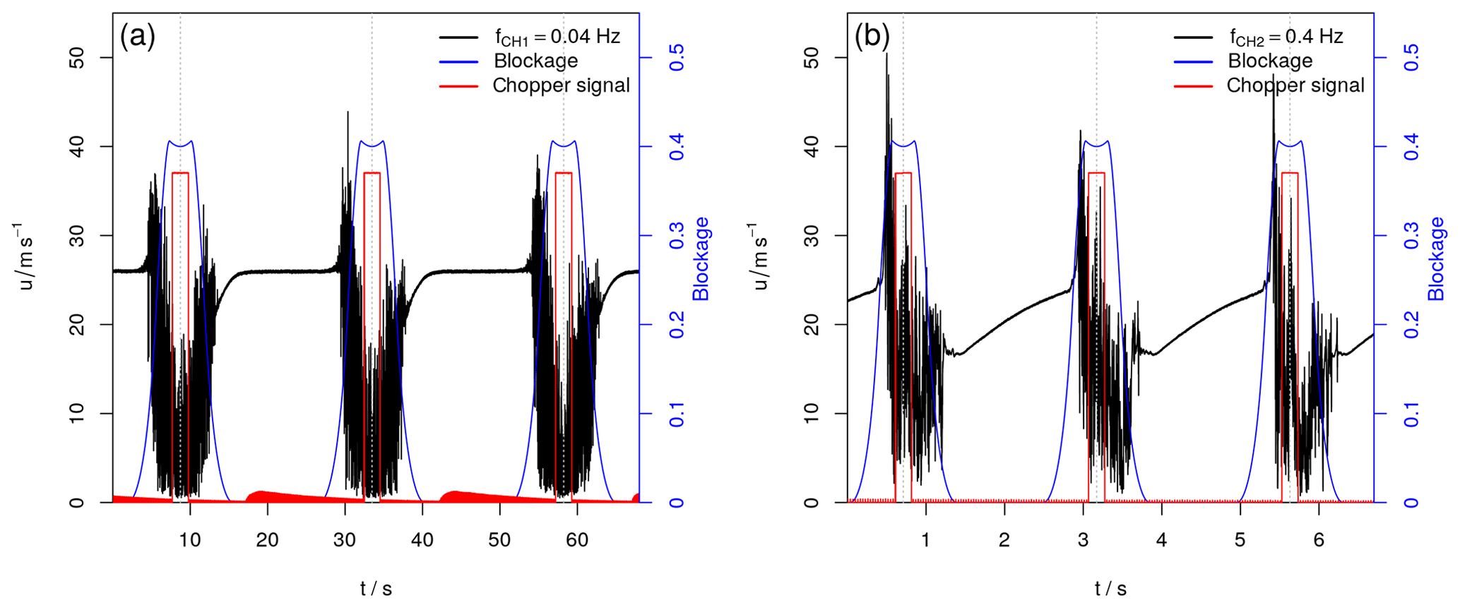
Figure 3 Gust produced by the chopper, measured at the centerline 5.425 w_CH from the chopper blade: (a) $f_{{\mathrm{CH}}_{\mathrm{1}}}=\mathrm{0.04}$ Hz, (b) $f_{{\mathrm{CH}}_{\mathrm{2}}}=\mathrm{0.4}$ Hz. The blue curve indicates the blockage, the red curve the signal from the induction sensor, and the gray dashed lines the moment when the chopper blade is horizontally aligned with the inlet.

3.1 Analysis of the time series

In Fig. 3, a part of the time series (black) that includes three inverse gusts is plotted for both chopper frequencies. In addition, the blockage induced by the chopper (blue) and the signal from the induction sensor (red) are plotted. The measurements were carried out at the centerline 5.425 w_CH from the chopper blade. Looking at Fig. 3a ($f_{{\mathrm{CH}}_{\mathrm{1}}}=\mathrm{0.04}$ Hz), it can be seen that the velocity first increases when the chopper blade enters the inlet. The velocity then decreases drastically and fast when the blockage of the inlet due to the chopper blade increases, and it recovers eventually after the chopper blade left the inlet. Between the inverse gusts, the velocity equals the inflow velocity and has a turbulence intensity of 0.3 % as in the empty test section. While the inverse gusts evolve similarly, differences in the turbulent fluctuations are present. In the case of $f_{{\mathrm{CH}}_{\mathrm{2}}}$ (see Fig. 3b) the result looks similar with the difference that the fluctuations induced by the chopper are stronger and can reach values above 50 m s⁻¹, which is twice the inflow velocity. In addition, the velocity can not recover between the inverse gusts. Instead, it increases until the chopper blade enters the inlet anew to create the next inverse gust. This indicates that the recovery time of the mean velocity to u₀ between the gusts needs to be taken into account in future experiments. One possibility to avoid the gusts interacting with each other at high chopper frequencies would be to change the duty cycle, i.e., to use a chopper blade with only one arm.

Figure 4 shows the energy spectral density E(f) plotted over the frequency f of the two above-presented time series measured at the centerline 5.425 w_CH downstream of the chopper blade. At low frequencies, the spectrum is approximately constant but superimposed with the peak of the chopper frequency and its harmonics. From f≈10 Hz, the energy spectral density decays with increasing frequency according to $E\left(f\right)\propto f^{-\mathrm{5}/\mathrm{3}}$ up to f≈1000 Hz. Kolmogorov predicted a scaling of the wave-number energy spectrum E(k) according to $k^{-\mathrm{5}/\mathrm{3}}$ for “ideal” turbulence with dissipation in equilibrium (see Kolmogorov, 1941a, b). By means of Taylor's hypothesis of frozen turbulence, the wave-number spectrum can be converted to a spectrum in the frequency domain and the scaling becomes $f^{-\mathrm{5}/\mathrm{3}}$ (e.g., Laizet et al., 2015). At first glance, it is therefore tempting to interpret the scaling found in the presented energy spectra as an indication of the existence of features of homogeneous, isotropic turbulence. However, as the measurements that are presented here are carried out in the highly turbulent near wake of the chopper blade, Kolmogorov's theory is not expected to hold. Other studies such as the one presented by Alves Portela et al. (2017) find a similar behavior of the turbulence in the near wake of a square prism. The origin of the $-\mathrm{5}/\mathrm{3}$ scaling in our measurements may therefore be the intermittency of the turbulent flow, as for example Laizet et al. (2015) and Zhou et al. (2019) discuss.

Figure 4 Energy spectral density of the measured time series at the centerline 5.425 w_CH from the inlet for the chopper frequencies (a) $f_{{\mathrm{CH}}_{\mathrm{1}}}=\mathrm{0.04}$ Hz and (b) $f_{{\mathrm{CH}}_{\mathrm{2}}}=\mathrm{0.4}$ Hz. The blue line indicates a power-law decay according to $E\left(f\right)\propto f^{-\mathrm{5}/\mathrm{3}}$.

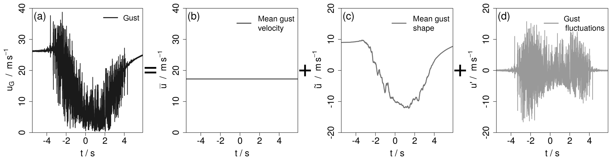
Figure 5 Example of a triple decomposition of the inverse gust $u_{\mathrm{G}}=\stackrel{\mathrm{‾}}{u}+\stackrel{\mathrm{̃}}{u}+u^{\prime }$ (a) into its mean velocity $\stackrel{\mathrm{‾}}{u}$ (b), the underlying inverse gust shape $\stackrel{\mathrm{̃}}{u}$ (c), and the fluctuations u^′ (d).

The investigation of the gust time series and the energy spectral density shows how the recurring inverse gust generated by the chopper can be decomposed into three parts: the mean velocity of the inverse gust, the underlying shape of the inverse gust as a recurring, global large-scale flow structure, and the turbulence within the gust. This triple decomposition is illustrated in Fig. 5. The inverse gust (Fig. 5a) has a mean gust velocity $\stackrel{\mathrm{‾}}{u}$ (Fig. 5b) with an underlying inverse gust shape $\stackrel{\mathrm{̃}}{u}$ (Fig. 5c) with strong turbulent fluctuations u^′ (Fig. 5d), and $u_{\mathrm{G}}=\stackrel{\mathrm{‾}}{u}+\stackrel{\mathrm{̃}}{u}+u^{\prime }$. The underlying inverse gust shape is here calculated by phase-averaging the gust events and smoothing with a moving average with a window size of 0.1 s. The fluctuations are then extracted by subtracting the underlying inverse gust shape from the respective gust. As shown in Fig. 6, the energy spectrum of the whole time series E_G(f), Fig. 6a, can analogously be split into a highly energetic, low-frequency part $\stackrel{\mathrm{̃}}{E}\left(f\right)$ from the periodically recurring underlying inverse gust shape (Fig. 6b) and a high-frequency part from the gust fluctuations E^′(f) (Fig. 6c). To calculate $\stackrel{\mathrm{̃}}{E}\left(f\right)$, the time series was sampled down to $f_{\mathrm{s}}^{\prime }=\mathrm{10}$ Hz by taking every 10 000th data point. We use this method instead of applying a filter to emphasize the two distinguishable parts the spectrum is made of, and the frequency was chosen to have a small overlap between $\stackrel{\mathrm{̃}}{E}\left(f\right)$ and E^′(f). In case of E^′(f), the spectra of u^′ of all inverse gust events within the time series are calculated, and afterwards the spectra are averaged.

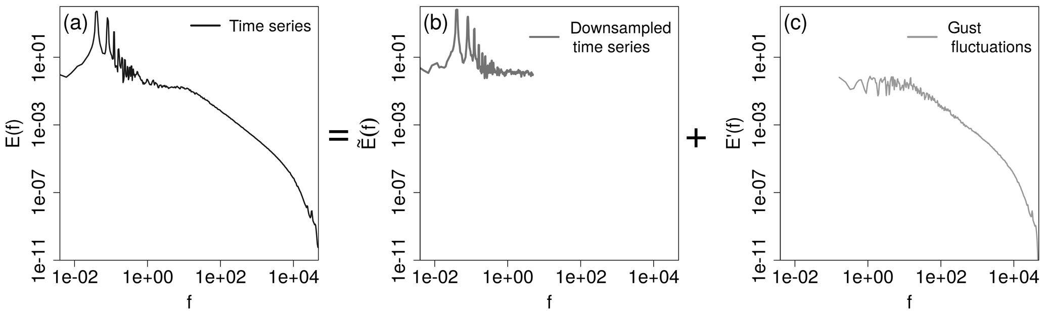
Figure 6 Example of a spectral decomposition of the inverse gust $E_{\mathrm{G}}\left(f\right)=\stackrel{\mathrm{̃}}{E}\left(f\right)+E^{\prime }\left(f\right)$ (a) into its periodic, highly energetic part $\stackrel{\mathrm{̃}}{E}\left(f\right)$ (b) and the spectrum of the fluctuations E^′(f) (c).

3.2 Mean gust flow field: $\stackrel{\mathrm{‾}}{u}$

In the following, the properties of the mean gust velocity flow field will be investigated by looking at the evolution of $\stackrel{\mathrm{‾}}{u}$ across the measured planes. The mean gust velocity is calculated by averaging the individual inverse gust events within a time series and then taking the average over all values³. The average standard deviation is determined similarly. For a better comparison between the measurements, the same window with respect to the chopper position is used for all data sets for the respective chopper frequency.

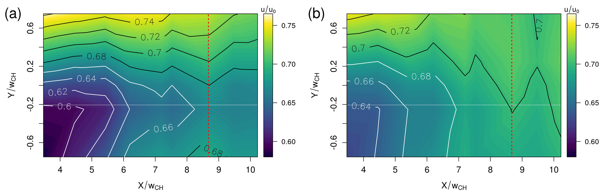
Figure 7 Interpolated surface plot of the downstream evolution of the mean velocity of the inverse gust for (a) $f_{{\mathrm{CH}}_{\mathrm{1}}}=\mathrm{0.04}$ Hz and (b) $f_{{\mathrm{CH}}_{\mathrm{2}}}=\mathrm{0.4}$ Hz. The red dashed line marks the downstream position of the YZ plane.

In Fig. 7, the downstream evolution of the average mean gust velocity that is normalized by the inflow velocity is presented as an interpolated surface plot for both chopper frequencies. For both cases, the mean gust velocity evolves similarly downstream in the test section. Close to the inlet, the flow is inhomogeneous along the span-wise direction. The lowest velocities are found at the root side of the chopper blade at $X/w_{\mathrm{CH}}=\mathrm{3.475}$ and $Y/w_{\mathrm{CH}}=-\mathrm{0.75}$. At the tip side of the chopper blade at $X/w_{\mathrm{CH}}=\mathrm{3.475}$ and $Y/w_{\mathrm{CH}}=\mathrm{0.75}$, the velocities are highest. A velocity difference of 0.14 u₀ (or 3.5 m s⁻¹) in the case of $f_{{\mathrm{CH}}_{\mathrm{1}}}=\mathrm{0.04}$ Hz and 0.08 u₀ (or 2.0 m s⁻¹) for $f_{{\mathrm{CH}}_{\mathrm{2}}}=\mathrm{0.4}$ Hz is found in the span-wise direction at $X/w_{\mathrm{CH}}=\mathrm{3.475}$. With increasing downstream position, the flow field becomes more homogeneous in the span-wise direction, and the average gust velocity reaches approximately 70 % of the inflow velocity at the end of the measurement plane. While the flow fields evolve in principle similarly, the velocities are higher and the flow field is less asymmetric in the case of the high chopper frequency.

In Fig. 8, the mean gust velocity that is normalized by the inflow velocity is plotted in the YZ plane at $X/w_{\mathrm{CH}}=\mathrm{8.675}$ in a similar manner. In the case of $f_{{\mathrm{CH}}_{\mathrm{1}}}$, the velocity is lowest in the upper left corner ($Y/w_{\mathrm{CH}}=-\mathrm{0.75}$, $Z/w_{\mathrm{CH}}=\mathrm{0.75}$) where the chopper blade enters the inlet and highest in the bottom right corner ($Y/w_{\mathrm{CH}}=\mathrm{0.75}$, $Z/w_{\mathrm{CH}}=-\mathrm{0.75}$) where the chopper blade leaves the inlet first. In the case of $f_{{\mathrm{CH}}_{\mathrm{2}}}$, the velocity is higher in the right half (Y>0) than in the left half (Y<0).

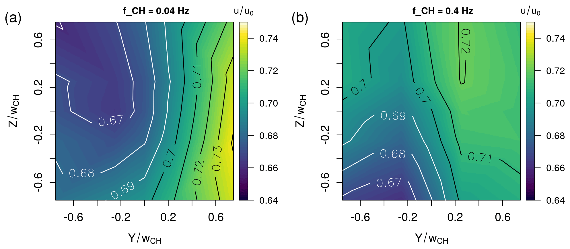
Figure 8 Interpolated surface plot of the mean velocity of the inverse gust in the YZ plane 8.675 w_CH downstream of the chopper blade for (a) $f_{{\mathrm{CH}}_{\mathrm{1}}}=\mathrm{0.04}$ Hz and (b) $f_{{\mathrm{CH}}_{\mathrm{2}}}=\mathrm{0.4}$ Hz.

Next, the average turbulence intensity of the inverse gust is plotted. For this, the average over the standard deviations σ_i of the N inverse gusts within the time series is calculated, ${\stackrel{\mathrm{‾}}{\mathit{\sigma }}}_{\mathrm{G}}=\frac{\mathrm{1}}{N}\sum _{i=\mathrm{1}}^N{\mathit{\sigma }}_i$, and divided by the average gust velocity, TI${}_{\mathrm{G}}={\stackrel{\mathrm{‾}}{\mathit{\sigma }}}_{\mathrm{G}}/\stackrel{\mathrm{‾}}{u}$. Note that this gives a global turbulence intensity that takes both the inverse gust shape and the fluctuations into account. The result is presented as an interpolated contour plot in Fig. 9. In the case of the lower chopper frequency, the highest turbulence intensities are found closest to the inlet, and the maximum turbulence intensity, TI${}_{\mathrm{G},{\max }_{\mathrm{1}}}=\mathrm{60}$ %, is measured at X=3.475 w_CH and $Y/w_{\mathrm{CH}}=-\mathrm{0.25}$. The values are very high because the global turbulence intensity is used. The local turbulence intensity is on the order of magnitude of 25 %. The flow field is asymmetric but becomes more homogeneous farther downstream when the turbulence intensity decreases. The lowest value, TI${}_{\mathrm{G},{\min }_{\mathrm{1}}}=\mathrm{34}$ %, is found at $X/w_{\mathrm{CH}}=\mathrm{10.225}$ and $Y/w_{\mathrm{CH}}=\mathrm{0.75}$. While the evolution as such looks similar in the case of the high chopper frequency, the turbulence intensities are lower, decreasing from TI${}_{\mathrm{G},{\max }_{\mathrm{2}}}=\mathrm{41}$ % at $X/w_{\mathrm{CH}}=\mathrm{4.45}$ and $Y/w_{\mathrm{CH}}=-\mathrm{0.25}$ to TI${}_{\mathrm{G},{\min }_{\mathrm{2}}}=\mathrm{24}$ % at $X/w_{\mathrm{CH}}=\mathrm{10.225}$ and $Y/w_{\mathrm{CH}}=\mathrm{0.75}$.

Figure 9 Interpolated surface plot of the turbulence intensity of the inverse gust for (a) $f_{{\mathrm{CH}}_{\mathrm{1}}}=\mathrm{0.04}$ Hz and (b) $f_{{\mathrm{CH}}_{\mathrm{2}}}=\mathrm{0.4}$ Hz. The red dashed line marks the downstream position of the YZ plane.

As presented in Fig. 10, the average gust turbulence intensity also varies spatially in the YZ plane ($X/w_{\mathrm{CH}}=\mathrm{8.675}$). In the case of $f_{{\mathrm{CH}}_{\mathrm{1}}}$ (Fig. 10a), the turbulence intensity is lowest at the vertical wind tunnel walls in the upper half of the measurement field and highest in the center in the bottom half. For the high chopper frequency, the average gust turbulence intensity is lowest in the top half of the measurement field and increases in the bottom half.

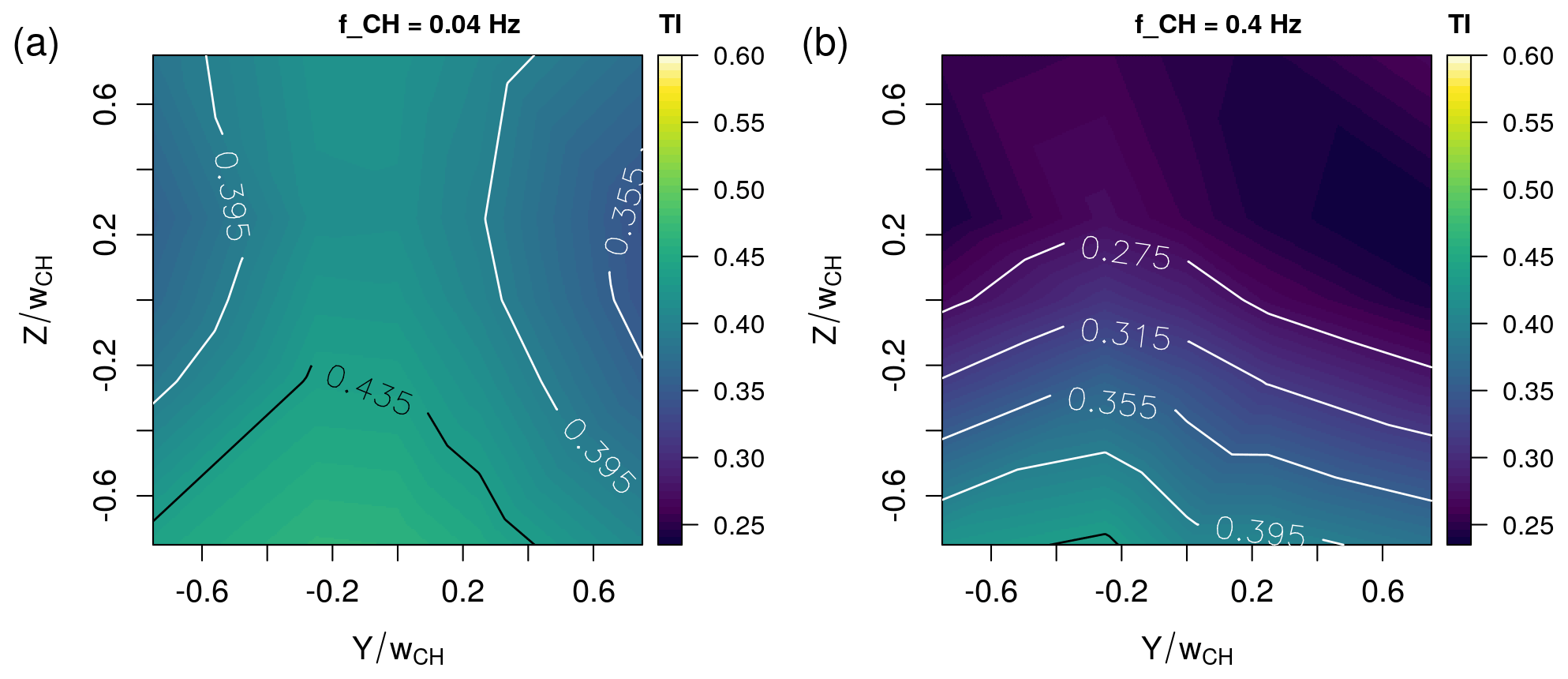
Figure 10 Interpolated surface plot of the turbulence intensity of the inverse gust in the YZ plane 8.675 w_CH downstream of the chopper blade for (a) $f_{{\mathrm{CH}}_{\mathrm{1}}}=\mathrm{0.04}$ Hz and (b) $f_{{\mathrm{CH}}_{\mathrm{2}}}=\mathrm{0.4}$ Hz.

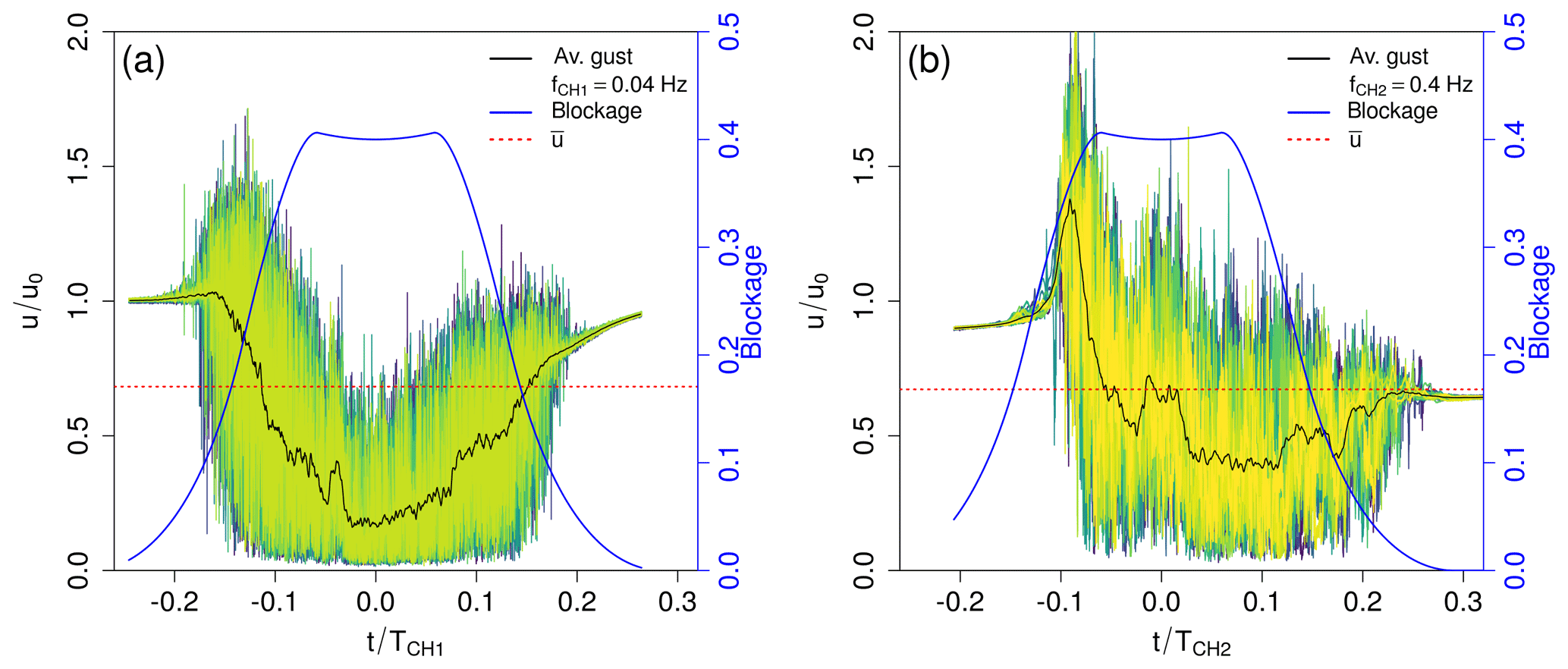
Figure 11 Plot of all inverse gusts captured in the time series measured at the centerline 5.425 w_CH downstream of the chopper blade for a chopper frequency of (a) $f_{{\mathrm{CH}}_{\mathrm{1}}}=\mathrm{0.04}$ Hz and (b) $f_{{\mathrm{CH}}_{\mathrm{2}}}=\mathrm{0.4}$ Hz. In different colors (dark blue–green–yellow color map), the inverse gust events are plotted, in black the smoothed average inverse gust is marked, and in blue the blockage is added with the corresponding axis on the right side.

3.3 Underlying inverse gust shape: $\stackrel{\mathrm{̃}}{u}$

In the following, the underlying inverse gust shape $\stackrel{\mathrm{̃}}{u}$ will be investigated. For this, only the inverse gust segments of each time series are taken into consideration. Exemplarily, in Fig. 11, all inverse gusts from the respective time series measured at the two chopper frequencies and at the centerline at X=5.425 w_CH are plotted normalized by the inflow velocity over the time t. t is normalized by the chopper period $T_{\mathrm{CH}}=\mathrm{1}/f_{\mathrm{CH}}$. Here $t/T_{\mathrm{CH}}=\mathrm{0}$ denotes the horizontal alignment of the chopper blade in the inlet. In black, the smoothed average inverse gust is plotted⁴, and in blue, the blockage of the wind tunnel is added. For both chopper frequencies, the single inverse gusts show strong fluctuations. The maximum velocity fluctuations can reach 1.8 u₀ (or u≈45 m s⁻¹) ($f_{{\mathrm{CH}}_{\mathrm{1}}}=\mathrm{0.04}$ Hz) or 2.16 u₀ (or u≈54 m s⁻¹) ($f_{{\mathrm{CH}}_{\mathrm{2}}}=\mathrm{0.4}$ Hz). While the inverse gust generated with a chopper frequency of $f_{{\mathrm{CH}}_{\mathrm{1}}}=\mathrm{0.04}$ Hz shows a smaller increase in the velocity in the beginning and is mainly characterized by a strong velocity deficit, in the case of the faster chopper frequency, $f_{{\mathrm{CH}}_{\mathrm{2}}}=\mathrm{0.4}$ Hz, the increase in the beginning is much stronger and the velocity deficit afterwards less pronounced. The strong velocity increase can be explained by the faster blockage of the inlet in the case of $f_{{\mathrm{CH}}_{\mathrm{2}}}$: as the mass flow rate is expected to be similar, the faster blockage forces the flow to adapt more quickly, which leads to a sudden acceleration. Because the flow has more time to adapt in the case of $f_{{\mathrm{CH}}_{\mathrm{1}}}$, only little to no acceleration is present. For both chopper frequencies, the highly unsteady flow induces in addition strong fluctuations, and the combination of these strong fluctuations with the acceleration of the flow in the case of $f_{{\mathrm{CH}}_{\mathrm{2}}}$ leads to those extreme velocity peaks up to 2.16 u₀. In both cases, a small velocity increase around $t/T\approx \mathrm{0.03}$ is present. Its origin may lay in a flow change occurring when the chopper blade leaves the upper corner at the inner side of the inlet: the chopper blade rotates and progressively blocks the flow at the inlet of the test section. Once the blade has fully entered the inlet, the upper part of the test section is gradually unblocked, starting at the upper inner corner. The pressurized air is then abruptly released towards the low-pressure area behind the chopper blade, which leads to a sudden increase in the velocity as the flow is entrained into the wake of the blade before the flow adapts. Similar phenomena may happen when the chopper blade leaves the inlet. As the flow has more time to adapt in the case of $f_{{\mathrm{CH}}_{\mathrm{1}}}$, the increase around $t/T\approx \mathrm{0.03}$ is less pronounced.

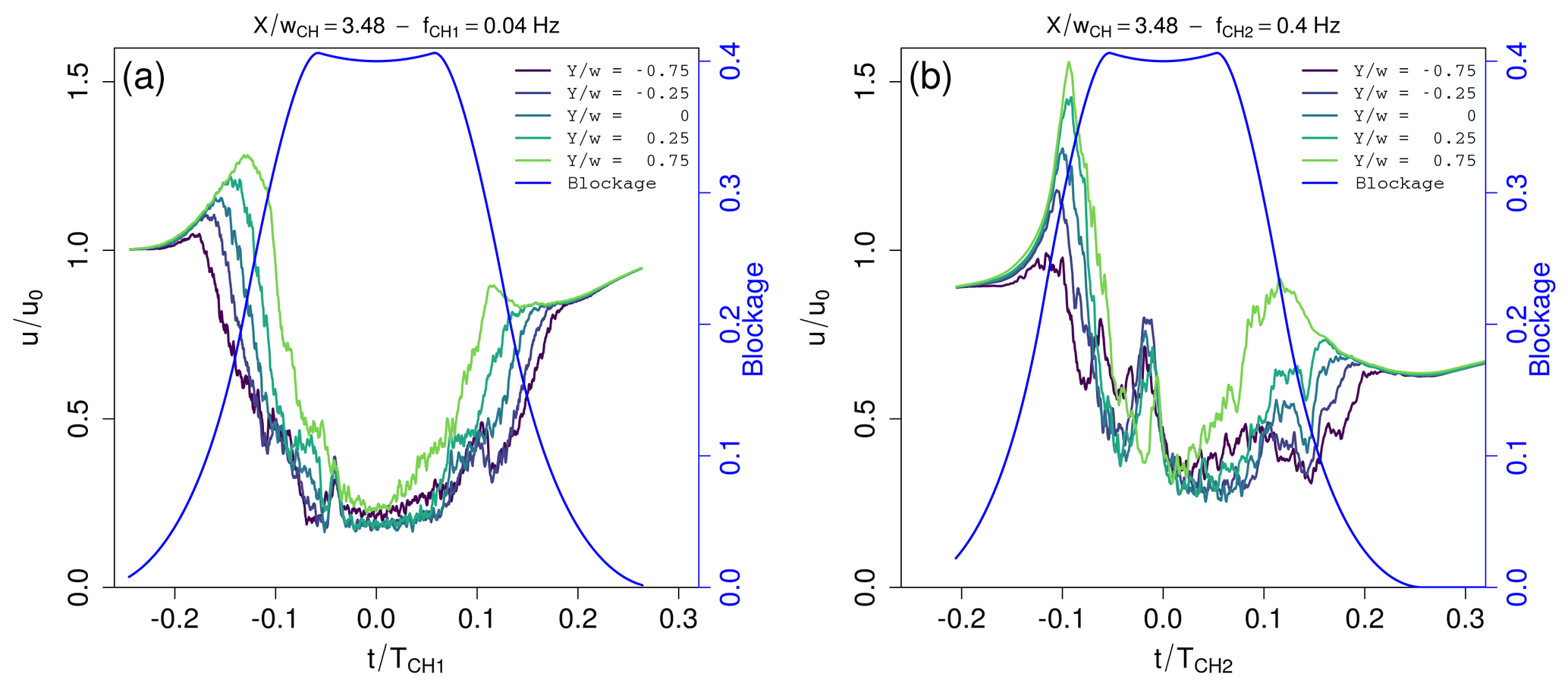
Figure 12 Span-wise evolution of the smoothened average inverse gust at $X/w_{\mathrm{CH}}=\mathrm{3.475}$ with respect to the chopper blade position. The inverse gust as measured by the respective sensor is plotted over the normalized time, where $t/T_{\mathrm{CH}}=\mathrm{0}$ indicates that the chopper blade is aligned horizontally in the inlet, and the blockage is added in blue with the blue axis on the right side. The chopper frequencies are (a) $f_{{\mathrm{CH}}_{\mathrm{1}}}=\mathrm{0.04}$ Hz and (b) $f_{{\mathrm{CH}}_{\mathrm{2}}}=\mathrm{0.4}$ Hz.

To increase the understanding of the underlying inverse gust shape $\stackrel{\mathrm{̃}}{u}$ across the width of the wind tunnel, Fig. 12 shows the smoothed average inverse gust that is normalized by the inflow velocity and plotted over t∕T_CH for all span-wise positions and both chopper frequencies at $X/w_{\mathrm{CH}}=\mathrm{3.475}$. In the case of a low chopper frequency (Fig. 12a), the inverse gust shape itself is similar for all span-wise positions. The brief increase in the velocity that exceeds the inflow velocity is followed by a rapid velocity decrease (18 m s⁻¹ in 2.5 s which is significantly stronger than the decrease of 9.8 m s⁻¹ in 2.8 s given as an example for an EOG according to the IEC-61400-1 standard). Then, there is a slight and short velocity increase around $t/T\approx \mathrm{0.03}$, and the velocity recovers once the chopper blade leaves the inlet. From $Y/w_{\mathrm{CH}}=-\mathrm{0.75}$ where the chopper blade enters the test section first with the blade root side to $Y/w_{\mathrm{CH}}=\mathrm{0.75}$ where the chopper blade enters the test section last with the blade tip side, the characteristic time of the inverse gust decreases and its amplitude increases. This is in agreement with the interpretation that a faster blockage leads to a stronger increase in the velocity at the beginning of the inverse gust. The change of the blockage is faster at the tip side of the chopper blade than at the root side due to the radially changing velocity of the chopper, and therefore, the amplitude of the inverse gust increases towards $Y/w_{\mathrm{CH}}=\mathrm{0.75}$. In addition, the local blockage is at first higher at the inner side of the test section. This combination leads to a higher, later velocity peak at the outer side of the test section. The abovementioned small, short increase in velocity around $t/T\approx \mathrm{0.03}$ is more pronounced at the measurement positions towards the inner side of the inlet. This is in agreement with the abovementioned release of the pressurized air when the chopper blade gradually unblocks the upper side of the inlet while entering.

These observations also hold for the high chopper frequency (Fig. 12b) but in a more pronounced manner.

Moving downstream to the last measurement position at $X/w_{\mathrm{CH}}=\mathrm{10.225}$ shows how the inverse gust is transported in the stream-wise direction (see Fig. 13). In the case of the low chopper frequency (Fig. 13a), the inverse gust disperses, i.e., the characteristic time increases while the amplitude decreases. The minimal velocity within the inverse gust increases while the velocity peak is not present anymore. Additionally, the small, quick velocity increase at $t/T\approx \mathrm{0.03}$ can not be distinguished anymore. Also, the underlying inverse gust shape homogenizes and evolves similarly for all span-wise positions. In comparison, the underlying inverse gust shape imprinted onto the flow with a higher chopper frequency (see Fig. 13b) preserves some variation in the span-wise direction. While the structure disperses as well, the velocity peak at the beginning of the structure is still visible. Due to the downstream transport of the inverse gust, the velocity peaks are found later with respect to the radial chopper blade position that is indicated by the blockage.

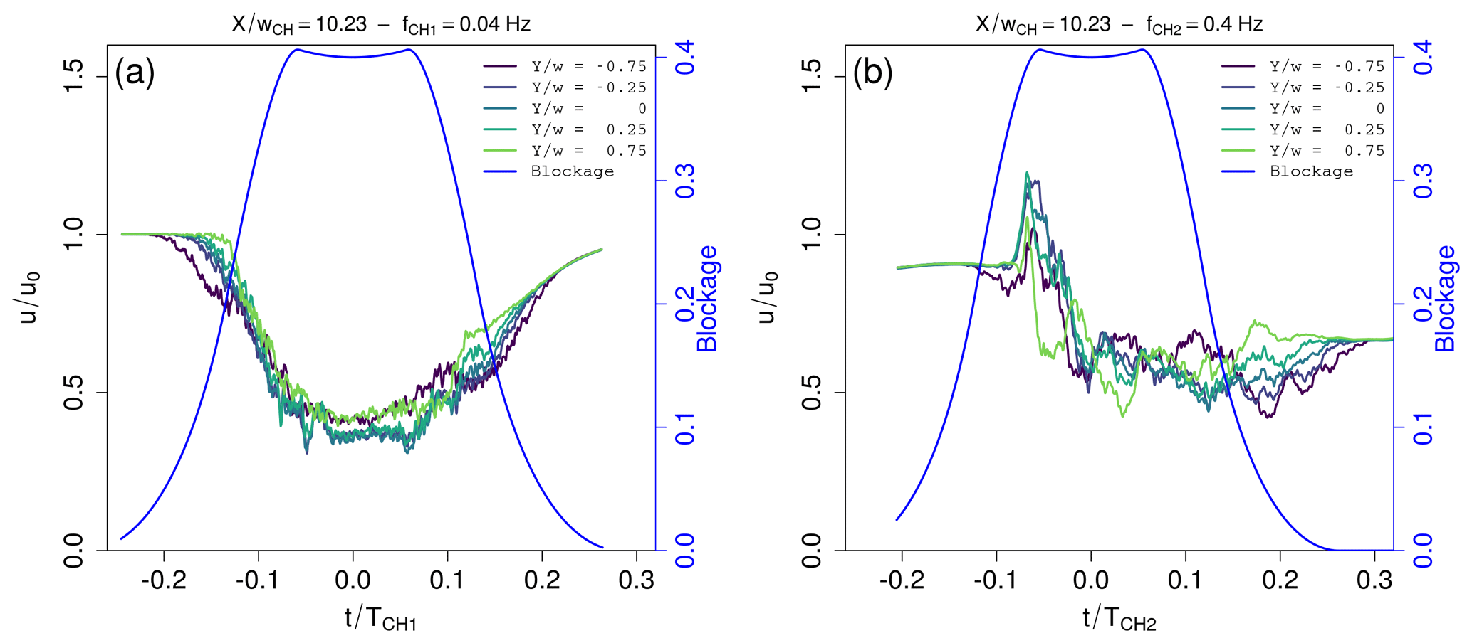
Figure 13 Span-wise evolution of the smoothed average inverse gust at $X/w_{\mathrm{CH}}=\mathrm{10.225}$ with respect to the chopper blade position. The inverse gust as measured by the respective sensor is plotted over the normalized time, where $t/T_{\mathrm{CH}}=\mathrm{0}$ indicates that the chopper blade is aligned horizontally in the inlet, and the blockage is added in blue with the blue axis on the right side. The chopper frequencies are (a) $f_{{\mathrm{CH}}_{\mathrm{1}}}=\mathrm{0.04}$ Hz and (b) $f_{{\mathrm{CH}}_{\mathrm{2}}}=\mathrm{0.4}$ Hz.

With a chopper blade width of w_CH=20 cm as presented in this setup, the inverse gust amplitude is higher than proposed by the IEC-64100-1 standard. The changes in the velocity can be rapid, for example approximately 18 m s⁻¹ in 2.5 s in the case of $f_{{\mathrm{CH}}_{\mathrm{1}}}=\mathrm{0.04}$ Hz and up to 25 m s⁻¹ in 0.25 s in the case of $f_{{\mathrm{CH}}_{\mathrm{2}}}=\mathrm{0.4}$ Hz.

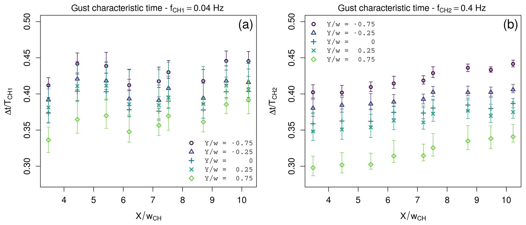
Figure 14 Average normalized characteristic time Δt∕T_CH of the gusts at the respective span-wise and downstream positions for (a) $f_{{\mathrm{CH}}_{\mathrm{1}}}=\mathrm{0.04}$ Hz and (b) $f_{{\mathrm{CH}}_{\mathrm{2}}}=\mathrm{0.4}$ Hz.

In order to quantify the characteristic time of the inverse gust and its dispersion, Fig. 14 shows the downstream evolution of the gust characteristic time Δt∕T_CH that is normalized by the chopper period for both chopper frequencies and all horizontal measurement positions. The gust characteristic time is calculated by taking the absolute value of the normalized gust fluctuations $u^{\prime }/\stackrel{\mathrm{‾}}{u}$ to find the interval in which the fluctuations frequently exceed a threshold set to be 0.025. This threshold was chosen to be low enough to capture the beginning of the gust well while also being high enough to neglect possible unexpected dynamics in the laminar part between the gust. In addition, the thresholds 0.02 and 0.03 were used to determine errors from the sensitivity of this method towards different thresholds. The results are plotted in the form of error bars that may be asymmetric. For both chopper frequencies, the gust characteristic time increases with increasing distance from the inlet as the gust disperses downstream. Additionally, the gust characteristic time is longer for the inner span-wise measurement positions $Y/w_{\mathrm{CH}}=-\mathrm{0.75}$ and $Y/w_{\mathrm{CH}}=-\mathrm{0.25}$ than for the outer span-wise positions (Y≥0), because the root side of the chopper blade passes by more slowly than the tip side. However, with respect to the errors, the gust characteristic times are similar in the case of $f_{{\mathrm{CH}}_{\mathrm{1}}}$. Quantitatively, the gust characteristic time scales anti-proportionally with the chopper frequency, which is nicely shown by the similar normalized gust characteristic times for the two chopper frequencies. The approximate gust characteristic times are $\mathrm{\Delta }t\left(f_{{\mathrm{CH}}_{\mathrm{1}}}\right)\approx \mathrm{10}$ s, and $\mathrm{\Delta }t\left(f_{{\mathrm{CH}}_{\mathrm{2}}}\right)\approx \mathrm{0.9}$ s. $\mathrm{\Delta }t\left(f_{{\mathrm{CH}}_{\mathrm{1}}}\right)\approx \mathrm{10}$ s matches the characteristic time of the IEC EOG Δt_IEC=10.5 s closely. $\mathrm{\Delta }t\left(f_{{\mathrm{CH}}_{\mathrm{2}}}\right)\approx \mathrm{0.9}$ s is scaled to wind tunnel dimensions. The ratio of chord length c and gust characteristic time should be constant, which is achieved for the airfoil that we will use with c=0.09 m.

Figure 15 Energy spectral density of all inverse gusts (blue–green–yellow color map) with the average spectrum plotted in red and a decay according to $E\left(f\right)\propto f^{-\mathrm{5}/\mathrm{3}}$ plotted in blue. The downstream position is X=5.425 w_CH, the measurement was carried out at the centerline, and the chopper frequency is (a) $f_{{\mathrm{CH}}_{\mathrm{1}}}=\mathrm{0.04}$ Hz and (b) $f_{{\mathrm{CH}}_{\mathrm{2}}}=\mathrm{0.4}$ Hz.

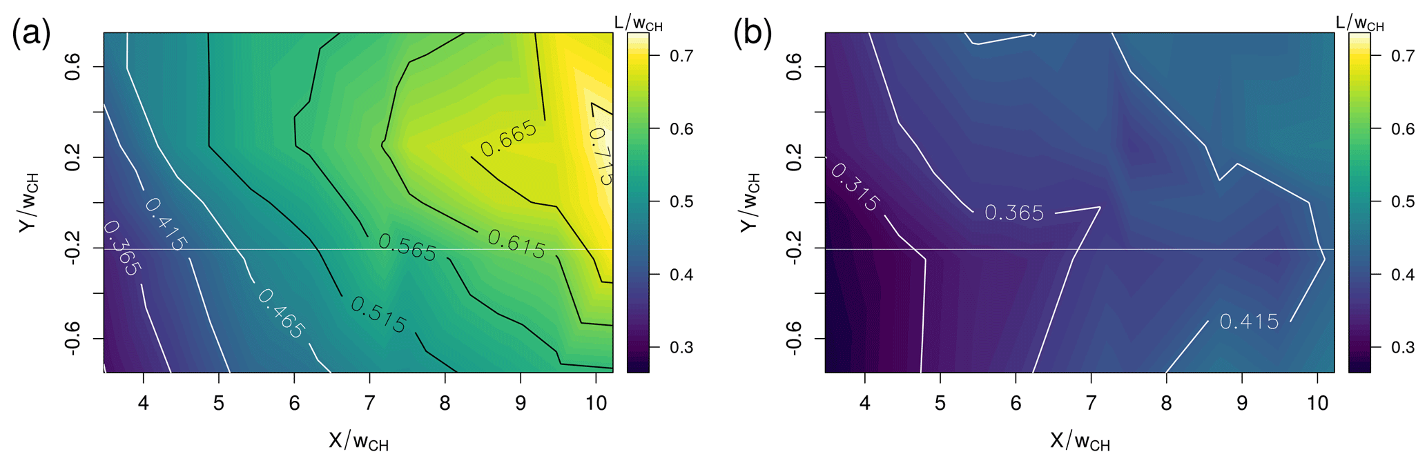
Figure 16 Interpolated surface plot of the integral length scale of the gust fluctuations for (a) $f_{{\mathrm{CH}}_{\mathrm{1}}}=\mathrm{0.04}$ Hz and (b) $f_{{\mathrm{CH}}_{\mathrm{2}}}=\mathrm{0.4}$ Hz.

3.4 Gust fluctuations: u^′

After investigating the mean gust properties and the underlying inverse gust shape, next, some turbulence characteristics of the gust will be discussed by investigating the gust fluctuations u^′. Figure 15 shows the energy spectral density of the turbulent fluctuations u^′ (see Fig. 11d) of all individual inverse gusts captured in the above-discussed time series measured at $X/w_{\mathrm{CH}}=\mathrm{5.425}$ for the respective chopper frequencies. In addition, the average over all spectra is plotted in red, and the decay according to $E\left(f\right)\propto f^{-\mathrm{5}/\mathrm{3}}$ in the inertial subrange is indicated in blue. The plots show that the turbulence within the inverse gust has approximately the same energy spectrum for all inverse gusts. The inertial subrange follows a decay according to $E\left(f\right)\propto f^{-\mathrm{5}/\mathrm{3}}$ in the frequency range between 20 Hz $\le f\le \mathrm{2000}$ Hz ($f_{{\mathrm{CH}}_{\mathrm{1}}}=\mathrm{0.04}$ Hz) and 20 Hz $\le f\le \mathrm{5000}$ Hz ($f_{{\mathrm{CH}}_{\mathrm{2}}}=\mathrm{0.4}$ Hz). As mentioned above, we do not expect Kolmogorov's theory to hold in this flow, which leads to the interpretation that the origin of the $-\mathrm{5}/\mathrm{3}$ scaling of the inertial subrange may be the intermittency of the flow (Laizet et al., 2015; Zhou et al., 2019).

To further characterize the gust turbulence, the one-dimensional energy spectrum is as suggested by Hinze (1975) used to calculate the integral length scale $L=\underset{f\to \mathrm{\infty }}{lim}\left(\frac{E\left(f\right)\cdot \stackrel{\mathrm{‾}}{u}}{\mathrm{4}{\mathit{\sigma }}^{\mathrm{2}}}\right)$ of the turbulence. The integral length scale presents here the large scales within the turbulence which supplements the gust characteristic time at a global scale. The results are shown for both chopper frequencies as interpolated contour plots in Fig. 16. While in the case of the lower chopper frequency $f_{{\mathrm{CH}}_{\mathrm{1}}}=\mathrm{0.04}$ Hz higher values of L are present, the evolution of L across the measurement plane behaves in principle similarly: L increases in both the span-wise direction from $Y/w_{\mathrm{CH}}=-\mathrm{0.75}$ to $Y/w_{\mathrm{CH}}=\mathrm{0.75}$ and downstream from $X/w_{\mathrm{CH}}=\mathrm{3.475}$ to $X/w_{\mathrm{CH}}=\mathrm{10.225}$. With respect to the average integral length $\stackrel{\mathrm{‾}}{L}$ over the whole flow field, the gradient in the span-wise direction is approximately 20 % in the case of $f_{{\mathrm{CH}}_{\mathrm{1}}}$ and between 20 % ($X/w_{\mathrm{CH}}=\mathrm{3.475}$) and 0.6 % ($X/w_{\mathrm{CH}}=\mathrm{10.225}$) in the case of $f_{{\mathrm{CH}}_{\mathrm{2}}}$. The downstream gradients are 63 % and 40 %, which indicates that the change in the stream-wise direction is more significant. The smallest values are found at $X/w_{\mathrm{CH}}=\mathrm{3.475}$ and $Y/w_{\mathrm{CH}}=-\mathrm{0.75}$ with L=0.25 w_CH in the case of $f_{{\mathrm{CH}}_{\mathrm{1}}}=\mathrm{0.04}$ Hz and L=0.245 w_CH in the case of $f_{{\mathrm{CH}}_{\mathrm{2}}}=\mathrm{0.4}$ Hz. As the turbulence evolves downstream, L increases and the highest values are found at the opposite corner of the flow field at $X/w_{\mathrm{CH}}=\mathrm{10.225}$ and $Y/w_{\mathrm{CH}}=\mathrm{0.25}$ with L=0.73 w_CH in the case of $f_{{\mathrm{CH}}_{\mathrm{1}}}=\mathrm{0.04}$ Hz and L=0.46 w_CH in the case of $f_{{\mathrm{CH}}_{\mathrm{2}}}=\mathrm{0.4}$ Hz.

The integral length scale is of interest when carrying out aerodynamic experiments because the interaction between the airfoil and the flow structures depends on the ratio L∕c. It is for example indicated in Cao et al. (2011) that a smaller integral length in the flow delays stall.

4 Conclusions and outlook

The chopper, a new system for the generation of strong, sudden inverse gusts in a wind tunnel, has been presented together with a first investigation of the flow generated by it. The experimental campaign was performed at 65 measurement points in the three-dimensional volume of the test section to characterize the stream-wise flow behind this new perturbation system. The focus of this study was on the identification of governing parameters that influence the unsteady flow to refine experiments in the future. The inverse gust structure induced by the chopper has been examined for a fixed inflow velocity and two different chopper frequencies, and the parameters were chosen to match the specifications of future experiments. First, the periodic flow variation that is generated each time the chopper blade crosses the inlet was discussed by means of the time series and its energy spectrum. To gain a better understanding of the inverse gust structure itself, in the next step, the gust events were brought into focus. It was shown how the inverse gust has an underlying shape with superimposed fluctuations, so that each inverse gust can be decomposed into a mean gust velocity $\stackrel{\mathrm{‾}}{u}$, the global underlying inverse gust shape $\stackrel{\mathrm{̃}}{u}$, and the high-frequency fluctuations u^′. Analogously, the decomposition can be carried out in the spectral domain. For further analysis, this triple decomposition was used to discuss the evolution of the underlying inverse gust shape that disperses downstream while the average gust velocity simultaneously increases and the global turbulence intensity decreases. The average flow field is asymmetric close to the chopper blade but becomes more homogeneous farther downstream. Some aspects of the underlying inverse gust shape were related to the physical behavior of the system, and it was explained that some mechanisms responsible for the inverse gust generation appear to be universal with respect to the chopper frequency. The gust characteristic time is anti-proportional to the chopper frequency, and the two investigated chopper frequencies generate inverse gusts with characteristic times similar to Δt_IEC and downscaled to wind tunnel dimensions where a constant ratio of airfoil chord length to gust characteristic time is aimed for. The mean gust amplitude is larger than the one proposed in the IEC-64100-1 standard for all measurements. In addition, the velocity can change rapidly. The velocity fluctuations were analyzed by means of the energy spectrum that shows a turbulence decay with an inertial subrange that decays according to $E\left(f\right)\propto f^{-\mathrm{5}/\mathrm{3}}$. The integral length scale increases downstream as the turbulence evolves, and it is of the order of magnitude of half the chopper blade width. The inverse gust can therefore be characterized by a global scale, namely its characteristic time, and an outer turbulence scale, namely the integral length.

Overall, a new system was presented that is capable of generating large, rapid velocity fluctuations while also inducing turbulence. By means of the downstream position and the chopper frequency, experiments can be carried out in different regions of the flow field that have different characteristics and different complexity. The complexity of the flow increases towards the inlet. For example, the aerodynamic behavior of an airfoil can be studied downstream where the flow is already quite homogeneous, and then it can be compared to the aerodynamic behavior of the airfoil positioned farther upstream in the inhomogeneous region where three-dimensional effects will be present. This gives an opportunity to study the effect of radial inflow changes which may cause similar effects as rotational augmentation that is observed in rotational blades due to an additional radial flow (see Bangga, 2018).

This investigation has shown us limits and opportunities of the setup and the measurements, which helps us to improve the setup in the future. The currently very high blockage induced by the chopper blade will be reduced in the future by reducing the chopper blade width. We expect this to also decrease the currently very high velocity amplitudes of the gust. Moreover, new chopper blade designs are possible that reduce the inhomogeneity of the flow field. To generate “normal” instead of inverse gusts, the design of a rotating disc with varying blockage is also possible. As the flow between the gusts has a low turbulence intensity, in addition, background turbulence can be added by installing a grid upstream of the chopper blade. To verify to what extent the gust generation mechanisms are universal with respect to the chopper frequency, more chopper frequencies need to be investigated. The experimental campaign that was presented gives a good overview of the flow evolution in the test section, but it should be complemented by measurements of all flow components and with higher spatial resolution of the measurement points. To form a comprehensive picture both in space and in time, future investigations may involve phase-averaged and/or time-resolved particle image velocimetry as well as simulations.