Real-time optimization of wind farms using modifier adaptation and machine learning

Coordinated wind farm control takes the interaction between turbines into account and improves the performance of the overall wind farm. Accurate surrogate models are the key to model-based wind farm control. In this article a modifier adaptation approach is proposed to improve surrogate models. The approach exploits plant measurements to estimate and correct the mismatch between the surrogate model and the actual plant. Gaussian process regression, which is a probabilistic nonparametric modeling technique, is used in the identification of the plant–model mismatch. The efficacy of the approach is illustrated in several numerical case studies. Moreover, challenges in applying the approach to a real wind farm with a truly dynamic environment are discussed.

1 Introduction

Currently wind turbines in a wind farm are operated to maximize their power production and minimize the loads on their structure and power electronics. The impact on the downstream turbines due to wake interactions is ignored. Such a control strategy is called greedy since it only focuses on the operation of an individual wind turbine. It is expected that a wind farm control strategy that takes the interaction between turbines into account can improve the overall performance of the wind farm (Steinbuch et al., 1988; Johnson and Thomas, 2009; Barthelmie et al., 2009).

The two main wind farm control strategies are axial induction control and wake steering (Kheirabadi and Nagamune, 2019). The idea behind axial induction control is for the blade pitch and generator torque of the upwind turbine to deviate from the greedy control settings. As a consequence, the velocity deficit in the wake behind the turbine decreases. The target net effect is an overall increase in the power production and possibly a decrease in fatigue loads. However, evaluating wind tunnel experiments (Campagnolo et al., 2016; Bartl and Sætran, 2016), high-fidelity simulations (Annoni et al., 2016) and field tests (van der Hoek et al., 2019), it is suggested that axial induction control using steady-state surrogate models to calculate the optimal control settings may be unable to improve the power production of a wind farm.

Currently the more promising wind farm control strategy using steady-state surrogate models is wake steering. The goal of wake steering is to deflect the wake away from the downwind turbine by using the yaw settings of the upwind turbine (Kheirabadi and Nagamune, 2019). Field experiments showing encouraging results were conducted by Fleming et al. (2017, 2019) and Howland et al. (2019). In these experiments lookup tables with optimal yaw settings depending on the wind conditions were created using steady-state models. The lookup tables were not updated using plant measurements. Therefore, these approaches can be seen as open-loop.

The steady-state surrogate models must be not only simple to allow optimization but also accurate to permit good performance of the model-based controller. The development of surrogate models is an active research field. One of the most popular wake models is the Jensen Park model (Jensen, 1983; Katic et al., 1987). Jiménez et al. (2010) developed one of the first steady-state wake models that described wake deflection due to yaw. A recent wake model, which is also used in this study, was presented by Bastankhah and Porté-Agel (2016). It is based on mass and momentum conservation and assumes a Gaussian distribution of the velocity deficit in the wake. Other extensions to the Jensen Park model were presented by Park and Law (2015), who assumed an inverted Gaussian function of the wake profile; Tian et al. (2015), who used a cosine shape function; and Ge et al. (2019), who analytically derived a Gaussian-shape velocity profile. The steady-state wake models are able to describe the general behavior of the wake (Barthelmie et al., 2013; Annoni et al., 2014). Nevertheless, they are just vague approximations of a complex phenomenon that is, in fact, not well understood (Veers et al., 2019).

Model-free methods using extremum-seeking (Johnson and Fritsch, 2012; Ciri et al., 2017) or game-theoretic methods (Marden et al., 2013; Gebraad et al., 2013) have been proposed to circumvent possible error-prone models in the control of wind farms. However, these methods suffer from slow convergence. Park et al. (2016, 2017) suggested using a Bayesian ascent (BA) algorithm fitting a Gaussian process (GP) regression to input–output data of the plant. A new data-driven surrogate model was created. In Doekemeijer et al. (2019a) the upstream wind velocity and turbulence intensity in the FLORIS model are first estimated from the data. The improved FLORIS model is then used in Bayesian optimization to find a GP surrogate model and optimal yaw angles of the turbines in the wind farm. Another data-driven surrogate model, using polynomial chaos expansion, was presented by Hulsman et al. (2020). Estimating the model parameters of the surrogate model to improve closed-loop control was proposed by Doekemeijer et al. (2019b). However, if the parametric model is structurally incorrect, parameter estimation is not able to remove the mismatch between surrogate model and the plant. An example in which an improved parameterization of a surrogate model was not able to remove the mismatch between a low-order model and a high-fidelity model is given in Fleming et al. (2018). Therefore, a two-step approach iteratively optimizing the plant and updating the model parameter of the surrogate model as plant measurements become available was not pursued here.

Instead, in this article a modifier adaptation (MA) approach (Marchetti et al., 2016) to wind farm control is proposed. The plant–model mismatch is identified by exploiting plant measurements, and the surrogate model is improved. In the identification of the plant–model mismatch GP regression is used. GP is a probabilistic, nonparametric modeling technique well known in the machine learning community (Rasmussen and Williams, 2006). The advantage of using GP regression in MA is that it is not bounded by specific model structures as in, e.g., parametric models. Consequently, the MA–GP approach is able to correct the surrogate model in a flexible manner (de Avila Ferreira et al., 2018) and improve the performance of the wind farm controller.

The article is structured as follows: in Sect. 2 the optimization problem is formulated. In Sect. 3 the modifier adaptation using Gaussian process regression is presented and the numerical turbine and wake models are introduced. The approach is tested numerically in Sect. 4. Section 5 discusses the application of the MA–GP approach to real wind farms. The article ends with a conclusion.

2 Problem formulation

Model-based wind farm optimization usually employs a steady-state surrogate model. Consequently, a plant–model mismatch exists, which can degrade the performance of a controller. In this article, we study the optimization problem of optimizing the power production, noting that the approach in general can handle different objective functions. The optimization problem can be formulated where $\mathbf{u}\in {\mathbb{R}}^{n_u}$ denotes the plant input variables, which are the axial induction factors and yaw angles of each turbine; $P_{\mathrm{p}}:{\mathbb{R}}^{n_u}\times {\mathbb{R}}^{n_y}\to \mathbb{R}$ is the power production to be maximized; and $\mathcal{U}\subseteq {\mathbb{R}}^{n_u}$ is the control domain, e.g., box constraints on the control inputs.

The challenge of optimizing the power production of a wind farm is that only an approximate surrogate model of the plant is available. Consequently, it is not guaranteed that the optimal point of the surrogate model coincides with the optimal point of the plant. MA treats this challenge by directly adapting the optimization problem using plant measurement to allow convergence to the overall plant optimum (Marchetti et al., 2009). The standard MA adds first-order modifiers to correct the gradient of the surrogate model. However, the estimation of the plant gradients in each iteration is experimentally expensive and the main bottleneck of the MA implementation in practice (Marchetti et al., 2016). In this article, GPs are used instead to correct the surrogate model (de Avila Ferreira et al., 2018) and, by this, alleviate the limitation of MA. The next section gives a brief introduction to GPs, before the new optimization problem of the MA–GP approach is stated.

3 Methodology

In this section the modifier adaptation approach with Gaussian processes for wind farm control is introduced in Sect. 3.1 and 3.2. Thereafter, in Sect. 3.3, the turbine and wake models used in the case study are explained.

3.1 Gaussian processes

In this section we give a brief outline of GP regression; for more information consult Rasmussen and Williams (2006). GP regression identifies an unknown function $f:{\mathbb{R}}^{n_u}\to \mathbb{R}$ from data. It is assumed that the noisy observations of f(⋅) are given by

$$\begin{array}{}\text{(1)}& y_k=f\left({\mathbf{u}}_k\right)+{\mathit{\nu }}_k,\end{array}$$

where the value f(⋅) is perturbed by Gaussian noise ν_k with zero mean and variance ${\mathit{\sigma }}_{\mathit{\nu }}^{\mathrm{2}}$, ν_k∼𝒩(0, ${\mathit{\sigma }}_{\mathit{\nu }}^{\mathrm{2}})$.

In GP regression, f(⋅) is considered a distribution over functions. In this paper, we assume this distribution has a zero mean function and the squared-exponential (SE) covariance function. The choice of the mean and covariance functions assumes a certain smoothness and continuity properties of the underlying function (Snelson and Ghahramani, 2006), which seems to be a good fit for the plant–model mismatch of the surrogate model. The SE covariance function can be expressed as follows:

$$\begin{array}{}\text{(2)}& k\left({\mathbf{u}}_i,{\mathbf{u}}_j\right)={\mathit{\sigma }}_f^{\mathrm{2}}\exp \left(-{\displaystyle \frac{\mathrm{1}}{\mathrm{2}}}{\left({\mathbf{u}}_i-{\mathbf{u}}_j\right)}^T{\mathbf{\Lambda }}^{-\mathrm{1}}\left({\mathbf{u}}_i-{\mathbf{u}}_j\right)\right),\end{array}$$

where ${\mathit{\sigma }}_f^{\mathrm{2}}$ is the covariance magnitude and $\mathbf{\Lambda }=\mathrm{diag}({\mathit{\lambda }}_{\mathrm{1}}^{\mathrm{2}}$, …, ${\mathit{\lambda }}_{n_u}^{\mathrm{2}})$ is a scaling matrix.

Due to the GP assumption the predictive distribution of f(u) at an arbitrary input u given the training data set 𝒟={U, Y} has a closed-form solution. The resulting mean μ_GP(u; 𝒟, $\widehat{\mathit{\psi }})$ can be seen as the GP prediction at u and the variance ${\mathit{\sigma }}_{\mathrm{GP}}^{\mathrm{2}}(\mathbf{u}$; 𝒟, $\widehat{\mathit{\psi }})$ as a corresponding measure of uncertainty to this prediction.

The performance of the GP is dependent on hyperparameters $\widehat{\mathit{\psi }}$. They are commonly unknown and hence need to be inferred from data. In this article the maximum likelihood estimate is used to calculate the hyperparameters. Finally, we note that the training data are explicitly required to construct the predictive distribution. For this a matrix of size M×M must be inverted, where M is the number of measurements. Clearly, this makes large data sets challenging.

3.2 Modifier adaptation with Gaussian processes

In the MA–GP approach the limitations of standard MA are overcome by replacing the modifiers with GPs (de Avila Ferreira et al., 2018). As a result, estimating the plant gradients (modifiers) in each iteration is avoided, at the cost of instead updating the GP. The optimization problem of the MA–GP approach becomes

$$\begin{array}{}\text{(3)}& {\widehat{\mathbf{u}}}_{k+\mathrm{1}}^{*}={\mathrm{argmax}}_{\mathbf{u}}P\left(\mathbf{u}\right)+{\mathit{\mu }}_{\mathrm{GP},k}\left(\mathbf{u};{\mathcal{D}}_k,{\widehat{\mathit{\psi }}}_k\right),s.t.\mathbf{u}\in \mathcal{U},\end{array}$$

where the plant–model mismatch of the cost function is modeled by μ_GP. The training set 𝒟 of the GP comprises the control inputs of the wind farm and the difference in the power production between surrogate model and plant measurements.

The MA–GP approach for wind farm optimization is visualized in Fig. 1. The power output of the surrogate model is subtracted from the noisy power measurements of the plant. The difference in power production and the control inputs creates the data set, which is used in the GP training to estimate the hyperparameters. A initial training set is required before initializing the MA–GP approach. In the plant optimization the surrogate model is corrected by the GP regression model, which uses the current data set and hyperparameters. The new optimal control input is applied to the wind farm. The MA–GP approach is a closed-loop control approach to wind farm optimization.

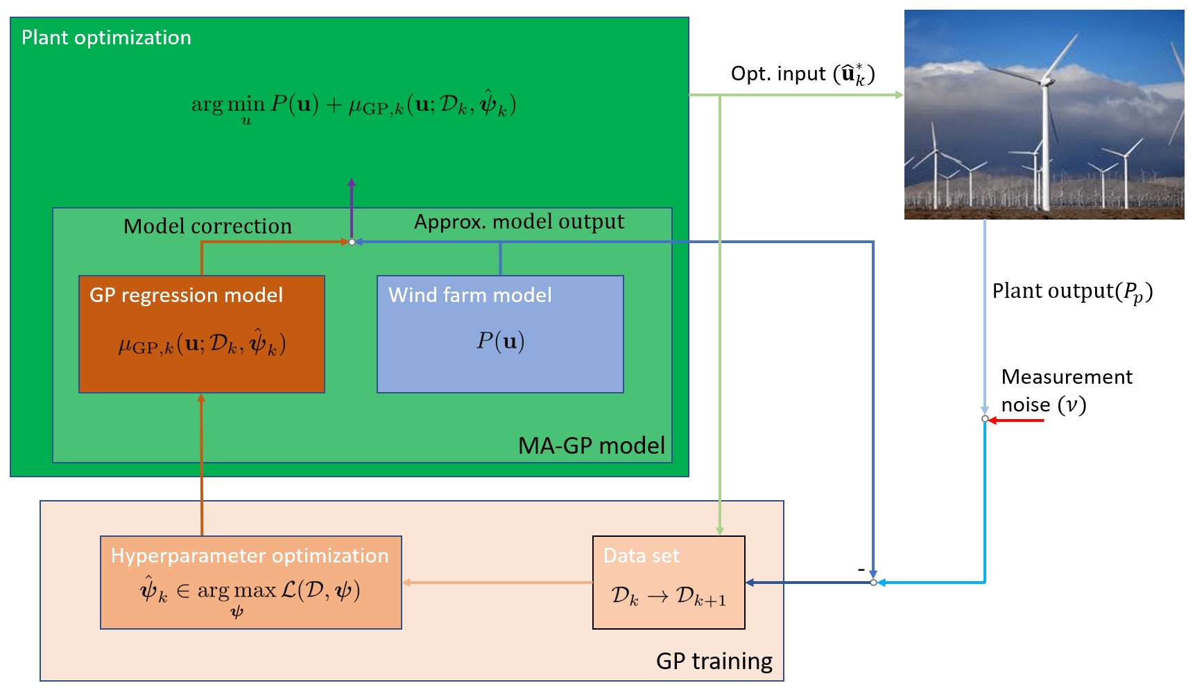
Figure 1 The basic idea of the MA–GP scheme for a wind farm. The GP regression model creates an input–output map of the control inputs to the plant–model mismatch. In the MA–GP model the GP regression model is used to correct the output of the approximate model. This MA–GP model is used in the optimization to compute optimal control inputs for the wind farm. The inputs and the difference between the measured and estimated output of plant and model, respectively, are used to update the data set 𝒟 and the hyperparameter ψ. The measured outputs of the plant are corrupted by noise. The photo of a wind farm is by Erik Wilde from Berkeley, CA, USA, https://www.flickr.com/photos/dret/24110028330/ (last access: 9 July 2020), Wind turbines in southern California 2016, https://creativecommons.org/licenses/by-sa/2.0/legalcode (last access: 9 July 2020).

In Algorithm 1 two additional steps are included in the MA–GP scheme:

• The new optimal control input is filtered with

  $$\begin{array}{}\text{(4)}& \begin{array}{rl}& {\mathbf{u}}_{k+\mathrm{1}}={\mathbf{u}}_k+\mathbf{L}\left({\widehat{\mathbf{u}}}_{k+\mathrm{1}}-{\mathbf{u}}_k\right),\\ & \mathbf{L}=\mathrm{diag}\left(l_{\mathrm{1}},\mathrm{\dots },l_{n_u}\right),l_i\in (\mathrm{0},\mathrm{1}].\end{array}\end{array}$$

  In the basic MA approach filtering the control input prevents excessive corrections. In the MA–GP approach it permits exploration around the optimal point.

• The hyperparameters are only updated when HypOpt is true, which is a user-defined condition. The hyperparameter update is usually the computational bottleneck of the MA–GP algorithm. We observed that especially for large data sets the hyperparameters do not change much from one iteration to the next. Therefore, the hyperparameters can be updated less frequently to decrease computational delay. However, it is recommend to update the hyperparameters as often as possible.

In the next subsection the turbine and wake models used in the case study are presented.

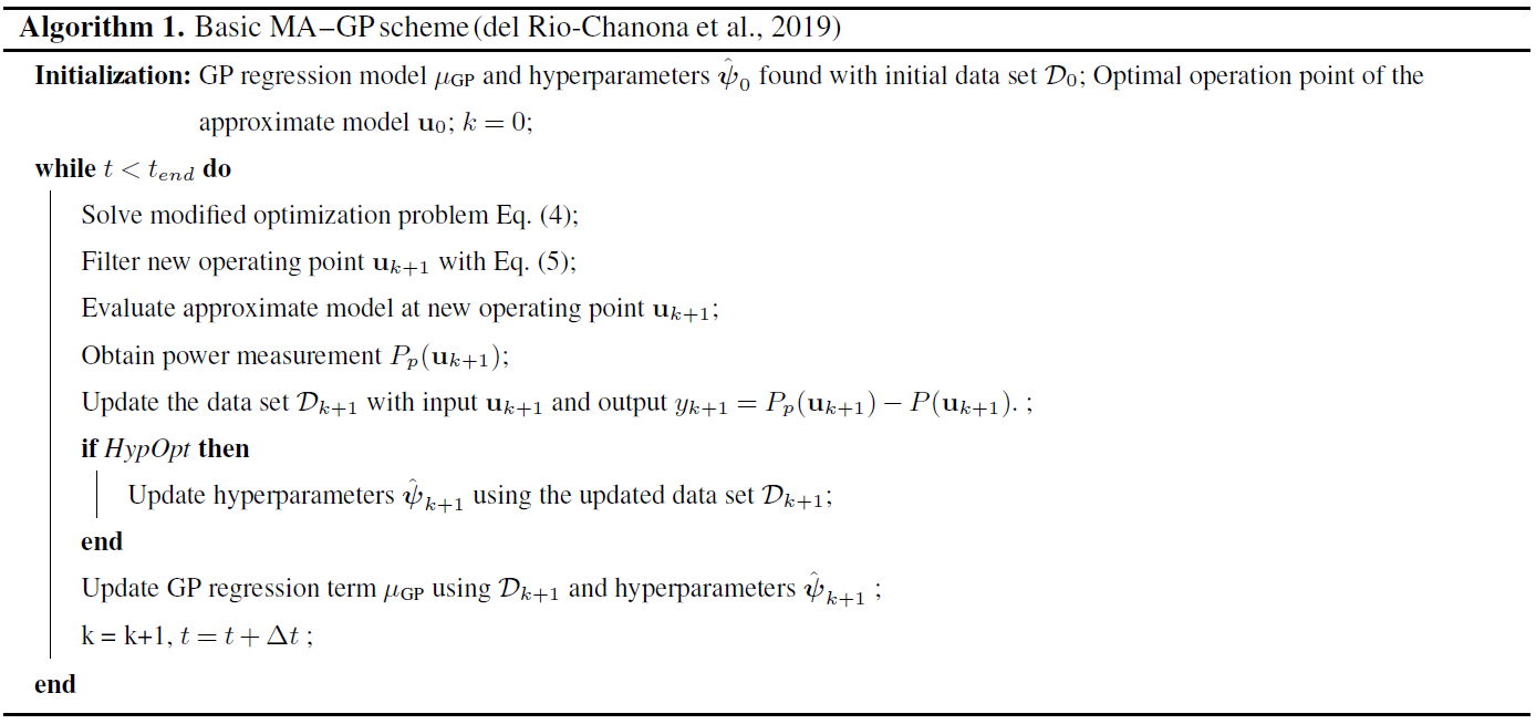
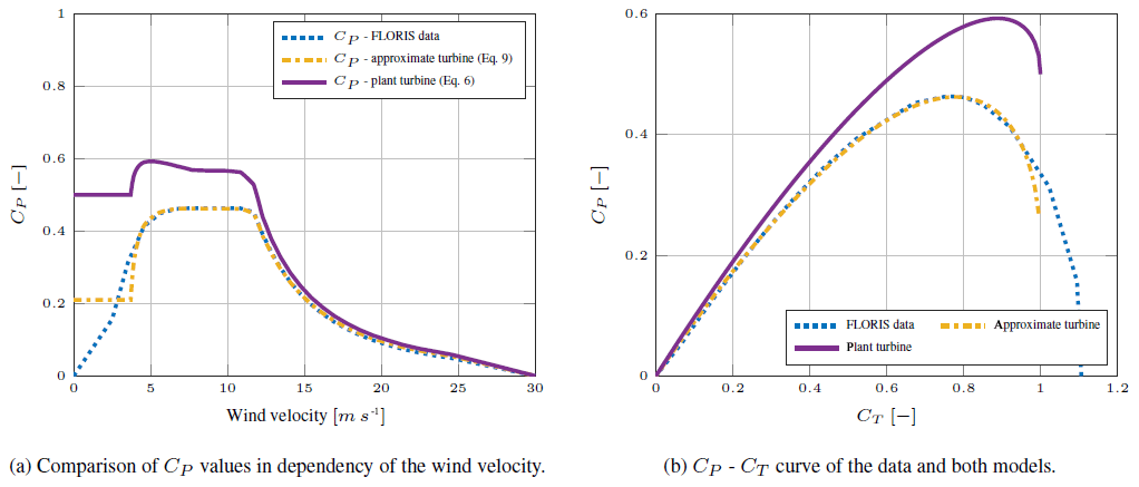
Figure 2 Comparison between data, the plant turbine and the approximate turbine model. The models give different connections between thrust and power coefficients.

3.3 Numerical turbine and wake models

Turbine and wake models are necessary for creating a model of a wind farm. The wind turbines are represented using the actuator disk theory, which couples the power and thrust coefficient, C_P and C_T (Burton et al., 2011):

$$\begin{array}{}\text{(5)}& {\displaystyle }& {\displaystyle }{C}_{\mathrm{P}}=\mathrm{4}a(\mathrm{1}-a{)}^{\mathrm{2}},\text{(6)}& {\displaystyle }& {\displaystyle }{C}_{\mathrm{T}}=\mathrm{4}a(\mathrm{1}-a),\end{array}$$

where a is the axial induction factor. The axial induction factor indicates the ratio of wind velocity reduction at the turbine disk compared to the upstream wind velocity. The steady-state power of each turbine under yaw misalignment is given by (Gebraad et al., 2016)

$$\begin{array}{}\text{(7)}& P={\displaystyle \frac{\mathrm{1}}{\mathrm{2}}}\mathit{\rho }A{C}_{\mathrm{P}}\cos {\mathit{\gamma }}^p{v}^{\mathrm{3}},\end{array}$$

where A is the rotor area, ρ the air density, p a correction factor and v the wind velocity. In actuator disk theory p=3 (Burton et al., 2011). However, based on large-eddy simulations, the turbine power yaw misalignment has been shown to match the output when p=1.88 for the NREL 5 MW turbine (Annoni et al., 2018), which we will use in this article. In the numerical study it will be important to implement both a “plant” and a model, which are different from each other. The actuator disk model will be referred to as the plant turbine model. A second adjusted actuator disk turbine model is created, which will be referred to as the approximate turbine model. The FLORIS toolbox (NREL, 2019) contains a table with wind velocities and corresponding thrust and power coefficients of the NREL 5 MW turbine. These data are fitted to create the approximate turbine model. The equation for the thrust coefficient C_T is given by Eq. (6), while for the power coefficient C_P three new parameters are identified resulting in

$$\begin{array}{}\text{(8)}& C_{\mathrm{P}}=\mathrm{7.037}a(\mathrm{0.625}-a{)}^{\mathrm{1.364}}.\end{array}$$

The approximate turbine model fit is visualized in Fig. 2. Important in the numerical example is the different connection between thrust and power coefficients of the plant and approximate turbine model (Fig. 2b). For the turbine dimensions the NREL 5 MW wind turbine is used (Jonkman et al., 2009). Consequently, the rotor diameter is D=126.4 m and the hub height H_H=90 m.

The Gaussian wake model by Bastankhah and Porté-Agel (2014, 2016) is used to model the flow in the wind farm. The three-dimensional steady-state far-wake velocity deficit is Gaussian distributed and can be estimated by

$$\begin{array}{}\text{(9a)}& {\displaystyle }& {\displaystyle \frac{\stackrel{\mathrm{‾}}{v}(x,y,z)}{{\stackrel{\mathrm{‾}}{v}}_{\mathrm{\infty }}}}=\mathrm{1}-C{e}^{-\mathrm{0.5}{\left((y-\mathit{\delta })/{\mathit{\sigma }}_y\right)}^{\mathrm{2}}}{e}^{-\mathrm{0.5}{\left(\left(z-z_{\mathrm{h}}\right)/{\mathit{\sigma }}_z\right)}^{\mathrm{2}}},\text{(9b)}& {\displaystyle }& {\displaystyle }C=\mathrm{1}-\sqrt{\mathrm{1}-{\displaystyle \frac{C_{\mathrm{T}}\cos \mathit{\gamma }}{\mathrm{8}\left({\mathit{\sigma }}_y{\mathit{\sigma }}_z/d^{\mathrm{2}}\right)}}},\end{array}$$

where z_h is the tower height, δ is the wake deflection, and σ_y and σ_z are the wake widths in lateral and vertical directions. An important variable for the model is the skew angle of the flow past a yawed turbine. The flow skew angle is approximated by

$$\begin{array}{}\text{(10)}& \mathit{\theta }\approx {\displaystyle \frac{{\mathit{\alpha }}_{\mathrm{1}}\mathit{\gamma }}{\cos \mathit{\gamma }}}\left(\mathrm{1}-\sqrt{\mathrm{1}-C_{\mathrm{T}}\cos \mathit{\gamma }}\right),\end{array}$$

where α₁ is a parameter. Bastankhah and Porté-Agel (2016) use α₁=0.3 and NREL (2019) uses α₁=0.6 to better fit high-fidelity observations. We will use the Gaussian wake model with α₁=0.3 as the approximate wake model and with α₁=0.6 as the plant wake model.

In the next section the case study using the MA–GP approach and the turbine and wake models presented here are discussed.

4 Numerical case study

In this section numerical results of the MA–GP approach are presented. The control inputs of the wind farms are the yaw angles γ_i and the thrust coefficients C_T,i of each turbine. Hence, the wind farm has 2N control inputs, where N is the number of wind turbines. The objective of the optimization is to maximize the power production $P_{\mathrm{tot}}=\sum _i{P}_i$ of the wind farm. The relative error in the power production is given by

$$\begin{array}{}\text{(11)}& \mathrm{\Theta }=\mathrm{100}{\displaystyle \frac{P_{\mathrm{p}}^{*}-{\widehat{P}}_{\mathrm{p}}}{P_{\mathrm{p}}^{*}}},\end{array}$$

where $P_{\mathrm{p}}^{*}$ is the optimal power production of the plant and ${\widehat{P}}_{\mathrm{p}}$ is the power production achieved by the MA–GP approach. The control inputs are constrained by box constraints with

$$\begin{array}{}\text{(12)}& \mathrm{0}\le C_{\mathrm{T},i}\le \mathrm{0.95},\mathrm{and}\mathrm{0}{}^{\circ }\le {\mathit{\gamma }}_i\le \mathrm{40}{}^{\circ }.\end{array}$$

The yaw angles γ_i are constrained to positive yaw angles since the Gaussian wake model is symmetric. Asymmetry as in a real wind farm is not represented in the models used in this article. If the MA–GP approach were applied to a real wind farm, it would be unnecessary to constrain the yaw angle to positive angles since the MA–GP approach would automatically converge to the superior yaw rotation.

Figure 3 The power production of the plant and approximate model in dependency on the control inputs of the upwind turbine.

The approximate turbine and wake models are used as the approximate model, while the plant turbine and wake models are used as the plant model. In the MA–GP approach only measurements of the total power output of the wind farm are used. The hyperparameter optimization is performed using the MATLAB optimization toolbox and the nonlinear programming solver fmincon. For the optimization of the control inputs of the wind farm the open-source software tool CasADi (Andersson et al., 2019) is used. CasADi is a symbolic framework that provides gradients using algorithmic differentiation. The software package Ipopt is used as a solver for the nonlinear program (Wächter and Biegler, 2006).

In the following, three different wind farms are discussed:

• two turbines, in which only the upstream turbine is controlled (Sect. 4.1);

• a row of turbines, in which all turbines are controlled (Sect. 4.2);

• a grid of turbines, in which all turbines are controlled (Sect. 4.3).

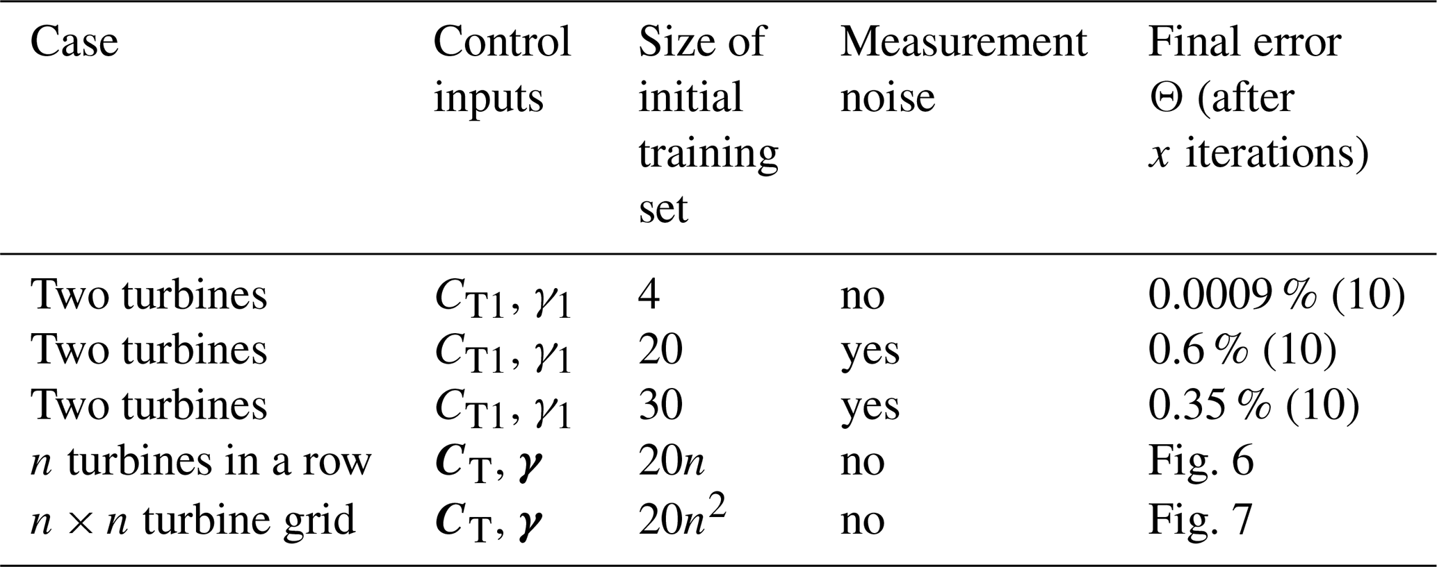
An overview of the case studies discussed in the following sections is given in Table 1.

Table 1 Overview of the case studies.

4.1 Two-turbine case

The operating points of two turbines in a row are optimized. The thrust and yaw angle of the downwind turbine are fixed resulting in only two optimization variables in the MA–GP approach. The downwind turbine is operated at its greedy operation point. The turbine row is facing the wind and the spacing between turbines is 5 D. The power production of the wind farm in dependency of the control inputs of the upwind turbine in shown in Fig. 3. The optimal operation point of the plant is $C_{\mathrm{T},\mathrm{p}}=\mathrm{0.82}$ and γ_p=31^∘ and of the approximate model is $C_{\mathrm{T},\mathrm{p}}=\mathrm{0.89}$ and γ_p=29^∘. Indeed, the relative optimization error in the model is only Θ=1.67 %. Still, the model assumes that the power production is much less sensitive to changes in the yaw angle, which should be corrected by the MA–GP approach.

Four training points at C_T=[0.4, 0.8]^T and γ=[0, 25^∘]^T are used to create the initial training set of the GP regression model. The power production of the corrected model in dependency on the control inputs is shown in Fig. 4a. The contour plot of the objective function of the plant, approximate model and MA–GP model after the initial training is shown in Fig. 4b. Clearly four operating points are not sufficient to correct the approximate model correctly. In fact, the optimal operating point of the MA–GP model has an error of 2.87 %, which is larger than the original error in the approximate model.

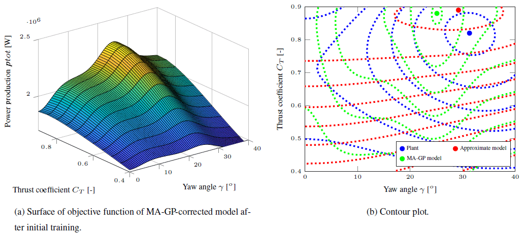
Figure 4 The power production of the MA–GP model in dependency on the control inputs of the upwind turbine and the contour plot of the plant, approximate model and MA–GP model after the initial training.

The MA–GP approach is initialized at the optimal operating point of the approximate model. In each iteration the hyperparameters and the data set of the GP regression model are updated. The new operating point is filtered with Eq. (4) and L=diag(0.4, 0.4). The MA–GP approach is able to correct the approximate model and drive the process to its optimal operating point (Fig. 5). After four iterations the relative error Θ is about 0.2 %, and after 10 iterations it is 0.0009 %. In addition, the contour lines of the objective function are well approximated (Fig. 5). A larger difference between the MA–GP model and the plant can be observed at the edges away from the current operating points. Data points at the edges are necessary to improve the identification there. However, to drive the process to its optimal operating points a correct identification of the objective function far away from the maximum is unnecessary. Clearly the initial training set with only four operating points could be increased to improve the identification of the initial model of the MA–GP approach.

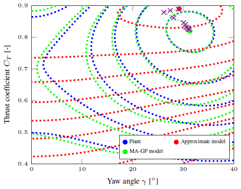
Figure 5 The contour plot of the plant, approximate model and MA–GP model after 10 iterations. The operating points of each iteration are marked with a cross.

In the current example it was assumed that the measurements are noise-free. If noise is added to the power measurements, the correct identification becomes more challenging and a larger training data set is necessary. A noise with a standard deviation of 50 kW is added to the measurement, which in the current setup translates to a turbulence intensity of about 3 %. The standard deviation is of the same size as the error in the power production of the plant and approximate model at the optimal operating point of the plant. A training data set of 20 points is created. After 10 iterations the relative error Θ is about 0.6 %. The algorithm is able to converge. However, due to the measurement noise a small error remains after 10 iterations. The error can be easily decreased with a larger initial data set; e.g., with a training set of 30 points the error after 10 iterations is about 0.35 %.

4.2 The n turbine row case

In this subsection the optimization of n turbines aligned in a row with a spacing of 5 D is discussed. It is difficult to know the required size of the training set for a satisfying performance of the MA–GP approach a priori. It depends on the sensitivity of the output to the input variables. It is, however, recommended to have about 10 training points for each input (Loeppky et al., 2009). Therefore, the size of the initial training set is chosen to be n_d=10n_u, where n_u is the number of control inputs. The operating points of the training set are chosen randomly using Latin hypercube sampling. The convergence of the MA–GP algorithm is tested on 25 Monte Carlo simulations. The difference between each run is the initial training set.

The error increases with the number of turbines, while it is almost zero for two to four turbines (Fig. 6). A reason for the increase in the error with more turbines is the similar sensitivity of the control inputs of each turbine to the power output of the plant. It makes it challenging to correctly identify the input–output map. The error can be decreased with more data in the training set. Currently, the optimization of the process and the optimization of the hyperparameters take less than a second even for the 10-turbine case. Consequently, it is possible to increase the size of the training data set for the GP regression if more data points are available.

Figure 6 (a) The boxplot of the optimization results for the differently long wind turbine rows on the left. The red line indicates the median. The bottom and top edges of the blue box indicate the 25th and 75th percentiles, respectively. The red markers indicate outliers, and the whiskers extend to the most extreme data points not considered as outliers. The error in the MA–GP approach and the initial error are dependent on the number of turbines in the row. (b) The initial error in the model depending on the number of turbines in the row.

Assuming a sufficiently large initial training set, the MA–GP approach is able to find the near-optimal point in one iteration since the approach basically just improves the surrogate model. This stands in contrast to purely model-free approaches, e.g., extremum seeking (Johnson and Fritsch, 2012) or maximum power point tracking (Gebraad et al., 2013), which usually need several iterations to find an optimum. Moreover, after the initial training, the MA–GP model usually represents the plant better than the approximate model. Nonetheless, measurements close to the optimum of the MA–GP model can help to improve the model further.

4.3 The n×n turbine grid case

In this subsection the optimization of a wind farm with turbines arranged in an n×n grid with a spacing of 5 D is presented. Consequently, the wind farm consist of n turbine rows each containing n turbines. The wind direction is aligned with the rows of the grid. Interaction between parallel rows is neglectable, and is, in any case, not known to the MA–GP approach. Again the size of the initial training set is chosen to depend linearly on the number of control inputs with n_d=10n_u and the MA–GP approach is tested on 25 Monte Carlo simulations.

Again the algorithm converges for a small number of turbines (Fig. 7a). However, the error in the optimization increases as the number of turbines increase. Moreover, for grids with 25 and more turbines the majority of the optimizations become stuck at the initial conditions, which are defined by the optimal operation point of the model (Fig. 6b)¹. This behavior might be caused by overfitting causing multiple local optima in the MA–GP model. Moreover, even in the cases where the MA–GP approach improves the performance of the wind farm, the algorithm converges to errors in the range of 1 %–2 % after 25 iterations. These are much larger than observed in the turbine row case.

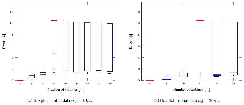
Figure 7 The boxplot of the optimization results for the differently sized wind turbine grids. The red line indicates the median. The bottom and top edges of the blue box indicate the 25th and 75th percentiles, respectively. The red markers indicate outliers, and the whiskers extend to the most extreme data points not considered as outliers. The error in the MA–GP approach and the initial error are dependent on the number of turbines in the row. The difference between both runs is the size of the initial training set.

If the MA–GP algorithm for larger wind farms converges to an optimum, it usually first takes a few iterations, where the wind farm is operated at the optimal point of the approximate model, before the error reduction begins. Obviously the algorithm needs the additional information around the operating point. Interestingly, once the algorithm actually leaves the initial operating point, it converges relatively quickly to an operating point close to the plant optimum. This is a strong indication that exploration or even just small excitation around an operating point should be activated if the operating point does not change for some time.

A reason for the increase in the error in larger wind farms is the decrease in the sample density. The size of the initial training set is increased linearly, while it would have to increase exponentially to preserve the same sampling density. For the wind farm with 100 wind turbines and the current setup, the hyperparameter optimization usually takes about 15 s. In some rare cases it took about 5 min. In these cases the optimizer was not able to converge to an optimum and the maximum number of allowed iterations were used. The plant optimization takes less than 10 s. Consequently, the size of the data set is not a limiting factor in improving the performance of the larger wind farms.

The increase in the initial training set improves the convergence of the method (Fig. 7b). Nevertheless, even with the larger size of the initial training set, it is challenging to converge to the correct optimum point for cases with a large input space. A larger training set would be necessary for these cases. On the other hand, the training of the hyperparameters in the GP regression scales cubically with the number of data. Obviously this ultimately limits the size of the training set since the approach can become computationally infeasible.

Nonetheless, the results show clearly that the MA–GP approach is able to improve the performance of the model-based optimization for some of the cases. It is not clear how the initial data sets differ for these successful cases. However, it is expected that a large number of operation points can be excluded from the initial training set of the GP regression since it is known from the model that they are far away from the optimum operating point. Currently, the initial training set is chosen randomly by Latin hypercube sampling. A smarter selection with a larger density of points around the optimal operating point of the model may improve the MA–GP approach without increasing the initial data set.

In the next section the practical implications of the MA–GP approach are discussed.

5 Discussion

In this section an outlook on how to apply the MA–GP approach to a real wind farm is given. It is beyond this article to solve all the associated challenges.

A major challenge is the dynamic environment a wind farm operates in. Averaging and filtering is required to approximate steady-state conditions. In a nine-turbine large-eddy simulation (LES) study presented in Andersson et al. (2020c)², 5 min averaging is used. A longer averaging horizon will make the MA–GP more robust since the variance in the data decreases. A too long averaging horizon will reduce the performance since the plant response is delayed and averaged. Moreover, measurement and input noise can degrade the performance of the adaptation. The negative influence of input and measurement noise can be reduced by a larger training data set.

Another challenge is the wake propagation delay. In the LES study the first 5 min after a change in the control inputs is discarded to remove the transients. A similar approach might be necessary in a real wind farm. A wake propagation through the entire farm is not necessary. Depending on the measurements noise level it suffices to include the interaction of about two to three turbines (Andersson et al., 2020a).

The sensitivity of the input–output map can be increased by including the power measurements of each turbine and identifying a multiple-input multiple-output model. It is shown in Andersson et al. (2020a) that this can help to decrease the necessary size of the training data set and improve the performance of the MA–GP approach for large wind farms. In addition, the wind farm could be separated into subsets. The separation would depend on the turbines' interaction considering a range of wind directions, e.g., a wind farm as presented in Sect. 4.3 could be separated into several subsets for each of the wind directions around 0, 45, 90, 135, 180, 225, 270 and 315^∘.

For a real wind farm the minimum training set should contain wind velocity, wind direction, the control inputs and the plant–model error in the power outputs of each turbine. The inclusion of other variables, e.g., the turbulence intensity, depends highly on the sensitivity of the variable to the plant–model mismatch of the power productions. Their effect should be larger than the effect of the input noise of the wind. Otherwise, it is not recommended to include them in the MA–GP approach.

Atmospheric conditions that considerably change the response of the wind farm could be handled by a multimodel approach. The model error for each atmospheric condition is identified using a separate model. The multimodel approach can also be used to estimate the current atmospheric conditions. If the atmospheric conditions are not considered explicitly in the MA–GP approach the response of the wind farm will be averaged over the atmospheric conditions. In fact, this happens to every variable that is not explicitly considered. On the other hand, the MA–GP approach automatically adapts to constant effects, e.g., terrain effects.

It is important to point out that the MA–GP approach supplements model-based wind farm control. It is still beneficial to have a good wind farm model even though theoretically the MA–GP approach can work with a poor wind farm model. Moreover, the initial training set of the MA–GP approach can be generated by a high-fidelity model. In that case the MA–GP approach would initially reduce the error between the surrogate and high-fidelity model, which should improve the performance of the wind farm controller. During operation the initial data set can be gradually replaced by real measurements. The GP allows for the weighting of different training sets, which should be used when working with two different training sets. Moreover, during operation the data set should be updated, continuously replacing old data points with new ones.

The initial synthesis of the MA–GP approach can be similar to the approach presented in Doekemeijer et al. (2020):

1. create training data set using high-fidelity simulations;

2. estimate the model parameters of the approximate model using high-fidelity data;

3. identify a model of the plant–model mismatch of the approximate and high-fidelity model using GPs.

If during operation the free-stream wind velocity or the turbulence intensity are also estimated, only the approximate model without the MA–GP correction should be used to avoid a feedback of the identified model into the training set.

6 Conclusions

The modifier adaptation approach with Gaussian processes applied to wind farm control is presented. It is a real-time optimization strategy, which corrects the approximate model used in the optimization by using plant measurements. In the wind farm case the total power production is assumed to be measured and used in the MA–GP approach. The approach works well for small input spaces. Here the GP regression is able to correct the model almost perfectly. Consequently, operating points very close to the real optimum are found in the optimization. For larger input spaces, on the other hand, the error increases. Moreover, for the grid-type wind farm layout with more than 25 turbines, convergence with the relatively small initial training sets used in this work could not be achieved at all times.

The MA–GP approach has similarities with Bayesian optimization (BO). Park et al. (2016, 2017) applied BO successfully in wind tunnel tests, and we expect the MA–GP approach to behave similarly. In Sect. 5 several possible future investigations to make the MA–GP approach applicable to real wind farms were pointed out. The performance of large wind farms can be improved by the multiple input and multiple output approach and subset separation. In addition the following ideas can be tested:

• Increase the training set until it becomes computationally unfeasible to increase the training set further.

• Choose the training data points in a smarter way such that they provide enough information about the regions around the expected optimum. Operating points far away from the expected optimum are excluded.

• Extend the algorithm with an exploration part. This can be achieved, for example, by including the variance in the GP regression model in the optimization.

An important investigation is the sensitivity of the approach to measurements, input noise and time delays. In Andersson et al. (2020b) a simple way to include input noise explicitly in the MA–GP approach is presented. Finally, the model identification should be tested on high-fidelity and real data. A preliminary study on a nine-turbine wind farm case using data from the high-fidelity simulator SOWFA (Churchfield et al., 2012) will be presented in Andersson et al. (2020c).