the Creative Commons Attribution 4.0 License.
the Creative Commons Attribution 4.0 License.
 | 22 Jul 2020
The flow past a flatback airfoil with flow control devices: benchmarking numerical simulations against wind tunnel data
George Papadakis
Marinos Manolesos
As wind turbines grow larger, the use of flatback airfoils has become standard practice for the root region of the blades. Flatback profiles provide higher lift and reduced sensitivity to soiling at significantly higher drag values. A number of flow control devices have been proposed to improve the performance of flatback profiles. In the present study, the flow past a flatback airfoil at a chord Reynolds number of 1.5×10⁶ with and without trailing edge flow control devices is considered. Two different numerical approaches are applied, unsteady Reynolds-Averaged Navier Stokes (RANS) simulations and detached eddy simulations (DES). The computational predictions are compared against wind tunnel measurements to assess the suitability of each method. The effect of each flow control device on the flow is examined based on the DES results on the finer mesh. Results agree well with the experimental findings and show that a newly proposed flap device outperforms traditional solutions for flatback airfoils. In terms of numerical modelling, the more expensive DES approach is more suitable if the wake frequencies are of interest, but the simplest 2D RANS simulations can provide acceptable load predictions.
- Article
(9189 KB) - Full-text XML
- BibTeX
- EndNote


Wind turbine blade design is dominated by structural and transportation requirements in the root region, which results in compromised aerodynamic design. This leads to the use of thicker airfoils with a blunt trailing edge (TE), i.e. flatback (FB) airfoils, in the inner part of the blade. This design option is becoming more and more popular as wind turbines grow larger and rotor diameters go beyond 200 m.
FB airfoils provide a number of aerodynamic, structural and aeroelastic benefits compared to traditional airfoils of the same thickness. Aerodynamically, they provide higher lift values due to the reduced adverse pressure gradient over the aft part of the suction side. Additionally, their performance is insensitive to surface roughness compared to traditional airfoils of similar thickness (Baker et al., 2006). Structurally, they have larger cross-sectional area and can lead to significant blade weight reduction (Griffith and Richards, 2014). Blades that utilise FB profiles also have improved aeroelastic behaviour, as the blunt TE offers increased flap-wise stiffness.
The performance of FB profiles can be further improved by means of various TE add-ons, which alter the unsteady bluff body wake that forms downstream of the blunt TE. TE devices extend the vortex formation length at the wake of the blunt TE (Manolesos et al., 2016a) and lead to the increased base pressure and Strouhal number of the flow fluctuations in the wake. At the same time, the amplitude of the flow fluctuations is reduced, reducing the danger of vortex-induced vibrations for wind turbine blades and also reducing noise (Barone and Berg, 2009).
Numerical study of the flow past FB airfoils is particularly challenging due to its unsteady and three-dimensional (3D) nature, which includes impingement, separation and vortex shedding. Prediction of force coefficients and wake characteristics depend heavily on the fidelity of the numerical approach, the mesh resolution and the size of the domain (Calafell et al., 2012; Lehmkuhl et al., 2014; Stone et al., 2009). It is generally agreed that two-dimensional and Reynolds-Averaged Navier Stokes (RANS) simulations non-physically damp the flow (Stone et al., 2006) and that higher-fidelity approaches might be more suitable (Standish and Van Dam, 2003), especially if the flow frequencies in the wake are of interest. There have been a number of investigations at high Re numbers (Calafell et al., 2012; Kim et al., 2014; Lehmkuhl et al., 2014; Standish and Van Dam, 2003; Stone et al., 2009; Xu et al., 2014). However, most deal with 2D or low-aspect-ratio simulations and not with TE devices for flow control.
The highest-fidelity simulations to date remain those of Hossain et al. (2013), who performed Direct Numerical Simulation (DNS) on a FX77-W-500 airfoil, albeit using a very low Re number of Re=3900.
As far as bluff body drag reduction is concerned, it has been an active area of research for decades (Choi et al., 2008; Tanner, 1975; Viswanath, 1996). The most commonly applied technique to reduce base drag is the alteration of the TE shape, either by means of afterbody modification or by 3D shaping of the TE. The common aim is to increase base pressure by modifying the vortex shedding in the wake. Studies on flatback airfoils (Baker and Van Dam, 2009; Kahn et al., 2008; Krentel and Nitsche, 2013; Mayda et al., 2008; Nash, 1965) have highlighted using a single splitter plate or a pair of plates, forming a cavity at the TE, as an extremely simple and effective method.
The present investigation deals with the flow past a 30 % thickness wind turbine airfoil with a 10 % thickness blunt TE (Boorsma et al., 2015) at a Reynolds number of . The corresponding Reynolds number based on the blunt TE thickness is . It is the continuation of an experimental survey that examined a number of TE devices to improve the performance of the profile (Manolesos and Voutsinas, 2016b). That work was a proof-of-concept study for a FB airfoil flap device, which proved to perform better than traditional devices.
The objective of the present study is (a) to examine which numerical approach is most suitable for the study of the flow in question and (b) to provide insight into the effect of the various flow control devices on the airfoil wake. It is noted that the study is limited to extruded airfoils with no twist or profile change, and extension of any findings to 3D rotating blades would require further validation. The next section presents the methodology followed in this study. Subsequently, the results are presented and discussed, while the final section concludes the findings of this investigation.
2.1 Numerical set-up
All simulations were performed using MaPFlow (Papadakis and Voutsinas, 2019), the Computational Fluid Dynamics(CFD) solver developed at NTUA's Aerodynamics Laboratory. In the present case, the Eulerian module of MaPFlow was used, which is a compressible cell-centred CFD solver that can use both structured and unstructured grids. Turbulence closures implemented on MaPFlow include the one-equation Spalart–Allmaras (SA) turbulence model (Spalart and Allmaras, 1992) and the two-equation turbulence model of Menter, k-ω Shear Stress Transport (SST), (Menter, 1993). The improved delayed detached eddy simulation (IDDES) approach implemented in MaPFlow follows the suggestions of Shur et al. (2008). The IDDES model considers a RANS zone in the boundary layer region and switches to Large Eddy Simulation (LES) in the wake.
The IDDES model definition for the local length scale Δ used in the current work is as follows:
where Cw is an empirical constant, hwn is the mesh step in the wall normal direction and . For Cw, the value of 0.15 is chosen.
The switch from RANS to IDDES is accomplished by altering the distance from the wall used in the original model according to the following equation:
where lRANS is the distance from the wall (original SA model) and lLES=CDESΨΔ, where CDES is an empirical constant and Ψ is a low Reynolds number correction (for details, see Shur et al., 2008)
In the present study, 2D and 3D simulations using the unsteady RANS approach with the SA turbulence model and the IDDES method were performed. For the 3D results, two grids of different spatial resolution were generated. The grids were hybrid, i.e. structured close to the airfoil and unstructured far from it. Figure 1 shows the coarse and the fine grids, along with the grid used in the stereo particle image velocimetry (PIV) measurements for comparison. The coarser grid consisted of 5 million cells, while the finer contained 25 million cells. The fine 25 million cell grid for the offset cavity case is also shown for reference. The computational domain extended for one chord length in the spanwise direction, i.e. much wider than the spanwise coherence in the wake, which has been found to be ∼5 TE heights (Metzinger et al., 2018). The reason for this is that the present study will be extended to higher angle of attack (AOA), where Stall Cells (SC) (Manolesos et al., 2014a, c) appear on flatback airfoils (Manolesos et al., 2014b; Manolesos and Voutsinas, 2016b). For the accurate computation of these large structures, high-aspect-ratio (AR) computational domains are necessary. Symmetry conditions were applied at the side boundaries of the computational domain. For the coarser grid, 60 nodes were used in the spanwise direction, while 200 were defined for the finer grid. The grids were refined in all directions to ensure that the computational cell aspect ratio in the wake remained close to unity. Regarding the far-field boundary, it was located 100 chords away from the wing to minimise the influence of the external boundary conditions on the simulations (Sørensen et al., 2016). The same computational mesh was used for both URANS and DES simulations to exclude grid-related differences. For the 2D URANS simulations, a slice of the coarse grid was used, which had 88 k cells. All simulations were performed at an AOA . All of the simulations consider the flow fully turbulent to exclude possible uncertainties related to transition modelling.
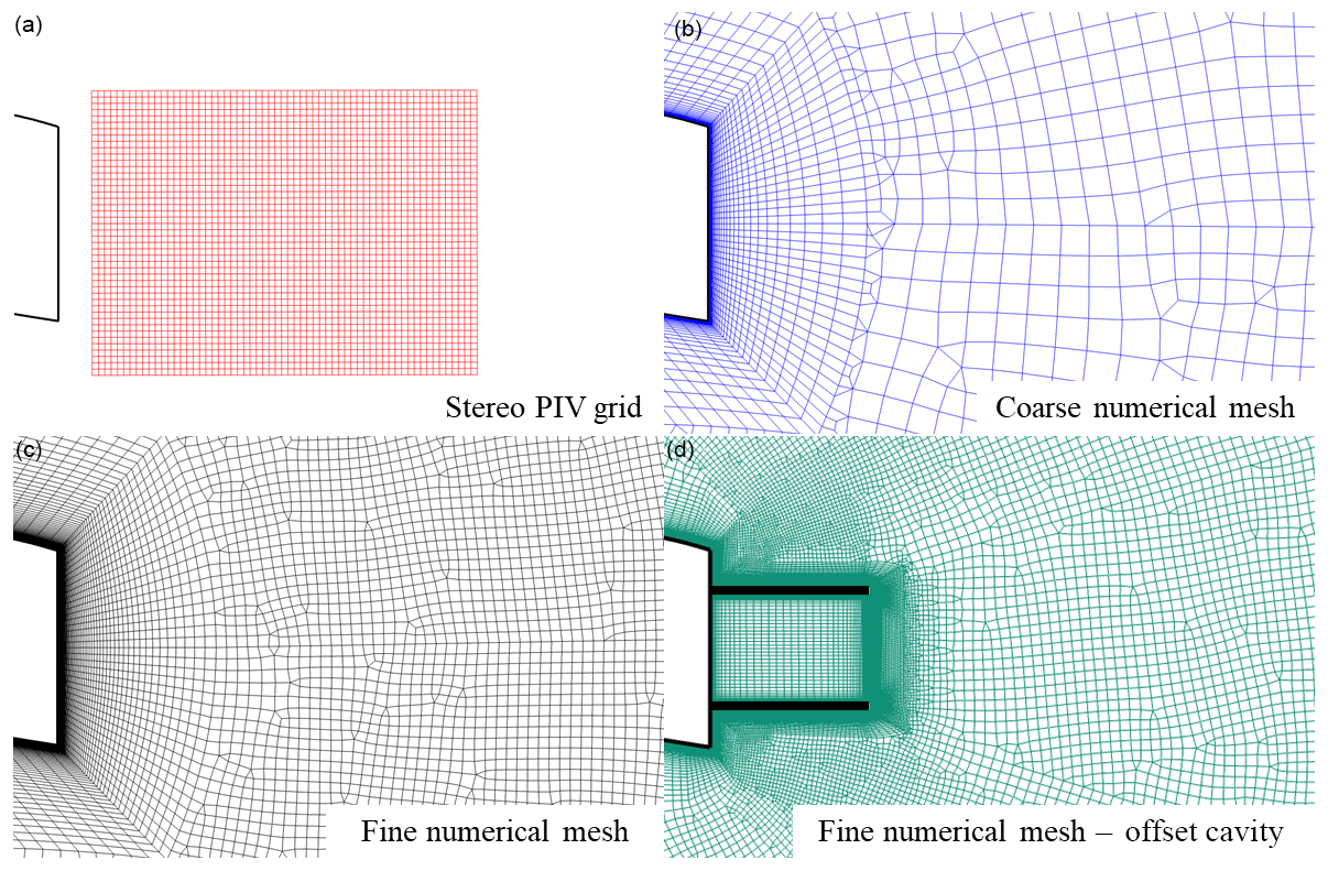
Figure 1Details of the stereo PIV grid and the numerical meshes: (a) stereo PIV measurement grid, (b) coarse numerical mesh (5 million cells), (c) fine numerical mesh (25 million cells), and (d) fine numerical mesh for the offset cavity case (25 million cells).
2.2 Experimental set-up
The numerical results are compared against stereo particle image velocimetry (PIV), force coefficients and hot-wire measurements in the wake of the airfoils. In the experiments, the wing model had a chord of c=0.5 m and an aspect ratio of AR =2. Figure 2 presents a schematic of the measurement set-up, where the stereo PIV measurement plane is shown, along with the location of the hot-wire probe in the wake of the airfoil. Extensive details of the wind tunnel tests can be found in (Manolesos and Voutsinas, 2016b).
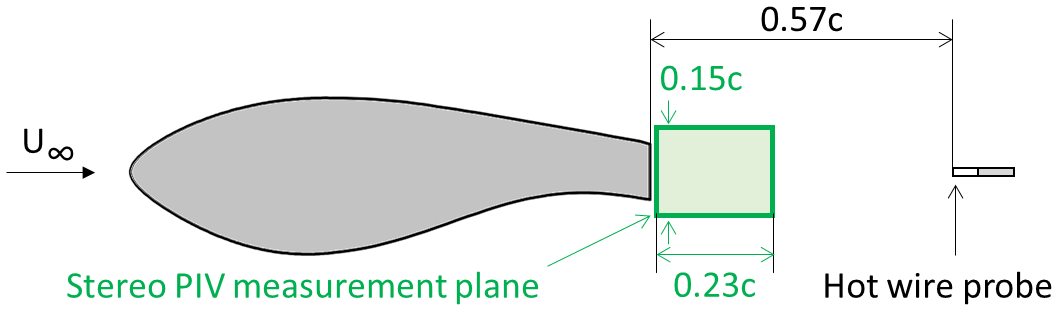
Figure 2Schematic of the experimental set-up, showing the flatback airfoil under investigation, LI30-FB10, the location of the hot-wire probe in the wake, and the size of the stereo PIV measurement plane.
All cases concern a 30 % thickness FB airfoil with a 10.6 % thickness TE (LI30-FB10 Boorsma et al., 2015, Fig. 2), which was tested at . The four best performing devices tested by Manolesos and Voutsinas (2016b) are considered in the present investigation, as shown in Fig. 3. Only free-transition experimental results were available for these cases. The splitter and the offset cavity are traditional devices studied by a number of researchers (e.g. Kahn et al., 2008; Viswanath, 1996). The flap and the flap + offset cavity devices were proposed in a proof-of-concept study (Manolesos and Voutsinas, 2016b). The TE thickness was hTE=53 mm, while the splitter and offset cavity lengths were 0.81hTE. The offset cavity plates were located 0.19hTE from the TE edges. The flap had a chord of 0.62hTE and was located at 20∘ with respect to the airfoil chord. Its TE was at 0.75hTE downstream of the airfoil TE.
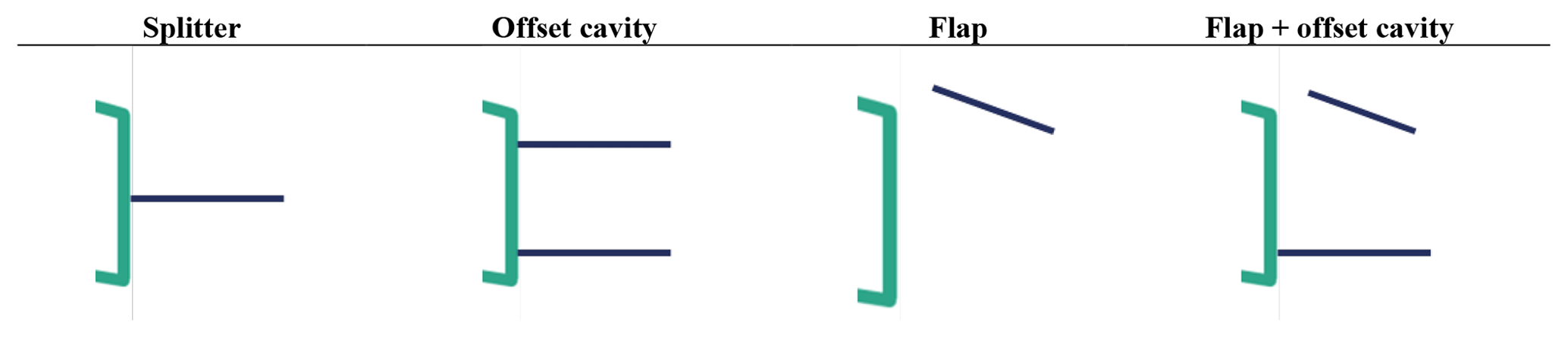
Figure 3Close-up detail of the blunt trailing edge with the four devices considered in this study.
A detailed uncertainty analysis can be found in Manolesos and Voutsinas (2016b), but a short overview is given here for completeness. The 95 % confidence intervals for the lift and drag values are 1 % and 4 %, respectively. For the hot-wire frequency spectrum, the frequency step was 1.95 Hz, while for the stereo PIV measurements the minimum resolvable velocity is 1.5 % V∞. Any velocities lower than this should not be trusted. A constant misalignment of the model has been allowed for in the results. In the remainder of this article all quantities are non-dimensionalised using the chord and the free-stream velocity, V∞, as reference values, unless otherwise stated.
Given the large amount of numerical and experimental data, only a selection are presented in this report. First, the numerical predictions are compared against the measurement data in terms of force coefficients, wake frequencies and amplitudes. Then the time-averaged stereo PIV data are compared against the simulation results. The coarse and fine URANS and IDDES results are included in these comparisons to assess which method is the most suitable for the analysis of the flow under investigation. The 2D URANS data are also included for reference. Finally, the most suitable method, IDDES on the fine mesh, is used to examine the flow mechanisms introduced by the flow control devices at the TE of the wing.
3.1 Comparison with experimental data
3.1.1 Force coefficients
Figure 4 compares the lift and drag coefficient predictions with the relevant experimental values, while the glide ratio (L∕D) comparison is given in Fig. 5. The error bars are based on the standard deviation values. For completeness the relevant values are also given in Tables A1 and A2 in the Appendix. In terms of mean values, the agreement is good in qualitative terms and all methods capture the trends for lift and drag and the lift-to-drag ratio (L∕D). In quantitative terms, predictions are significantly better for lift than for drag, in agreement with previous studies (Stone et al., 2009; Xu et al., 2014). As far as comparative performance is concerned, all simulations, even the lowest-fidelity 2D RANS, agree with the experiments and suggest that the airfoil with the flap would produce the highest lift and the highest lift-to-drag ratio; see Fig. 5.
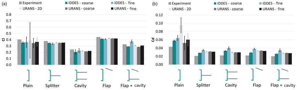
Figure 4Lift (a) and drag coefficient (b) values for the plain airfoil and the airfoil with different TE devices: comparison between experiments, IDDES simulations and URANS simulations. Error bars in the numerical predictions are equal to the standard deviation of the force coefficient.
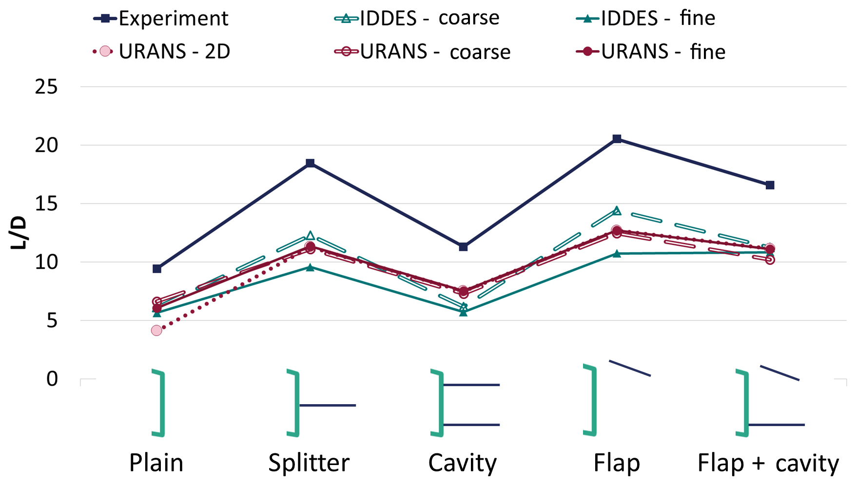
Figure 5Lift-to-drag ratio for the plain airfoil and the airfoil with different TE devices: comparison between experiments, IDDES simulations and URANS simulations.
With regards to load variation (denoted by the error bars for the lift, Cl, and drag, Cd, coefficients in Fig. 4), only the highest-fidelity method, IDDES on the fine mesh, predicts unsteady forces for all cases with or without the TE devices. There are no experimental data for the load variation, but stereo PIV and hot-wire velocity measurements indicated significant flow variation in the wake, so it is expected that forces on the wing should vary as well.
With regards to the different methods, URANS predictions are significantly affected by the change from 2D to 3D. The 2D simulations overpredict drag, as they restrict a naturally 3D flow to be 2D (Metzinger et al., 2018; Xu et al., 2014). This leads to very high load fluctuations, especially for the plain airfoil case. As the wake analysis in the following section indicates, the shed vorticity remains coherent, and thus the induced forces are overpredicted. On the contrary, URANS simulations, whether 2D or 3D, do not predict any load fluctuations for the cases with the TE devices. It appears that URANS artificially damps the flow, regardless of the dimensions or the spatial resolution when TE devices are employed.
Mesh resolution appears to play an important role for IDDES, more so than for URANS. URANS predictions remain practically unchanged moving from the coarse to the fine mesh, especially for the TE device cases. IDDES predicts higher drag values with the fine mesh, and, more importantly, the fine IDDES simulation is the only one that predicts unsteady forces for all cases. Regarding URANS, unsteady forces are only predicted for the Plain airfoil case. The 2D URANS predicts significantly higher forces, a result of confining an inherently 3D flow within two dimensions.

Figure 6Normalised power spectral density of the velocity time series for the plain airfoil and all the TE device cases from fine IDDES simulations. The vertical velocity is considered at ; see also Fig. 2. Strouhal number is defined based on the trailing edge thickness, .

Figure 7(a) Strouhal number ( values for the plain airfoil and the airfoil with different TE devices: comparison between the experiments, IDDES simulations and URANS simulations. (b) Normalised peak amplitude of the frequency spectrum: comparison between experiments and fine IDDES simulations.
3.1.2 Wake frequencies
Figure 7a presents the Strouhal number values, comparing the experiments, IDDES simulations and URANS simulations. The St number is calculated based on the TE thickness and the main frequency, f, according to the equation below:
In the wind tunnel data, frequency, f, is the main frequency in the velocity spectrum from the wake hot-wire measurements (see also Fig. 2). Similarly, for all simulations the velocity time series at the location of the hot-wire probe was examined and the dominant frequency from the vertical velocity spectrum was taken. Figure 7b shows the normalised peak amplitude of that frequency, Anorm, according to Eq. (4):
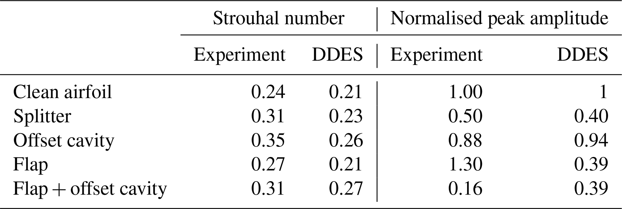
where Aplain is the amplitude of the dominant frequency for the plain airfoil case. Table 1 presents the relevant values (St and Anorm) for the experiments and the highest-fidelity simulation, fine IDDES. The power spectral density (PSD) for the fine IDDES cases is given in Fig. 6.
In case of the plain airfoil, all St predictions are close to the experimental results but are lower, in agreement with Stone et al. (2009). Increasing the mesh size from 5 to 25 million leads to improved IDDES predictions for all cases. For RANS, the wake frequency is practically insensitive to mesh resolution or dimensions (2D or 3D). The results show that URANS fails to predict the wake unsteadiness in the case of the TE devices or provides erroneous predictions (URANS fine, URANS splitter).
A closer look at the comparison between the experiment and the fine IDDES simulation results (Fig. 7, right and Table 1) reveals that IDDES can qualitatively predict both the frequency and the normalised peak amplitude, suggesting that the main flow mechanisms are correctly captured by the selected approach. The largest difference is observed for the flap and flap + offset cavity cases. At this point the reason for this discrepancy remains unclear. It is noted, however, that during the experiments the flap, which was manufactured out of a 2 mm thick aluminium sheet, was slightly deflected under the aerodynamic load. It was not possible to quantify the deflection or its effect at the time. Interestingly, IDDES predictions regarding the velocity's fluctuation frequency are in fair agreement with the experimental data for all configurations even when the coarser grid is employed.
According to Manolesos and Voutsinas (2016b), the wake contains structures of smaller size and higher frequency when the TE devices are used. The velocity spectrum from the IDDES simulations (Fig. 6) agrees with this observation, except for the flap case, where the St number is the same as for the plain airfoil case. It is conceivable that this is because the vortex shed from the lower edge of the blunt TE is unaffected by the presence of the flap, as discussed in Sect. 3.2.
Table 1Strouhal number () and normalised peak amplitude of the frequency spectrum for the plain airfoil and the airfoil with different TE devices: comparison between experiments and IDDES simulations.
3.1.3 Wake velocity and turbulence quantities
In this section the time-averaged velocity magnitude as measured on the stereo PIV plane is compared with the numerical predictions on the fine mesh. In the interest of brevity, only the normal Reynolds stress is presented from the turbulence quantities, but it is noted that the same conclusions can be reached by examining the other quantities. Figures 8 to 12 present the relevant contours for all the examined cases.
In the plain airfoil case (Fig. 8), where both URANS and IDDES predict significant vortex shedding, the velocity contours are very similar, with the IDDES prediction closer to the wind tunnel data. In all cases, the mean velocity wake initially becomes thinner (as highlighted by the black arrows in Fig. 8) before expanding further downstream. This is linked to the roll up of the two shear layers into discrete vortices that are shed in the wake. The recirculation region compares well between experiments and simulations, with numerical prediction of the recirculation length being similar to the measured one.
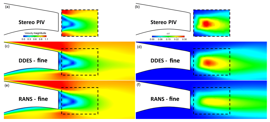
Figure 8Plain airfoil case. Normalised velocity magnitude contours, V∕V∞, (a, c, e) and normal Reynolds stress contours (b, d, f): comparison between stereo PIV, RANS and IDDES results. The fine mesh (25 million cells) was used in the calculations.
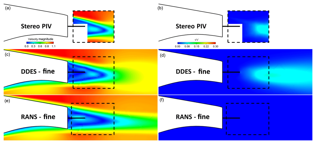
Figure 9Splitter case. Normalised velocity magnitude contours, V∕V∞, (a, c, e) and normal Reynolds stress contours (b, d, f): comparison between stereo PIV, RANS and IDDES results. The fine mesh (25 million cells) was used in the calculations.
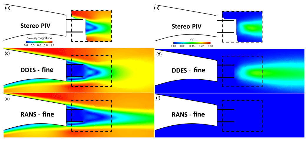
Figure 10Offset cavity case. Normalised velocity magnitude contours, V∕V∞, (a, c, e) and normal Reynolds stress contours (b, d, f): comparison between stereo PIV, RANS and IDDES results. The fine mesh (25 million cells) was used in the calculations.
Contrary to mean velocity contours, the Reynolds stress predictions differ to some extent with the URANS-predicted values being smaller than the IDDES and the experimental ones. Again, there is a very good agreement between the latter two. The IDDES velocity fluctuation peaks appear at the same locations as in the experiments, which means that the vortex formation length (Tombazis and Bearman, 1997; Williamson, 1996) is also predicted correctly.
In all other cases (splitter, offset cavity, flap, flap + offset cavity) the URANS simulations do not predict vortex shedding. As a result, the recirculation region is significantly longer than in the wind tunnel tests and Reynolds stress values are close to zero everywhere. Additionally, the lack of mixing in the wake means that low velocities are maintained in the wake further downstream. This is not in agreement with the experimental measurements or the IDDES predictions, where vortex shedding is observed along with significant Re stress values and quicker wake recovery.
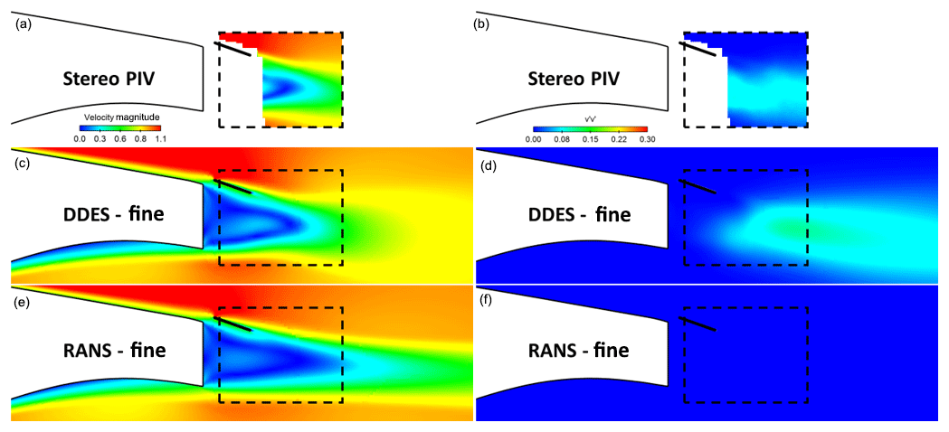
Figure 11Flap case. Normalised velocity magnitude contours, V∕V∞, (a, c, e) and normal Reynolds stress contours (b, d, f): comparison between stereo PIV, RANS and IDDES results. The fine mesh (25 million cells) was used in the calculations.
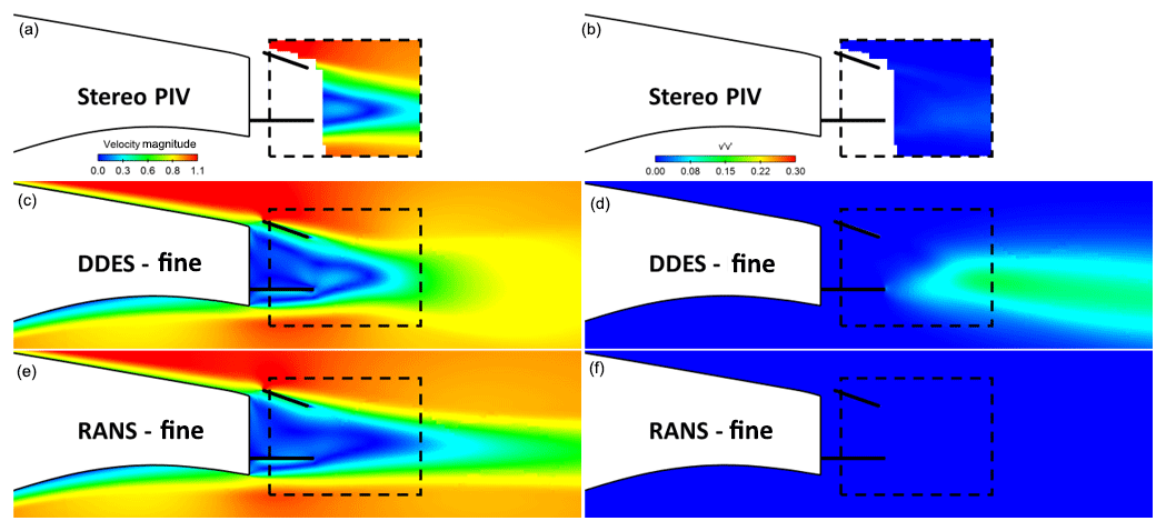
Figure 12Flap + offset cavity case. Normalised velocity magnitude contours, V∕V∞, (a, c, e) and normal Reynolds stress contours (b, d, f): comparison between stereo PIV, RANS and IDDES results. The fine mesh (25 million cells) was used in the calculations.
Figure 12 reveals a disagreement between the IDDES Re stress predictions and the wind tunnel measurements for the flap + offset cavity case. The stereo PIV data, in agreement with the hot-wire measurements, suggest that the flow variations are significantly smaller for this case than all other cases. IDDES do predict reduced fluctuations compared to the plain airfoil case but not to the extent suggested by the measurements. This is also confirmed by the PSD graph shown in Fig. 6, where the energy contained in all frequencies of the flap + offset cavity case are lower than all other cases. However, the recirculation region and vortex formation length remain larger in the IDDES simulations than in the wind tunnel tests.
In general, the IDDES predictions are satisfactory, but the wake appears to be “wider”, or more diffused, than in the experiments. This could imply that numerical diffusion is significant even with the 25 million cell mesh and that possible improvements can be expected by a further increase in the spatial resolution.
3.2 Wake development
The analysis so far has shown that the predictions of the highest-fidelity numerical approach, IDDES on the fine mesh, are closer to the experimental data in terms of load values, wake velocities and frequencies, and turbulence quantities. Consequently, the analysis of the wake development and the effect the TE devices have on the vortex shedding mechanism will be based on the fine IDDES results. For completeness, the comparison between the URANS and IDDES fine-mesh predictions is also discussed.
Figure 13 shows a comparison between the URANS and IDDES on the fine mesh for the plain airfoil case. Instantaneous vortical structures are visualised as isosurfaces of the Δ criterion (Chong et al., 1990), coloured by streamwise vorticity. These are superimposed on isosurfaces of spanwise vorticity. The values for Δ and ωz have been chosen so that the two surfaces overlap where they both exist simultaneously. This method of visualisation was selected so that both the streamwise and the spanwise vortex strength and complexity is visualised.
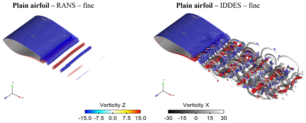
Figure 13Instantaneous isosurfaces of Δ=105 coloured by streamwise vorticity (ωx) and overlaid instantaneous isosurfaces of spanwise vorticity ().
The artificial smoothing of the flow is apparent in the case of URANS. The spanwise vortices are only mildly three-dimensional and do not give rise to streamwise braids. In the URANS predictions, a typical von Kàrmàn vortex street is formed by opposite-sign vortices arranged in an alternating fashion. However, these vortices have limited three-dimensionality and resemble wake structures of significantly lower Re number (Bai and Alam, 2018). In the present case, the Reynolds number based on TE thickness is , orders of magnitude higher than the critical Re number for bluff body wake flows (Williamson, 1996), and significant three-dimensionality is expected. The vortices in the URANS case are also very quickly damped in the wake, despite the fact that the same 25 million cell grid is used by both methods.
On the other hand, IDDES results reveal the inherently strong three-dimensional character of the flow. According to IDDES predictions, the spanwise vortices alternatingly shed from the top and bottom trailing edges of the wing, giving rise to smaller streamwise hairpin vortices. These vortices play a central role in transfer of vorticity out of the core of the main vortex (Mittal and Balachandar, 1995) and appear as soon as the vortices are shed in the wake. The latter is not surprising given the high Re number and the turbulent boundary layer over the airfoil.
Figure 14 offers the same instantaneous wake visualisation as Fig. 13 for the cases with the different TE devices, as predicted by IDDES on the fine mesh. Significant differences are observed between the various cases. Perhaps the most complicated structures appear in the splitter case, where oblique shedding is observed along with vortex dislocations (Tombazis and Bearman, 1997). Regardless, the wake remains smaller and less three-dimensional than the plain airfoil case (Fig. 13, right). In the offset cavity case, the streamwise braids appear less dense and maintain their regularity further downstream in the wake compared to the plain case. The spanwise vortices are also smaller in size and seem to break down sooner than in the uncontrolled case.
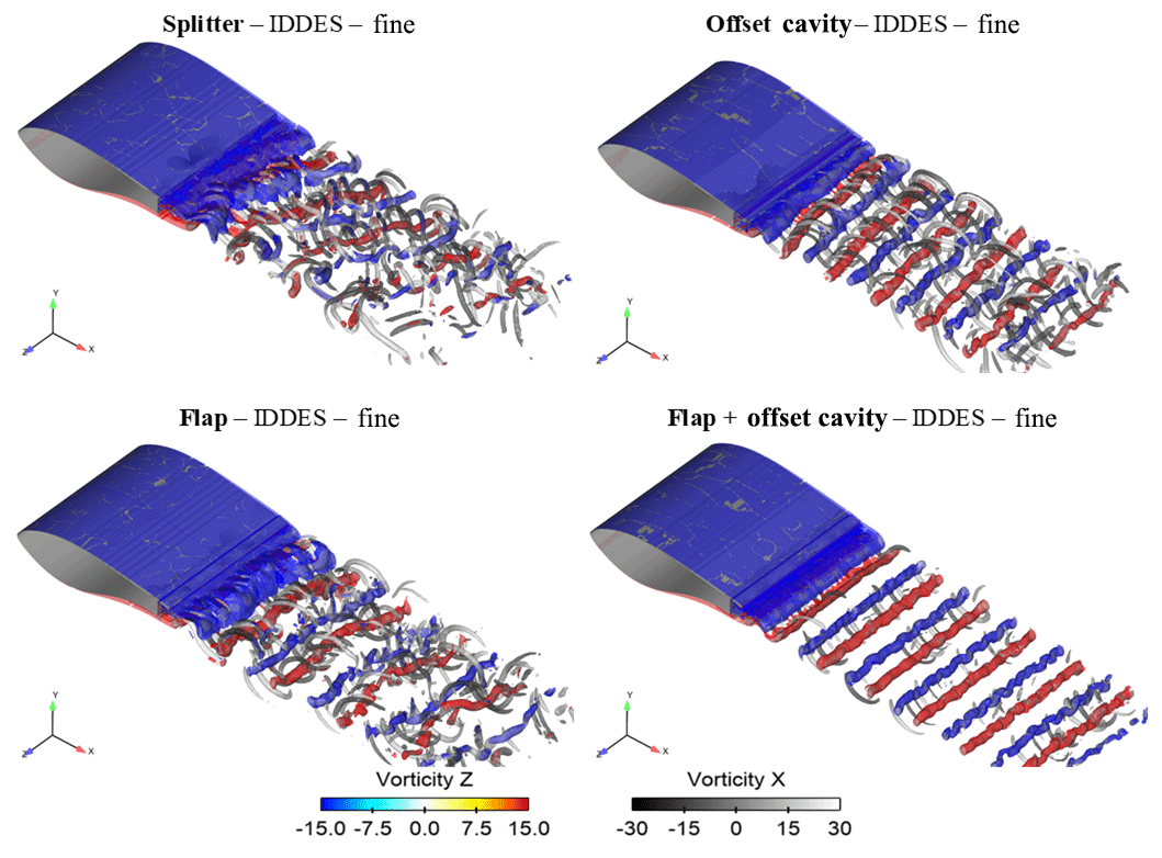
Figure 14Instantaneous isosurfaces of Δ=105 coloured by streamwise vorticity and overlaid instantaneous isosurfaces of spanwise vorticity (). IDDES results on the fine mesh.
As discussed in more detail in Sect. 3.3, in the flap case, the flap only affects the formation of the top vortex, while the lower vortex is uncontrolled by shed. The wake hence appears more irregular than in the offset cavity case, but the spanwise von Kàrmàn vortices and the streamwise vortices are clearly identifiable. The wake is significantly more regular in the flap + offset cavity case, where the lower vortex formation is affected by the presence of the cavity plate. The spanwise vortices appear to be very well structured and the streamwise braids are not as pronounced.
Based on the analysis above it can be concluded that the TE devices all affect the formation of the von Kàrmàn vortices, which are present in all cases. All controlled cases have a smaller and less turbulent wake, in agreement with the previous section and with Manolesos and Voutsinas (2016b). In general, the stronger the spanwise vortex, the stronger its three-dimensional character. Comparing the cases of splitter and offset cavity, it appears that the distance of the control plate plays a significant role in the vortex formation and strength. Finally, the comparison between the flap and the flap + offset cavity cases suggests that controlling only one side of the vortex street is not sufficient to create a well-structured and less turbulent wake.
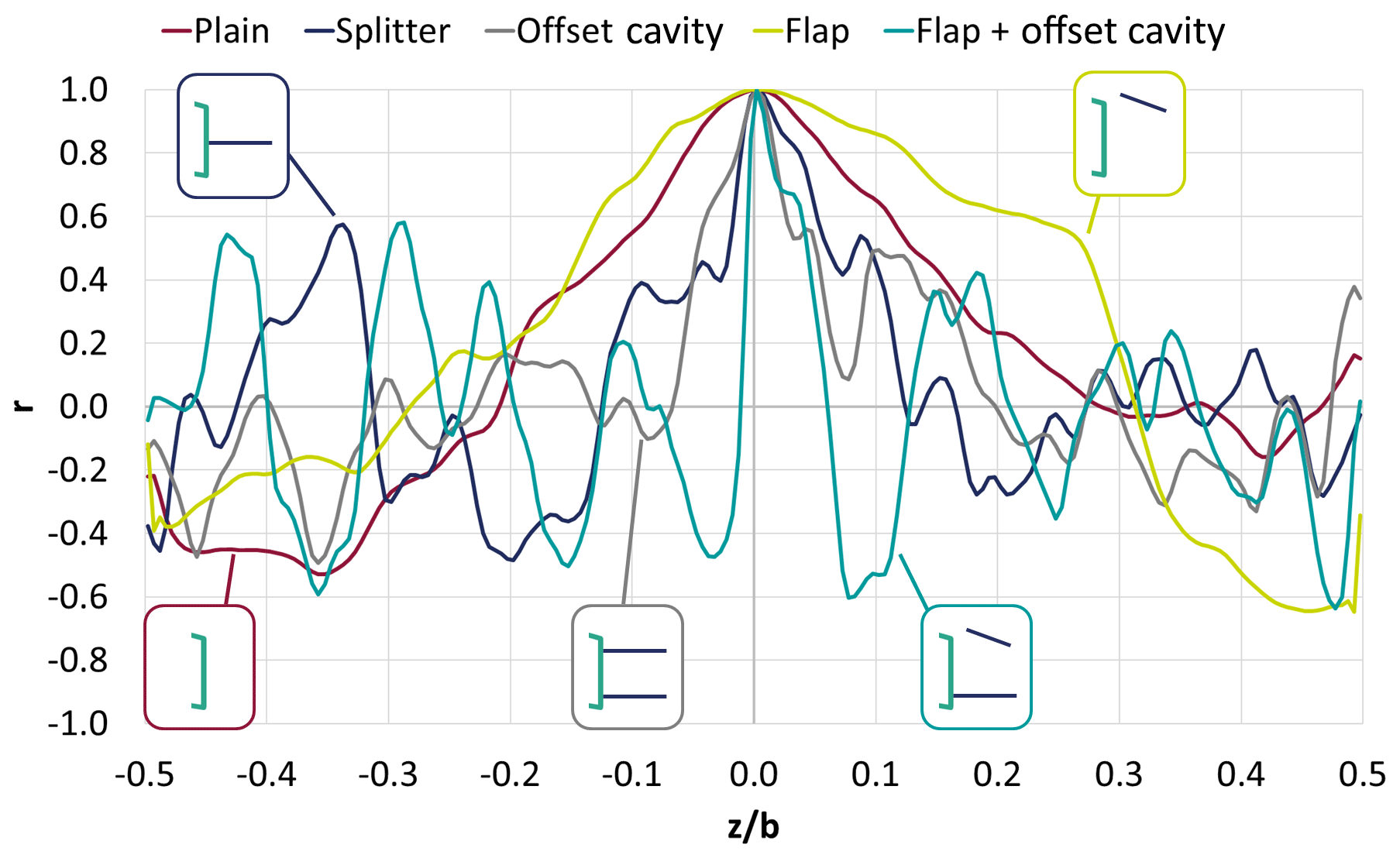
Figure 15Pearson correlation coefficient of the lift coefficient (Cl) time series with respect with the midsection (placed at ) for the various configurations. High positive values indicate strong positive correlation, and highly negative values suggest a strong negative correlation.
In order to quantify the spanwise correlation of the flow for each device, the Pearson correlation coefficient (r) of the Cl time signal at different spanwise locations is presented in Fig. 15. Values of 1 or −1 indicate strong correlation between the signals (positive and negative, respectively), while a value of 0 suggests no correlation. The correlation coefficient is calculated with respect to the midsection (located at in Fig. 15). It is evident that the TE devices significantly alter the spanwise correlation of the flow. When the plain configuration is examined, a correlation length of λ=0.5b, where b is the wing span, or λ=5hTE is identified, in agreement with Metzinger et al. (2018). For the flap case, the correlation length remains large with λ=5.9hTE. It is noted that in the flap case the lower vortex is shed-uncontrolled and this could explain the strong coherence in the wake. The splitter and offset cavity cases have the correlation length drop to λ=2.5hTE and λ=2.7hTE, respectively. The weakest spanwise coherence is observed for the flap + offset cavity case with λ=0.7hTE. The preceding analysis is also in agreement with the isosurfaces shown in Fig. 14. Indeed, as the figure suggests, the spanwise correlation length of the vorticity isosurfaces in the flap and offset cavity configuration is much smaller when compared to the flap configuration. Finally, it is noted here that using the wake velocity fluctuations for the preceding analysis yields similar results, however, the Cl was employed since it was already available at all spanwise stations.
3.3 Vortex formation
In the following, the mechanics of vortex shedding from the blunt TE, with and without the TE devices, are described. This analysis is only concerned with the spanwise vortices and their shedding from the wing TE or the devices TE. Naturally, this is a highly three-dimensional flow, and any description dealing only with spanwise-concentrated vortices is bound to be incomplete. Still, the spanwise vortex shedding mechanism is the one that dominates the wake flow and is also the one that subsequently gives rise to the three-dimensional features. Further, it is the modification of this mechanism, i.e. the modification of the roll up of the two shear layers into discrete vortices, that leads to the load changes for the airfoil and different St numbers in the wake. In this sense, it is considered of high importance to describe the flow in the airfoil wake. The description is based on the most accurate predictions, IDDES on a fine mesh, which are in good agreement with the experimental results.
Figures 16 to 20 present instantaneous isosurfaces of the Q criterion (Hunt et al., 1988) of all the examined cases. The shedding period (T) for each case has been split into six parts, and seven snapshots are shown. The isosurfaces are not coloured by any other quantity to avoid confusion, given the complexity of the structures. Red arrows indicate the location of the main spanwise vortices, as interpreted from the analysis of the results. It is highlighted that the analysis was supported by flow animations (Papadakis and Manolesos, 2020a, b), which cannot be included in the present document but were fundamental in understanding the flow mechanisms. It is noted that in order to offer the reader a broader view of the results, a different vortex identification criterion was selected in this case, compared to, e.g. Fig. 13. The selection of the criterion does not affect the conclusions of the study.
Starting with the plain airfoil case (Fig. 15) and following the descriptions of Gerrard (1966), Tombazis and Bearman (1997), and Williamson (1996), it is observed that the top vortex is fed with vorticity from the airfoil top boundary layer and grows in size and strength. During this period the vortex remains attached to the top side of the blunt trailing edge until eventually growing strong enough to draw the opposing shear across the wake. Following this, opposite-sign vorticity is entrained between the top shear layer and the top vortex, which is when the feeding of vorticity cedes and the vortex is shed in the wake. In a similar manner, the lower spanwise vortex is fed with vorticity from the airfoil lower boundary layer and is cut off when it draws a vorticity of opposite sign between itself and the feeding shear layer.
This “feeding” mechanism is present in all cases, but the presence of the flow control devices alters when and where the vortex is shed in the wake. In the splitter case (Fig. 16) it appears that there is constantly a vortical structure at both edges of the blunt TE. In an alternating manner these structures grow and shed a vortex across the splitter plate. It is noted that when the vortices leave the wing TE, they are much smaller in size and strength compared to the plain airfoil case. Furthermore, these vortices are not immediately shed in the wake but grow further at each side of the splitter plate, feeding from the adjacent shear layer (top or bottom) before they are eventually convected downstream. This mechanism has a higher frequency than the plain airfoil case (see also Fig. 7) and explains the longer formation length and smaller wake thickness observed in the experiments and simulations (see also Fig. 9).
In the offset cavity case (Fig. 17) the top vortex begins to form when the lower one is about to be shed into the wake. In that instant, they are both at the edges of the cavity plates. Following this, the top vortex grows, feeding from the top shear layer, while there is also a stationary vortical structure adjacent to the wing TE, between the top cavity plate and the wing TE. A similar structure exists at the bottom edge, between the wing and the lower plate. This structure is not stationary. As the top vortex grows, the lower structure is fed from the wing lower boundary layer and is elongated under the cavity lower plate. When the top vortex grows strong enough to be shed in the wake, the lower elongated vortical structure is split into the lower vortex and a vortical structure, remaining close to the wing lower TE. The lower vortex will shortly stand at the lower plate TE, before also being shed. The different behaviour of the vortical upper and lower structures is due to the different flow direction as it leaves the airfoil upper and lower sides and is directed into the wake and on the cavity plates. In the top side, the flow is directed towards the plate, while in the lower side it is directed away from it.
Figure 18 presents the flap + offset cavity case. The mechanics are similar to the offset cavity case, with two notable differences. Firstly, the top vortex now forms in at the TE edge of the flap, connected to its boundary layer, and secondly the lower elongated vortical structure is split after the top vortex is shed in the wake. The wake in general appears regular and considerably better structured compared to all the other cases. The flap changes the symmetrical wake pattern and reduces the St number with regards to the offset cavity case.
Finally, Fig. 19 shows the vortical structures for the flap case. Here, the top vortex is located at the TE of the flap and begins to form when the lower vortex, already shed from the lower TE of the wing, passes below it. The top vortex then remains almost stationary, growing in strength and size before it is eventually shed in the wake. In the meantime, a new lower vortex has been formed at the lower TE of the wing. The new vortex feeds from the wing lower boundary layer and is shed in the wake only after the top vortex has been convected. The lower vortex then travels under the flap, generating the top vortex as it passes below the flap TE. The wake is markedly more turbulent and less well-structured than the flap + offset cavity case. It is conceivable that this is because the lower vortex is stronger and more three-dimensional than in the flap + offset cavity case, where its formation was affected by the presence of the lower cavity plate.
A computational investigation of the flow past a flatback airfoil with and without TE control devices has been presented, and the results have been compared with wind tunnel measurements. Both URANS and IDDES modelling have been considered on two grids of different density, a coarse grid with 5 million cells and a fine grid with 25 million cells. Computations are compared with measurements in terms of forces, wake frequencies and stereo PIV measurements. Overall, if wake structure and frequencies are of interest, then the highest-fidelity simulation, IDDES on a fine mesh, should be preferred, as it provides the best agreement with experimental data in all cases and parameters. If, on the other hand, only the effect of the TE devices on the forces is of interest, then even the 2D URANS simulations can provide acceptable results. The simplest computational method, in agreement with the experiments and all other numerical predictions, suggests that the flap device outperforms all other examined flow control solutions in terms of lift and the lift-to-drag ratio.
In more detail, 2D URANS predictions give a qualitatively correct estimation of the TE device's relative performance. The load variation for the plain airfoil case, however, appears overestimated. There is fair comparison between the 3D URANS simulations and the experimental data in terms of forces and flow quantities for the plain airfoil case, especially on the fine mesh. For the cases with the TE devices, the 3D URANS forces predictions are in agreement with the measurements in terms of mean values, however, vorticity shedding is under-predicted or completely absent from the simulations. This is evident in the predicted St number being close to zero for the flap, cavity, and flap + offset cavity configurations. It is noted that increasing the mesh size from 5 to 25 million cells leads to similar results and no vorticity shedding.
On the contrary, IDDES simulations are in better agreement with the experimental data for all cases. The agreement is fair for both the unsteady characteristics and the predicted forces. IDDES modelling captures the unsteady character of the wake on both grids. Forces, however, appear to be unsteady only on the fine grid case on most cases. Naturally, refining the grid leads to a better comparison with the experimental data especially when comparing to stereo PIV measurements and St numbers.
Finally, using the most accurate predictions, IDDES on the fine mesh, the effect of the TE devices on the vortex formation and shedding has been analysed. In the plain airfoil case, the growth of the vortices as they receive vorticity from the airfoil boundary layers is apparent, followed by the shedding of the vortices in the wake in an alternating manner. All TE devices affect the shedding mechanism. In the splitter case, the vortices are formed on the airfoil upper and lower TE, and they are smaller in size compared to the plain airfoil case wherein they are shed in the wake. In the offset cavity case, the top vortex forms at the TE of the upper cavity plate, while the lower comes off an elongated vortical structure between the lower cavity plate and the airfoil TE. In the flap case, the top vortex forms at the TE of the flap and is fed by its boundary layer. In the flap + offset cavity case, the wake is better structured and less three-dimensional than all other cases, with the top vortex forming at the TE of the flap and the lower vortex splitting off the lower elongated vortical structure, as in the offset cavity case.
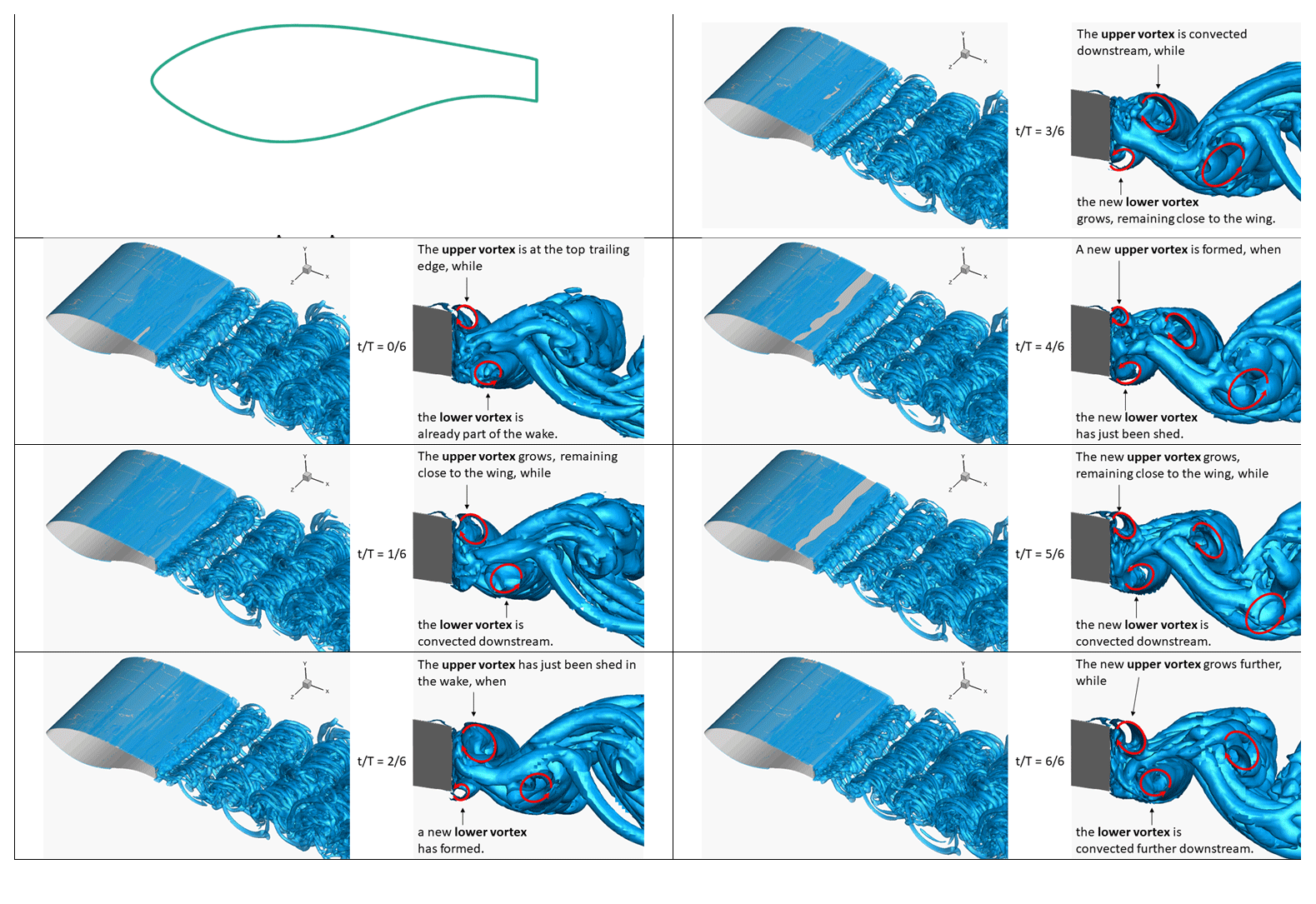
Figure A1Snapshots of Q isosurfaces from the plain airfoil case: IDDES fine-mesh results. Each period of the vortex shedding mechanism is split into six parts, and a total of seven snapshots is shown. For each snapshot, two visualisations are shown. A 3D view of Q=1.5 isosurfaces is shown on the left, and a side view of Q=100 isosurfaces is shown on the right. Superimposed red arrows indicate interpreted spanwise vortices.
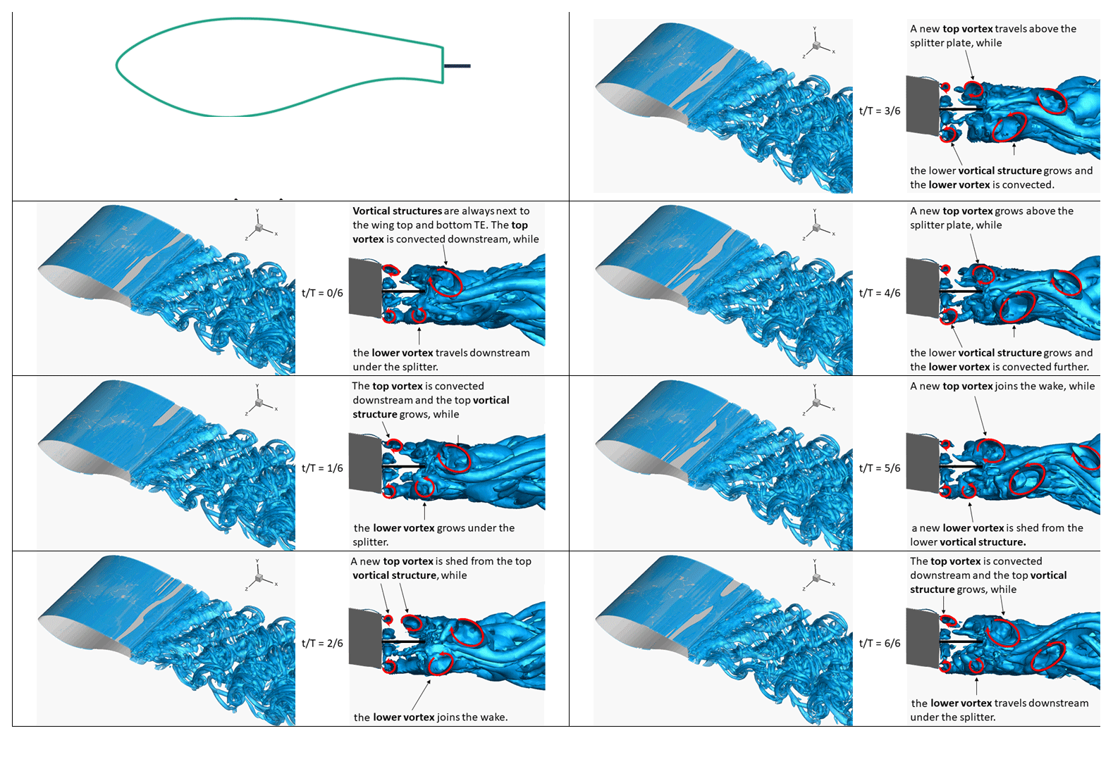
Figure A2Snapshots of Q isosurfaces from the splitter case: IDDES fine-mesh results. Each period of the vortex shedding mechanism is split into six parts, and a total of seven snapshots is shown. For each snapshot, two visualisations are shown.A 3D view of Q=1.5 isosurfaces is shown on the left, and a side view of Q=100 isosurfaces is shown on the right. Superimposed red arrows indicate interpreted spanwise vortices.
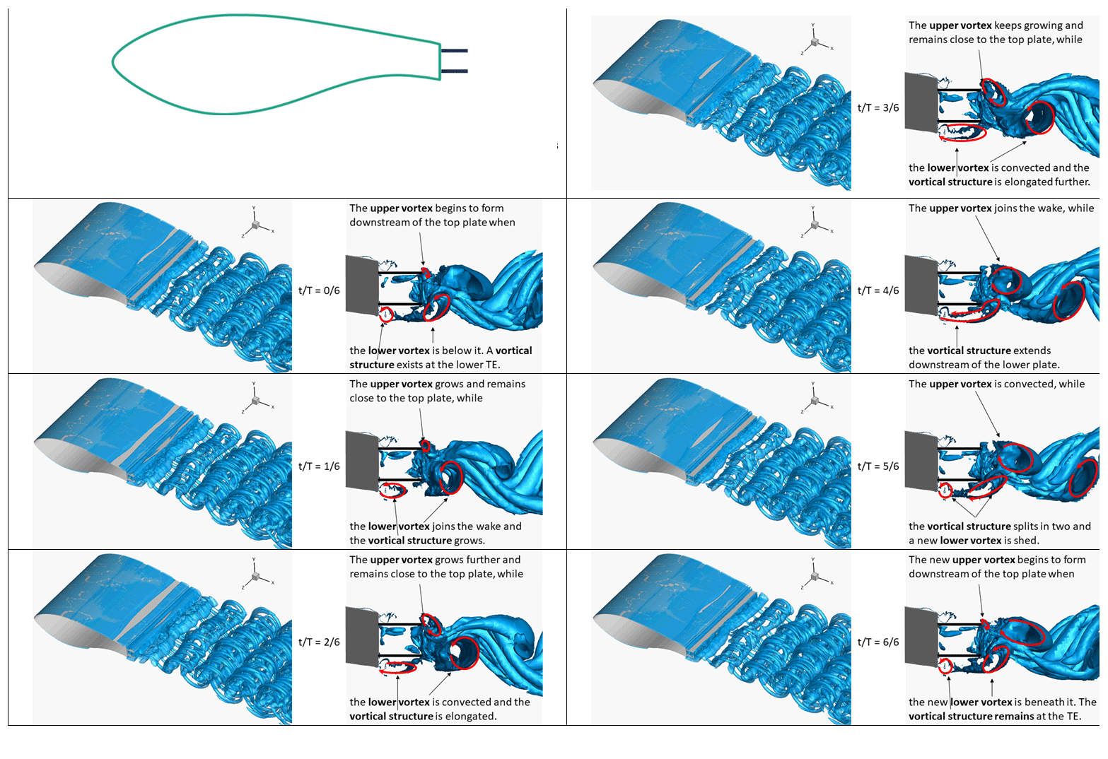
Figure A3Snapshots of Q isosurfaces from the offset cavity case: IDDES fine-mesh results. Each period of the vortex shedding mechanism is split into six parts, and a total of seven snapshots is shown. For each snapshot, two visualisations are shown. A 3D view of Q=1.5 isosurfaces is shown on the left, and a side view of Q=100 isosurfaces is shown on the right. Superimposed red arrows indicate interpreted spanwise vortices.
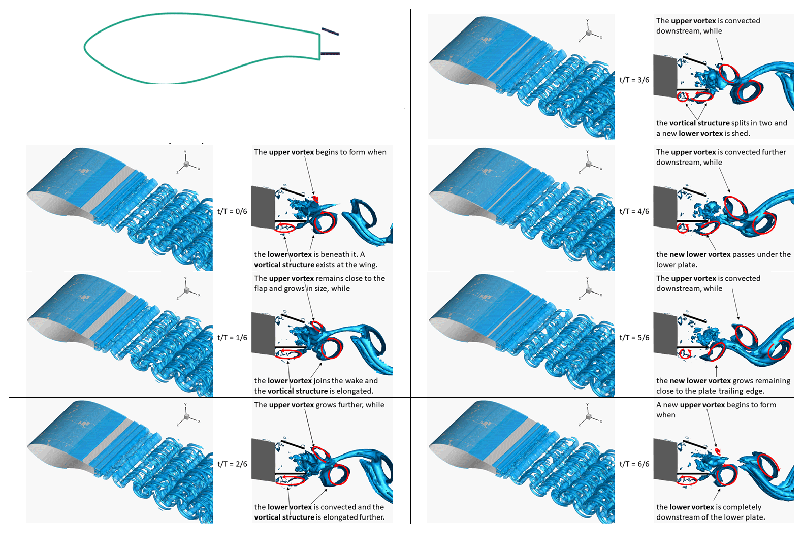
Figure A4Snapshots of Q isosurfaces from the flap + offset case: IDDES fine-mesh results. Each period of the vortex shedding mechanism is split into six parts, and a total of seven snapshots is shown. For each snapshot, two visualisations are shown. A 3D view of Q=1.5 isosurfaces is shown on the left, and a side view of Q=100 isosurfaces is shown on the right. Superimposed red arrows indicate interpreted spanwise vortices.
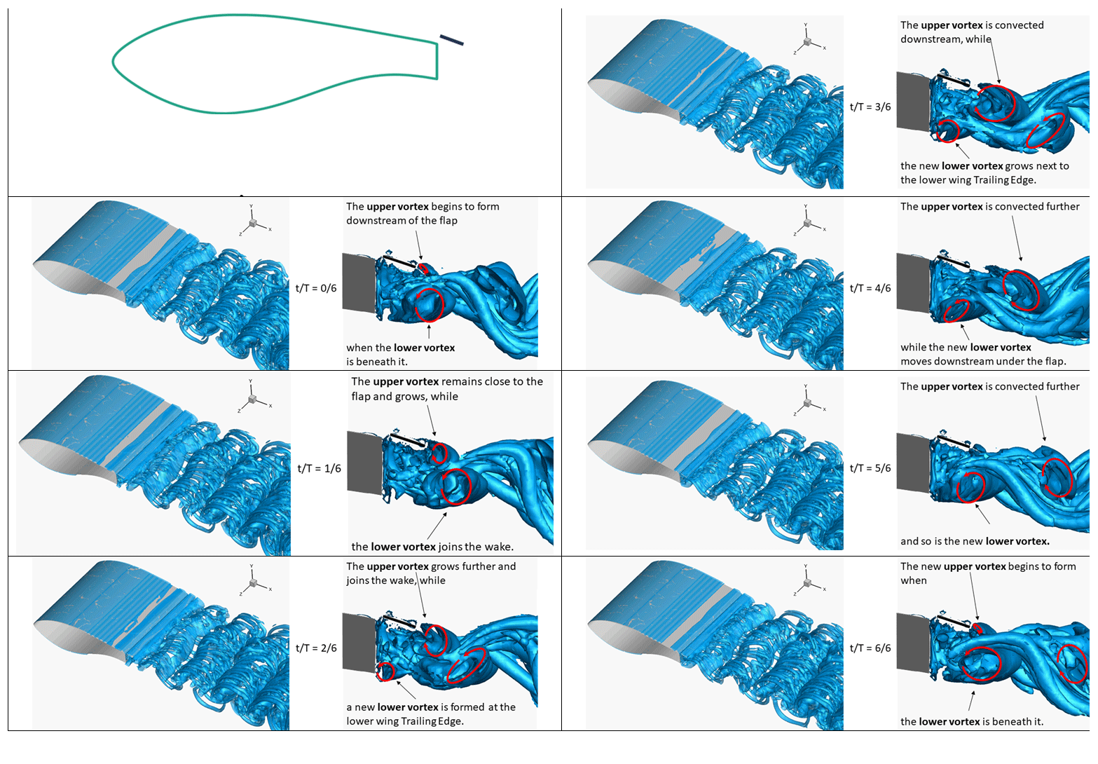
Figure A5Snapshots of Q isosurfaces from the flap case: IDDES fine-mesh results. Each period of the vortex shedding mechanism is split in six parts and a total of 7 snapshots is shown. For each snapshot, two visualisations are shown. A 3D view of Q=1.5 isosurfaces is shown on the left, and a side view of Q=100 isosurfaces is shown on the right. Superimposed red arrows indicate interpreted spanwise vortices.
Table A1Mean and standard deviation (σ) values for lift and drag coefficients. Comparison between experiments and IDDES results for the coarse and fine mesh.
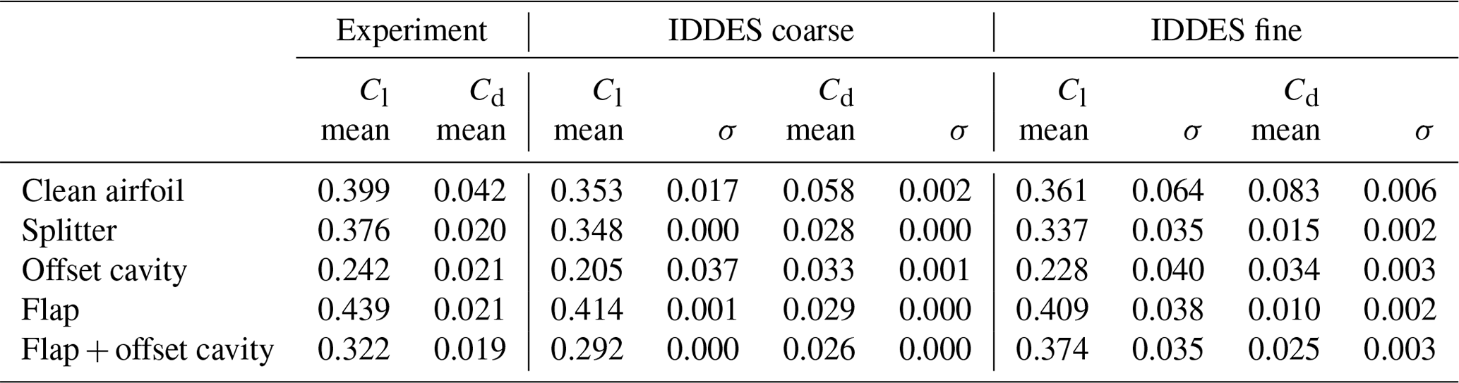
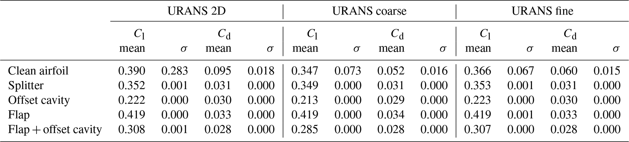
Table A2Mean and standard deviation (σ) values for lift and drag coefficients. Comparison between 2D URANS and URANS on the coarse and fine mesh.
Code is available upon request.
All data are available upon request.
GP performed the numerical calculations. For the analysis and investigations of the numerical and experimental results the contribution of the authors was equal. Both authors contributed equally to manuscript authorship.
The authors declare that they have no conflict of interest.
This article is part of the special issue “Wind Energy Science Conference 2019”. It is a result of the Wind Energy Science Conference 2019, Cork, Ireland, 17–20 June 2019.
Computational resources were provided by HPC Wales, which is gratefully acknowledged.
Marinos Manolesos would like to acknowledge the contribution of the Supergen Early Career Researcher Fund Award from the Supergen Offshore Renewable Energy Hub, EPSRC.
This research has been supported by the Supergen Offshore Renewable Energy Hub, EPSRC, through the Supergen Early Career Researcher Fund Award.
This paper was edited by Julie Lundquist and reviewed by two anonymous referees.
Bai, H. and Alam, M. M.: Dependence of square cylinder wake on Reynolds number, Phys. Fluids, 30, 015102, https://doi.org/10.1063/1.4996945, 2018.
Baker, J. P. and Van Dam, C. P.: Drag reduction of a blunt trailing-edge airfoil, University of California, Davis, 20–24, 2009.
Baker, J. P., Mayda, E. A., and Van Dam, C. P.: Experimental analysis of thick blunt trailing-edge wind turbine airfoils, J. Sol. Energ.-T. Asme., 128, 422–431, 2006.
Barone, M. F. and Berg, D.: Aerodynamic and aeroacoustic properties of a flatback airfoil: an update, 2009 – 271, in: 47th AIAA Aerospace Sciences Meeting Including The New Horizons Forum and Aerospace Exposition, Orlando, Florida, https://doi.org/10.2514/6.2009-271, 2009.
Boorsma, K., Muñoz, A., Méndez, B., Gómez, S., Irisarri, A., Munduate, X., Sieros, G., Chaviaropoulos, P., Voutsinas, S. G., Prospathopoulos, J., Manolesos, M., Shen, W. Z., Zhu, W., and Madsen, H.: New airfoils for high rotational speed wind turbines, INNWIND.EU D2.12 Deliverable, available at: http://www.innwind.eu/-/media/Sites/innwind/Publications/Deliverables/Deliverable-2-12_hama_10-09-2015_final.ashx?la=da&hash=21B731CDDEAD9D4F8A027A22553A79FA1A16C50C (last access: 31 January 2020), 2015.
Calafell, J., Lehmkuhl, O., Rodriguez, I., and Oliva, A.: On the Large-Eddy Simulation modelling of wind turbine dedicated airfoils at high Reynolds numbers, ICHMT Digit. Libr. ONLINE 2012-September, 1419–1430, 2012.
Choi, H., Jeon, W.-P., and Kim, J.: Control of flow over a bluff body, Annu. Rev. Fluid Mech., 40, 113–139, 2008.
Chong, M. S., Perry, A. E., and Cantwell, B. J.: A general classification of three-dimensional flow fields, Phys. Fluids A, 2, 765–777, https://doi.org/10.1063/1.857730, 1990.
Gerrard, J. H.: The mechanics of the formation region of vortices behind bluff bodies, J. Fluid Mech., 25, 401–413, https://doi.org/10.1017/S0022112066001721, 1966.
Griffith, D. T. and Richards, P. W.: The snl100-03 blade: Design studies with flatback airfoils for the sandia 100-meter blade, SANDIA Report, SAND2014-18129, 2014.
Hossain, M. M., Stoevesandt, B., and Peinke, J.: Higher Order DNS on an Airfoil Fx77-W500 Using Spectral/hp Method, Glob. J. Sci. Front. Res., 13, 2013.
Hunt, J. C. R., Wray, A. A., and Moin, P.: Eddies, streams, and convergence zones in turbulent flows, in: Studying Turbulence Using Numerical Simulation Databases, 2, 193–208, 1988.
Kahn, D. L., van Dam, C. P., and Berg, D. E.: Trailing edge modifications for flatback airfoils, SANDIA Report, SAND2008-1781, Sandia National Laboratories, 2008.
Kim, T., Jeon, M., Lee, S., and Shin, H.: Numerical simulation of flatback airfoil aerodynamic noise, Renew. Energ., 65, 192–201, https://doi.org/10.1016/j.renene.2013.08.036, 2014.
Krentel, D. and Nitsche, W.: Investigation of the near and far wake of a bluff airfoil model with trailing edge modifications using time-resolved particle image velocimetry, Exp. Fluids, 54, 1551, https://doi.org/10.1007/s00348-013-1551-1, 2013.
Lehmkuhl, O., Calafell, J., Rodríguez, I., and Oliva, A.: Large-Eddy Simulations of Wind Turbine Dedicated Airfoils at High Reynolds Numbers, in: Wind Energy-Impact of Turbulence, edited by: Hölling, M., Peinke, J., and Ivanell, S., Springer, Berlin, Heidelberg, 147–152, https://doi.org/10.1007/978-3-642-54696-9_22, 2014.
Manolesos, M., Papadakis, G., and Voutsinas, S.: An experimental and numerical investigation on the formation of stall-cells on airfoils, J. Phys. Conf. Ser., 555, 012068, https://doi.org/10.1088/1742-6596/555/1/012068, 2014a.
Manolesos, M., Papadakis, G., and Voutsinas, S. G.: Assessment of the CFD capabilities to predict aerodynamic flows in presence of VG arrays, J. Phys. Conf. Ser., 524, 012029, https://doi.org/10.1088/1742-6596/524/1/012029m, 2014b.
Manolesos, M., Papadakis, G., and Voutsinas, S. G.: Experimental and computational analysis of stall cells on rectangular wings, Wind Energy, 17, 939–955, https://doi.org/10.1002/we.1609, 2014c.
Manolesos, M., Papadakis, G., and Voutsinas, S.: Study of Drag Reduction Devices on a Flatback Airfoil, in: 34th Wind Energy Symposium, American Institute of Aeronautics and Astronautics, Reston, Virginia, https://doi.org/10.2514/6.2016-0517, 2016a.
Manolesos, M. and Voutsinas, S. G.: Experimental Study of Drag-Reduction Devices on a Flatback Airfoil, AIAA J., 54, 3382–3396, https://doi.org/10.2514/1.J054901, 2016b.
Mayda, E. A., van Dam, C. P., Chao, D. D., Berg, D. E., Baker, J. P., van Dam, C. P., and Gilbert, B. L.: Flatback airfoil wind tunnel experiment, Sandia Report, SAND2008-2008, Sandia National Laboratories, Albuquerque, NM, USA, 2008.
Menter, F.: Zonal two equation kw turbulence models for aerodynamic flows, in: 23rd fluid dynamics, plasmadynamics, and lasers conference, p. 2906, 1993.
Metzinger, C. N., Chow, R., Baker, J. P., Cooperman, A. M., and van Dam, C. P.: Experimental and Computational Investigation of Blunt Trailing-Edge Airfoils with Splitter Plates, AIAA J., 56, 3229–3239, https://doi.org/10.2514/1.J056098, 2018.
Mittal, R. and Balachandar, S.: Generation of streamwise vortical structures in bluff body wakes, Phys. Rev. Lett., 75, 1300–1303, https://doi.org/10.1103/PhysRevLett.75.1300, 1995.
Nash, J. F.: A discussion of two-dimensional turbulent base flows, Reports and Memoranda No. 3468, Aeronautical Research Council, London, 1965.
Papadakis, G. and Manolesos, M.: The flow past a flatback airfoil with flow control devices: Benchmarking numerical simulations against wind tunnel data – Animations, Zenodo, https://doi.org/10.5281/ZENODO.3662124, 2020a.
Papadakis, G. and Manolesos, M.: The flow past a flatback airfoil with flow control devices: Benchmarking numerical simulations against wind tunnel data – Animations II, Zenodo, https://doi.org/10.5281/ZENODO.3876198, 2020b.
Papadakis, G. and Voutsinas, S. G.: A strongly coupled Eulerian Lagrangian method verified in 2D external compressible flows, Comput. Fluids, 195, 104325, https://doi.org/10.1016/j.compfluid.2019.104325, 2019.
Shur, M. L., Spalart, P. R., Strelets, M. K., and Travin, A. K.: A hybrid RANS-LES approach with delayed-DES and wall-modelled LES capabilities, Int. J. Heat. Fluid Fl., 29, 1638–1649, https://doi.org/10.1016/j.ijheatfluidflow.2008.07.001, 2008.
Sørensen, N. N., Méndez, B., Muñoz, A., Sieros, G., Jost, E., Lutz, T., Papadakis, G., Voutsinas, S., Barakos, G. N., Colonia, S., Baldacchino, D., Baptista, C., and Ferreira, C.: CFD code comparison for 2D airfoil flows, Journal of Physics: Conference Series, Institute of Physics Publishing, https://doi.org/10.1088/1742-6596/753/8/082019, 2016.
Spalart, P. and Allmaras, S.: A one-equation turbulence model for aerodynamic flows, in: 30th Aerospace Sciences Meeting and Exhibit. American Institute of Aeronautics and Astronautics, Reno, NV, 5–21, https://doi.org/10.2514/6.1992-439, 1992.
Standish, K. J. and Van Dam, C. P.: Aerodynamic analysis of blunt trailing edge airfoils, J. Sol. Energ.-T. Asme, 125, 479–487, 2003.
Stone, C., Tebo, S., and Duque, E. P. N.: Computational Fluid Dynamics of Flatback Airfoils for Wind Turbine Applications, in: 44th AIAA Aerospace Sciences Meeting and Exhibit, American Institute of Aeronautics and Astronautics, Reston, Virigina, https://doi.org/10.2514/6.2006-194, 2006.
Stone, C., Barone, M., Smith, M., and Lynch, E.: A Computational Study of the Aerodynamics and Aeroacoustics of a Flatback Airfoil Using Hybrid RANS-LES, in: 47th AIAA Aerospace Sciences Meeting Including The New Horizons Forum and Aerospace Exposition. American Institute of Aeronautics and Astronautics, Reston, Virigina, https://doi.org/10.2514/6.2009-273, 2009.
Tanner, M.: Reduction of base drag, Prog. Aerosp. Sci., 16, 369–384, 1975.
Tombazis, N. and Bearman, P. W.: A study of three-dimensional aspects of vortex shedding from a bluff body with a mild geometric disturbance, J. Fluid Mech., 330, 85–112, https://doi.org/10.1017/S0022112096003631, 1997.
Viswanath, P. R.: Flow management techniques for base and afterbody drag reduction, Prog. Aerosp. Sci., 32, 79–129, 1996.
Williamson, C. H. K.: Vortex dynamics in the cylinder wake, Annu. Rev. Fluid Mech., 28, 477–539, https://doi.org/10.1146/annurev.fl.28.010196.002401, 1996.
Xu, H., Shen, W., Zhu, W., Yang, H., and Liu, C.: Aerodynamic Analysis of Trailing Edge Enlarged Wind Turbine Airfoils, Journal of Physics: Conference Series, IOP Publishing, p. 12010, 2014.