the Creative Commons Attribution 4.0 License.
the Creative Commons Attribution 4.0 License.
 | 06 Aug 2020
Validation of uncertainty reduction by using multiple transfer locations for WRF–CFD coupling in numerical wind energy assessments
Rolf-Erik Keck
Niklas Sondell
This paper describes a method for reducing the uncertainty associated with utilizing fully numerical models for wind resource assessment in the early stages of project development. The presented method is based on a combination of numerical weather predictions (NWPs) and microscale downscaling using computational fluid dynamics (CFD) to predict the local wind resource. Numerical modelling is (at least) 2 orders of magnitude less expensive and time consuming compared to conventional measurements. As a consequence, using numerical methods could enable a wind project developer to evaluate a larger number of potential sites before making an investment. This would likely increase the chances of finding the best available projects.
A technique is described, multiple transfer location analysis (MTLA), where several different locations for performing the data transfer between the NWP and the CFD model are evaluated. Independent CFD analyses are conducted for each evaluated data transfer location. As a result, MTLA will generate multiple independent observations of the data transfer between the NWP and the CFD model. This results in a reduced uncertainty in the data transfer, but more importantly MTLA will identify locations where the result of the data transfer deviates from the neighbouring locations. This will enable further investigation of the outliers and give the analyst a possibility to correct erroneous predictions. The second part is found to reduce the number and magnitude of large deviations in the numerical predictions relative to the reference measurements.
The Modern Energy Wind Assessment Model (ME-WAM) with and without MTLA is validated against field measurements. The validation sample for ME-WAM without MTLA consists of 35 observations and gives a mean bias of −0.10 m s−1 and a SD of 0.44 m s−1. ME-WAM with MTLA is validated against a sample of 45 observations, and the mean bias is found to be +0.05 m s−1 with a SD of 0.26 m s−1. After adjusting for the composition of the two samples with regards to the number of sites in complex terrain, the reduction in variability achieved by MTLA is quantified to 11 % of the SD for non-complex sites and 35 % for complex sites.
- Article
(3427 KB) - Full-text XML
- BibTeX
- EndNote


In the early stages of wind project development, it is common to consider a large number of potential sites. The majority of these potential sites typically do not contain an on-site measurement of climatic conditions. As on-site measurements are both expensive and time consuming, there is a practical limit to the number of sites that a developer can investigate using conventional methods. As a consequence, the number of potential sites considered is reduced at an early stage. This step may reduce the number of sites considered by an order of magnitude (e.g. from approximately 100 down to 10) to achieve a manageable portfolio for further analysis. As these decisions are often taken with limited data available, there is the risk of discarding some of the best projects in the process.
A remedy to mitigate the risk of advancing an suboptimal subset of sites for further analysis is to use high-quality numerical methods. As numerical methods are (at least) 2 orders of magnitude less time consuming and expensive compared to conventional on-site measurements used for early project selection, such as sodar or lidar measurements, it allows developers to evaluate a much larger set of projects. As an example, the numerical method presented in this work can be used to investigate on the order of 100 projects spread out over an area the size of Sweden in a time frame of 10 weeks for the cost of a single measurement campaign. However, on crucial aspect for the feasibility of such methods is the resulting uncertainty in the wind resource estimate. If the uncertainty is too high, compared to the real difference in wind resource between the investigated projects, the developer may reach the wrong conclusions.
As a result of this large potential, the field of numerical wind resource assessment is a mature research topic and there are a multitude of different approaches investigated. The most relevant work in relation to this paper are the methods based on numerical weather prediction (NWP) using the Wind Research and Forecast (WRF) model (Skamarock et al. 2008). WRF can be used to produce sufficiently accurate local wind speed estimates for early-stage wind resource assessments in flat terrain and for offshore applications (Draxl et al., 2015; Hahmann et al., 2015; Mylonas-Dirdiris et al., 2016; Ohsawa et al., 2016; Standen et al., 2017). However, it has also been observed that the prediction error and uncertainty in local wind speed estimates using WRF are correlated with increasing terrain complexity (Flores-Maradiaga et al., 2019; Giannaros et al., 2017; Prósper et al., 2019). To increase the accuracy in moderate and complex terrain, higher-resolution models are desirable to resolve the microscale effects. With respect to conducting wind energy assessments in the early stage of project development, the increased resolution also improves the ability to quantify the spatial extent of the areas with favourable wind conditions, i.e. the size of the potential wind farm, as well as allows the developer to better identify suitable terrain formations and other areas with relatively small characteristic length scales. Mortensen et al. (2017) discuss a combination of WRF and WAsP (WAsP, 1987) to include the effect of microscale terrain. Standen et al. (2017) describe a linearized microscale correction in their virtual met-mast approach. The microscale effects have also been modelled by coupling WRF with a large variety of non-linear computational fluid dynamics (CFD) models (e.g. Gopalan et al., 2014; Haupt et al., 2019; Quon et al., 2019).
The work presented here is based on the Modern Energy Wind Assessment Model (ME-WAM), which is a combination of WRF and a non-linear CFD model. The coupling to WRF is achieved through a virtual met mast, in which roughness- and terrain-corrected long-term-normalized time series from WRF is imported. The ME-WAM model was originally presented at the Wind Europe conference (Keck et al., 2019). In this paper we describe a method for reducing the uncertainty associated with utilizing NWP–CFD coupled via an internal forcing point for wind resource assessments. We have developed a technique, multiple transfer location analysis (MTLA), where several different locations for performing the data transfer between the NWP and the CFD model are evaluated. Independent CFD analyses are conducted for each evaluated data transfer location. As a result, MTLA will generate multiple independent observations of the data transfer between the NWP and the CFD model. This yields a reduced overall uncertainty, as well as a reduction in the number of large outliers in the distribution.
The Modern Energy Wind Assessment Model (ME-WAM) is a numerical model for assessing the feasibility of early-stage wind projects in absence of on-site wind measurements. The method is based on a combination of NWP in WRF and a steady-state non-linear CFD simulation to capture the microscale terrain. This allows for a fast and computationally effective method which retains the ability to capture mesoscale effects from WRF, as well as the capability to model local terrain, roughness, and forest effects at high resolution; see Fig. 1.
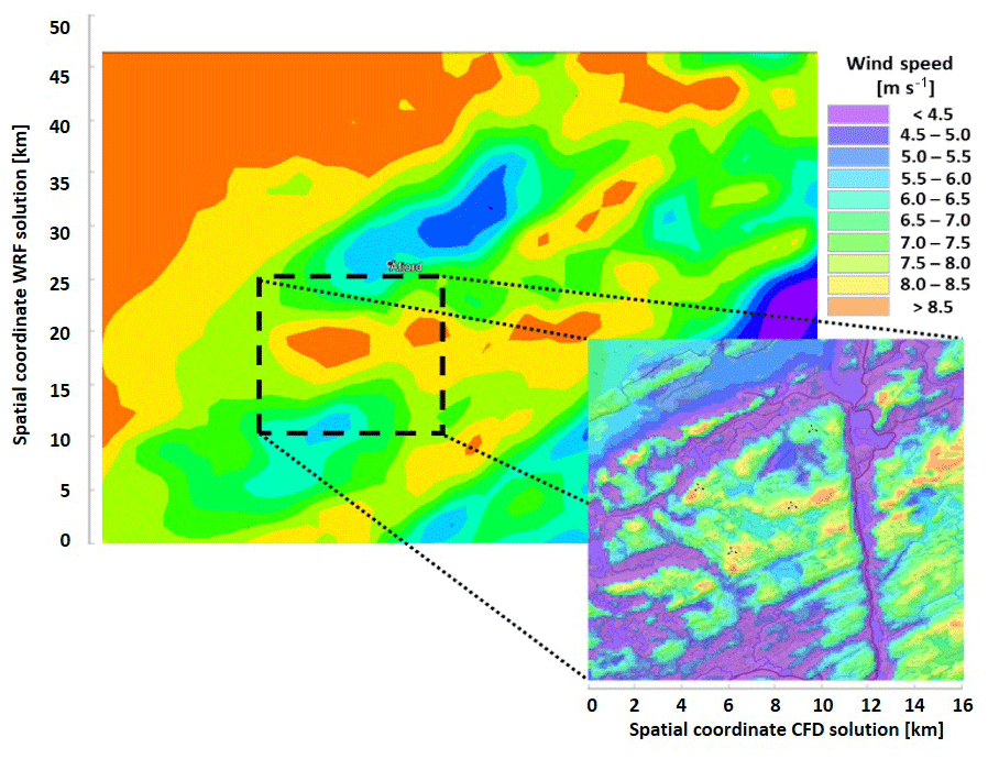
Figure 1Illustration of the ME-WAM method. The background contour is extracted mean wind speed from the WRF model. The black dashed box indicates the location where a microscale CFD analysis is conducted to add resolution in the results. By comparing the two velocity fields, which have the same colour setting, it is clear that the microscale effects are important to assess the local wind speed and to be able to design a wind farm in the investigated area.
The coupling between WRF and the CFD solver is achieved through a virtual met-mast approach. The WRF data are corrected based on regional roughness and terrain, as well as long-term normalized against the ERA5 reanalysis dataset (Copernicus Climate Change Service, 2017). The corrected time series is inserted into the CFD domain. This has the benefit of delivering a stable and straightforward coupling between the models. In the CFD model this is the same process as using a measured time series. A drawback, however, is that the virtual met-mast approach is sensitive to the location of the data transfer. It is crucial to find an appropriate location where the wind regime is sufficiently similar in the WRF and the CFD simulation to achieve good results.
Figure 2 displays an overview of the ME-WAM modelling process. The method only requires project coordinates as input and utilizes open data sources from WRF and other available GIS data to simulate the mesoscale wind regime. Modern Energy has developed a technique to optimize the data transfer location based on surrounding terrain, slopes, roughness, and expected mesoscale effects. We also apply a long-term normalization of the extracted WRF data. These steps occur in the “ME-WAM CORE” step. In the last step of the process, the information from the virtual met mast is applied in a CFD simulation to generate wind resource files, as well as turbulence and wind shear maps.
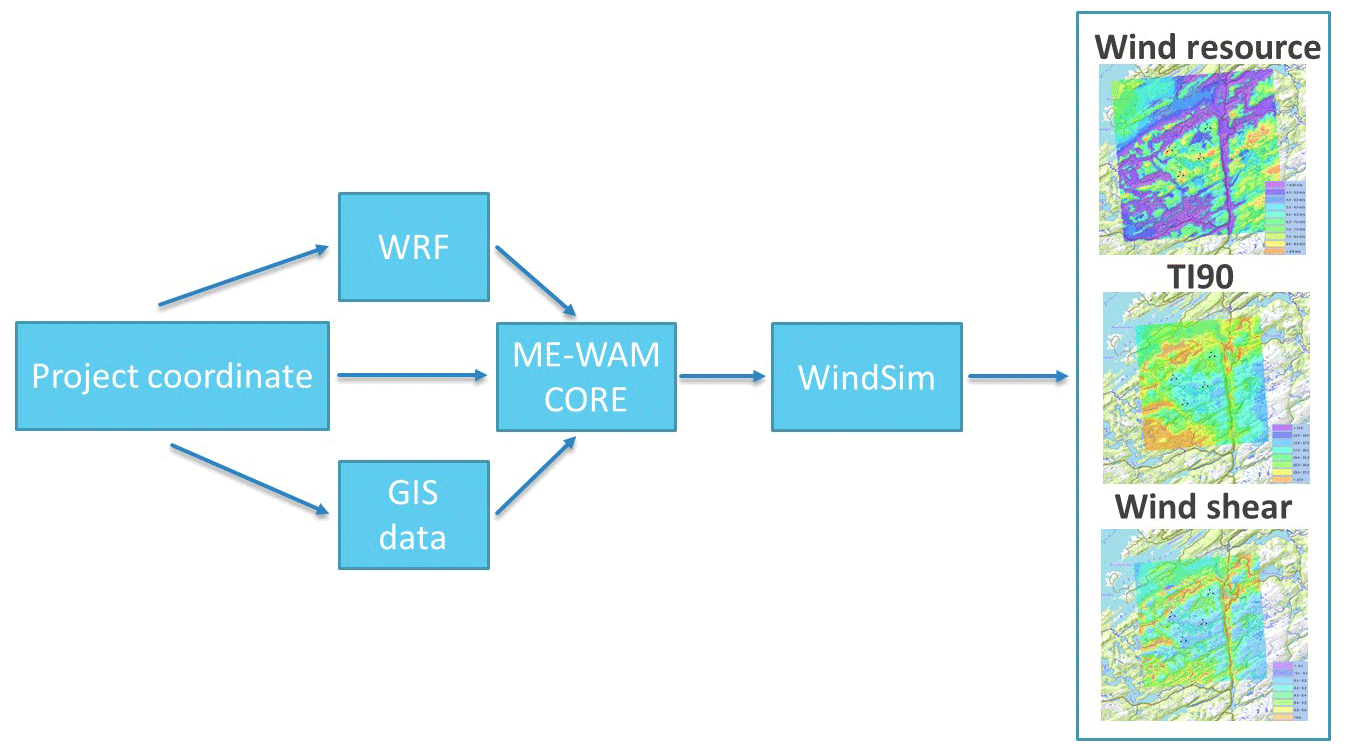
Figure 2Schematic description of the ME-WAM model process.
In the following sections the WRF and CFD model configurations used in our validation are briefly described. The algorithms for optimizing the data transfer location, as well as the corrections applied, and long-term normalization will not be described in further detail as they are proprietary information.
The large-scale wind regime at the simulated sites is predicted using numerical weather simulations conducted in the advanced research version of the Weather Research and Forecasting model (WRF-ARW) (Skamarock et al., 2008). The WRF model is an open-source state-of-the-art weather model which is widely used in both industry and the research environment. It is a comprehensive model which includes all relevant processes of heat, mass, and momentum transfer and thereby has the fidelity to be used for simulating a wide range of weather phenomena from large synoptic scales down to the meso- and even microscale.
The WRF-ARW model is based on the compressible nonhydrostatic Euler equations formulated using a terrain-following pressure level as the vertical coordinate. The model contains a large number of methods for parameterizations to handle land-surface properties, surface layer that governs near-surface turbulence fluxes, vertical transfer in the planetary boundary layer (PBL), short- and long-wave radiation budget, microphysics, and cumulus formation, for example. The appropriate selection of these schemes is dependent on both the numerical setup of the model (most noticeably the spatial resolution of the computational grid) and the most important physics for the investigated sites. Care must be taken when selecting the combinations of parameterizations as they interact with each other.
In this work the WRF configuration has been customized to the various sites based on internal best practice for the different locations and topographies investigated. The details of each case are not considered to be relevant for the research described here. There are some common configurations for all cases. The WRF simulations are conducted with the two-way nesting approach on three domains. The horizontal resolution of these domains was 13.5, 4.5, and 1.5 km. The vertical mesh contains 42 vertical levels, with fine meshing near the surface and vertical stretching in higher levels. In Europe the GMTED dataset with 500 m resolution was used as terrain representation and CORINE with 100 m spatial resolution was used as the input roughness. The ERA5 reanalysis dataset (Copernicus Climate Change Service, 2017) is used as initial and boundary conditions. The parameterizations vary based on regional verifications, but in general the more advanced options for the surface layer, PBL, and micro-physics are applied.
The microscale effects are incorporated by performing CFD downscaling of the mesoscale wind regime using the commercial CFD software package WindSim (from Vector AS); see Fig. 1. WindSim is based on the Phoenics solver (Phoenics flow solver, 2020) and solves the three-dimensional incompressible RANS (Reynolds-averaged Navier–Stokes) equations. The equations are solved on a Cartesian grid, and multiple grid refinement regions and grid stretching can be applied. The convective terms are discretized using the hybrid differencing scheme (i.e. a combination of the first-order upwind scheme and the second-order central differencing scheme), and the diffusion terms are discretized by the central differencing scheme. The pressure–velocity coupling is achieved using the SIMPLEST algorithm. There are multiple turbulence closures available in the solver. In this work the standard k−ε model (Launder and Sharma, 1974) has been used. WindSim has functionality to model the effect of atmospheric stability by including buoyancy effects using the Boussinesq approximation and by modifying the inlet boundary conditions and boundary layer height. WindSim also has functionality for modelling forest effects as distributed volume forces in the CFD domain.
For this application, where WindSim is used to downscale WRF data imposed as a virtual met mast, one must consider a balance between high representation of details in the flow field and small-scale phenomena (such as terrain-induced flow separation in the context) with the requirement for a smooth and predictable flow field which can be coupled to the large-scale dynamics represented by the WRF simulation. The imposed WRF time series will be scaled based on difference in flow conditions between any location in the CFD domain and that at the mast location to produce a wind resource map over the area. As a consequence, the transfer location between WRF and WindSim is important to achieve a stable and robust output for the ME-WAM modelling chain as any errors at the transfer location are propagated out to the whole wind resource map. In this work all WindSim simulations have been conducted using a central refinement region of equidistant Cartesian mesh with a horizontal resolution of 100 m in a 25 km by 25 km region. The mesh is stretched outwards from the equidistant region in the outer domain. The size and height of the outer domain vary based on local topography. The vertical mesh consists of 40 vertical cells. There are 10 cells within the first 80 m to resolve the boundary layer. The y+ value for the near-wall modelling is maintained at a value on the order of 50 (the wall model applied is valid in the range between 30 and 130 according to the Phoenics documentation). The vertical cell sizes then increase with height from the ground.
Steady-state simulations are conducted for 12 sectors of 30∘ each. The general collocated velocity (GCV) method was used for solving the governing equations and the standard k−ε model for turbulence closure. Forest is described by 18 classes based on height and tree type. The forest resistive value varies between 0.025 and 0.2 in the various classes.
As described above, the modelling chain in ME-WAM is based on a WRF simulation coupled to a CFD model via an internal forcing point. Experience has shown that the data transfer and downscaling between WRF and the CFD model are the link with the highest uncertainty in the ME-WAM method. The multiple transfer location analysis (MTLA) technique is based on conducting the data transfer and CFD downscaling through several different transfer locations, each with independent CFD simulations. As a result, MTLA will generate multiple independent realizations of the data transfer and the CFD downscaling. The hypothesis is that this will result in a reduced overall uncertainty in the modelling chain, but even more importantly it should result in a reduction in the number of large outliers in the distribution. A reduction of large outliers will be probable as the multiple predictions of mean wind speed at a single location will help identify results that deviate from the surrounding analyses. These transfer points and CFD simulations can thereafter be investigated further and root causes for the deviations can be identified and corrected for.

Figure 3Illustration of the MTLA method where the wind speed at the target location (grey marker) is predicted based on three separate ME-WAM analyses. The black markers indicate the data transfer locations. The colour scale in the background represents mean wind speed at 100 , red represents high wind, and blue represents low wind in a range from 5 to 8 m s−1.
The hypothesis above is formulated based on observations that ME-WAM is found to give consistent result across the extracted 25 km × 25 km result surfaces. At instances where multiple ME-WAM analyses have been conducted to predict the wind speed at a specific location, it has been found that as long as the ME-WAM core (see Fig. 2) has been able to identify a suitable location for WRF–CFD coupling, the difference in the predictions is generally small. This ability was also verified for seven wind farms with a total sample of over 300 wind turbines by Keck et al. (2019). As an example, consider the data in Fig. 3. Three different ME-WAM analyses have been conducted to predict the mean wind speed at the location of the grey marker. The transfer location between WRF and the CFD model is indicated by the black markers. The data transfer has been confirmed to occur at a suitable location for all three analyses. Even though the data transfers have occurred at distances varying from 3 to 20 km, all three analyses produce estimates within 1 % deviation of target mean wind speed in this case (7.06, 7.09, and 7.13 m s−1).
One aspect that is important to consider is that the two underlying models have different capabilities. The WRF model includes mesoscale effects which cannot be captured by the CFD model. As a consequence, care must be taken to consider any gradients in the velocity field caused by mesoscale effects (as discussed by Haupt et al., 2019). When mesoscale gradients are present in the simulated region, there should be a difference in the predictions of two independent CFD models. Examples of such effects to consider are land–sea interactions in coastal areas, capping inversions, or mesoscale stability effects in mountain areas.
In this work, four analyses have been made for each location were the MTLA method is utilized. The drawback of this approach is that the second half of the modelling chain becomes 4 times as computationally demanding due to the duplication of work. If a significant reduction in uncertainty can be achieved, however, this method has the potential to increase the applicability for numerical modelling for wind assessments. The added computational cost with the proposed simulation configuration is on the order of 500 CPU hours.
The validation data used in the work are obtained through collaborations with wind project developers. In total 11 developers have contributed data, and a total of 80 meteorological masts are available for the validation campaign. The available data represent a large variation in topographical conditions and geographical spread. The dataset is considered to cover the range of normal conditions experienced in wind project assessment, as it includes sites with severely complex terrain, coastal conditions, rolling hills, and varying degrees of forest coverage; see Fig. 4.

Figure 4The variations in terrain and roughness covered in the validation dataset. Panel (a) depicts a site in complex terrain on the Norwegian west coast and (b) a forested inland site in Sweden.
The evaluation of the ME-WAM model and the MTLA is based on a blind test in which the ME-WAM prediction is compared to the measured and long-term-corrected wind speed. In this process the collaborating company provides a project coordinate somewhere in the vicinity of the metrological mast. Modern Energy subsequently conducts a ME-WAM analysis and sends the resulting wind resource files to the collaborating company. The collaborating company finally compares the numerical results to their measured and long-term-corrected wind speed at the mast location.
A drawback of this validation method is that the field data are not available to the authors for quality control. However, as the measurements are conducted and analysed to be used for wind farm development, and are often scrutinized by a third party of the collaborating companies, the data are considered to have an industry standard quality and a resulting uncertainty on the order of 3 % on mean wind speed at the mast locations.
To verify the effect of the MTLA method, the validation is conducted in three steps. First a baseline is established where the accuracy of the ME-WAM model without MTLA is analysed against 35 meteorological masts. Secondly, the accuracy achieved with the ME-WAM after implementing the MTLA method is analysed by verification against the remaining 45 meteorological masts. As a final step the baseline data are re-evaluated by applying the MTLA method to obtain a validation of ME-WAM with MTLA based on 80 data points.
ME-WAM is validated against a sample of 35 mast measurements to establish a baseline of ME-WAM performance before applying the MTLA technique; see Table 1 and Fig. 4. The average wind speed was found to be 0.10 m s−1 lower than the reference sources with a SD of 0.44 m s−1. If the data are binned based on terrain class, we can also note that the model performs considerably better in the forested and non-complex sites (black and blue markers in Fig. 5). The bias is −0.07 m s−1, and the SD is 0.28 m s−1 for a sample of 15 data points. The corresponding number for the 20 data points in complex terrain is a bias of −0.16 m s−1 and a SD of 0.52 m s−1.
Table 1Validation statistics for the baseline assessment of ME-WAM without MTLA applied for a sample of 35 data points.
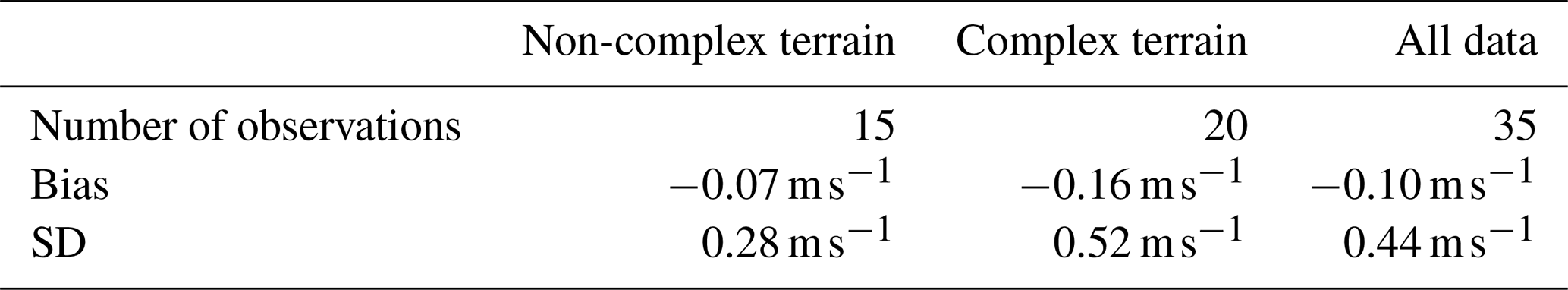
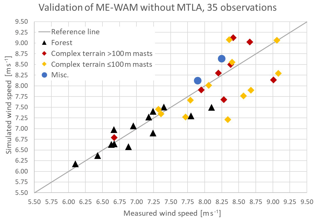
Figure 5Comparison of simulated wind speed (y axis) and measured wind speed at the meteorological mast (x axis) for the 35 data points where MTLA is not applied.
Table 2Validation statistics for the assessment of ME-WAM with MTLA applied for a sample of 45 data points.
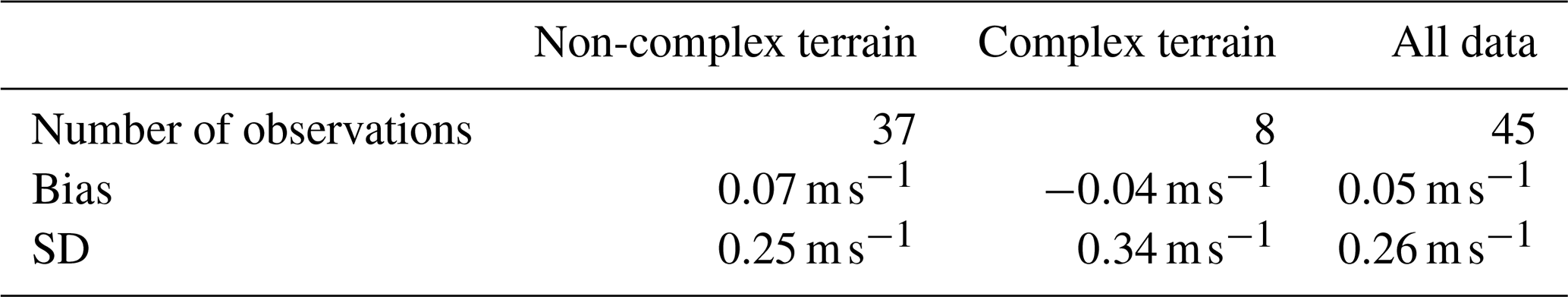
The validation of ME-WAM with the MTLA correction is conducted against a sample of 45 meteorological masts; see Table 2 and Fig. 5. The average wind speed was found to be 0.05 m s−1 higher than the reference sources with a SD of 0.26 m s−1. If the data are binned based on terrain class, we find that the forested and non-complex sites (black and blue markers in Fig. 6) have a bias of +0.07 m s−1 and a SD of 0.25 m s−1 for a sample of 37 data points. The corresponding number for complex terrain is found to be a bias of −0.04 m s−1 and a SD of 0.34 m s−1 for a sample of eight data points.
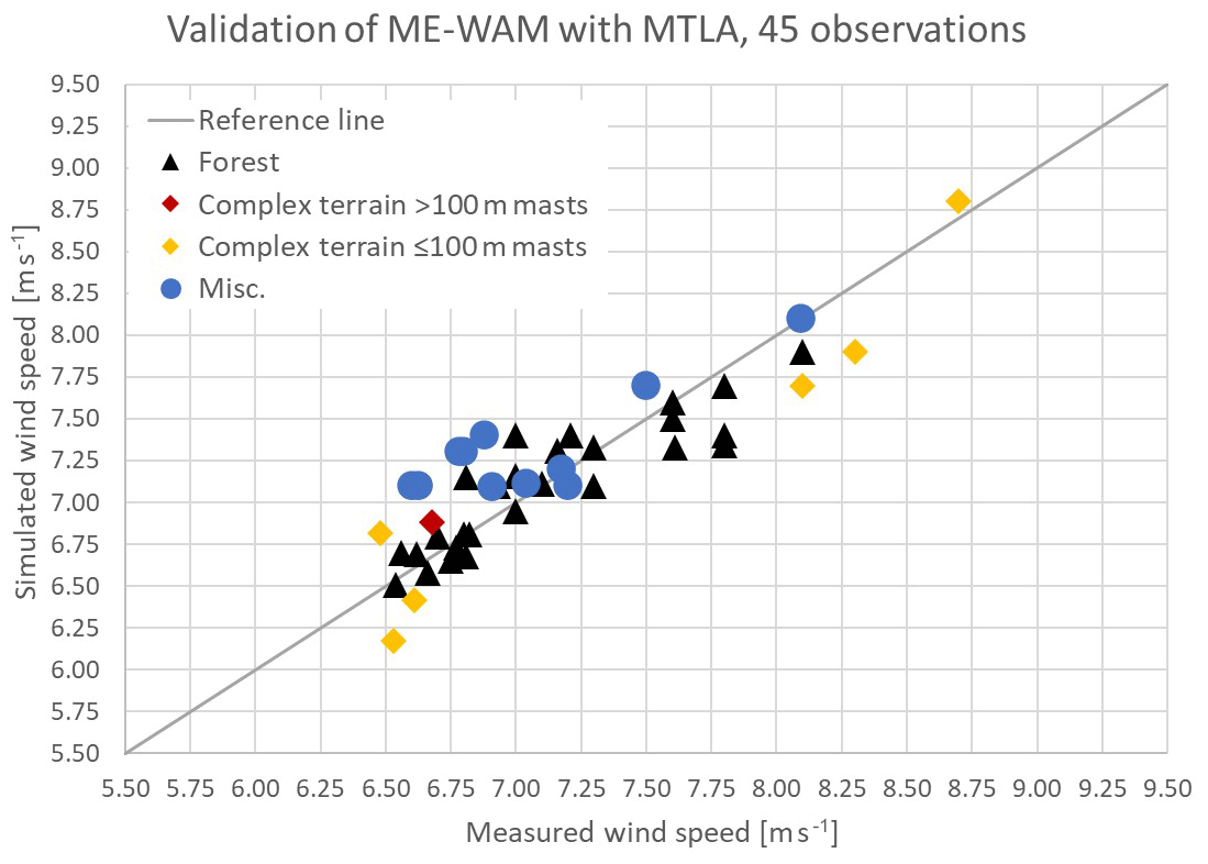
Figure 6Comparison of simulated wind speed (y axis) and measured wind speed at the meteorological mast (x axis) for the 45 data points where MTLA is applied.
Table 3Validation statistics for the assessment of ME-WAM with MTLA applied for a sample of 45 data points.


Figure 7Comparison of simulated wind speed (y axis) and measured wind speed at the meteorological mast (x axis) for 80 data points after MTLA is applied to all data points (note that this includes a reanalysis of the data points in Fig. 5 to include MTLA).
As a final step in the evaluation of the MTLA method, the data from the first ME-WAM validation sample are reanalysed to include MTLA. This evaluation is performed to gain a better significance in the validation, especially for complex terrain where the second dataset contains only eight observations, which makes the conclusions uncertain. Based on 80 data points achieved by combining the two samples, the average wind speed in the ME-WAM analyses is found to be 0.05 m s−1 lower than the reference sources with a SD of 0.28 m s−1; see Table 3. Applying the same binning for terrain class as in the previous analyses, the performance in forested and non-complex sites (black and blue markers in Fig. 7) has a bias of −0.02 m s−1 and a SD of 0.21 m s−1 for a sample of 52 data points. The corresponding number for complex terrain is found to be a bias of −0.12 m s−1 and a SD of 0.35 m s−1 for a sample of 28 data points.
An important metric when using numerical methods for wind resource assessment is the occurrence of large prediction errors. Figure 8 below depicts a box plot of the complete sample of 80 data points using the MTLA method (left) compared to the sample of 35 data points using the ME-WAM model without MTLA (right). It can be seen that utilizing the MTLA method reduces the difference between Q1 and Q3 from 0.53 m s−1 to 0.38 m s−1. The range between P5 and P95 is reduced from 1.30 m s−1 to 0.95 m s−1. This represents a reduction of large prediction errors by 27 %.
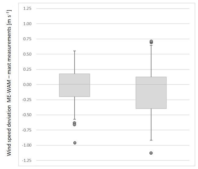
Figure 8Box plot of the derived statistics for ME-WAM with MTLA (left) and without MTLA (right).
The SD of the prediction error for the ME-WAM model compared to field measurements is reduced from 0.44 to 0.26 m s−1 by including the MTLA method based on the blind testing presented above, i.e. a reduction of 40 %. However, as the composition of the validation samples differs, where the validation of the WE-WAM model without MTLA has a higher fraction of complex terrain sites, part of this reduction is likely due to the sample composition. To reduce the effect of the sample composition, the data are binned into classes based on high and low terrain complexity. This results in SDs of 0.28 m s−1 for non-complex sites and 0.52 m s−1 for complex sites when applying ME-WAM without MTLA. With MTLA the numbers are reduced to 0.25 m s−1 for non-complex sites and 0.34 m s−1 for complex sites. The reduction in SD is 11 % for non-complex sites and 35 % for complex sites. This difference is well aligned with expectations as the uncertainty in the data transfer between the WRF and the CFD model is higher in complex terrain. Including multiple transfer locations should therefore have a larger effect in complex terrain.
A re-evaluation of the model results for the 35 data points without MTLA was conducted to gain significance in the predictive ability of the ME-WAM model after the MTLA is implemented. After applying the MTLA to the analyses, the re-evaluated dataset displays similar statistics as the original MTLA test sample with 45 data points. The difference in SD between the two samples is 0.01 m s−1 for non-complex sites and 0.01 m s−1 for complex sites. This adds confidence in the representativeness of the reductions achieved with the MTLA method in the previous test.
Combining the two samples results in a bias of −0.05 m s−1 and SD of 0.28 m s−1 based on 80 data points. The accuracy based on 52 non-complex sites gives a bias of −0.02 m s−1 and a SD of 0.21 m s−1. The corresponding number for complex terrain is found to be a bias of −0.12 m s−1 and a SD of 0.35 m s−1 for a sample of 28 data points.
The variability in the difference between the ME-WAM predictions and the reference data must also be put in relation to the uncertainty of the field data. The uncertainty in the measured long-term-corrected wind speed is estimated to 3 %. The mean wind speed of the sample is 7.5 m s−1, which gives us a SD on the order of 0.23 m s−1. Assuming a Gaussian distribution, this means that theoretically 68 % of the data points should have a measurement error of ± 0.23 m s−1 or less and that 90 % of the data should have a measurement error of ± 0.39 m s−1 or less.
The corresponding numbers for the ME-WAM validation with MTLA show that 68 % of the data points have a difference between ME-WAM prediction and measurement in the range of −0.34 m s−1 to +0.25 m s−1 and that 90 % are within the rage ± 0.48 m s−1. This indicates a distribution that is similar to a Gaussian distribution with a SD of 0.3 m s−1.
As the metric for ME-WAM accuracy inherently includes the variability from the field measurements, and since it is reasonable to assume that the variability of the ME-WAM predictions and that of the measurement are uncorrelated, the variability of the ME-WAM model itself can be derived. Under these assumptions the SD of the ME-WAM model is on the order of 0.2 m s−1. This is an important result as it indicates that the ME-WAM model predictions have a variability and a distribution which are similar to those of a long-term-corrected mast measurement.
This paper describes a method for reducing the uncertainty associated with employing a virtual met-mast approach to couple an NWP model with a CFD model. This is done via a technique where several different locations for performing the data transfer between the NWP and the CFD model are evaluated independently. This enables the analyst to identify and correct for outliers and to obtain multiple realizations of the data transfer step in the modelling chain. The validation shows that this technique results in a reduced variability in the prediction error. The reduction is quantified to 11 % of the SD for non-complex sites and 35 % for complex sites.
The paper also describes a validation of the ME-WAM model with the proposed multiple transfer location (MTLA) method against measurements from 80 meteorological masts. The results show that ME-WAM is able to predict the mean wind speed for the investigated projects with a bias of less than 0.1 m s−1 and a SD of about 0.3 m s−1. The SD is slightly lower in non-complex terrain (0.21 m s−1) and slightly higher in complex terrain (0.35 m s−1). Considering that these numbers include the inherent uncertainty of the reference data, which have an estimated uncertainty of 0.23 m s−1, the ME-WAM model predictions have an accuracy and a variability which are similar to those of a long-term-corrected mast measurement based on this validation.
No public data are available as the validation data are provided anonymously by project developers.
Both authors have been equal parts in developing the ME-WAM methodology and conducting the numerical calculations required for the validation campaign.
The authors declare that they have no conflict of interest.
The authors would like to thank all the wind project development companies that have contributed with measurement data for this validation campaign: Arise, Eolus Vind, Innogy, OX2, Rabbalshede Kraft, Statkraft, Stena Renewable, Vasa Vind, Vattenfall, WPD Scandinavia, and Zephyr.
This paper was edited by Christian Masson and reviewed by Jörn Nathan and one anonymous referee.
Copernicus Climate Change Service (C3S): ERA5: Fifth generation of ECMWF atmospheric reanalyses of the global climate, Copernicus Climate Change Service Climate Data Store (CDS), available at: https://cds.climate.copernicus.eu/cdsapp#!/home (last access: 1 February 2020), 2017.
Draxl, C., Hodge, B. M., Clifton, A., and McCaa, J.: Overview and Meteorological Validation of the Wind Integration National Dataset toolkit, USA, https://doi.org/10.2172/1214985, 2015.
Flores-Maradiaga, A., Benoit, R., and Masson, C.: Enhanced modelling of the stratified atmospheric boundary layer over steep terrain for wind resource assessment, J. Phys. Conf. Ser., 1222, 012005, https://doi.org/10.1088/1742-6596/1222/1/012005, 2019
Giannaros, T. M., Melas, D., and Ziomas, I.: Performance evaluation of the Weather Research and Forecasting (WRF) model for assessing wind resource in Greece, Renew. Energ., 102, 190–198, 2017
Gopalan, H., Gundling, C., Brown, K., Roget, B., Sitaraman, J., Mirocha, J., and Miller, W.: A coupled mesoscale–microscale framework for wind resource estimation and windfarm aerodynamics, J. Wind Eng. Ind. Aerod., 132, 13–26, https://doi.org/10.1016/j.jweia.2014.06.001, 2014.
Hahmann, A. N., Vincent, C. L., Peña, A., Lange, J., and Hasager, C. B.: Wind climate estimation using WRF model output: Method and model sensitivities over the sea, Int. J. Climatol., 35, 3422–3439, https://doi.org/10.1002/joc.4217, 2015.
Haupt, S. E., Kosovic, B., Shaw, W., Berg, L. K., Churchfield, M., Cline, J., Draxl, C., Ennis, B., Koo, E., Kotamarthi, R., Mazzaro, L., Mirocha, J., Moriarty, P., ñoz-Esparza, D. Mu, Quon, E., Rai, R. K., Robinson, M., and Sever, G.: On Bridging A Modeling Scale Gap: Mesoscale to Microscale Coupling for Wind Energy, B. Am. Meteorol. Soc., 100, 2533–2550, https://doi.org/10.1175/BAMS-D-18-0033.1, 2019.
Keck, R. E., Sondell, N., and Håkansson, M.: Verification of a fully numerical approach for early stage wind resource assessment in absence of on-site measurements, Proceedings of Wind Europe conference & exhibition 2–4 April 2019, Bilbao, Spain, PO162, 2019.
Launder, B. E. and Sharma, B. I.: Application of the Energy Dissipation Model of Turbulence to the Calculation of Flow Near a Spinning Disc, Lett. Heat Mass Trans., 1, 131–138, 1974
Mortensen, N. G., Davis, N., Badger, J., and Hahmann, A. N.: Global Wind Atlas – validation and uncertainty, Sound/Visual production (digital), WindEurope Resource Assessment Workshop 2017, 16 March 2017, Edinburgh, UK, 2017.
Mylonas-Dirdiris, M., Barbouchi, S., and Herrmann, H.: Mesoscale modelling methodology based on nudging to reduce the error of wind resource assessment, Conference: European Geo-sciences Union General Assembly, 17–22 April 2016, Vienna, Austria, 2016.
Ohsawa, T., Kato, M., Uede, H., Shimada, S., Takeyama, Y., and Ishihara, T.: Investigation of WRF configuration for offshore wind resource maps in Japan, in: Proceedings of the Wind Europe Summit, Hamburg Messe, 27–29 September 2016, Hamburg, Germany, 26–30, 2016.
Phoenics flow solver: http://www.cham.co.uk/phoenics.php, last access: 30 January 2020.
Prósper, M. A., Otero-Casal, C., Fernández, F. C., and Miguez-Macho, G.: Wind power forecasting for a real onshore wind farm on complex terrain using WRF high resolution simulations, Renew. Energ, 135, 674–686, 2019.
Quon E., Doubrawa P., Annoni J., Hamilton N., and Churchfield M.: Validation of Wind Power Plant Modeling Approaches in Complex Terrain, AIAA Scitech 2019 Forum, 7–11 January 2019, San Diego, USA, https://doi.org/10.2514/6.2019-2085, 2019.
Skamarock, W. C., Klemp, J. B., Dudhia, J., Gill, D. O., Barker, D. M., Duda, M. G., Huang, X.-Y., Wang, W., and Powers, J. G.: A Description of the Advanced Research WRF Version 3, NCAR Tech. Note NCAR/TN-475+STR, 113 pp., https://doi.org/10.5065/D68S4MVH, 2008.
Standen, J., Wilson, C., Vosper, S., and Clark, P.: Prediction of local wind climatology from Met Officemodels: Virtual Met Mast techniques, Wind Energy, 20, 411–430, 2017.
VECTOR AS Windsim: http://windsim.com/ws_docs90/ModuleDescriptions/WindField.html, last access: 31 January 2020.
WAsP: Wind Atlas Analysis and Application Program (WAsP), Risø National Laboratory, available at: http://www.wasp.dk/ (last access: 11 March 2020), 1987.
- Abstract
- Introduction
- Description of the ME-WAM model
- The WRF model
- CFD downscaling with WindSim
- Description of the multiple transfer location analysis (MTLA)
- Description of validation data and method
- Results
- Discussion
- Conclusions
- Data availability
- Author contributions
- Competing interests
- Acknowledgements
- Review statement
- References