Maximal power per device area of a ducted turbine

The aerodynamic design of a ducted wind turbine for maximum total power coefficient was studied numerically using the axisymmetric Reynolds-averaged Navier–Stokes equations and an actuator disc model. The total power coefficient characterizes the rotor power per total device area rather than the rotor area. This is a useful metric to compare the performance of a ducted wind turbine with an open rotor and can be an important design objective in certain applications. The design variables included the duct length, the rotor thrust coefficient, the angle of attack of the duct cross section, the rotor gap, and the axial location of the rotor. The results indicated that there exists an upper limit for the total power coefficient of ducted wind turbines. Using an Eppler E423 airfoil as the duct cross section, an optimal total power coefficient of 0.70 was achieved at a duct length of about 15 % of the rotor diameter. The optimal thrust coefficient was approximately 0.9, independent of the duct length and in agreement with the axial momentum analysis. Similarly independent of duct length, the optimal normal rotor gap was found to be approximately the duct boundary layer thickness at the rotor. The optimal axial position of the rotor was near the rear of the duct but moved upstream with increasing duct length, while the optimal angle of attack of the duct cross section decreased.

1 Introduction

The power output of a wind turbine can be augmented by surrounding it with a duct, typically referred to as a ducted wind turbine (DWT), a diffuser augmented wind turbine, or a shrouded wind turbine. The effect of the duct is to increase the mass flow rate through the rotor. For a given rotor area, significantly more power can be obtained for a DWT compared to an open wind turbine. However, by adding a duct, the total area of the device facing the wind direction is increased. If the power produced per total projected frontal area of the device is calculated for DWTs, often values closer to that of open wind turbines are found (van Bussel, 2007). When nondimensionalized by the kinetic power available in a unit area of freestream, the power per rotor area and power per total area of the DWT are referred to as rotor and total power coefficients and are denoted by C_P and C_P,total respectively. For an open rotor turbine, these two power coefficients are equal. Achieving values of C_P,total greater than the Betz–Joukowsky limit (Okulov and van Kuik, 2012) of 0.593 for a DWT is significant as it means a DWT can capture more power per unit area of the device than an open rotor turbine. Optimization studies of DWTs have shown that DWTs can achieve values of C_P,total beyond the Betz–Joukowsky limit (Aranake and Duraisamy, 2017; Bagheri-Sadeghi et al., 2018). C_P,total not only is a useful metric to compare DWTs with open rotor wind turbines but could be an important design objective in certain problems like fully integrated DWTs for sustainable buildings (Ishugah et al., 2014; Agha and Chaudhry, 2017) or other applications where a designer seeks to maximize the power output from the limited space allocated to a wind turbine.

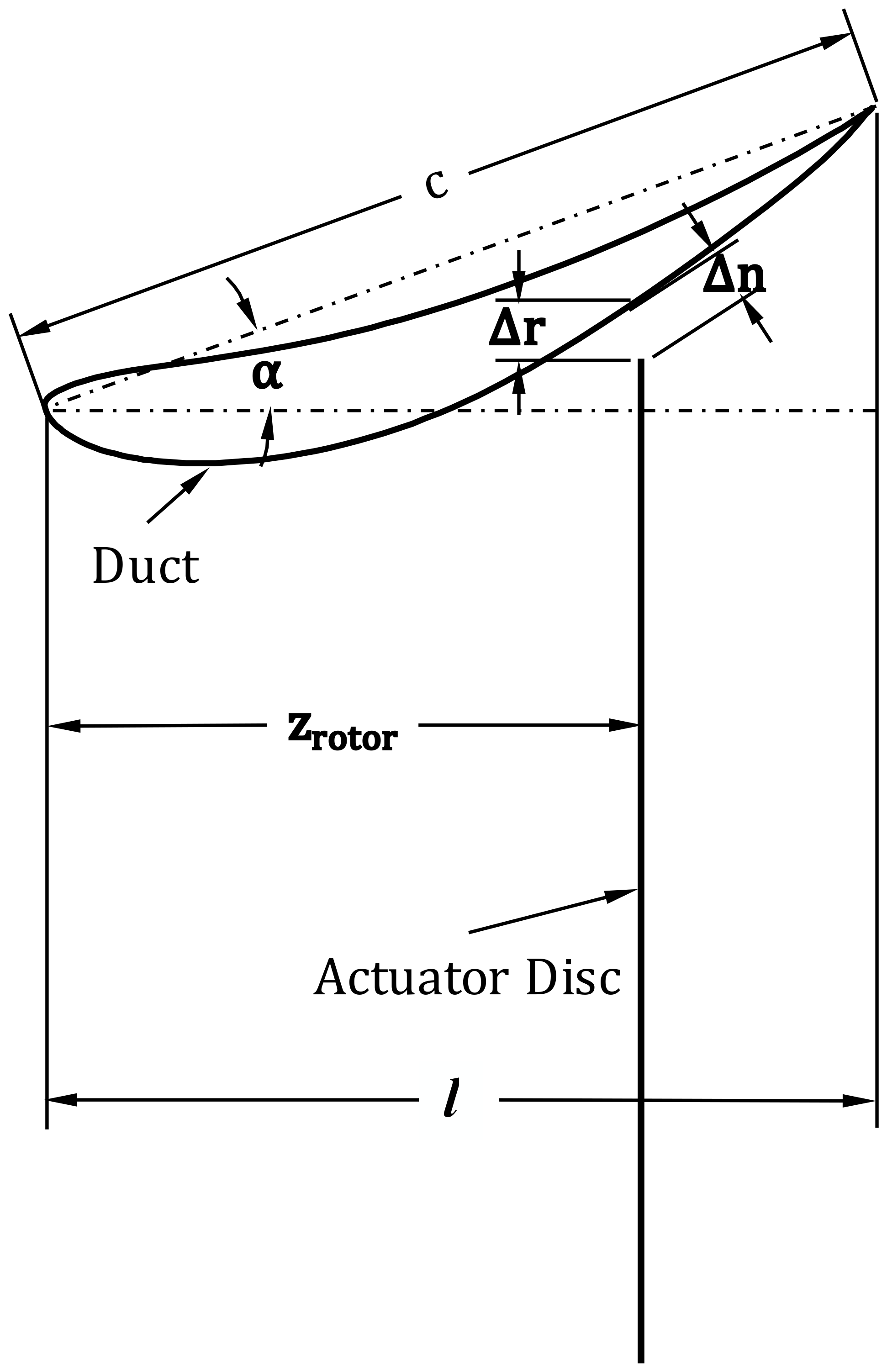
Since the experimental demonstration of the power augmentation provided by shrouding wind turbines (Sanuki, 1950), numerous studies on the design and optimization of the DWTs have been carried out (Lilley and Rainbird, 1956; Igra, 1981; Loeffler, 1981; Gilbert and Foreman, 1983; Georgalas et al., 1991; Politis and Koras, 1995; Hansen et al., 2000; Phillips et al., 2002; Ohya and Karasudani, 2010; Aranake and Duraisamy, 2017; Venters et al., 2018; Bagheri-Sadeghi et al., 2018). Only a few (Aranake and Duraisamy, 2017; Bagheri-Sadeghi et al., 2018; Venters et al., 2018) have used C_P,total as a design metric, while most other studies have focused on maximizing C_P. The design variables of a DWT include the rotor blade design, its axial location (z_rotor), tip clearance or rotor gap (Δn), the angle of attack (α), length (l), and shape of the duct cross section. These design variables can be seen in the schematic shown in Fig. 1 with the rotor replaced by an actuator disc.

Figure 1 The design variables of a ducted wind turbine.

Many of the numerical studies use axisymmetric computational fluid dynamics (CFD) models (Loeffler, 1981; Georgalas et al., 1991; Politis and Koras, 1995; Phillips et al., 2002; Aranake and Duraisamy, 2017; Venters et al., 2018; Bagheri-Sadeghi et al., 2018). If the rotor blades are modeled as an actuator disc, the thrust coefficient can be considered a design variable, and different rotor loadings can be represented by different values of the thrust coefficient (Loeffler, 1981; Hansen et al., 2000; Phillips et al., 2002; Venters et al., 2018; Bagheri-Sadeghi et al., 2018). Similarly, some experimental studies replace turbines with screens of different porosity to study DWTs at various rotor loadings (Igra, 1981; Gilbert and Foreman, 1983). Most simplified theoretical models of DWTs indicate that the optimal power output is achieved at a thrust coefficient of $\mathrm{8}/\mathrm{9}$ similar to open wind turbines (van Bussel, 2007; Jamieson, 2008; Bontempo and Manna, 2020). Bontempo and Manna (2020) reviewed various theoretical models of ducted wind turbines and concluded that they are all equivalent and that their apparent differences are due to different choices of flow parameters used to characterize the effect of the duct (e.g., the exit pressure coefficient, Foreman et al., 1978; or extra back pressure velocity ratio, van Bussel, 2007). They also show that these models are insufficient in predicting the optimal design of ducted turbines as they neglect the dependence of the flow parameters on the thrust coefficient. However, they demonstrated that C_P,total greater than the Betz–Joukowsky limit can be achieved at $C_{\mathrm{T}}=\mathrm{8}/\mathrm{9}$. Bagheri-Sadeghi et al. (2018) reported an optimal value of thrust coefficient close to this value when optimizing for C_P,total using Reynolds-averaged Navier–Stokes (RANS) simulations with an actuator disc model. However, McLaren-Gow (2020) performed axisymmetric inviscid simulations of DWTs with various duct shapes with an actuator disc and concluded that the value of C_T to maximize C_P is lower than $\mathrm{8}/\mathrm{9}$.

As most studies focus on maximizing C_P, with a few exceptions (Georgalas et al., 1991; Politis and Koras, 1995; Venters et al., 2018; Bagheri-Sadeghi et al., 2018), the axial location of the rotor is usually fixed at the smallest cross section of the duct where the maximum velocity is assumed. In our previous paper (Bagheri-Sadeghi et al., 2018), we included the axial position of the rotor as a design variable and compared the optimal designs for maximum C_P and C_P,total. We observed that the optimal axial location of a rotor to maximize C_P or power is close to the duct throat. However, when optimizing for maximum C_P,total, the optimal axial position moves further downstream of the duct throat, which for a given rotor size results in a significantly smaller total area of the device.

The effect of the angle of attack of the duct cross section has been included in most studies (Georgalas et al., 1991; Politis and Koras, 1995; Aranake and Duraisamy, 2017; Venters et al., 2018; Bagheri-Sadeghi et al., 2018). The results of these studies show that power output is considerably sensitive to the angle of attack of the duct cross section and that more power is obtained by increasing the angle of attack of the duct cross section up to the point where the flow separates inside the duct. As noted by Bagheri-Sadeghi et al. (2018), the optimal design of a DWT is on the verge of flow separation, which is often accompanied by a sharp decrease in the power output. Therefore, the accuracy of CFD simulations significantly depends on the accurate prediction of flow separation. The k−ω shear-stress transport (SST) turbulence model (Menter, 1994) is more accurate than the k−ϵ models in prediction of the flow separation for flows with adverse pressure gradients and thus is preferred when RANS simulations are used to study DWTs (Hansen et al., 2000; Bagheri-Sadeghi et al., 2018). This sharp drop in the power, which results in a discontinuity in the objective function, has implications in the choice of optimization method too, as it renders methods assuming a smooth objective function ineffective (Bagheri-Sadeghi et al., 2018).

There are a few studies on the optimization of the shape of the duct cross section for optimal C_P,total such as Aranake and Duraisamy (2017), but the design space is limited by fixing some other design variables. For instance, Aranake and Duraisamy (2017) use a penalty function to avoid large values of the thrust coefficient, and the axial location of the rotor, the chord length of the duct cross section, and the rotor gap were not introduced as design variables. In most studies, a high-lift airfoil with the suction side inside the duct is used as the cross section of the duct (de Vries, 1979). A high-lift airfoil shape creates circulation and thereby increases the mass flow rate through the duct. Further increases in C_P,total could be possible by delaying boundary layer separation, e.g., by using multi-element or slotted ducts (Igra, 1981; Gilbert and Foreman, 1983; Phillips et al., 2002; Hjort and Larsen, 2014), as the optimal design tends to be on the verge of flow separation (Bagheri-Sadeghi et al., 2018). Large flanges are often used at the exit of ducted turbines to further lower the pressure at the exit plane of the duct and increase the swallowing effect. Limacher et al. (2020) showed that large flanges lead to reduced values of C_P,total.

The effect of the rotor gap as a design variable is considered in a few studies (Politis and Koras, 1995; Venters et al., 2018; Bagheri-Sadeghi et al., 2018), and although optimum rotor gaps have been examined (Bagheri-Sadeghi et al., 2018), no conclusions about the optimal rotor gap for optimal C_P,total have been obtained to our knowledge. Lastly, the effect of the duct length for a given rotor diameter on the optimal design of a DWT is only considered in a few works (Georgalas et al., 1991; Politis and Koras, 1995; Ohya and Karasudani, 2010; Venters et al., 2018). Within the range of duct lengths that seem practical (lengths smaller than the rotor diameter), studies suggest that C_P can be increased monotonically by increasing the duct length. However, we are not aware of any studies on the effect of the duct length on the optimal design for C_P,total.

This study investigates the effect of the duct length on the optimal design for maximizing the total power coefficient (C_P,total) of a DWT having the Eppler E423 airfoil as the cross section. This entails identifying whether there is an optimal duct length and how the optimal design variables of a DWT change as the duct length varies. The results show that there is an upper limit to C_P,total for a DWT, which is similar to the Betz–Joukowsky limit for open rotors. The result established here is specific to the Eppler E423 used for the duct cross section, but a similar result should hold for other duct cross sections as well. Additionally, the results indicate that the optimal rotor gap is close to the boundary layer thickness at the rotor independent of the duct length. Furthermore, this paper illustrates how the optimal axial position and the angle of attack of the duct change with increasing duct length.

Figure 2 The computational domain.

The paper is organized as follows: Sect. 2 discusses the CFD model used for RANS simulations including a validation study of the actuator disc model used followed by the details of the DWT design parameterization and the optimization method used. The optimization results and how the optimal design changes with the duct length are discussed in the third section. This section also involves a sensitivity analysis of C_P,total of the optimal design, as well as a comparison of the power per unit device area vs. rotor thrust of the optimal DWT and an open rotor.

2 Methods

Ansys Fluent 17.1 was used to solve the incompressible RANS equations with the k−ω SST turbulence model (Menter, 1994). The computational domain used is shown in Fig. 2, which extends to max(4D,15c) upstream of the rotor and max(8D,25c) downstream of it, where max(x,y) is the greater of x and y, D is the rotor diameter, and c is the chord length of the duct cross section. The flow was considered axisymmetric, and the rotor was modeled as an actuator disc. The pressure drop across each cell of the actuator disc was

$$\begin{array}{}\text{(1)}& \mathrm{\Delta }p={\displaystyle \frac{\mathrm{1}}{\mathrm{2}}}\mathit{\rho }{V}_z^{\mathrm{2}}{C}_{\mathrm{T},\mathrm{rotor}},\end{array}$$

where ρ is the air density and C_T,rotor is the thrust coefficient based on the axial velocity (V_z) at the rotor. The value of C_T,rotor was defined in the fan boundary condition of Ansys Fluent. Using C_T,rotor as a design variable means that the pressure drop across the actuator disc was not constant. However, as it is easier to interpret, all the results are given in terms of the thrust coefficient defined as $C_{\mathrm{T}}=\frac{T}{\frac{\mathrm{1}}{\mathrm{2}}\mathit{\rho }{V}_{\mathrm{\infty }}^{\mathrm{2}}{A}_{\mathrm{rotor}}}$, where T is the thrust force on the rotor, V_∞ is the freestream velocity, and A_rotor is the swept area of the rotor. At the inlet, the freestream values of the turbulence variables were set as ${\mathit{\omega }}_{\mathrm{\infty }}=\frac{\mathrm{5}{V}_{\mathrm{\infty }}}{D}$ and $k_{\mathrm{\infty }}=\mathit{\nu }{\mathit{\omega }}_{\mathrm{\infty }}\times {\mathrm{10}}^{-\mathrm{3}}$, where ν is the kinematic viscosity of air. The flow field of RANS actuator disc simulations are sensitive to freestream values of turbulence variables (Bagheri-Sadeghi et al., 2020), and the values selected correspond to recommended values by Menter (1994). Ansys Fluent uses a cell-centered finite-volume method. The pressure-based solver with the coupled algorithm and Fluent's second-order accurate schemes were used for all flow variables. The values of rotor power output and thrust were monitored to ensure iterative convergence.

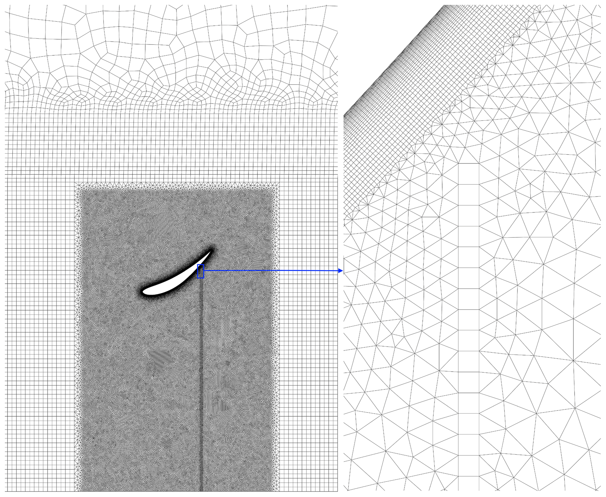
The grid near the duct, which uses both structured and unstructured elements, is depicted in Fig. 3. The average nondimensional wall distance of the first grid point in the boundary layer mesh was $y_{\mathrm{1}}^{+}\approx \mathrm{1}$, and the aspect ratio of the first element on the airfoil was set to about 20. The thickness of the boundary layer mesh was set equal to $\min (\mathit{\delta },\mathrm{0.95}\mathrm{\Delta }n/c)$, where δ is the thickness of the boundary layer over the airfoil estimated from the flat-plate correlation $\mathit{\delta }=\mathrm{1.1}\frac{\mathrm{0.16}c}{R{e}_{\mathrm{c}}^{\mathrm{1}/\mathrm{7}}}$, where the 1.1 factor accounts for the longer curved surface of the airfoil compared to its chord (White, 2006). This prevents the actuator disc from penetrating the boundary layer mesh, which can result in the failure of boundary layer mesh generation. The fan boundary condition in Fluent requires identifying the direction of the positive pressure jump. The use of triangular elements as shown in Fig. 3 between the boundary layer mesh and the outside structured mesh made the grid generation more efficient. However, with the triangular elements used on the fan boundary condition, the specified direction of the fan boundary condition randomly changed from case to case, and sometimes the actuator disc became undesirably distorted. To fix this issue, a thin structured quadrilateral grid was created just downstream of the fan boundary, which is seen in Fig. 3. The width and cell sizing of this thin grid are scaled with $c/D$ to prevent large cells near the boundary layer mesh for smaller ducts.

Figure 3 Grid near the duct and actuator disc.

Two metrics were used to characterize the performance of a DWT: first, the power coefficient based on the swept area of the rotor,

$$\begin{array}{}\text{(2)}& C_{\mathrm{P}}={\displaystyle \frac{P}{\frac{\mathrm{1}}{\mathrm{2}}\mathit{\rho }{V}_{\mathrm{\infty }}^{\mathrm{3}}{A}_{\mathrm{rotor}}}},\end{array}$$

and, second, the power coefficient based on the exit area of the duct,

$$\begin{array}{}\text{(3)}& C_{\mathrm{P},\mathrm{total}}={\displaystyle \frac{P}{\frac{\mathrm{1}}{\mathrm{2}}\mathit{\rho }{V}_{\mathrm{\infty }}^{\mathrm{3}}{A}_{\mathrm{total}}}}.\end{array}$$

C_P,total is a measure of the performance for a given total cross-sectional area of the device, whereas C_P is the performance for a given rotor cross-sectional area.

In order to validate the actuator disc model, the axisymmetric actuator disc without a duct was simulated in the domain shown in Fig. 2. Figure 4 compares the axisymmetric RANS actuator disc simulation results on three different grids with the 1-D actuator disc momentum theory. The coarse, medium, and fine grids had about 1.6×10⁴, 6.5×10⁴, and 2.6×10⁵ cells. The only noticeable difference between the three grids is observed at values of C_T close to 1. At lower values of C_T the RANS actuator disc model and the momentum theory results are visually indistinguishable. For heavily loaded actuator discs with C_T>1, the simple 1-D momentum theory is not valid and empirical correlations are often used (Glauert, 1935; Sørensen et al., 1998).

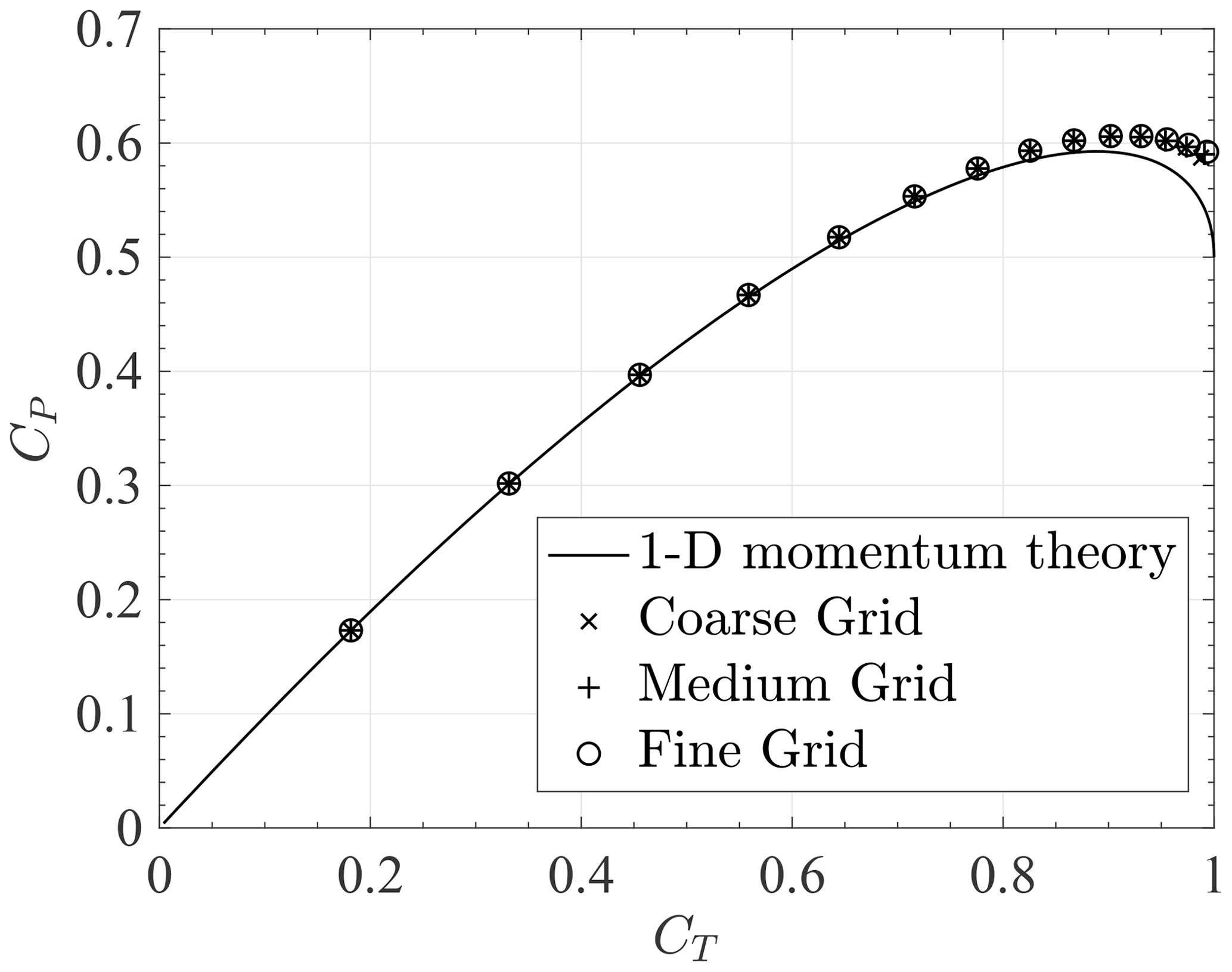
Figure 4 Comparison of axisymmetric RANS actuator disc model with 1-D momentum actuator disc theory.

2.1 Optimization

The performance of the DWT was considered to be a function of a number of design variables, mentioned in the introduction, including the chord length of the duct cross section (c), the thrust coefficient based on the axial velocity at the rotor (C_T,rotor), the angle of attack of the duct cross section (α), the normal rotor gap (Δn), and the axial position of the rotor (z_rotor). These are shown in Fig. 1. The optimization problem was to maximize C_P,total as a function of normalized design variables $\frac{c}{D}$, C_T,rotor, α, $\frac{\mathrm{\Delta }n}{c}$, and $\frac{z_{\mathrm{rotor}}}{l}$, where l is the duct length as shown in Fig. 1. Although the design variable was C_T,rotor, all the results are presented in terms of the easier-to-interpret thrust coefficient based on the freestream velocity $C_{\mathrm{T}}=\frac{T}{\frac{\mathrm{1}}{\mathrm{2}}\mathit{\rho }{V}_{\mathrm{\infty }}^{\mathrm{2}}{A}_{\mathrm{rotor}}}$, where $T=\underset{\mathrm{0}}{\overset{D/\mathrm{2}}{\int }}\mathrm{2}\mathit{\pi }\mathrm{\Delta }pr\mathrm{d}r$. The constraints of the optimization were the positivity of $c/D$, C_T, α, and $\mathrm{\Delta }n/c$ and $\mathrm{0}<z_{\mathrm{rotor}}/l<\mathrm{1}$. The nondimensionalization of the rotor gap by chord length instead of rotor diameter was done to help the optimization process as the optimal normal rotor gap seemed to scale with the chord length of the duct cross section in general. The results given in the next section support this scaling.

When $c/D$ is included as a design variable, one can fix the value of Re_c or Re_D. If Re_D is fixed, the smaller values of $c/D$ result in values of Re_c lower than the operating range of the airfoil for which Reynolds number dependency can be expected. Additionally, the larger values of $c/D$ result in high values of Re_c, which require more computationally expensive boundary layer meshes. For this reason, Re_c was fixed and Re_D was allowed to vary. Re_c was set to a value of 3×10⁵. For the Eppler E423 airfoil used here, the operating range extends to $R{e}_{\mathrm{c}}=\frac{V_{\mathrm{\infty }}c}{\mathit{\nu }}$ as low as 1.4×10⁵. For lower Reynolds numbers, large flow separation is observed before the airfoil can attain its design maximum lift coefficient (Selig et al., 1996; Jones et al., 2008). For the range of chord lengths studied, Re_D varied from 6.0×10⁵ to 6.0×10⁶. The axisymmetric actuator disc model used here is insensitive to the Reynolds number once Re_D is greater than 2000 (Sørensen et al., 1998; Mikkelsen, 2004). Within this range of Re_D, the value of C_P only changed by about 0.07 % when using the fine grid of the actuator disc validation study at $C_{\mathrm{T}}=\mathrm{8}/\mathrm{9}$. Therefore, fixing Re_c should minimize any Reynolds number effects and keep the computational expense of cases with larger $c/D$ manageable. To determine Reynolds number sensitivity, the optimization was repeated at $R{e}_{\mathrm{c}}=\mathrm{1.2}\times {\mathrm{10}}^{\mathrm{6}}$ using the optimal design at $R{e}_{\mathrm{c}}=\mathrm{3}\times {\mathrm{10}}^{\mathrm{5}}$ as the starting point.

The Hooke and Jeeves direct search optimization technique (Hooke and Jeeves, 1961; Kelley, 1999; Kolda et al., 2003) was employed in this study. Our optimization study (Bagheri-Sadeghi et al., 2018) concluded that the flow inside the duct of an optimal design for either C_P or C_P,total as the objective function is on the verge of separation. The flow separation inside the duct can result in a significant drop in power output, and therefore the objective function can be considered almost discontinuous close to such optimal design points. The performance of optimization methods that rely on objective function gradients is affected by the presence of such a discontinuity. The Hooke and Jeeves method, however, is less affected by such discontinuities as it does not assume a smooth objective function and only uses the objective function values to identify if a better design point is found or not.

The optimization technique starts by modifying the initial design, one design variable at a time. These exploratory moves in the design space are called steps in coordinate directions. All the design variables were scaled by their initial values, and the initial step size in each coordinate direction was set to 5 %. Based on the success or failure of these steps in the coordinate directions of the five-dimensional design space, the algorithm creates pattern directions, moves the base point, and increases or decreases the step sizes. The stopping criterion was $\sum _{i=\mathrm{1}}^N\frac{\mathrm{1}}{N}\left|\frac{\mathrm{\Delta }{x}_i}{\mathrm{\Delta }{x}_{i,\mathrm{0}}}\right|<\mathrm{0.1}$, where Δx_i is the step size in each coordinate direction, Δx_i,0 is the initial step size, and N is the number of design variables. This means that the initially small step sizes should on average reduce by an order of magnitude for the optimization to stop. Figure 5 shows the convergence of the optimization technique towards the optimal design. The optimization was repeated with a different initial design, and the optimization approached the same optimal design point.

Figure 5 Convergence of the optimization technique to the optimal design.

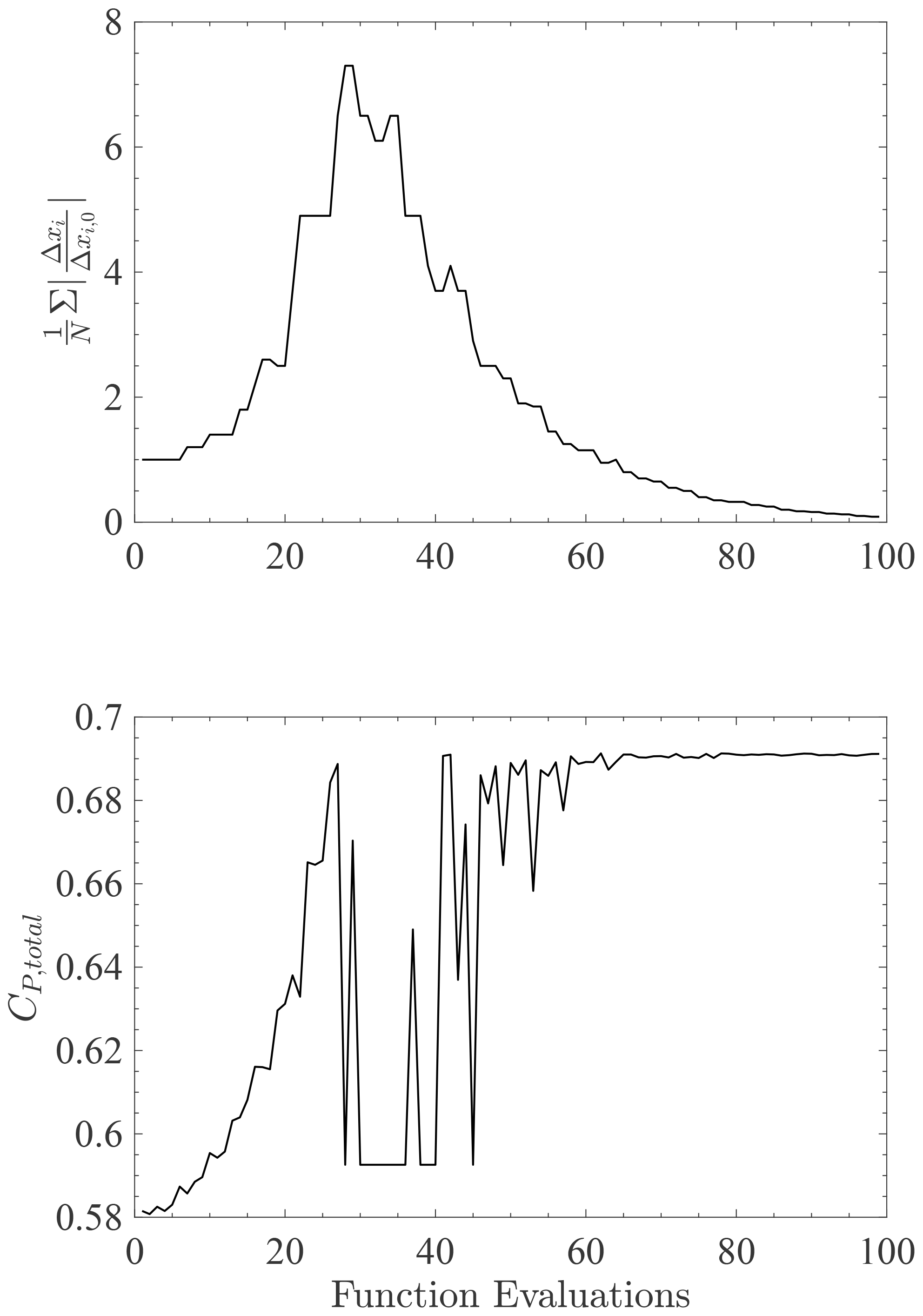
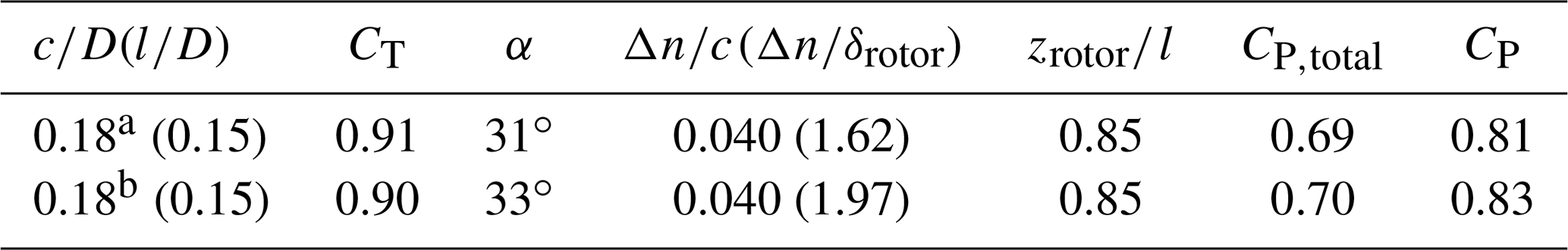
Table 1 The design variables for optimal C_P,total.

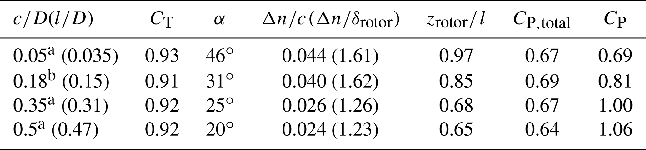
^a The optimization performed at fixed $c/D$ at $R{e}_{\mathrm{c}}=\mathrm{3}\times {\mathrm{10}}^{\mathrm{5}}$.
^b The optimization performed with $c/D$ as a design variable at $R{e}_{\mathrm{c}}=\mathrm{3}\times {\mathrm{10}}^{\mathrm{5}}$.

Figure 6 The power coefficients of designs for optimal C_P,total.

3 Results and discussion

The optimization was performed at a constant $R{e}_{\mathrm{c}}=\mathrm{3}\times {\mathrm{10}}^{\mathrm{5}}$ as described in the Methods section. The optimal design achieved $C_{\mathrm{P},\mathrm{total}}=\mathrm{0.69}$ at $c/D=\mathrm{0.18}$, which corresponds to $l/D=\mathrm{0.15}$. The values of design variables and duct length at this optimal design are given in the second row of Table 1. The optimal design was also simulated on a finer grid with about 1.11×10⁶ cells compared to 2.8×10⁵ cells of the original grid. There was only a 0.03 % difference between C_P,total values. Also, simulating on a larger domain extending 1.4 times further in each direction, the value of C_P,total changed by about −1 %, which was considered sufficiently accurate for the optimization study carried out here.

To verify that there is indeed a maximum in C_P,total with duct length, optimizations were carried out at several other fixed $c/D$ values at $R{e}_{\mathrm{c}}=\mathrm{3}\times {\mathrm{10}}^{\mathrm{5}}$. The optimal designs at these fixed values of $c/D$ are shown in Table 1 as well. Figure 6 shows the power coefficients of the designs for optimal C_P,total. These additional optimization studies confirm that there is an optimal duct length for a DWT that maximizes C_P,total and that this maximum is greater than the Betz–Joukowsky limit. Thus, for applications desiring the greatest power per unit device area, the duct length should be around 15 % of the rotor diameter. As the results here are specific to Eppler E423, further studies are needed to verify this conclusion. The values of power coefficient based on the rotor swept area (C_P) are also shown in Fig. 6 for the designs of Table 1. The values of C_P seem to increase almost linearly with $c/D$. This suggests that significantly larger values of C_P can be obtained by increasing the duct length, but this will result in a lower C_P,total.

Both here and in Bagheri-Sadeghi et al. (2018) the values of optimal C_T were close to 0.9. For all optimal designs of Table 1, the value of the thrust coefficient is close to $C_{\mathrm{T}}=\mathrm{8}/\mathrm{9}$, which is the optimal thrust coefficient of open wind turbines at the Betz–Joukowsky limit. This is in agreement with the momentum analysis and CFD studies of DWTs, which conclude that the optimal C_T values of open and ducted wind turbines are similar (van Bussel, 2007; Jamieson, 2008; Bagheri-Sadeghi et al., 2018).

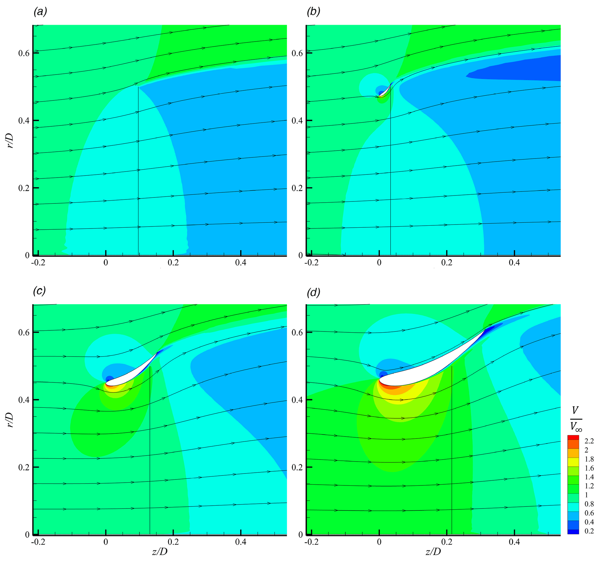
Figure 7 The streamlines and contours of nondimensional velocity magnitude $V/V_{\mathrm{\infty }}$ of (a) the actuator disc, shown by the radial black line, at $C_{\mathrm{T}}=\mathrm{8}/\mathrm{9}$, and the designs for optimal C_P,total at $R{e}_{\mathrm{c}}=\mathrm{3}\times {\mathrm{10}}^{\mathrm{5}}$ at (b) $c/D=\mathrm{0.05}$, (c) $c/D=\mathrm{0.18}$, and (d) $c/D=\mathrm{0.35}$.

The geometry and streamlines of the first three configurations in Table 1 are shown in Fig. 7b–d along with those for an open rotor (in Fig. 7a). The optimal angle of attack of the duct cross section decreased with increasing duct length. For the open rotor, the streamlines close to the tip are at an angle of about 30^∘. Furthermore, at $c/D=\mathrm{0.05}$ almost all of the duct cross section can be considered to be in the vicinity of the strong divergence of streamlines close to the rotor tip. This explains why for the small $c/D=\mathrm{0.05}$ the flow is still attached at α=46^∘. The presence of the small duct with $z_{\mathrm{rotor}}/l=\mathrm{0.98}$ adds extra suction inside the duct without significantly increasing the total area of the device and achieves about 10 % more power per unit device area than an open rotor (i.e., 10 % more than the optimal power output of an actuator disc RANS simulation, which was about 0.6 as shown in Fig. 4). For the optimal design with a variable $c/D$ (i.e., $c/D=\mathrm{0.18}$), the increase in C_P,total is 15 % over an open rotor, and the angle of attack is reduced to 31^∘. Note that the angle of streamlines of the actuator disc with respect to the horizontal decreases further downstream as the rotor wake recovers in Fig. 7. Similarly, further upstream of the rotor for the actuator disc case, the angle of streamlines decreases. At greater duct lengths, the airfoil of the duct cross section becomes less influenced by the presence of the actuator disc and hence the maximum α without a large flow separation decreases. This trend continues for $c/D=\mathrm{0.5}$ (see Table 1).

The optimal normal rotor gap ($\mathrm{\Delta }n/c$) decreased with increasing duct length, but the ratio of the rotor gap to the estimated boundary layer thickness at the rotor ($\mathrm{\Delta }n/{\mathit{\delta }}_{\mathrm{rotor}}$) stayed nearly constant. A smaller rotor gap means a smaller exit area of the duct, and therefore it helps to increase C_P,total. On the other hand, the presence of the rotor gap results in an annular jet of high-velocity air which imparts momentum to the boundary layer and helps the flow stay attached. A Δn that is too small or too large weakens this annular jet. The jet is easier to see in the contour plot of $c/D=\mathrm{0.35}$ in Fig. 7d. For all of the optimal cases shown in Table 1, $\mathrm{\Delta }n/{\mathit{\delta }}_{\mathrm{rotor}}$ was close to 1. When the chord is small relative to D, the dominant length scale is c. This determines the flow scales as well as the boundary layer thickness. Also, note that because Re_c is held constant, the boundary layer thickness at the trailing edge δ scales linearly with c. Therefore, as optimal $\mathrm{\Delta }n/{\mathit{\delta }}_{\mathrm{rotor}}$ is nearly constant, optimal $\mathrm{\Delta }n/c$ only slightly decreases as the optimal rotor position is moved further upstream, resulting in a smaller boundary layer thickness at the rotor (δ_rotor) compared to the trailing edge. This justifies the scaling of Δn by the chord length of the duct.

Similar to Bagheri-Sadeghi et al. (2018), the design for optimal C_P,total resulted in downstream placement of the rotor. The optimal rotor position moved further upstream in the duct as $c/D$ increased. Note that at greater duct lengths the annular jet is stronger as can be seen in Fig. 7. This further upstream placement of the rotor means that the annular jet formed between the rotor tip and duct can exchange momentum with a larger portion of the boundary layer, which may help the DWT attain more power per total unit device area without flow separation.

The sensitivity of the total power coefficient of the optimal design to different design variables x_i is shown in Fig. 8. The greatest sensitivity is to the thrust coefficient of the rotor which matches the results of previous studies (Venters et al., 2018; Bagheri-Sadeghi et al., 2018) and illustrates the importance of rotor design in achieving optimal power output from a DWT (a rotor design approach based on the blade element momentum method using axisymmetric RANS actuator disc simulations as input is discussed by Kanya and Visser, 2018). For α and $z_{\mathrm{rotor}}/l$, an increase in the design variable causes flow separation inside the duct and a significant drop in the power output. This is demonstrated by an increased sensitivity of C_P,total to increase in α and $z_{\mathrm{rotor}}/l$ compared to their reduction. The sensitivity to the reduction in $z_{\mathrm{rotor}}/l$ is mainly driven by changes in the total area of the device rather than changes in the power output. Therefore as concluded in Bagheri-Sadeghi et al. (2018) a smaller DWT with similar power output (i.e., a greater C_P,total) can be designed by placing the rotor further downstream of the duct. The observation that the optimal design is on the verge of flow separation with respect to α agrees with the results of Bagheri-Sadeghi et al. (2018) obtained for the design for optimal C_P. The flow of the design for optimal C_P in Bagheri-Sadeghi et al. (2018) is on the verge of separation with respect to rotor gap and shows little sensitivity to $z_{\mathrm{rotor}}/l$, whereas the optimal design for C_P,total shows the least sensitivity in Fig. 8 to $\mathrm{\Delta }n/c$, and a slight increase in $z_{\mathrm{rotor}}/l$ leads to flow separation.

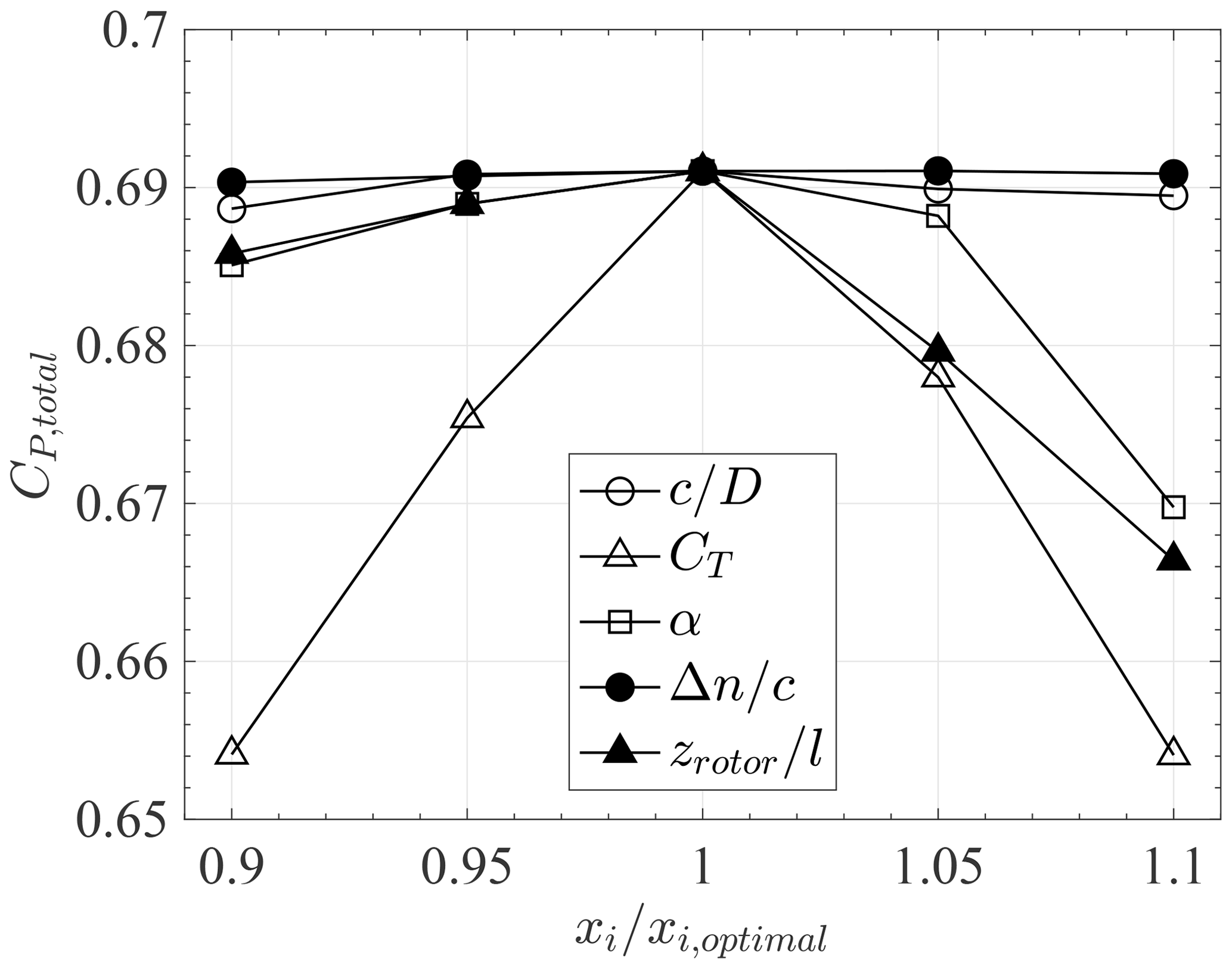
Figure 8 The sensitivity of the total power coefficient of the optimal design to different design variables.

Figure 9 compares the C_P,total vs. C_T curves of the optimal DWT with the RANS actuator disc model. Note that for an open rotor turbine $C_{\mathrm{P},\mathrm{total}}=C_{\mathrm{P}}$. Close to the optimal design, at a given C_T the DWT produces about 15 % more power per unit device area. However, at lower values of C_T, this increase in C_P,total becomes smaller (e.g., at C_T≈0.55 the DWT produces only 6 % more power per total device area). In other words, at lower rotor loadings, the power output of the optimal DWT per total device area approaches that of an open rotor turbine. Generally, when using actuator disc simulations, the increase in velocity of a DWT compared to an open wind turbine should be fixed so the ratio of C_P values (and therefore C_P,total values in Fig. 9 as the A_total is fixed) should be independent of C_T (Hansen et al., 2000). Indeed, if the curves of Fig. 9 were plotted for another DWT design not on the verge of flow separation (e.g., the optimal design but at a reduced α) the ratio of the power coefficients would stay constant. The constant ratio of the power coefficients is not seen here at the optimal design because the optimal design is on the brink of flow separation, and at lower values of C_T the rotor is less effective in keeping the flow attached and the induced velocity decreases. As the thrust coefficient reduces, the high-speed annular jet becomes weaker and therefore cannot keep the flow attached, and gradually the region of flow separation extends further upstream. The flow separation with thrust coefficient reduction is gradual rather than the abrupt separation which can be observed by slightly increasing the angle of attack or $z_{\mathrm{rotor}}/l$ in Fig. 8.

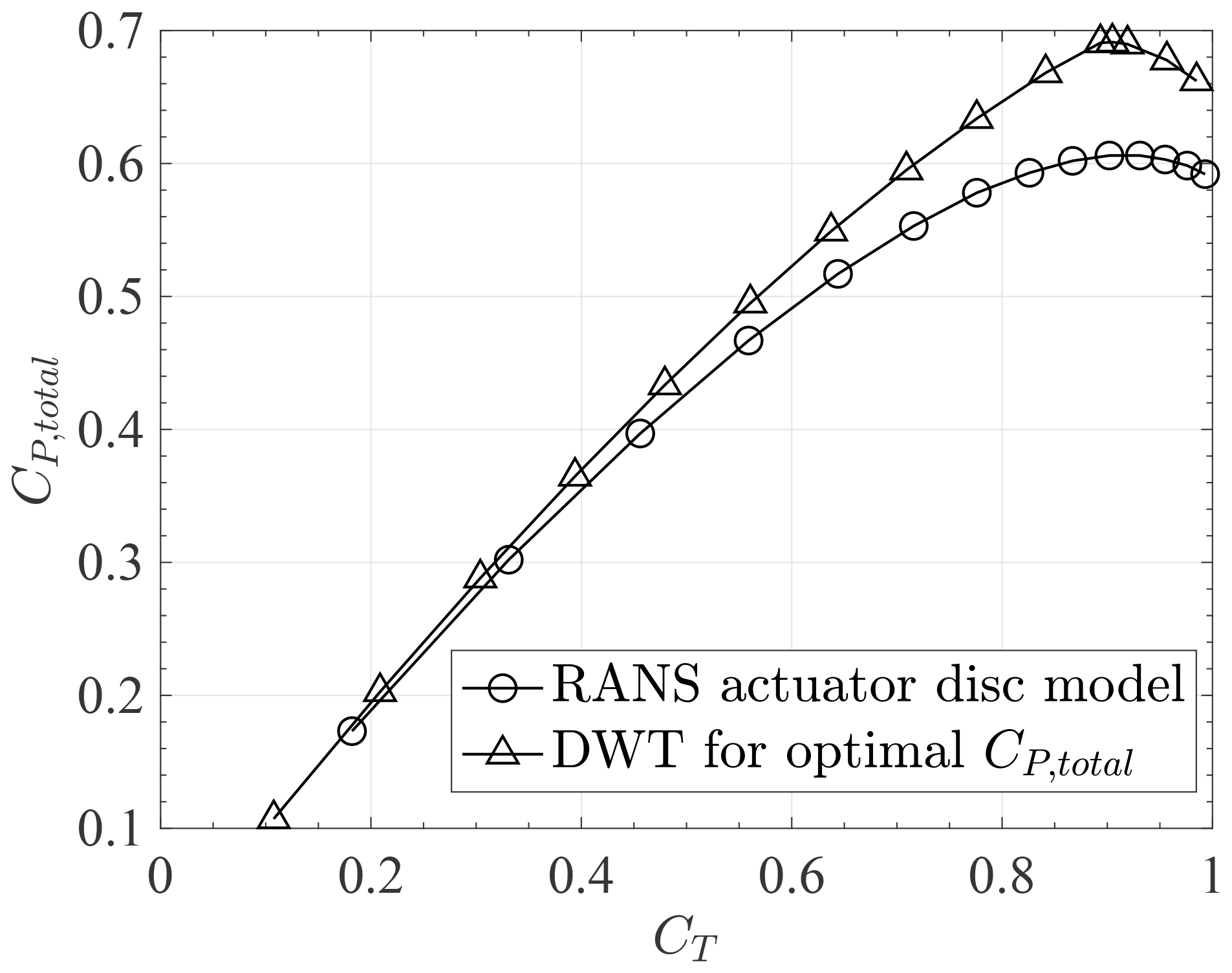
Figure 9 Comparison of C_P,total vs. C_T for RANS actuator disc model and the DWT for optimal C_P,total.

3.1 Reynolds number sensitivity

To examine Reynolds number sensitivity, the simulation of the optimal design was repeated at $R{e}_{\mathrm{c}}=\mathrm{1.2}\times {\mathrm{10}}^{\mathrm{6}}$. The Reynolds numbers used in this study correspond to typical values for DWTs, which typically target residential applications. For example, at a wind speed of V_∞=10 m s⁻¹ at standard sea-level temperature and pressure, the $R{e}_{\mathrm{c}}=\mathrm{3}\times {\mathrm{10}}^{\mathrm{5}}$ design corresponds to c=0.44 m, D=2.4 m, and P=2.3 kW, and $R{e}_{\mathrm{c}}=\mathrm{1.2}\times {\mathrm{10}}^{\mathrm{6}}$ corresponds to c=1.76 m, D=9.8 m, and P=38 kW.

The result of optimization at this higher Reynolds number is shown in the second row of Table 2. The maximum C_P,total slightly increased to 0.70. The optimal value of $c/D$ did not change to the precision of the optimization. The optimal values of $\mathrm{\Delta }n/c$ and $z_{\mathrm{rotor}}/l$ also did not change, and the optimal C_T and α only varied slightly. This confirms that at $R{e}_{\mathrm{c}}=\mathrm{3}\times {\mathrm{10}}^{\mathrm{5}}$ the Reynolds number dependency was small.

Table 2 The Reynolds number sensitivity of optimal design for C_P,total.

^a The optimization performed with $c/D$ as a design variable at $R{e}_{\mathrm{c}}=\mathrm{3}\times {\mathrm{10}}^{\mathrm{5}}$.
^b The optimization performed with $c/D$ as a design variable at $R{e}_{\mathrm{c}}=\mathrm{1.2}\times {\mathrm{10}}^{\mathrm{6}}$.

The contour plot of eddy viscosity ratio $\frac{{\mathit{\mu }}_t}{\mathit{\mu }}$ for the optimal design is shown in Fig. 10a. On the suction side of the duct at $R{e}_{\mathrm{c}}=\mathrm{3}\times {\mathrm{10}}^{\mathrm{5}}$ the turbulence model is activated near the leading edge of the duct. This suggests that the optimal design should be insensitive to Reynolds number. The eddy viscosity ratio at $R{e}_{\mathrm{c}}=\mathrm{1.2}\times {\mathrm{10}}^{\mathrm{6}}$ is shown in Fig. 10b. At this Reynolds number the turbulence model is activated slightly further upstream and the power output increased to C_P=0.82. The small increase can be explained by the reduced flow separation near the trailing edge at this greater Reynolds number, which increased the effective exit area of the duct. Also, note that the turbulence model on the pressure side becomes activated further upstream as well. However, this should not matter in identifying the optimal design as the flow stays attached on the outside of the duct. The k−ω SST turbulence model, with the apparent transition near the leading edge, indicates that the flow is entirely turbulent over the airfoil, and therefore the results should not change significantly even at higher Reynolds numbers.

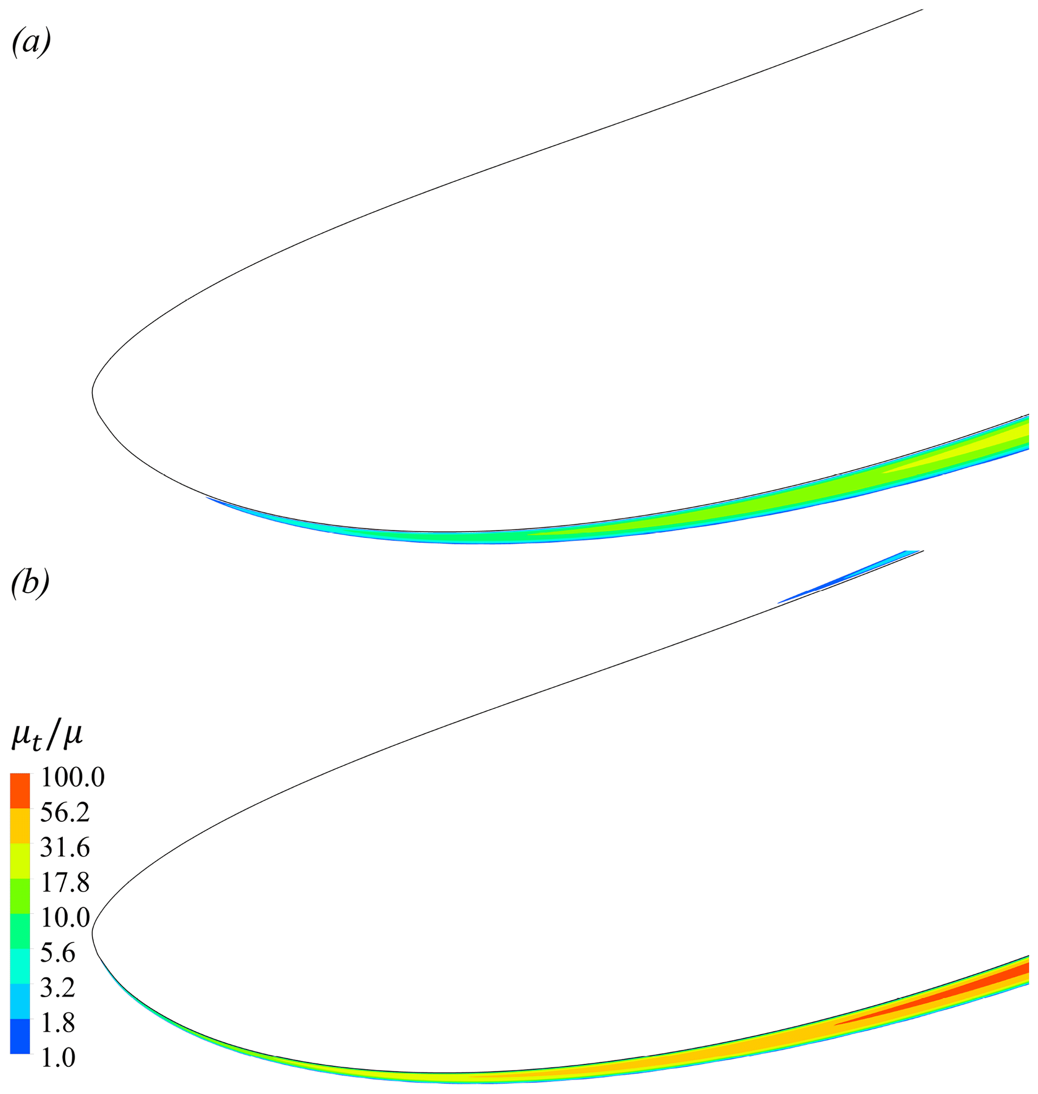
Figure 10 Eddy viscosity ratio contours near the leading edge of the duct for the optimal design ($c/D=\mathrm{0.18}$, C_T=0.91, α=31^∘, $\mathrm{\Delta }n/c=\mathrm{0.040}$, $z_{\mathrm{rotor}}/l=\mathrm{0.85}$) at (a) $R{e}_{\mathrm{c}}=\mathrm{3}\times {\mathrm{10}}^{\mathrm{5}}$ and (b) $R{e}_{\mathrm{c}}=\mathrm{1.2}\times {\mathrm{10}}^{\mathrm{6}}$.

4 Conclusions

The optimal design of a ducted wind turbine with the Eppler E423 airfoil as its cross section was investigated using CFD simulations of axisymmetric RANS equations with the k−ω SST turbulence model and an actuator disc. The total power coefficient characterizing the power output per total area of the device (C_P,total) was used as the design objective. The design variables included the chord length and the angle of attack of the duct cross section, the thrust coefficient, the rotor axial position, and the tip clearance of the rotor.

The results demonstrate the existence of a maximum C_P,total for ducted wind turbines, which sets an upper limit for ducted wind turbines similar to the Betz–Joukowsky limit for open rotors. For the Eppler E423 airfoil, this maximum was obtained for a duct length of about 15 % of the rotor diameter. With this duct length a C_P,total of 0.70 was obtained, which exceeds what can be obtained with an open rotor by 16 %. This is the first time that an optimal duct length has been identified, although the optimization was for C_P,total and not C_P. The value of C_P increased almost linearly with duct length over the range investigated.

Additionally, the results of optimization at fixed $c/D$ suggested that the optimal value of the design variables can significantly change with the duct length. In agreement with previous theoretical and numerical studies, for all duct lengths the optimal thrust coefficient (C_T) was almost 0.9, which is similar to open rotor turbines. The results also showed that the optimal design for C_P,total was most sensitive to the thrust coefficient of the rotor, which indicates the importance of proper rotor design. At lower-than-optimal thrust coefficients, the power per unit device area (C_P,total) of the optimal DWT design gradually approached that of an open wind turbine. This can be explained by considering that the optimal design was on the verge of flow separation and the rotor became less effective in keeping the flow attached as the thrust coefficient decreased.

The optimal angle of attack of the duct cross section decreased significantly with increasing the duct length. Additionally, the optimal design was on the verge of flow separation with respect to the angle of attack of the duct cross section and the axial position of the rotor.

The optimal normal rotor gap was close to the boundary layer thickness at the rotor. Therefore, the optimal normal rotor gap scaled proportional to the chord length of the duct cross section as the turbulent boundary layer thickness almost linearly increases with the chord length of the duct cross section. This gap is needed to create the high-velocity annular jet, which helps keep the boundary layer attached.

The optimal rotor position was at the rear of the duct, but at greater values of duct length it moved further upstream in the duct. This further upstream position was more effective at eliminating flow separation and hence allowed greater values of C_P,total.