the Creative Commons Attribution 4.0 License.
the Creative Commons Attribution 4.0 License.
 | 16 Aug 2021
Vertical-axis wind-turbine computations using a 2D hybrid wake actuator-cylinder model
Edgar Martinez-Ojeda
Francisco Javier Solorio Ordaz
Mihir Sen
The actuator-cylinder model was implemented in OpenFOAM by virtue of source terms in the Navier–Stokes equations. Since the stand-alone actuator cylinder is not able to properly model the wake of a vertical-axis wind turbine, the steady incompressible flow solver simpleFoam provided by OpenFOAM was used to resolve the entire flow and wakes of the turbines. The source terms are only applied inside a certain region of the computational domain, namely a finite-thickness cylinder which represents the flight path of the blades. One of the major advantages of this approach is its implicitness – that is, the velocities inside the hollow cylinder region feed the stand-alone actuator-cylinder model (AC); this in turn computes the volumetric forces and passes them to the OpenFOAM solver in order to be applied inside the hollow cylinder region. The process is repeated in each iteration of the solver until convergence is achieved. The model was compared against experimental works; wake deficits and power coefficients are used in order to assess the validity of the model. Overall, there is a good agreement of the pattern of the power coefficients according to the positions of the turbines in the array. The actual accuracy of the power coefficient depends strongly on the solidity of the turbine (actuator cylinder related) and both the inlet boundary turbulence intensity and turbulence length scale (RANS simulation related).
- Article
(5261 KB) - Full-text XML
-
Supplement
(2626 KB) - BibTeX
- EndNote


The modeling of vertical-axis wind-turbine (VAWT) farms has lacked researched in the last years compared to horizontal-axis wind turbines (HAWTs). The complexity of the models ranges from simple momentum models to full-rotor RANS (Reynolds-averaged Navier–Stokes equations) or LES (large-eddy simulations) simulations. While simple models are computationally inexpensive, they lack accuracy and rely on various semi-empirical corrections which may not be valid for all cases; high-fidelity simulations are simply out of the scope of many researchers and scientists due to the tremendous computational requirements.
This work proposes an actuator model integrated within an OpenFOAM solver that relies on replacing the turbine by volumetric forces exerted on the fluid; this approach eliminates the need of highly resolved meshes around the blades, thereby reducing the mesh size considerably. The forces are modeled using the steady-state actuator-cylinder model (Madsen, 1982), although any other model can be employed. This approach is two-dimensional and the computational time needed for simulating a wind farm ranges from minutes to hours; moreover, the fidelity is superior to that of simple momentum models since the viscous wake is resolved by the RANS simulation. This proposed model provides the capability of serving as an optimization tool for vertical-axis wind-turbine farms. The models that have been used for wind farm modeling will be listed according to complexity; their benefits and caveats will be listed.
The first category belongs to models using the momentum theory or potential flow theory. One of the simplest wake model is the Jensen model (Jensen, 1983), which is able to describe the wake shape provided the thrust coefficient and induction factors are given. The rate of growth of the wake depends on empirical constants. The model can be extended to multiple turbines using a superposition technique. Although it was originally developed for HAWTs, some researchers have developed similar models for VAWTs (Abkar, 2019), achieving good results for the wake shape. Potential flow models try to emulate the wake of a turbine by superposing many different potential flows such as a uniform stream, a dipole and a vortex (Whittlesey et al., 2010). The wake deficit can be modeled as a probabilistic density function, and it is simply subtracted from the flow field. This model has also been extended to multiple-turbine environments (Araya et al., 2014), but it is still very problem-dependent and needs much more calibration since it is unable to model viscous effects.
The next category belongs to actuator models. As it was said before, these models rely on replacing the turbine by volumetric forces. Svenning (2010) has successfully implemented a RANS actuator disc model for a HAWT in OpenFOAM. The model is explicit, and it requires the values of thrust and torque; although it can be extended to multiple turbines, it relies on the assumption of all turbines having the same thrust and torque, which may not be entirely true for turbines in the back rows. Bachant et al. (2018) have also developed actuator line models for both HAWTs and VAWTs with the option of using either RANS or LES. Shamsoddin and Porté-Agel (2016), Abkar (2018) and Mendoza and Goude (2017) have also performed LES simulations of actuator line models on a single VAWT. An interesting multi-turbine simulation using an actuator line model was done by Hezaveh et al. (2018); the study works on the effect of clustering the turbines in order to increase the power density.
The last category of models employs full-rotor RANS simulations. Works on multiple VAWTs can be found in Zanforlin and Nishino (2016), Bremseth and Duraisamy (2016) and Giorgetti et al. (2015). Recently, a very interesting study by Hansen et al. (2021) was done on pairs and triplets of VAWTs; the study claims that a 15 % increase in power can be achieved if turbines are placed closer. Although these claims are done on the basis of 2D simulations, it is not certain whether this effect may scale to a wind farm.
The current RANS-AC has the potential of modeling entire wind farms without relying on empirical corrections for the wake or without the need of HPC (high-performance computing). Moreover, only simple input data must be entered, namely the geometrical and operational parameters and inlet boundary conditions for the simulation.
This section first presents the theory behind the AC model, then the justification of the linear solution is described in detail and a validation for the stand-alone AC is included. The last part deals with the details of the RANS-AC implementation in OpenFOAM.
2.1 Stand-alone actuator-cylinder model
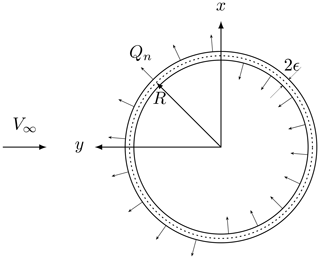
The VAWT can be modeled as a hollow cylinder upon which radial volume forces fn(θ) act. This will create a pressure jump across the entire surface (notice that the cylinder is merely an abstraction; it does not exist materially). The turbine's blades are responsible for these radial forces. Figure 1 shows a cross section of an infinite long cylinder (in the z direction), the incoming wind velocity is V∞, 2ϵ is the cylinder's thickness and R is the radius. Madsen (1982) showed that
where Qn is the normal load per unit length exerted on the fluid at angular position θ averaged over one revolution 2πR. The AC coordinate system is x and y. The governing equations are those of continuity and the steady-state Euler equations. Velocities in the x and y directions are non-dimensionalized by the incoming wind velocity V∞; lengths are non-dimensionalized by the wind-turbine radius R, and pressure is non-dimensionalized by .
The Euler equations are applied to the entire field, and the volume forces are represented by the forces exerted by the blades. The final form of the solution is shown in Eqs. (2a) and (2b), which allow calculation of the perturbation velocities wx and wy; N is the number of evaluation points, θ is the angle of the current evaluation point and ϕ is a dummy angle used for integration purposes. The turbine rotates counterclockwise. This form only includes the linear part, although a correction is made to make up for the non-linear terms. When the evaluation takes place inside the hollow cylinder, term I must be included; on the other hand, if the evaluation point is located in the wake (the leeward part of the cylinder), both I and II must be included in the equation. Li (2017) provides a useful discretization scheme assuming the forces are piecewise constant.
These equations can be put in matrix form using influence coefficients that depend on geometrical variables that have to be computed only once and a column vector Qn. Equation (2a) and (2b) can predict the perturbation velocities along the hollow cylinder provided the forces are known, for which the blade element theory is needed. The free stream velocity V∞ is broken down into its x and y Cartesian components so that they can be projected along the cylinder tangential and normal directions. Note that α is the angle of attack with respect to the chord of the blade, ωR is the tangential velocity of the blade due to rotation, Vt and Vn are the airflow tangential and normal velocities, and Vrel is the relative velocity. Sometimes the chord is pitched slightly by an angle δ.
The normalization of the loads can be found in Li (2017), and it will be outlined briefly here for the case of a counterclockwise-rotating turbine. From now on, all variables will be non-dimensional (written in lowercase). The local x and y velocities can be decomposed into the normal and tangential velocities.
The rotational speed of the rotor normalized by V∞ is , which is a common characteristic parameter of wind turbines called the tip-speed ratio denoted by λ. The normalization of the relative speed and α are
The aerodynamic forces are
The lift and drag coefficients can be obtained from a lookup table as a function of α and Reynolds number. Some common NACA profiles have plenty of experimental data and can be found in Sheldahl and Klimas (1981) at high Reynolds numbers and for an ample range of α. Finally the normal and tangential forces exerted on the cylinder become
The turbine σ is given by , which can be interpreted as the blades' area per unit length divided by the turbine swept area per unit length. It is important to keep σ low; otherwise the basic assumptions about the model break down since effects such as flow curvature and flow distortion are not taken into account. The model does not guarantee any results whatsoever if high-solidity rotors are used. Cheng (2016, p. 40) uses the AC model in his PhD thesis, and the solidity values encountered there are fairly low – around 0.12 for a large two-bladed VAWT; Paraschivoiu (2002, p. 169) also employs low-solidity turbines in the development of his double-multiple stream-tube model, and the values of σ do not go beyond 0.22. The problem of solidity becomes important in small turbines as they have a large ratio. According to Migliore et al. (1980), these blades are subjected to a curvilinear flow which alters the boundary layer of the airfoil. Kinematic analysis from Migliore et al. (1980) also shows that the angle of attack and the relative wind velocity are dependent on the azimuthal angle, the tip-speed ratio and the chord-to-radius ratio; therefore α and vrel can vary significantly chordwise since any point on the blade has a unique radial distance. By employing conformal mapping techniques, it is possible to transform the airfoil in the curvilinear flow to a virtual airfoil in a rectilinear flow. The transformation introduces a camber and an additional angle of incidence – namely virtual camber and virtual incidence – which are also dependent on the azimuthal angle, although they can be averaged by the mean value of one revolution. Thus it is shown in Migliore et al. (1980) that these virtual airfoils have lift at α=0; therefore the CL vs. α curve is shifted upwards depending on the value of . Not only the lift coefficient is affected but also the stall angle, which occurs much earlier as in the original airfoil without a camber; this premature stall deteriorates the efficiency of the wind turbine. Results from wind turbines with values of and each in Migliore et al. (1980) show that the power coefficient is strongly dwindled as increases. In summary, results from the AC model using relatively-high-solidity wind turbines will certainly miscalculate the angle of attack to a certain degree, thus overestimating the power coefficient of the turbine.
The perturbation velocities can be determined if the forces are known, while the forces also depend on the perturbation velocities. The solution is iterative: first, the perturbation velocities are set to zero, then the aerodynamic coefficients are computed as well as Qn and Qt. Equations (2a) and (2b) are used to find the perturbation velocities, and the process is repeated until convergence.
2.2 The linear correction
The aforementioned equations are only valid for low-loaded rotors (thrust coefficient), with the model including only the linear part stops being accurate at high loads; however, a relation between the induction factor a and the thrust coefficient CT was found for the linear solution. Equating this thrust coefficient to an empirical thrust coefficient from the momentum theory yields a correction factor for the induction factor at high loads. The perturbation velocities are all multiplied by the correction factor ka. The procedure is straightforward and can be found in Li (2017), Madsen et al. (2013), Ning (2016), Cheng et al. (2016) and Cheng (2016). There are, however, many empirical corrections. Madsen et al. (2013) provide the following equations for ka.
where k3=0.0892, k2=0.0544, k1=0.251 and k0=−0.0017. Ning (2016) cites the following equations.
The thrust coefficient can be obtained using the following equation, which can be found in Li (2017). This equation is valid for counterclockwise and clockwise rotation.
2.3 Validation against a 1.2 kW Windspire turbine
The Windspire was chosen for validation because it will be used throughout this work; therefore the results of the AC model will be compared against experimental data. Ideally, it would be better to validate against a low-solidity turbine since it meets the requirements of the AC model; nevertheless, the Windspire turbine will be used despite it having a solidity of σ=0.32. According to Zanforlin and Nishino (2016), the turbine is kept at an optimal tip-speed ratio λ=2.3 up until 10.6 m s−1; after this point the rotational speed is kept constant and λ begins to decrease. The turbine's radius is R=0.6 m, the height is H=6.1 m, the number of blades is N=3, the chord is c=0.128 m and the airfoil is a DU06W200 section derived from a NACA0018 section, except the maximum thickness is 20 % and little camber is added.
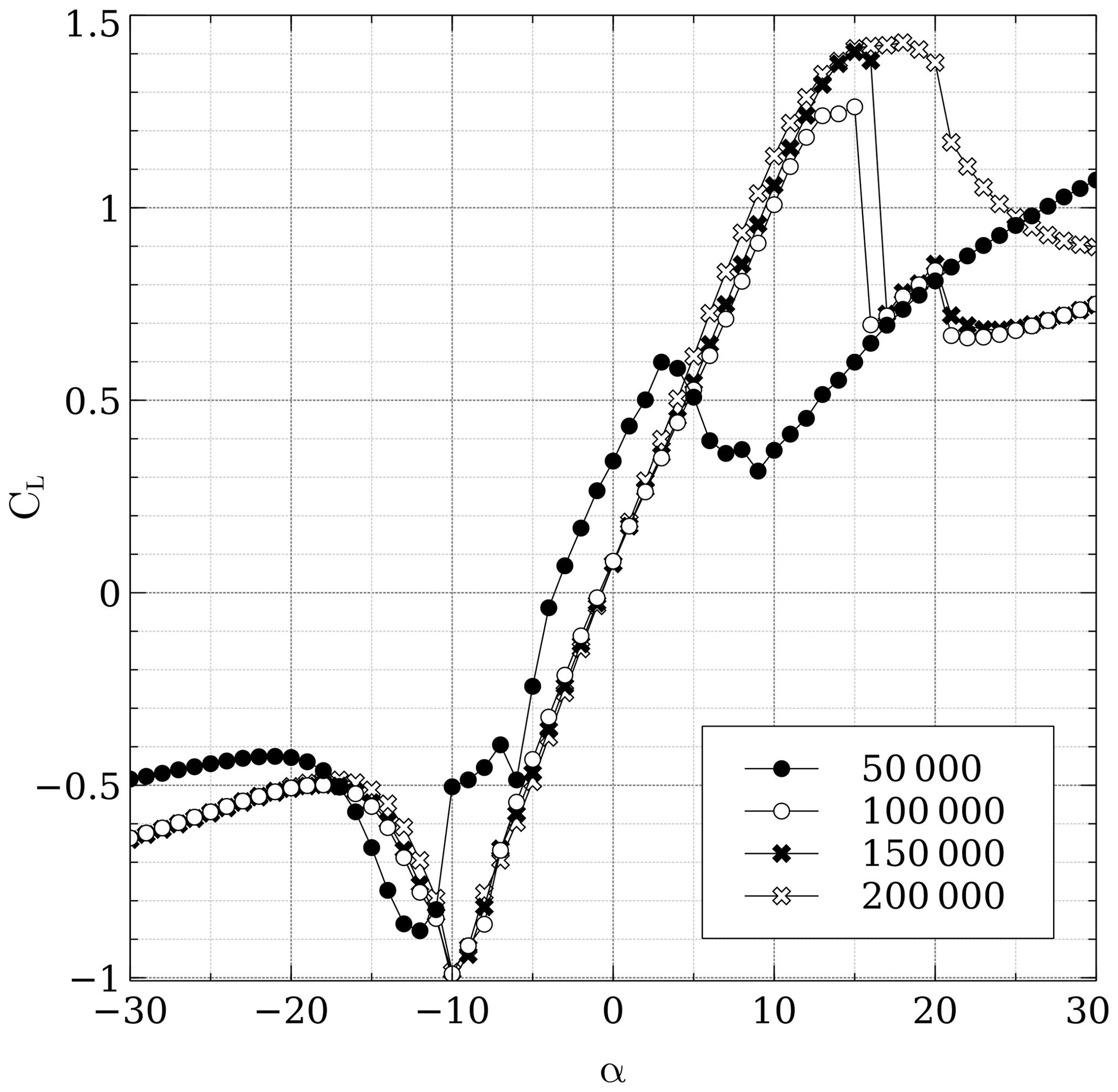
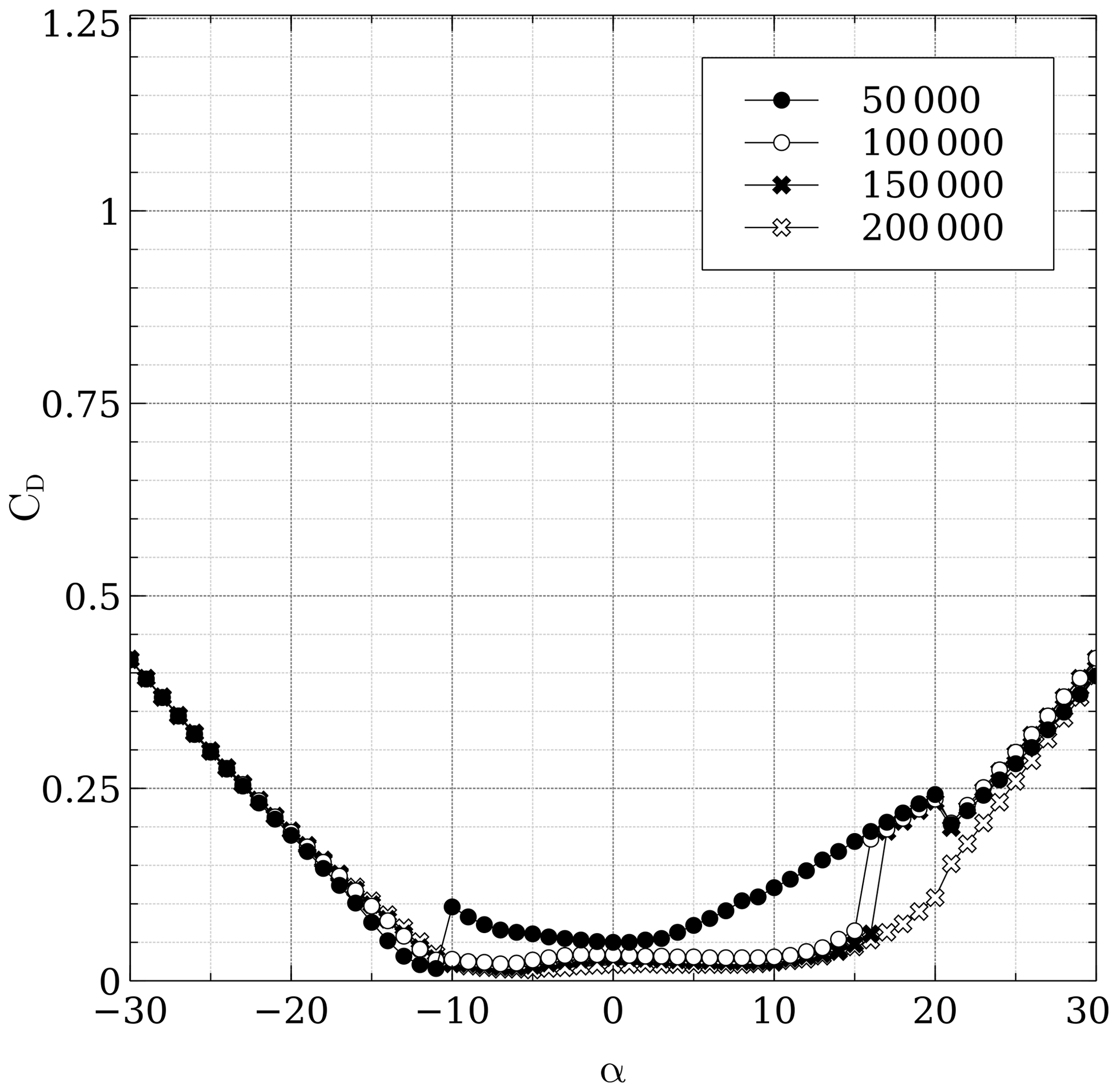
A particular challenge was to find polars for the DU06W200. Claessens (2006) provides both theoretical and experimental data for Reynolds numbers of 300 000 and 500 000 but does not give information whatsoever for a Reynolds number below 300 000; the turbine's global Reynolds number at 8 m s−1 is , with ω being the rotational speed. It was then decided to use polars from the software QBlade (Marten et al., 2013), which is based on a vortex panel code derived from the MIT code Xfoil (Drela, 1989). QBlade is able to predict both drag and lift coefficients at angles of attack below stall; for ranges above stall, an extrapolation can be done based on the Montgomerie extrapolation method, which is more accurate (at least in this case) than the Viterna model. It was observed that the Montgomerie model predicted better the shear drop in lift after stall has occurred. Figures 2 and 3 show the polar for both the lift and drag coefficient at the typical Reynolds numbers encountered by this turbine; QBlade seems to have trouble at low Reynolds numbers, and instabilities are manifested in the zone just before stall plus the fact that the slope before stall is not always linear and presents jagged segments; despite the shortcomings, polars at Re=50 000 Re=100 000, Re=150 000 and Re=200 000 were included. At higher Re it was found that QBlade overestimated lift and could not predict well the shear drop of lift after stall according to wind tunnel data from Claessens (2006).
No attempt was made to introduce dynamic stall or flow curvature effects. Dynamic stall models can conflict with the AC model according to Li (2017). As for flow curvature due to the turbine's – which is above 0.075 and 0.11 in Paraschivoiu (2002, p. 169) and Cheng (2016, p. 40), respectively – it was decided not to employ any model due to the increase in computational cost. Li (2017) uses Migliore's model, which computes the shape of a virtual airfoil with an added camber (the original airfoil in a curved flow is mapped to a cambered airfoil in a straight flow); consequently, the lift and drag coefficients have to be recomputed according to the shape of the virtual airfoil – this needs models such as the vortex panel model, which can be expensive considering that the panel model has to be called for every azimuthal position times the number of iterations.
The results from the AC model were compared against data from AC model results provided by Ning (2016); experimental data are also available. Equations (15) and (16) were used for the linear correction. Figure 4 shows how both AC models overpredict the CP. This overestimation must be in part because both AC models employ limited polars – e.g., Ning (2016) using wind tunnel data at Re=300 000 and this work using data ranging from Re=50 000 to Re=200 000, thereby neglecting the fact that at lower wind speeds Re is much lower. The other reason must be because of the fact that the model is only two-dimensional, and no effects from struts, tower, tip losses, and flow curvature and dynamic stall are included. There is an overall good tendency; the results from the current work and the experimental data both peak at 10 m s−1. Without accurate polars from wind tunnel measurements, it is hard to get accurate results; the CP is therefore very sensitive to the polars, and care must be taken when interpreting the lift and drag coefficients.
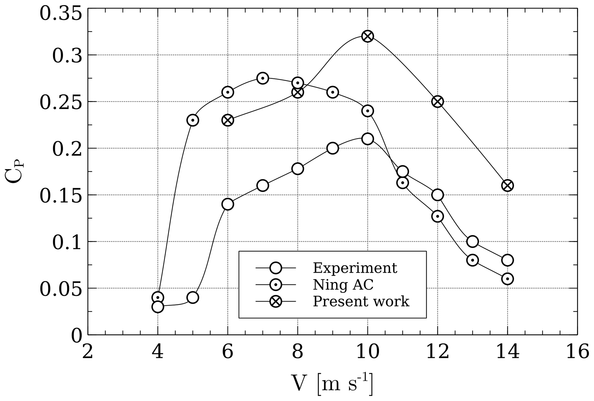
Figure 41.2 kW Windspire turbine validation and comparison. λ is kept at 2.3 up until 10 m s−1.
2.4 RANS-AC implementation
The AC model can be incorporated into one of the OpenFOAM solvers by taking advantage of the source terms in the Reynolds-averaged Navier–Stokes equations. The solver used is called simpleFoam (Moukalled et al., 2016), which solves the steady-state incompressible Navier–Stokes equations for turbulent flows. A new solver called actuatorCylinderSimpleFoam was made using the simpleFoam solver as a template. Whereas the solver needs minimal modification, the AC routines took most of the work. These routines are placed in separate files. The k–ϵ turbulence model is preferred since it has proven to yield relatively good results in environmental flows such as wakes (Bardina et al., 1997; Wilcox, 1998). Algorithm 1 shows the process followed by the new solver.
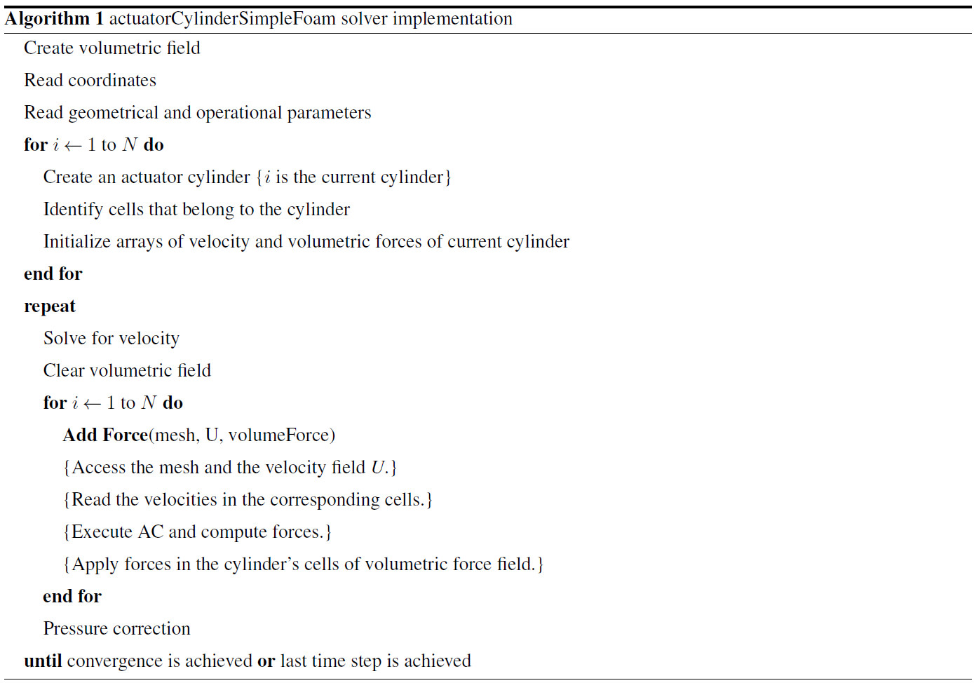
Notice that N is the number of cylinders (turbines); each cylinder has a set of corresponding cells where the velocity is read and then passed to the AC routine, which computes the volumetric forces and passes them back to OpenFOAM using the function Add Force. The thickness of the cylinder is subjective, and it will be explained in the next sections. The way the volumetric forces are calculated by the RANS-AC is by assuming that they do not vary significantly across the thickness of the cylinder; therefore Eq. (1) becomes Eq. (18), where Δr is the thickness of the cylinder, and fn(θ) are the volumetric forces normal to the cylinder as a function of the azimuthal angle. These normal forces have to be projected in the x and y direction of the volumetric field of the simulation.
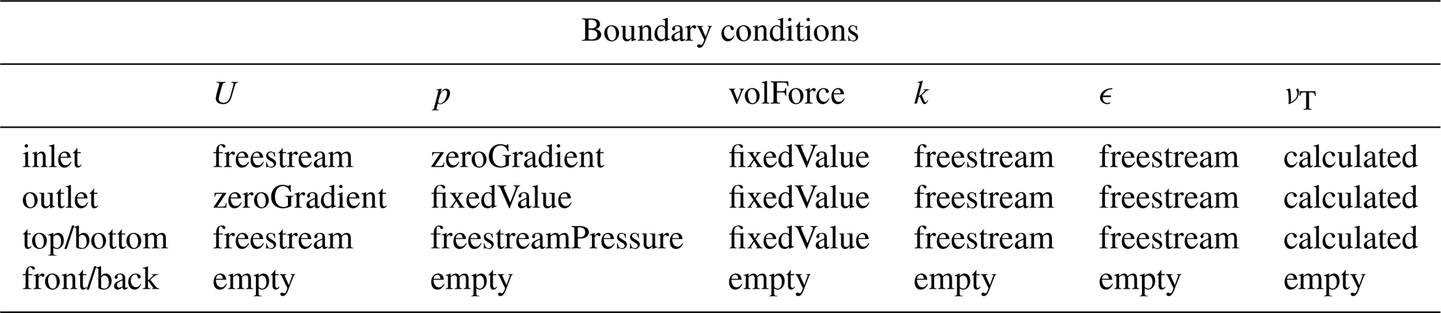
Table 1Boundary conditions at time 0 for the computational domain.
2.5 RANS-AC verification against AC model
In order to prove that the RANS-AC has been implemented correctly, the power coefficient of the RANS-AC will be compared against that of the stand-alone AC model. A sensitivity analysis concerning the thickness of the cylinder and the turbulence intensity I at the inlet of the domain will be discussed. A uniform mesh was chosen for simplicity. Although OpenFOAM is provided with mesh refinement utilities, the refined mesh is inevitably three-dimensional due to the meshing algorithm, which is even more computational expensive; therefore the refined mesh was discarded. The boundary conditions are inlet, outlet, top and bottom, and back and front. Table 1 shows the boundary conditions for every variable OpenFOAM has to compute.
It must be clear that the simpleFoam solver interprets p as since the RANS equations are divided by ρ due to the flow being incompressible. Free stream conditions act like a zero-gradient condition when the flow comes out of the domain and act like a fixed value when it is not; it is a kind of inlet–outlet condition in case of having flow reversal. The freestreamPressure is an outlet–inlet condition that uses the velocity orientation to act either as a zero-gradient condition or a fixed-value condition. The empty boundary condition means that nothing is calculated at those faces; this is only valid for two-dimensional cases with one cell in the third direction.
Table 2RANS-AC results from two different meshes verified against the stand-alone AC.

In summary, all variables have to be initialized at time 0 in the domain. In order to initialize the values of all variables, a set of equations is needed. Equations (19)–(22) are the turbulence length scale, the turbulent kinetic energy, the turbulent kinetic energy dissipation rate and the turbulent viscosity, respectively. The least intuitive is l; this value is taken from Versteeg and Malalasekera (1995, p. 66) based on the case of a wake flow, where L is the wake width which will be taken as the diameter of the cylinder. Cm is just a constant set to 0.09 by default.
The RANS-AC was verified against the Windspire turbine using a fine mesh and a coarse mesh. The mesh size was based on enclosing the cylinder in a n×n cell square; the rest of the domain was meshed accordingly. Distances from the inlet to the turbine could range from 3 to 5 D (diameters) as well as distances from the turbine to the sides. Distances from the turbine to the outlet could be shorter than 10 D. No impact was observed in the CP. Table 2 shows the comparison of the power coefficients as well as the mesh parameters. No significant difference was observed between both meshes, although both meshes underpredicted CP at 14 m s−1. The number of time steps is dependent of the inlet velocity, e.g., the wake takes longer to develop when the inlet velocity is low. Although the wake development depends strongly on the inlet velocity and the value of ϵ, the power coefficient reaches a stable value much earlier. This is verified in a log file. The development of the wake can be observed visually by inspecting each time step; at 8 m s−1, 800 time steps were sufficient to achieve the final shape of the wake and a steady power coefficient.
The distance from the turbine to the outlet does not seem to affect the result. In this case, the outlet was placed 10 D away from the turbine. Care must be taken when choosing the value of I; data from Araya et al. (2014) were used to compute the value of I. Observations taken every 10 min from several wind directions and velocities were extracted; e.g., for 8 m s−1, data from velocities ranging from 7 to 9 m s−1 were collected, and then the mean of the quotient of the standard deviation and the average velocity was calculated. The same process was done for the rest of the velocity bins. A script added in Appendix A shows the procedure.
Since a volumetric field is created initially, at the end of the simulation it is possible to visualize these forces using Paraview. Figure 5 shows the volumetric forces acting on the counterclockwise-rotating cylinder at 8 m s−1 (coarse mesh). It is reminded that the volumetric field is a vector field but the magnitude is a scalar.
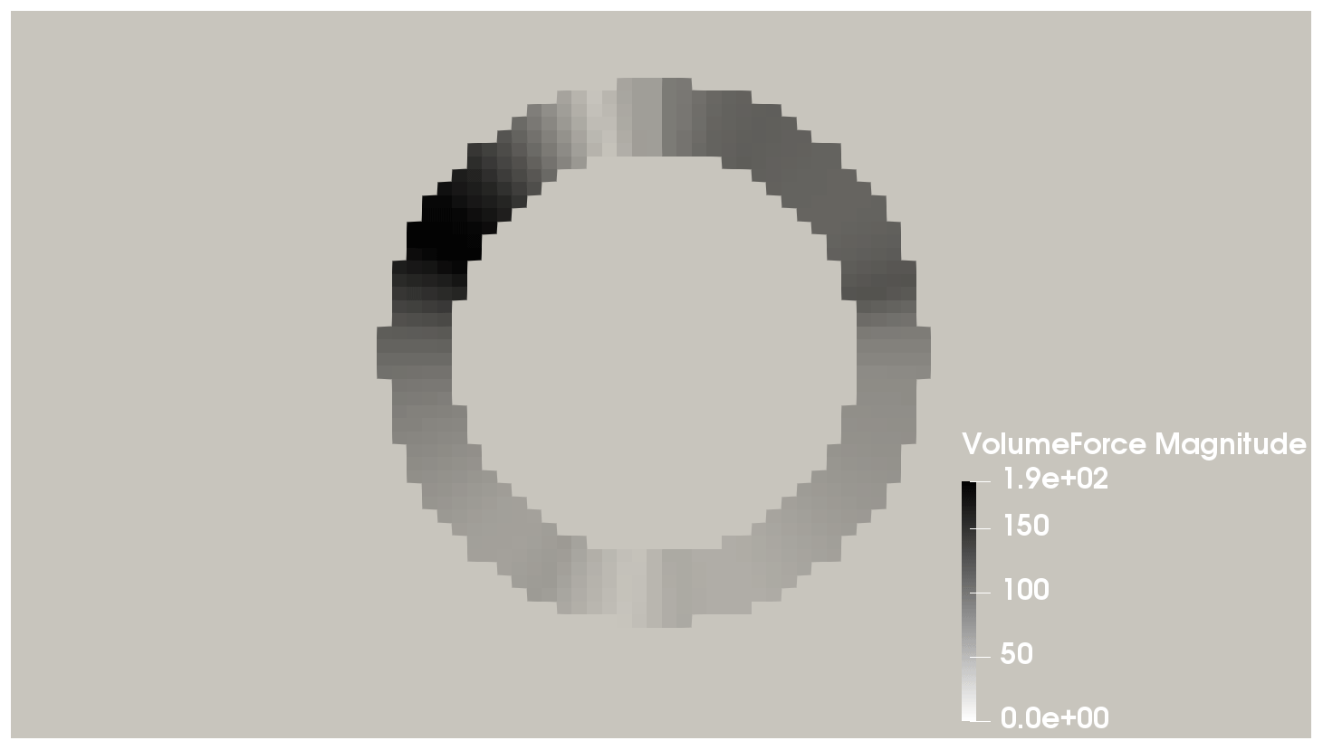
Figure 5Volumetric forces acting on the cylinder. Flow goes from left to right. Free stream speed is 8 m s−1, with a coarse mesh.
This section is meant to test the capabilities of the RANS-AC in a multi-turbine environment. Experimental data from a small wind farm of VAWTs were found in Araya et al. (2014). These kinds of experiments are hard to find in the literature since most experimental studies on VAWTs are done on one turbine only. The experiment consists of a set of turbines that can be rearranged in any fashion in order to test the performance of several layouts; the location is in the Antelope Valley, California. The turbines are the same 1.2 kW Windspire turbines mentioned in the past sections. Although data for multiple wind-turbine arrays are available, only data from two different arrays will be used here, namely an array of four turbines and another array of 18 turbines. Figures 6 and 7 show the layouts of the two arrays. The 18-turbine array has counterclockwise-rotating turbines. It is said in Araya et al. (2014) that the most prevalent wind direction is from the southwest; therefore the turbines in Figs. 6 and 7 were aligned in that direction. The wind speed is about 8 m s−1 and λ is kept at 2.3. The value of I is set to 0.13 according to Table 2.
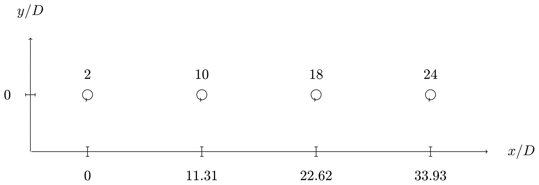
Figure 6Four turbines in a row. The distance from turbine to turbine is 11.31 D (diameters). Flow is from left to right.
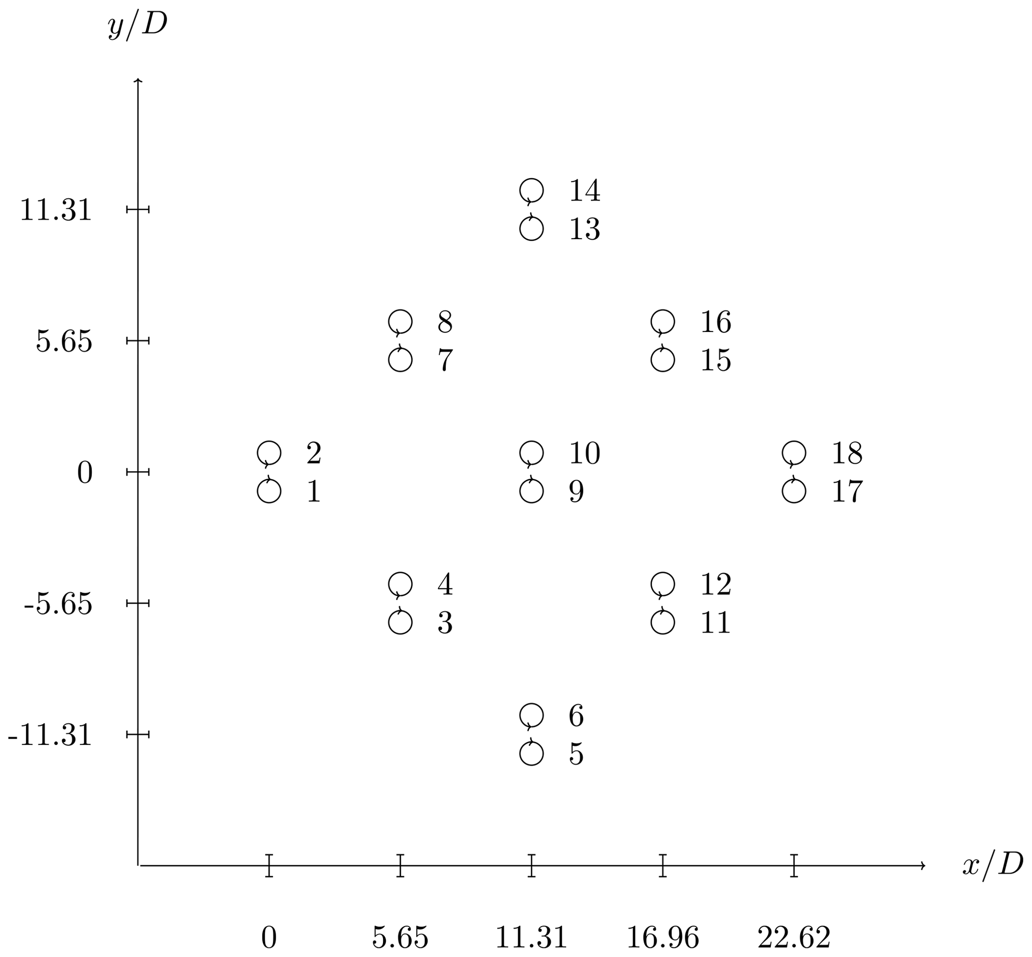
Figure 7Fish schooling configuration. Turbines are placed in a counterclockwise-rotating fashion. The flow is also from left to right.
3.1 Model calibration
Since the numerical simulation must be provided with the turbulence length scale in order to compute the turbulent kinetic energy dissipation rate at the inlet, a study on the width of the wake was conducted in order to find the appropriate turbulence length scale. The results in Table 1 were obtained supposing that the width of the wake was similar to the diameter of the turbines. This did not impact the results of the CP; however, it was observed that the streamwise development of the wake was sensitive to this value – this is reflected in ϵ since it depends on l=0.08L, where L is the width of the wake.
In order to obtain a value for l, a simulation with L=D was run and the width of the wake was found. Care must be taken in selecting the width of the wake as it varies downstream. It was decided to take the value at 7 D, roughly; the reason for this is that the rate of growth begins to reach a steady value. The rate of growth of the wake at small distances downwind cannot be neglected. At larger distances the wake begins to fade away and a wake width is hard to define. This is exemplified in Fig. 8; the procedure consisted in placing several downwind stations, e.g., crosswind plots of the magnitude of the velocity. The width was then measured from end to end, where each end has a velocity value of the free stream velocity, which is 8 m s−1 in this case. These ends can be found visually by intersecting the wake plot with a horizontal line drawn at U=8 m s−1, where U is the magnitude of the velocity. Notice in the figure that the location at which the ends of the wake stop varying is at 7 D approximately. The width is then , where y+ is the upper end and y− is the lower end. It is also interesting to notice the skewness of the wake, since the turbine is rotating counterclockwise; most of the power is extracted in the positive portion of y.
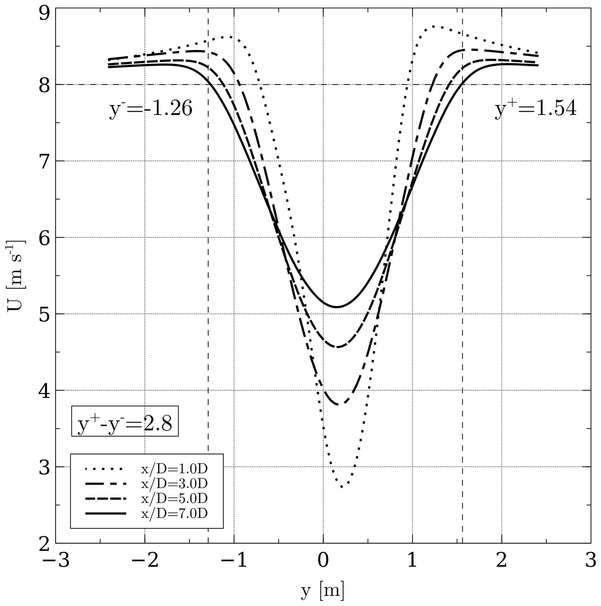
Figure 8Wake width at different downwind stations. The width begins to reach a stable value at 7 D, and its value is 2.8 m.
Once the new value of L was found, an iterative procedure following the same logic was conducted: a new simulation with L=2.8 was conducted, and the width of the wake was obtained in the same fashion. The procedure was stopped when the width stops varying across iterations. Figure 9 shows the final value of the width of the wake, which is 3.7 m; the turbulence length scale is found by substituting 3.7 in l=0.08L.
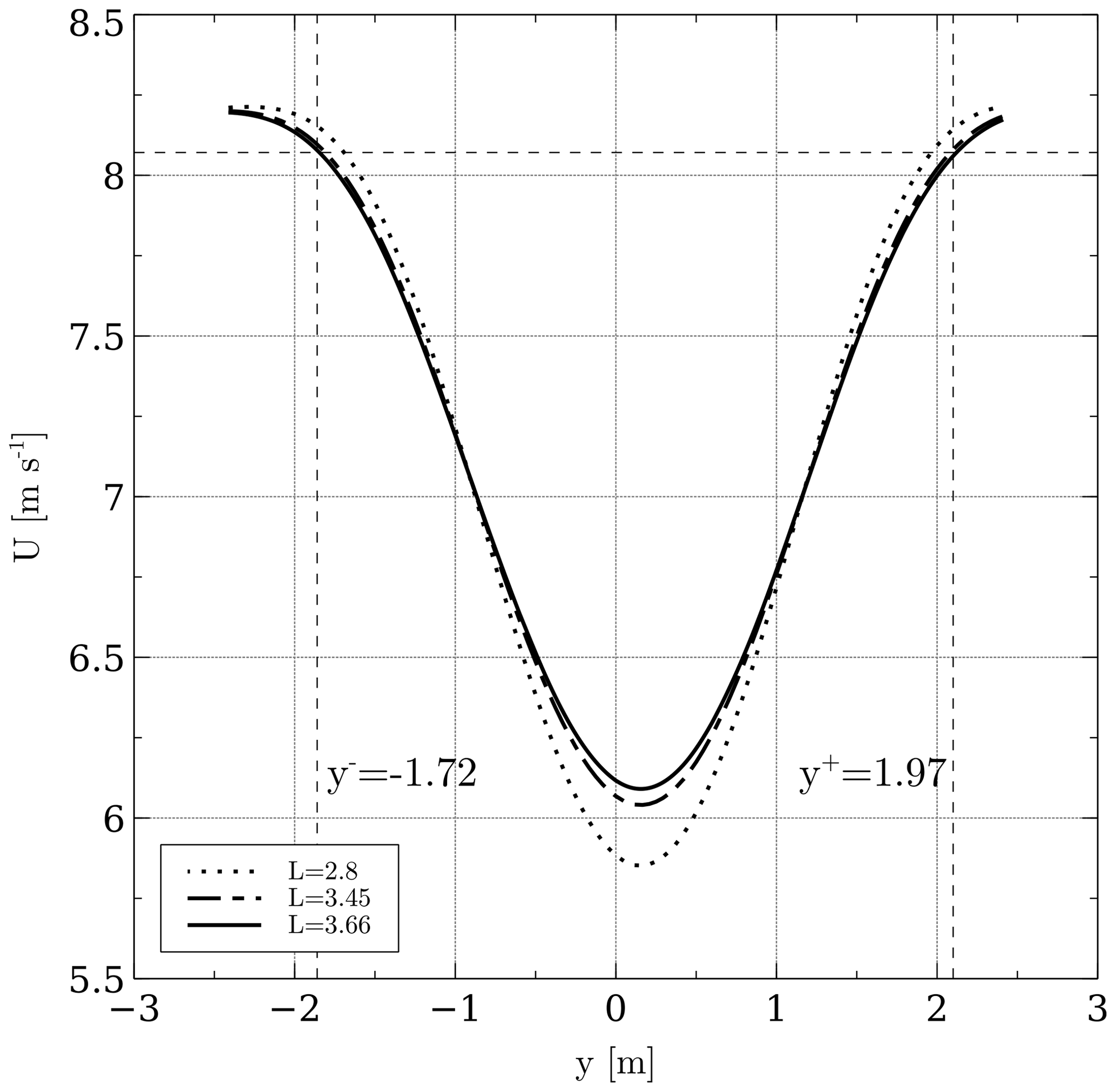
Figure 9Wake widths obtained by following an iterative procedure. All the plots are located at 7 D downwind.
3.2 Array of four turbines
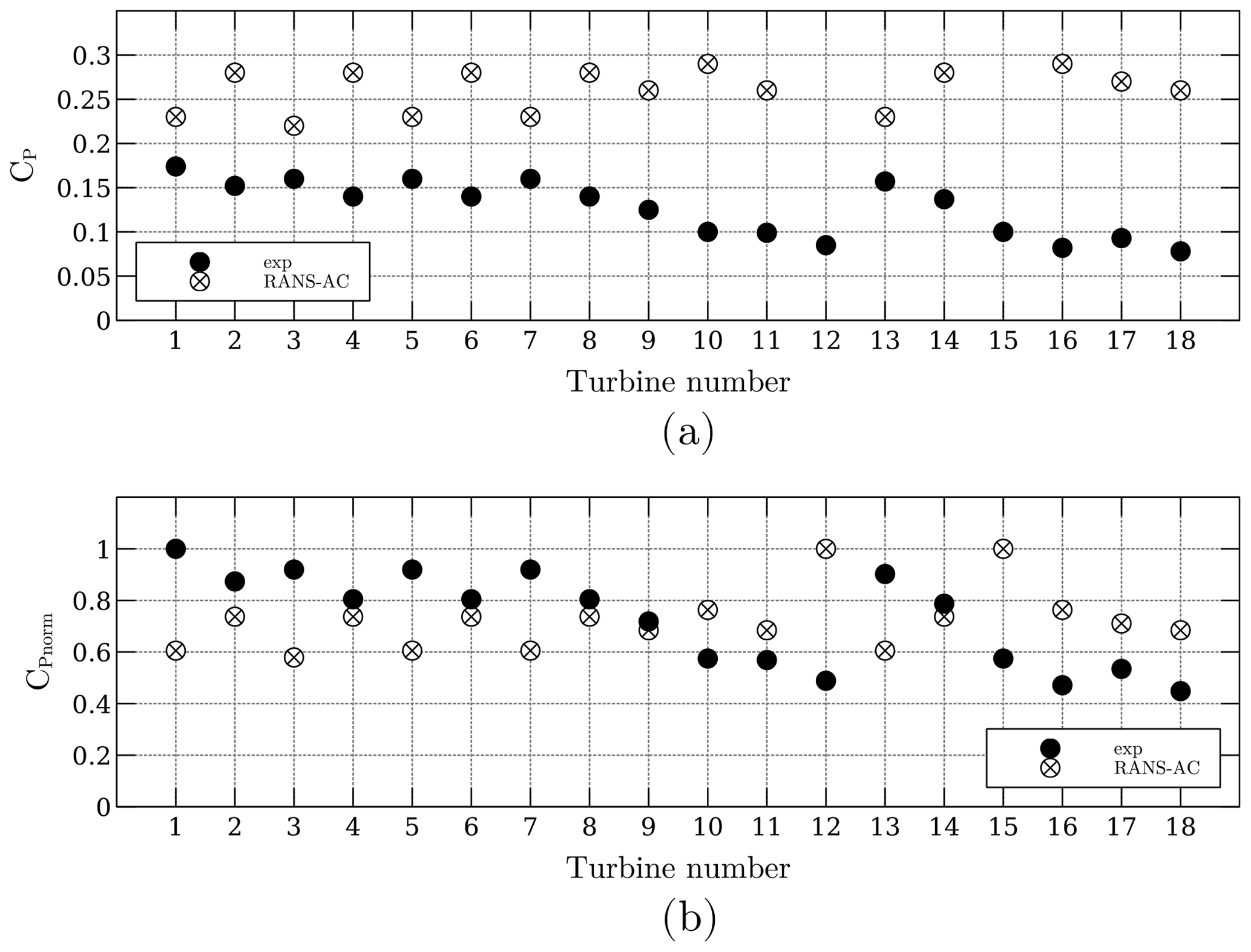
The power coefficients from this array were obtained from data published by Araya et al. (2014). The script used to extract information from the data set is presented in Appendix B. The distance from turbine to turbine is 11.31 D. Figure 10 shows the CP and the normalized CP. The latter was taken to be the current turbine CP divided by the leading turbine CP; experimental data were normalized with the leading turbine's experimental CP, and numerical data were normalized accordingly. There is a clear overestimation of the CP; as discussed earlier, the AC model tended to overestimate the CP of this particular turbine. The normalized CP shows that there is an overall good trend: the power coefficients decrease in the same manner.
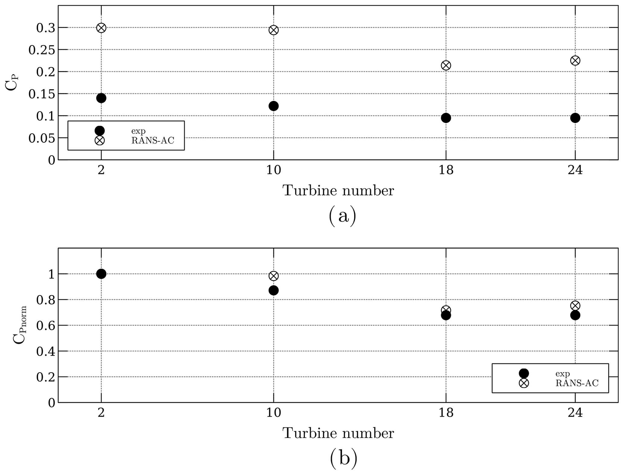
Figure 10Power coefficients of the four-turbine array. Panel (a) is the actual CP, and panel (b) is the normalized CP.
Another plot concerning the velocity and turbulence intensity along the center line is included in Fig. 11. The magnitude of the velocity is normalized with respect to the free stream velocity U∞. The value of I was calculated in Paraview by creating a new field according to the following equation derived from Eq. (20).
The RANS-AC underestimates the wake recovery in between the turbines. The value of I starts at 0.13 according to Table 2, and then it reaches a steady pattern past the second turbine; values up to 0.4 can be found near the wake of each turbine.
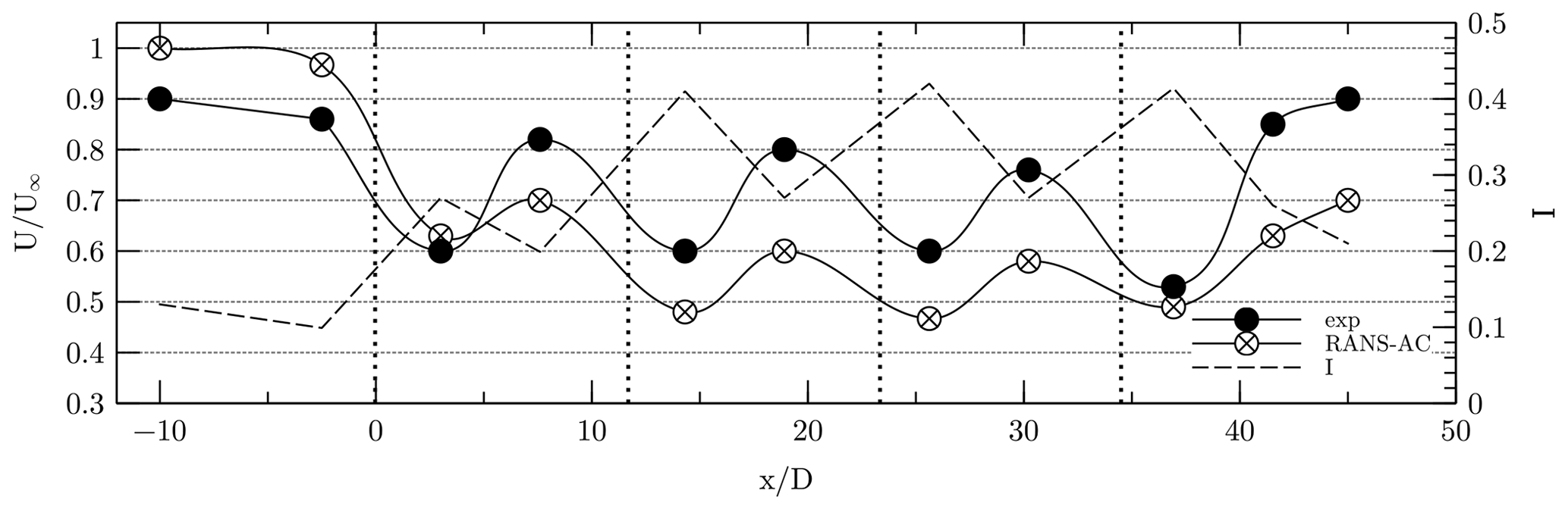
Figure 11Wake across the turbine array. The axis for I is located at the right side of the plot. Vertical dotted lines signify the locations of each turbine.
3.3 Array of 18 turbines
A plot similar to Fig. 10 is presented for this case. Unfortunately, the CP's across the array do not follow a coherent pattern; e.g., turbines that have been blocked present similar or even higher CP's than the turbines free of blockage. Figure 12 shows the current CP in panel (a) and the normalized CP in panel (b). The normalized CP was obtained by dividing each CP by the maximum CP.
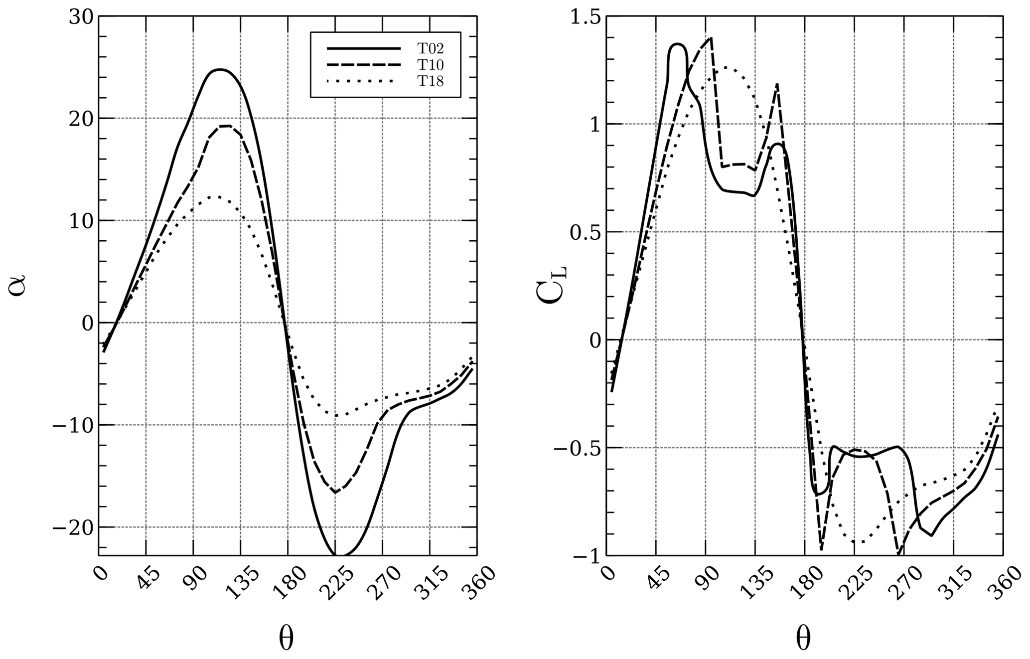
It was observed that a portion of the angles of attack of the turbines that were free of blockage were above stall according to Fig. 2. This is wrong since the manufacturer states that the turbine is kept at an optimal λ of 2.3, therefore meaning that it is not stalled. As the flow traverses each turbine downwind, it loses momentum; therefore each blocked turbine sees lower relative velocities and thus lower angles of attack. It would be intuitive to think that lower angles of attack lead to lower lift coefficients, but since the turbine is stalled, the lift coefficients might be even higher than those in the stalled regime. Data extracted from a row of turbines in the array are presented in Fig. 13. The plot shows the angles of attack and lift coefficients from turbines 2, 10 and 18. It can be seen that there is indeed a decrease in the amplitude of α as each turbine presents blockage from another turbine; however, it is important to notice that, in this case, turbine 18, for instance, has the lowest amplitude of α, but its coefficients are not in the stall region where they drop sharply, therefore achieving higher lift and tangential force coefficients. The local Re ranges from 100 000 to 200 000, and the positive stall angle of attack is about 16∘ according to Fig. 2. Turbine 18 has a maximum positive α of 13∘; therefore it operates at an optimal regime, which should not happen actually.
It must be clear that this fault is due to the wrong predictions of α in the AC model, which is possible in case high-solidity turbines are being used. The incoherent pattern of CP's along a row of turbines did not occur in the case of the array of four turbines. It is thought that this array was not affected by the accelerated flow in between turbines as in the case of the array of 18 turbines; therefore the velocity across the center line decayed faster and the turbines in the back rows operated in a regime well below stall, achieving even lower CP's.
As seen in Sect. 3, the case of the 18-turbine wind farm did not yield good results mainly because of the inability of the AC model to correctly predict angles of attack for high-solidity turbines. In seeing this, an additional verification study was done to prove that the RANS-AC does work well indeed if low-solidity turbines are used. The work from Shamsoddin and Porté-Agel (2016) is used as a reference. An LES simulation was carried out on a three-bladed VAWT with a radius of 25 m, a chord of 1.5 m and a height of 100 m. The wing's cross section is an NACA0018. The rotational speed is 16.5 rpm, and the wind speed is 9.6 m s−1, thus yielding a tip-speed ratio of 4.5. The turbulence intensity value at the inlet is 0.083, and an atmospheric boundary layer is used, although this is not possible in a 2D simulation. Figure 14 shows a CP plot against λ. The current RANS simulation was done a cylinder thickness of two chords and an enclosing square of 30×30 cells. Although the RANS-AC model overpredicts the value of CP, there is a very good agreement on the trend of the curve. Results from the stand-alone AC model are presented too.

Figure 14Comparison of CP results from an LES simulation with the current RANS-AC. The turbine's σ is 0.09.
Next, a comparison of the wake of the turbine is presented. The LES wake is taken at the Equator. The width of the wake L was taken as the diameter of the turbine, and the iterative procedure shown in Sect. 3 was not done since the results using the diameter as the width of the wake were satisfactory. The accurate width of the wake seemed to impact mostly the initial value of ϵ (which depends on l=0.08L) at the inlet, and not much difference was observed in the wake recovery when using the diameter as the width of the wake. Figure 15 shows very good agreement in the development of the wake.
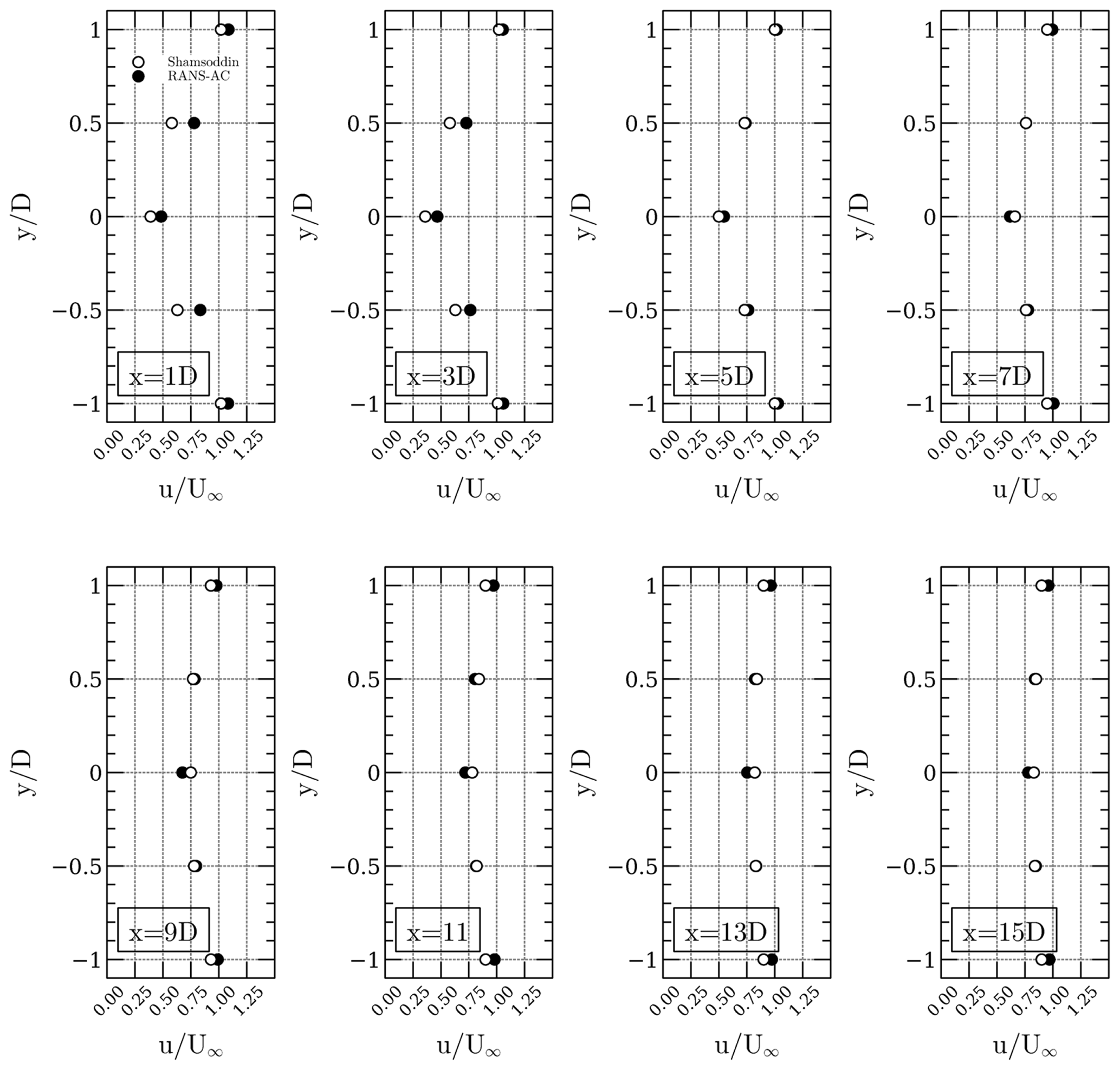
Figure 15Comparison of the LES wake at different downwind distances with the current RANS-AC results.
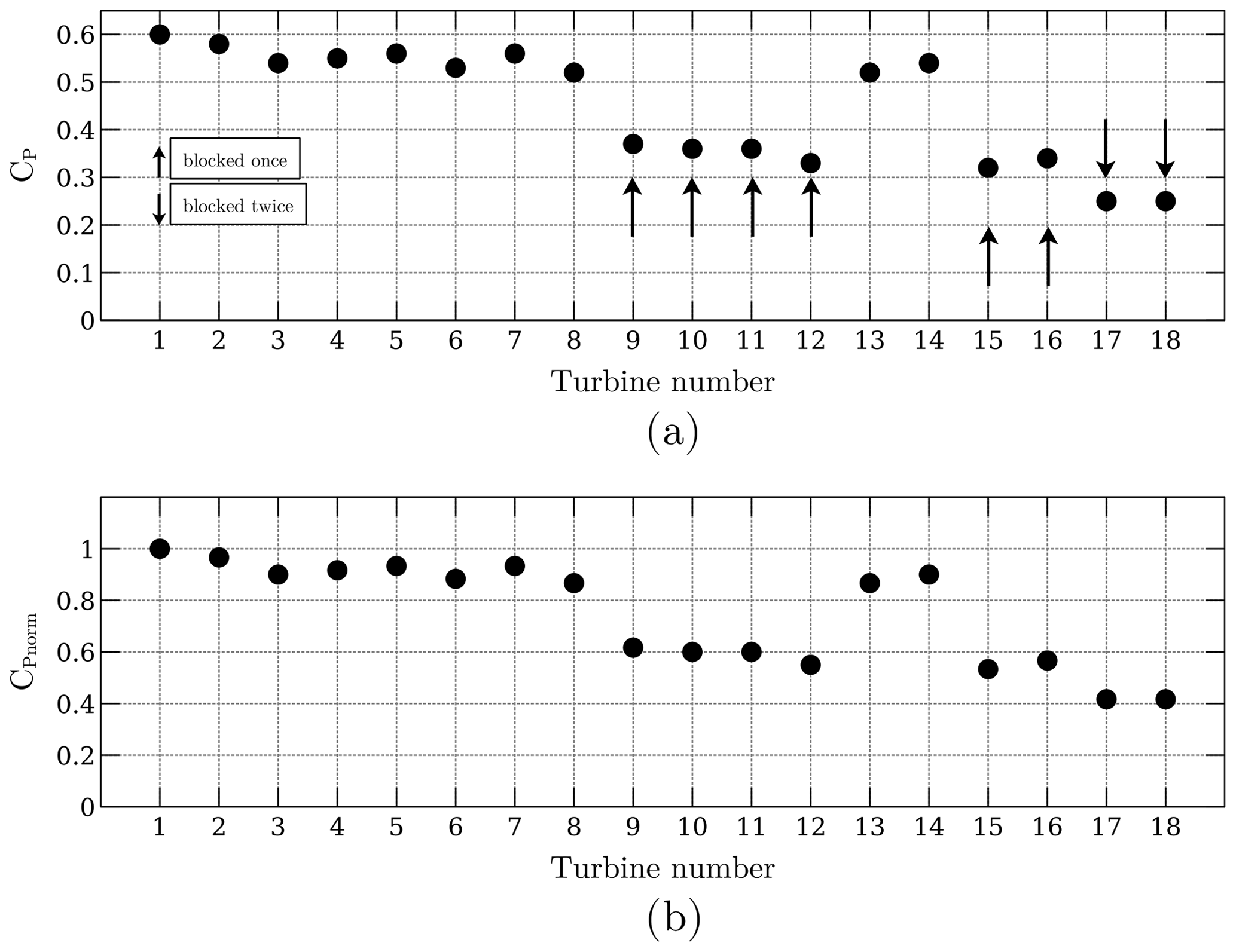
Figure 16Wind farm array of 18 turbines using the 25 m radius turbine from Shamsoddin and Porté-Agel (2016). Panel (a) shows the current CP, and panel (b) shows the normalized CP. Arrows pointing upwards denote turbines that are blocked by only one turbine, whereas arrows that point downwards denote turbines that have been blocked by two turbines.
Finally, the same 18-turbine wind farm simulation is done, except this time the turbine from Shamsoddin and Porté-Agel (2016) is used. The relative distances from turbine to turbine are preserved. The Reynolds number could not be preserved because that would imply running the turbine at extremely low wind speeds and extremely low rpm. The purpose is to show that the RANS-AC has no trouble predicting the right trend of the power coefficients when using low-solidity turbines. The solver converged at 1564 iterations, although the power coefficients reached an almost constant value at 1000 iterations. Roughly an hour had passed by the time the solver reached 1000 iterations; this was done on an all-in-one computer using only one 2.5 GHz processor and 12 GB RAM. The distance from the last turbine to the outlet was half the distance from the first turbine to the last turbine, or . Larger distances yielded the same results. It must be mentioned that it is not necessary to resolve the entire wake of the turbines until they recover the free stream value; this is possible thanks to the velocity outlet boundary condition, which is zeroGradient. Figure 16 shows the power coefficients and the normalized power coefficients. The normalized coefficients were calculated by dividing all CP's by the maximum CP. A coherent pattern is observed: the higher the blockage, the lower the CP value is. Also, the CP's of the turbines free of blockage were notably higher than those of the plot in Fig. 14; a maximum of 0.59 was found in one of the leading turbines, whereas a single isolated turbine had a CP of 0.49. It is believed that the accelerated flow in some regions impacts the CP's, and thus different values are obtained as if they were isolated.
The RANS-AC was successfully implemented in OpenFOAM. This was confirmed by the fact that it could achieve a power coefficient very similar to the stand-alone AC. Guidelines for selecting the mesh size and the thickness of the actuator were also given along with inlet boundary conditions for the RANS simulation. The model was validated against multi-turbine experiments, and good agreement was found concerning the trend of the power coefficients in a row of four VAWTs. Unfortunately these multi-turbine experiments were done using small turbines which had a high solidity; this caused the model to wrongly predict the angles of attack, namely overestimating the angles of attack and thus getting the wrong coefficients of lift and tangential force. Thus results from the array of 18 turbines could not match the experimental data. An additional verification against a large VAWT LES simulation (Shamsoddin and Porté-Agel, 2016) with a low solidity was conducted to prove that the RANS-AC is indeed capable of model the wind farm power coefficients so long as the leading turbines were not incorrectly predicted in the stall regime by the AC. The comparison with the results of the wake of the large VAWT was in very good agreement. Although a multiple-turbine simulation was not done in Shamsoddin and Porté-Agel (2016), a simulation of an array of 18 turbines preserving the original relative distances between turbines in Araya et al. (2014) was conducted. This time, the RANS-AC predicted a coherent pattern of the power coefficients across the array; e.g., the turbines free of blockage had higher power coefficients, and the turbines that experienced more blockage from other turbines had lower power coefficients. The RANS-AC can therefore be used to model entire wind farms provided low-solidity turbines are used. Future work will consider wind farm optimizations with this model along with artificial intelligence to predict the performance of a particular wind farm in different locations. A neural network can be used to learn to predict the power coefficients of a farm depending the wind velocity and wind direction. This farm could then predict its own performance when seeing different wind speeds and directions. Choosing the right array for a particular location can potentially impact the rate of return of a wind farm project.
import pandas as pd
df = pd.read_csv(path, skiprows=5)
df.head

data = df.iloc[:, [7, 8]]
data.columns = ['avg', 'std']

# I at 4 m/s
df4 = data[(data.avg > 3) & (data.avg < 5)]
print( (df4['std'] / df4['avg']).mean() )

# I at 6 m/s
df6 = data[(data.avg > 5) & (data.avg < 7)]
print( (df6['std'] / df6['avg']).mean() )

# I at 8 m/s
df8 = data[(data.avg > 7) & (data.avg < 9)]
print( (df8['std'] / df6['avg']).mean() )

# I at 10 m/s
df10 = data[(data.avg > 9) & (data.avg < 11)]
print( (df10['std'] / df10['avg']).mean() )

# I at 12 m/s
df12 = data[(data.avg > 11) & (data.avg < 13)]
print( (df12['std'] / df12['avg']).mean() )

# I at 14 m/s
df14 = data[(data.avg > 13) & (data.avg < 15)]
print( (df14['std'] / df14['avg']).mean() )
import pandas as pd
df = pd.read_csv(path, skiprows=5)
df.head

data = df.iloc[:, [2, 4, 7, 11]]
data.columns = ['n', 'p', 'u', 'd']

cp_02 = data[ (data['n'] == 2) &
((data['u'] > 7.5) & (data['u'] < 8.5)) &
((data['d'] > 210) & (data['d'] < 235)) ]['p'].mean()

cp_10 = data[ (data['n'] == 10) &
((data['u'] > 7.5) & (data['u'] < 8.5)) &
((data['d'] > 210) & (data['d'] < 235)) ]['p'].mean()

cp_18 = data[ (data['n'] == 18) &
((data['u'] > 7.5) & (data['u'] < 8.5)) &
((data['d'] > 210) & (data['d'] < 235)) ]['p'].mean()

cp_24 = data[ (data['n'] == 24) &
((data['u'] > 7.5) & (data['u'] < 8.5)) &
((data['d'] > 210) & (data['d'] < 235)) ]['p'].mean()

H = 6.1
D = 1.2
A = H * D
U = 8
RHO = 1.15
pinf = (1 / 2) * RHO * (U ** 3) * A

cp_02 /= pinf 		# cp of turbine 02
cp_10 /= pinf 		# cp of turbine 10
cp_18 /= pinf 		# cp of turbine 18
cp_24 /= pinf 		# cp of turbine 24
Codes are available at https://doi.org/10.5281/zenodo.5177216 (Martinez-Ojeda, 2021a).
Data sets are available at https://doi.org/10.5281/zenodo.5177214 (Martinez-Ojeda, 2021b).
This video explains the results of the 18-large-turbine wind farm. Pressure and velocity fields are shown (https://www.youtube.com/watch?v=Q6qZG6-oC3A, last access: 10 August 2021) (Martinez-Ojeda, 2021c).
The supplement related to this article is available online at: https://doi.org/10.5194/wes-6-1061-2021-supplement.
EMO was the main author of this work; he developed the stand-alone actuator-cylinder code and the actuatorCylinderSimpleFoam solver for OpenFOAM. MS contributed to the guidance, suggestions and some of the writing in LaTeX as well as some figures. FJSO contributed to the guidance, suggestions and revision of this work.
The authors declare that they have no conflict of interest.
Publisher's note: Copernicus Publications remains neutral with regard to jurisdictional claims in published maps and institutional affiliations.
The main author of this work would like to thank CONACYT (Consejo Nacional de Ciencia y Tecnología) as well as the OpenFOAM community.
This paper was edited by Alessandro Bianchini and reviewed by two anonymous referees.
Abkar, M.: Impact of Subgrid-Scale Modeling in Actuator-Line Based Large-Eddy Simulation of Vertical-Axis Wind Turbine Wakes, Atmosphere, 9, 257, https://doi.org/10.3390/atmos9070257, 2018. a
Abkar, M.: Theoretical Modeling of Vertical-Axis Wind Turbine Wakes, Energies, 12, 10, https://doi.org/10.3390/en12010010, 2019. a
Araya, D., Craig, A., Kinzel, M., and Dabiri, J.: Low-order modeling of wind farm aerodynamics using leaky Rankine bodies, J. Renew. Sustain. Energ., 6, 063118-1–063118-20, https://doi.org/10.1063/1.4905127, 2014. a, b, c, d, e, f
Bachant, P., Goude, P., and Wosnik, M.: Actuator line modeling of vertical-axis turbines, Physics – Fluid Dynamics, Center for Ocean Renewable Energy, University of New Hampshire, Durham, NH, USA, 2018. a
Bardina, J., Huang, P., and Coakley, T.: Turbulence Modeling Validation, Testing, and Development, Tech. rep., National Aeronautics and Space Administration, Ames Research Center, National Technical Information Service, https://doi.org/10.2514/6.1997-2121, 1997. a
Bremseth, J. and Duraisamy, K.: Computational analysis of vertical axis wind turbine arrays, Theor. Comput. Fluid Dynam., 30, 387–401, 2016. a
Cheng, Z.: Integrated dynamic analysis of floating vertical axis wind turbines, PhD thesis, Norwegian University of Science and Technology, Faculty of Engineering Science and Technology, Department of Marine Technology, Trondheim, Norway, 2016. a, b, c
Cheng, Z., Madsen, H. A., Gao, Z., and Moan, T.: Aerodynamic Modeling of Floating Vertical Axis Wind Turbines Using the Actuator Cylinder Flow Method, Energ. Proced., 94, 531–543, https://doi.org/10.1016/j.egypro.2016.09.232, 2016. a
Claessens, M.: The Design and Testing of Airfoils for Application in Small Vertical Axis Wind Turbines, MS thesis, TU Delft, Delft, the Netherlands, 2006. a, b
Drela, M.: XFOIL: An Analysis and Design System for Low Reynolds Number Airfoils, Low Reynolds Number Aerodynamics, in: Lecture Notes in Engineering, vol. 54, Springer, Berlin, Heidelberg, 1989. a
Giorgetti, S., Pellegrini, G., and Zanforlin, S.: CFD investigation of the aerodynamics interferences between medium solidity Darrieus vertical axis wind turbines, Energ. Proced., 81, 227–239, https://doi.org/10.1016/j.egypro.2015.12.089, 2015. a
Hansen, J. T., Mahak, M., and Tzanakis, I.: Numerical modelling and optimization of vertical axis wind turbine pairs: A scale up approach, Renew. Energy, 171, 1371–1381, https://doi.org/10.1016/j.renene.2021.03.001, 2021. a
Hezaveh, S., Bou-Zeid, E., Dabiri, J., Kinzel, M., Cortina, G., and Martinelli, L.: Increasing the Power Production of Vertical-Axis Wind-Turbine Farms Using Synergistic Clustering, Bound.-Lay. Meteorol., 9, 275–296, https://doi.org/10.1007/s10546-018-0368-0, 2018. a
Jensen, N.: A Note on Wind Turbine Interaction, Technical Report Ris-M-2411, Roskilde National Laboratory, Roskilde, Denmark, 1983. a
Li, A.: Double actuator cylinder model of a tandem vertical-axis wind turbine counter-rotating rotor concept operating in different wind conditions, MS thesis, Technical University of Denmark, Department of Wind Energy, Roskilde, Denmark, 2017. a, b, c, d, e, f
Madsen, H.: The actuator cylinder: a flow model for vertical-axis wind turbines, PhD thesis, Aalborg University Centre, Aalborg, 1982. a, b
Madsen, H., Larsen, T., Vita, L., and Paulsen, U.: Implementation of the actuator cylinder flow model in the hawc2 code for aeroelastic simulations on vertical axis wind turbines, in: chap. 913, 51st AIAA Aerospace Sciences Meeting including the New Horizons Forum and Aerospace Exposition, Grapevine, Dallas/Ft. Worth Region, Texas, 2013. a, b
Marten, D., Wendler, J., Pechlivanoglou, G., Nayeri, C., and Paschereit, C.: Qblade: An Open Source Tool for Design and Simulation of Horizontal and Vertical Axis Wind Turbines, Int. J. Emerg. Technol. Adv. Eng., 3, 264–269, 2013. a
Martinez-Ojeda, E.: EdgarAMO/actuatorCylinderSimpleFoam-solver: actuatorCylinderSimpleFoam-solver (v1.0.0), Zenodo [code], https://doi.org/10.5281/zenodo.5177216, 2021a. a
Martinez-Ojeda, E.: EdgarAMO/actuatorCylinderSimpleFoam-data: actuatorCylinderSimpleFoam-data (v1.0.0), Zenodo [data set], https://doi.org/10.5281/zenodo.5177214, 2021a. a
Martinez-Ojeda, E.: actuatorCylinderSimpleFoam results in paraview, available at: https://www.youtube.com/watch?v=Q6qZG6-oC3A, last access: 10 August 2021. a
Mendoza, V. and Goude, A.: Wake flow simulation of a vertical-axis wind turbine under the influence of wind shear, J. Phys., 854, 012031, https://doi.org/10.1088/1742-6596/854/1/012031, 2017. a
Migliore, P. G., Wolfe, W. P., and Fanucci, J. B.: Flow Curvature Effects on Darrieus Turbine Blade Aerodynamics, J. Energy, 4, 79-0112R, https://doi.org/10.2514/3.62459, 1980. a, b, c, d
Moukalled, F., Mangani, L., and Darwish, M.: The finite volume method in computational fluid dynamics an advanced introduction with OpenFOAM and Matlab, 1st Edn., Springer International Publishing, Switzerland, 2016. a
Ning, A.: Actuator cylinder theory for multiple vertical axis wind turbines, Wind Energ. Sci., 1, 327–340, https://doi.org/10.5194/wes-1-327-2016, 2016. a, b, c, d
Paraschivoiu, I.: Wind turbine design with emphasis on Darrieus concept, Presses Internationales Polytechnique, Quebec, Canada, 2002. a, b
Shamsoddin, S. and Porté-Agel, F.: A Large-Eddy Simulation Study of Vertical Axis Wind Turbine Wakes in the Atmospheric Boundary Layer, Energies, 9, 366, https://doi.org/10.3390/en9050366, 2016. a, b, c, d, e, f
Sheldahl, R. and Klimas, P.: Aerodynamic Characteristics of Seven Symmetrical Airfoil Sections Through 180-Degree Angle of Attack for Use in Aerodynamic Analysis of Vertical Axis Wind Turbines, Tech. Rep. SAND80-2114, Sandia National Laboratories, Albuquerque, NM, USA, 1981. a
Svenning, E.: Implementation of an actuator disk in OpenFOAM, Tech. rep., Chalmers University of Technology, Gothenburg, Sweden, 2010. a
Versteeg, H. and Malalasekera, W.: An Introduction to Computational Fluid Dynamics, Prentince Hall, New York, 1995. a
Whittlesey, R. W., Liska, S., and Dabiri, J. O.: Fish schooling as a basis for vertical axis wind turbine farm design, Bioinspirat. Biomimet., 5, 035005, https://doi.org/10.1088/1748-3182/5/3/035005, 2010. a
Wilcox, D.: Turbulence Modeling for CFD, 2nd Edn.,DCW Industries, Anaheim, 1998. a
Zanforlin, S. and Nishino, T.: Fluid dynamics mechanisms of enhanced power generation by closely-spaced vertical axis wind turbines, Renew. Energy, 99, 1213–1226, https://doi.org/10.1016/j.renene.2016.08.015, 2016. a, b
- Abstract
- Introduction
- Actuator-cylinder (AC) wake model for turbines
- Validation against Araya et al. (2014)
- Verification with Shamsoddin and Porté-Agel (2016)
- Conclusions
- Appendix A: Turbulence intensity data script
- Appendix B: Power coefficients data script
- Code availability
- Data availability
- Video supplement
- Author contributions
- Competing interests
- Disclaimer
- Acknowledgements
- Review statement
- References
- Supplement