Probabilistic estimation of the Dynamic Wake Meandering model parameters using SpinnerLidar-derived wake characteristics

We study the calibration of the Dynamic Wake Meandering (DWM) model using high-spatial- and high-temporal-resolution SpinnerLidar measurements of the wake field collected at the Scaled Wind Farm Technology (SWiFT) facility located in Lubbock, Texas, USA. We derive two-dimensional wake flow characteristics including wake deficit, wake turbulence, and wake meandering from the lidar observations under different atmospheric stability conditions, inflow wind speeds, and downstream distances up to five rotor diameters. We then apply Bayesian inference to obtain a probabilistic calibration of the DWM model, where the resulting joint distribution of parameters allows for both model implementation and uncertainty assessment. We validate the resulting fully resolved wake field predictions against the lidar measurements and discuss the most critical sources of uncertainty. The results indicate that the DWM model can accurately predict the mean wind velocity and turbulence fields in the far-wake region beyond four rotor diameters as long as properly calibrated parameters are used, and wake meandering time series are accurately replicated. We show that the current DWM model parameters in the IEC standard lead to conservative wake deficit predictions for ambient turbulence intensities above 12 % at the SWiFT site. Finally, we provide practical recommendations for reliable calibration procedures.

1 Introduction

Wake effects are perceived as one of the largest sources of uncertainty in energy production and load estimates of onshore and offshore wind farms (Walker et al., 2016). Within an iterative design process and/or optimization study, wake effects on aeroelastic turbine responses are predicted using engineering wake models, e.g. the Dynamic Wake Meandering (DWM) (Madsen et al., 2010) and Frandsen (Frandsen, 2007) models, which can be used within simple and fast design tools (Braunbehrens and Segalini, 2019). Their main limitation is their reduced ability to fully resolve the turbulence structures of the wake field, which often leads to an inaccurate representation of the flow field and biased power and load predictions (Reinwardt et al., 2018). To minimize the modelling uncertainty, it is a common practice to calibrate engineering wake models using field measurements when available or using higher-fidelity simulations like computational fluid dynamics (CFD).

Wind lidars have become popular for studying wind turbine wakes due to their higher spatial resolution and ease of installation compared to traditional anemometers mounted on meteorological masts (Machefaux et al., 2016). The use of lidar measurements to calibrate low-order wake models has already been successfully adopted (Trabucchi et al., 2017; Reinwardt et al., 2020; Zhan et al., 2020a). Although high-quality lidar observations of the wake field are available (Käsler et al., 2010; Iungo et al., 2013; Aitken et al., 2014), the spatial and temporal resolution required to characterize wake deficit, wake turbulence, and meandering characteristics is rarely achieved. Such resolution is a key characteristic for the development and evaluation of dynamic wake models.

The Scaled Wind Farm Technology (SWiFT) experiment, conducted at Sandia National Laboratories between 2016 and 2017 (Herges et al., 2017, 2018; Herges and Keyantuo, 2019), provides a fairly complete and suitable dataset for the calibration and evaluation of wake models (Doubrawa et al., 2019, 2020; Conti et al., 2020a). The SWiFT dataset consists of concurrent measurements of inflow conditions from a heavily instrumented meteorological mast, high-spatial- and high-temporal-resolution measurements of a single wake flow field behind a turbine from a nacelle-mounted SpinnerLidar, and power and load measurements from a second turbine operating in the waked field. The detailed instrumentation of the site allows the investigation of the wake field variability under different atmospheric-stability conditions as well as the analysis of the wake-induced effects on the waked-turbine operation (i.e. power and load predictions).

Here, we analyse the SWiFT dataset aiming at calibrating and evaluating the DWM model. This model is recommended in the IEC 61400-1 standard (IEC, 2019) for the purpose of wind turbine and wind farm design certification, and it is widely used in load assessments under wake conditions (Larsen et al., 2013; Galinos et al., 2016; Reinwardt et al., 2018, 2020; Dimitrov, 2019). The DWM model simulates wind field time series and is divided into three parts: a wake deficit component, which simulates the velocity deficit; a wake-added turbulence component; and a wake meandering component, which is a stochastic meandering process. These three components are presumed to affect wind turbine loading conditions (Keck et al., 2012; Galinos et al., 2016; Larsen et al., 2013; Dimitrov, 2019). Although several studies have demonstrated the superior performance of the DWM model compared to other engineering wake models that only predict steady wake features (Thomsen et al., 2007; Larsen et al., 2013; Reinwardt et al., 2018), the accuracy of both the DWM-simulated wake flow fields and the resultant turbine power and load predictions is still to be assessed.

1.1 A review of the DWM model

The underlying hypothesis of the DWM model is to consider the wake as a passive tracer of the large incoming turbulence structures. The so-called split-in-scales assumption (Larsen et al., 2008) states that the large-scale turbulent eddies contained in the atmospheric boundary layer are the main drivers of the wake meandering, whereas the smaller turbulent eddies govern the wake deficit evolution downstream of the rotor. Further, wake deficits from upstream turbines are transported in the streamwise direction, assuming Taylor's hypothesis of frozen turbulence (Larsen et al., 2015). This set of assumptions allows for the decoupling of the wake deficit and wake-added turbulence formulations from the wake meandering process (Larsen et al., 2007). Therefore, the three components of the DWM model can be computed separately and successively superimposed on turbulence fields to generate wake time series, which can be used as inputs to aeroelastic simulations (Larsen et al., 2013; Keck et al., 2014a).

The wake deficit formulation of the DWM model is mainly based on the work of Ainslie (1987) and solves the axisymmetric Navier–Stokes (N–S) equations with an eddy viscosity term and a set of calibration parameters. Initially, the DWM model was calibrated with CFD simulations performed by Madsen et al. (2010). Keck et al. (2012) derived a two-dimensional model of the eddy viscosity term and updated the calibration parameters based on CFD simulations. Larsen et al. (2013) found that the calibration parameters of the former two studies were not suitable for predicting power and loads at the Egmond aan Zee offshore wind farm. To match the measured power, they introduced an artificial filtering function in the eddy viscosity term and re-calibrated the deficit model; however, this calibration was not based on the spatial description of the wake flow field but on power production data. The eddy viscosity model to predict velocity deficits in the current IEC standard (IEC, 2019) is inspired by the work of Larsen et al. (2013).

Keck et al. (2014a, 2015) proposed a correction factor to the eddy viscosity term, which includes the effects of atmospheric stability and shear on the turbulence mixing occurring in the wake, and re-calibrated the model parameters. Although these improvements were verified against large-eddy simulations (LESs), the influence of atmospheric stability on the wake deficit evolution was hardly observed during a lidar campaign (Machefaux et al., 2016; Larsen et al., 2015), in which it was argued that atmospheric stability affects to a large extent the meandering process. A load validation study using the DWM model with calibrated parameters from both Madsen et al. (2010) and Keck et al. (2012) as well as the IEC standard (IEC, 2019) was conducted by Reinwardt et al. (2018), who collected load measurements at the ECN wind turbine test site in Germany and at the Technical University of Denmark (DTU) test site in Høvsøre in Denmark. They found fatigue load biases within the range of 11 %–15 % for the tower bottom and 8 %–21 % for the blade-root flapwise bending moments. Reinwardt et al. (2020) derived a new set of calibration parameters based on full-field lidar observations of the wake field from a wind farm in the south-east of Hamburg, Germany. They demonstrated that improved wake deficit predictions can be obtained by calibrating the DWM model with nacelle-mounted lidars.

The fidelity of the simulated wake meandering dynamics also affects the accuracy of load predictions (Larsen et al., 2013; Conti et al., 2021). Modelling of the meandering process relies on a suitable stochastic turbulence field and definition of the large-scale turbulence structures. Larsen et al. (2008) and Trujillo et al. (2011) demonstrated that the large-scale eddies can be extracted from the incoming atmospheric turbulence field from local mast measurements. Alternatively, the wake meandering process can be simulated through synthetic wind fields generated using stochastic turbulence models (i.e. the turbulence model by Mann, 1994) and a definition of the large-scale eddies or by means of LESs. Machefaux et al. (2015) showed that inconsistencies between a Mann-based and LES-based meandering process can arise due to differences in the input turbulence fields. Larsen et al. (2008) and Trujillo et al. (2011) defined the large-scale eddies on the order of two rotor diameters (D) or larger as responsible for wake meandering, whereas other studies defined scales larger than 3–4 D as dominant (Espana et al., 2011; Muller et al., 2015; Yang and Sotiropoulos, 2019). Despite the severe impact of the wake meandering dynamics on load predictions, its uncertainty has not been assessed in load validation studies due to lack of data (Larsen et al., 2013; Churchfield et al., 2015; Reinwardt et al., 2018). However, aeroelastic simulations with constrained wake meandering dynamics can potentially decrease the uncertainty in load predictions under wake conditions (Conti et al., 2021).

Further, the added turbulence formulation in the DWM model accounts for additional mechanically generated turbulence caused by the wake shear and the breakdown of tip and root vortices. These contributions are modelled by a semi-empirical formulation that uses parameters, which were calibrated against CFD simulations (Madsen et al., 2010). To our knowledge, no further development has been made on this subject.

1.2 Problem statement

As described above, there is no consensus for the values of the DWM model parameters when studying load predictions at any given site. Also, and perhaps most importantly, we do not know the sources of uncertainty observed in previous studies that used the model (Larsen et al., 2013; Churchfield et al., 2015; Reinwardt et al., 2018), which need to be addressed to provide reliable load predictions. The common practice has been to derive optimized sets of model parameters based on limited synthetic or experimental data. This has led to an unknown confidence in the overall model prediction ability; incorrect calibration of the model parameters may impact significantly the model performance and lead to suboptimal wind turbine designs.

To address this issue, we estimate uncertainties in the calibration parameters of the DWM model by applying Bayesian inference (Box and Tiao, 1973), which consists of updating any related prior information on model parameters by incorporating new knowledge obtained from wake flow characteristics derived through lidar measurements. Further, the Bayesian calibration provides a systematic approach to include various types of uncertainty such as physical variability as well as measurement and modelling errors. This paper focuses on improving and validating the calibration of DWM model parameters using lidar-derived wake features and has a fourfold primary purpose:

1. Derive wake flow features such as the two-dimensional velocity deficit and wake-added turbulence profiles as well as time series of the wake meandering in both lateral and vertical directions from the SpinnerLidar measurements under different inflow wind speeds and atmospheric-stability conditions.

2. Calibrate the DWM-model-based wake deficit and wake-added turbulence predictions using the SpinnerLidar-derived wake flow features and the Bayesian inference framework.

3. Propagate modelling uncertainties in fully resolved wake flow fields for robust predictions that take into account the calibrated uncertainties.

4. Conduct a sensitivity analysis to determine the most significant sources of uncertainty in simulated wake fields that are typically inputs to aeroelastic simulations.

This study contributes to the ongoing discussion regarding the accuracy of power and load predictions of wind turbines operating under wake situations (Conti et al., 2020b, 2021) by quantifying uncertainties in wake simulations performed with the DWM model under a variety of inflow wind conditions. The outcomes of this study are useful for improving currently adopted wake simulation procedures for load analysis in the IEC standards as well as to provide practical recommendations for wake model calibration studies based on measurements from nacelle-mounted lidars.

The work is organized as follows. Section 2 describes the DWM model. The SWiFT layout and relative wind site conditions are described in Sect. 3. In Sect. 4, we present the wind field retrieval assumptions used to derive wake features from SpinnerLidar measurements. The Bayesian calibration of the DWM model is performed in Sect. 5. We carry out the validation of the wind turbine wake simulations and conduct a sensitivity analysis to investigate the most influential parameters in Sect. 6. Finally, the last two sections are dedicated to the discussions and conclusions.

2 Dynamic Wake Meandering model

The DWM model resolves three main wake features: the quasi-steady velocity deficit, the wake-added turbulence, and the wake meandering. Each model component is described separately in the following subsections.

2.1 Quasi-steady velocity deficit

The quasi-steady velocity deficit component describes the wake expansion and recovery caused partly by the recovery of the rotor pressure field and partly by turbulence diffusion moving farther downstream of the rotor (Larsen et al., 2013). The wake deficit is formulated in the meandering frame of reference (MFoR), which is a coordinate system with origin in the centre of symmetry of the deficit.

In the far-wake region, i.e. distances larger than two rotor diameters (Sanderse, 2015), the deficit evolution is assumed to be governed by turbulent mixing and is described by the thin shear layer approximation of the rotational symmetric N–S equations with the pressure term disregarded (Madsen et al., 2010). To account for the neglected pressure gradient effects, an initial wake deficit is analytically formulated based on the turbine's axial induction derived from blade element momentum (BEM) theory (Madsen et al., 2010). The turbulence closure of the N–S equations is obtained by means of an eddy viscosity term, and the momentum equation is solved numerically using a finite difference scheme with the artificial initial deficit as a boundary condition (Madsen et al., 2010). Here, we use the numerical scheme of the stand-alone DWM model (Liew et al., 2020; Larsen et al., 2020). We refer to the generalized definition of the non-dimensional eddy viscosity term by Keck et al. (2012), who considered two major drivers to the turbulence mixing: the ambient turbulence (TI_amb) and turbulence induced by the wake shear layer:

$$\begin{array}{}\text{(1)}& \begin{array}{rl}& {\displaystyle \frac{{\mathit{\nu }}_{\mathrm{T}}}{U_{\mathrm{amb}}R}}(r,\stackrel{\mathrm{̃}}{x})=F_{\mathrm{1}}\left(\stackrel{\mathrm{̃}}{x}\right)k_{\mathrm{1}}{\mathrm{TI}}_{\mathrm{amb}}+F_{\mathrm{2}}\left(\stackrel{\mathrm{̃}}{x}\right)k_{\mathrm{2}}max\\ & \left({\displaystyle \frac{R_{\mathrm{w}}(\stackrel{\mathrm{̃}}{x}{)}^{\mathrm{2}}}{U_{\mathrm{amb}}R}}\left|{\displaystyle \frac{\partial U(\stackrel{\mathrm{̃}}{x},r)}{\partial r}}\right|;{\displaystyle \frac{R_{\mathrm{w}}\left(\stackrel{\mathrm{̃}}{x}\right)}{R}}\left(\mathrm{1}-{\displaystyle \frac{U_{\min }}{U_{\mathrm{amb}}}}\right)\right),\end{array}\end{array}$$

where ν_T is the eddy viscosity, U_amb is the ambient wind speed at hub height, and R is the rotor radius. The first term on the right-hand side of Eq. (1) describes the contribution of the ambient turbulence and the second the self-generated turbulence by the wake shear layer. Madsen et al. (2010) proposed the wake radius $R_{\mathrm{w}}\left(\stackrel{\mathrm{̃}}{x}\right)$, where $\stackrel{\mathrm{̃}}{x}$ is the downstream distance normalized by R, and the maximum velocity difference (U_amb−U_min), where U_min is the minimum wind speed in the wake, as the turbulent length and velocity scales, respectively, that govern turbulent mixing due to the wake shear layer.

Based on classical mixing length theory, Keck et al. (2012) defined the turbulence stresses to be proportional to the local velocity gradient $\partial U(\stackrel{\mathrm{̃}}{x},r)/\partial r$, which provides a two-dimensional eddy viscosity formulation that is a function of the axial and radial coordinates, $\stackrel{\mathrm{̃}}{x}$ and r, respectively. The max operator is included to avoid underestimating the turbulent stresses at locations where the velocity gradient of the deficit approaches zero. Both terms in Eq. (1) include a filter function ($F_{\mathrm{1}}\left(\stackrel{\mathrm{̃}}{x}\right)$ and $F_{\mathrm{2}}\left(\stackrel{\mathrm{̃}}{x}\right)$) and a model constant (k₁ and k₂). The filter functions are required to model the turbulence development behind the rotor and have values in the range of 0–1, depending on the downstream distance only (Keck et al., 2012). F₁ accounts for the delay of the ambient turbulence entrainment into the wake and is assumed to “activate” ambient turbulence effects at downstream distances where the pressure has recovered (i.e. 2 D downstream, where the far wake begins; Sanderse, 2015).

F₂ compensates for the initial non-equilibrium between the mean velocity field and the turbulent energy content created due to the rapid change in mean flow gradients close to the rotor. We refer to Eqs. (17) and (18) in Keck et al. (2015) for the mathematical formulation of F₁ and F₂; k₁ and k₂ are calibration parameters that govern the turbulence mixing and presumably do not change with wind turbine design and ambient conditions (Keck et al., 2012).

2.2 Wake turbulence

The wake turbulence is composed of three turbulence sources and can be defined as follows (Vermeer et al., 2003):

$$\begin{array}{}\text{(2)}& {\mathrm{TI}}_{\mathrm{wake}}=\sqrt{{\mathrm{TI}}_{\mathrm{amb}}^{\mathrm{2}}+{\mathrm{TI}}_{\mathrm{m}}^{\mathrm{2}}+{\mathrm{TI}}_{\mathrm{add}}^{\mathrm{2}}},\end{array}$$

where TI_m denotes the turbulence induced by the meandering of the wake deficit, and TI_add is the wake-added turbulence. TI_m is commonly denoted as the apparent turbulence (Madsen et al., 2005) as the stochastic meandering of the wake deficit induces additional velocity fluctuations into time series taken at fixed locations in the wake. This term is considered the main source of added turbulence in the far wake (Madsen et al., 2010), while its spatial distribution can be computed by the convolution of the wake deficit in the MFoR and the probability distribution function (PDF) of the wake meandering in the lateral and vertical directions (Keck et al., 2014a). TI_add accounts for the shear- and mechanically generated turbulence due to blade tip and root trailing vortices. The inhomogeneity of the wake-added turbulence is modelled by scaling the local turbulence using the factor k_mt (Madsen et al., 2010) as

$$\begin{array}{}\text{(3)}& k_{\mathrm{mt}}\left(r\right)=\mid \mathrm{1}-U_{\mathrm{def},\mathrm{MFoR}}\left(r\right)\mid k_{\mathrm{m}\mathrm{1}}+\left|{\displaystyle \frac{\partial U_{\mathrm{def},\mathrm{MFoR}}\left(r\right)}{\partial r}}\right|k_{\mathrm{m}\mathrm{2}},\end{array}$$

where U_def, MFoR is the velocity deficit in the MFoR, and k_m1 and k_m2 are constants calibrated based on CFD results (Madsen et al., 2010). The wake-added turbulence derived from Eq. (3) is presumed to meander together with the wake deficit, thus being displaced by the large-scale eddies in the atmosphere.

2.3 Meandering model

Here, the meandering model is confined to a single wake scenario, whereas multiple wake dynamics are described in Machefaux (2015). The wake field is modelled by considering a cascade of consecutive wake deficits that are displaced by the large-scale lateral- and vertical-velocity fluctuations, i.e. the wake transport velocities (v_c and w_c), corresponding to the lateral (y) and the vertical axis (z), respectively. Adopting Taylor's hypothesis, the downstream advection of these deficits is assumed to be controlled by the mean wind speed of the ambient wind field. Larsen et al. (2008) estimated v_c and w_c by low-pass filtering of atmospheric turbulence fluctuations. They defined a filtering cut-off frequency $f_{\mathrm{cut},\mathrm{off}}=U_{\mathrm{amb}}/\left(\mathrm{2}D\right)$, thus excluding contributions from smaller eddies to the meandering dynamics. This assumption was verified using full-scale lidar-based measurements collected behind an operating turbine (Bingöl et al., 2010). The wake displacements are computed as

$$\begin{array}{}\text{(4)}& \begin{array}{rl}y(x,\stackrel{\mathrm{‾}}{t})& =v_{\mathrm{c}}\left(\stackrel{\mathrm{‾}}{t}\right)\stackrel{\mathrm{‾}}{t}\left(x\right)+h_{\mathrm{yaw}}(x,\stackrel{\mathrm{‾}}{t})\\ z(x,\stackrel{\mathrm{‾}}{t})& =w_{\mathrm{c}}\left(\stackrel{\mathrm{‾}}{t}\right)\stackrel{\mathrm{‾}}{t}\left(x\right)+h_{\mathrm{tilt}}(x,\stackrel{\mathrm{‾}}{t}),\end{array}\end{array}$$

where $\stackrel{\mathrm{‾}}{t}=x/U_{\mathrm{amb}}$ defines the time for an air particle to move from the rotor to the downstream distance in the wake region. An appropriate choice of the transport velocity of the wake advection lies between the ambient wind speed and the centre velocity of the wake deficit (Keck et al., 2014b; Machefaux et al., 2015). The contribution from the yaw misalignment, which can redirect wakes in the lateral direction, is accounted for by $h_{\mathrm{yaw}}(x,\stackrel{\mathrm{‾}}{t})=x\tan \left(\mathit{\theta }\right(\stackrel{\mathrm{‾}}{t}\left)\right)$, where $\mathit{\theta }\left(\stackrel{\mathrm{‾}}{t}\right)$ is the yaw offset at the specific time (Machefaux, 2015; Vollmer et al., 2016). The contribution of the rotor tilt is considered by $h_{\mathrm{tilt}}(x,\stackrel{\mathrm{‾}}{t})$ (Machefaux, 2015).

3 The SWiFT facility

The SWiFT facility is a research site located in Lubbock, Texas, operated by Sandia National Laboratories (Herges et al., 2017). The site includes three Vestas V27 wind turbines, two meteorological towers, and a SpinnerLidar (Peña et al., 2018) mounted on the nacelle of one of the turbines and looking backwards. The entire site is on a fibre optic data acquisition and control network that synchronizes recordings from masts, turbines, and the SpinnerLidar (Herges et al., 2017, 2018). The measurement campaign took place between 2016 and 2017 with the main objective of characterizing wake fields and investigating wake steering control strategies (Herges et al., 2017).

Figure 1 provides an overview of the test layout together with the notation used throughout the paper. In this study, we analyse data collected at the meteorological mast (METa1), the turbine (WTGa1), and the SpinnerLidar mounted on the nacelle of the WTGa1. The METa1 (hereafter referred to as the mast) is 60 m tall and instrumented with sonic anemometers at 10, 18, 32, 45, and 58 m, sampling at 100 Hz. Other instruments installed on the mast are reported in Herges et al. (2017). The mast is placed 2.5 D south of WTGa1 in compliance with the IEC standard guidelines (IEC, 2015, 2017). As southerly winds are prevalent at the site (see Fig. 1, right), this layout allows the retrieval of concurrent incoming wind conditions from METa1, wake measurements behind the WTGa1 performed by the SpinnerLidar, and power and load measurements on the waked WTGa2 installed 5 D downstream. The WTGa1 and WTGa2 are variable-speed and pitch-regulated turbines with a hub height of 32.1 m, D=27 m, a cut-in wind speed of 3 m/s, and a maximum power output of 192 kW reached at the rated wind speed of 12 m/s (Berg et al., 2014). The supervisory control and data acquisition (SCADA) is available for both turbines, providing records of the rotor speed, pitch and yaw angles, and power production, among other information, at 50 Hz.

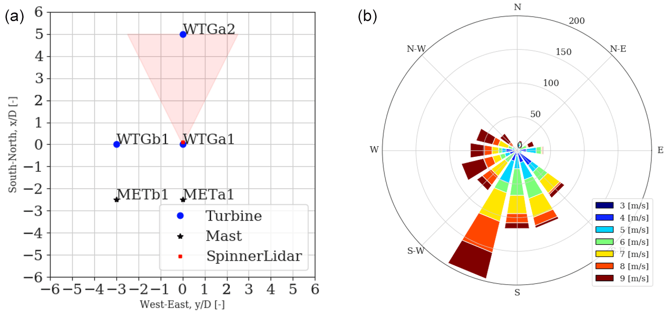
Figure 1 (a) A sketch of the SWiFT layout that includes locations of the main devices (i.e. wind turbines, masts, and the SpinnerLidar). The shaded red area indicates that the SpinnerLidar scans in the wake of WTGa1 assuming winds from the south. The distances are normalized with the rotor diameter D. (b) The wind rose at the site derived from the 32 m sonic observations collected on METa1 during the campaign.

3.1 SpinnerLidar

The SpinnerLidar is a research Doppler wind lidar developed at DTU based on a continuous-wave (CW) laser system (Peña et al., 2018). Hereafter, SpinnerLidar and lidar denote the same system. The SpinnerLidar has been mounted either in the spinner or on top of the nacelle of a wind turbine (Angelou and Sjöholm, 2015; Peña et al., 2018). In this study, the SpinnerLidar was installed on the nacelle of the WTGa1 and scanned the rotor wake at a high temporal and spatial resolution so that wake features could be derived. For the SWiFT campaign, the SpinnerLidar scanned continuously in a rose-pattern every 2 s (see Fig. 2), and the system internally subdivided the rose into 984 sections. The accumulated Doppler-shifted spectra at each of the sections was also recorded (Herges et al., 2017).

Once a scan was completed, the SpinnerLidar refocused at a different range, and this process took about 2 s (Herges et al., 2018). For the SWiFT campaign, several scanning strategies were adopted as described below.

• Strategy I. The SpinnerLidar scanned seven downstream distances: 1, 1.5, 2, 2.5, 3, 4, and 5 D. A full cycle (i.e. from 1 to 5 D) took 30–42 s. This dataset is suitable for investigating the wake deficit evolution and recovery behind the rotor; however, the frequency is too low to properly derive turbulence estimates or meandering dynamics.

• Strategy II. The SpinnerLidar scanned at the fixed distance of 2.5 D, ensuring both high spatial and temporal resolution; ≈298 rosette scans were generated within a 10 min period. This dataset is suited for turbulence and meandering investigations.

• Strategy III. The SpinnerLidar scanned at the fixed distance of 5 D behind the rotor, generating about 298 scans each 10 min. During this period, power and load measurements were recorded on WTGa2. This dataset is suitable for load validation analysis. Since it provides a description of the wake flow field, including velocity deficits, turbulence, and meandering at a distance that corresponds to typical spacings in wind farms, it is a valuable dataset for validating fully resolved wake flow predictions as long as induction effects are accounted for.

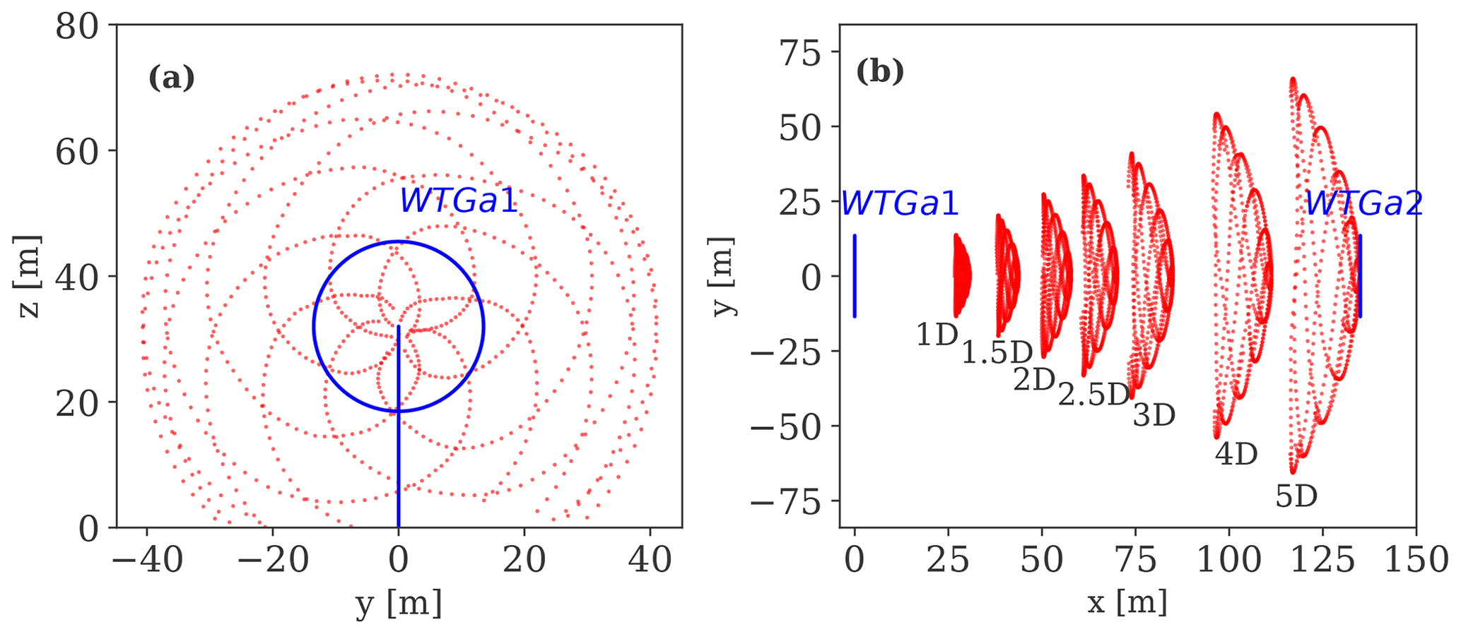
Figure 2 A schematic view of the SpinnerLidar's scanning pattern: (a) a front view at 2.5 D in the wake; (b) a top view including all scanned distances behind the WTGa1, which is depicted by solid blue lines. The WTGa2 is also shown.

3.2 Site conditions

For extended periods of the campaign, WTGa1 operated under large yaw misalignment as wake steering strategies were being investigated (Herges et al., 2017). To consider periods where WTGa1 is nearly aligned with the mean inflow, we filtered out 10 min periods characterized by an average yaw offset larger than $\pm \mathrm{10}{}^{\circ }$ compared to the free-stream wind direction (Conti et al., 2020a). The yaw offset is here defined as the difference between the nacelle orientation and the wind direction measured at the mast. Further, we focus the analysis on periods for which the free-stream wind direction is within 90–270^∘ (thus southern winds; see Fig. 1, right). This leads to about 850 available 10 min periods.

Figure 3 shows 10 min statistics of the hub-height turbulence intensity (TI_amb), the power-law shear exponent (α), and the power production of WTGa1 as a function of the hub-height mean wind speed (U_amb) based on the mast inflow measurements; α is computed from the sonic measurements at 18 and 45 m. As shown, the site is characterized by a wide range of turbulence and shear conditions, which are a consequence of the varying atmospheric stability (Doubrawa et al., 2019; Conti et al., 2020a). Further, relatively low wind speeds are recorded (3–10 m/s); thus WTGa1 operates below rated power, as seen in Fig. 3c. Because of this range of operating conditions, high rotor thrust coefficients that induce strong wake deficits characterize this dataset.

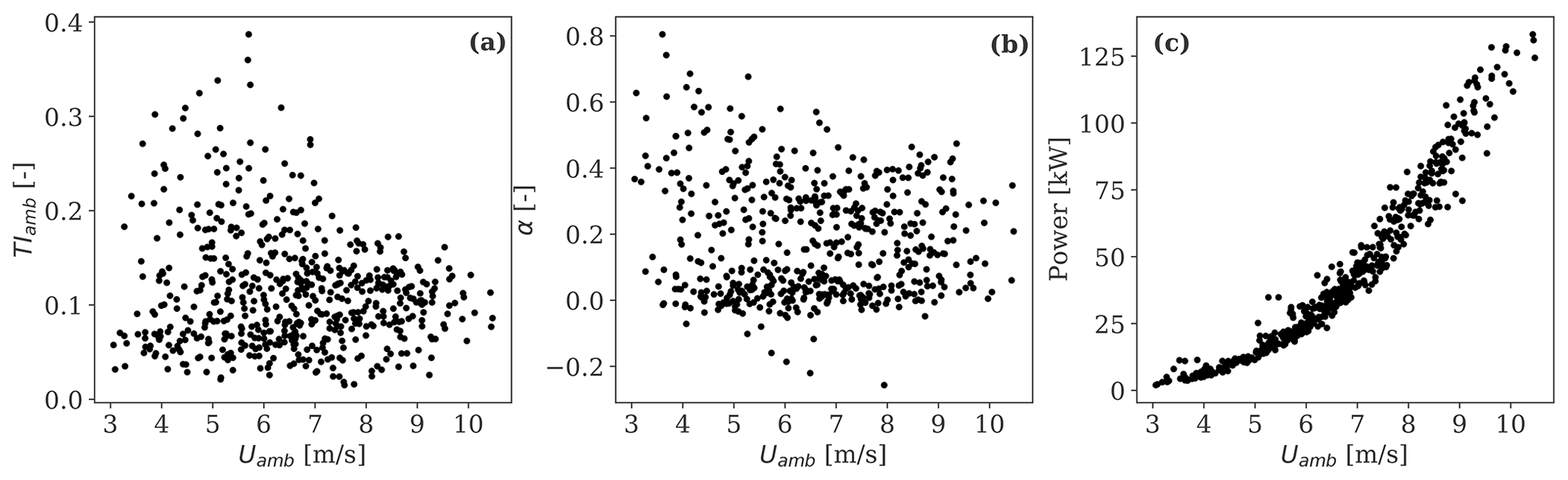
Figure 3 Inflow wind and operational conditions at the SWiFT site. (a) Hub-height turbulence intensity as a function of the hub-height mean wind speed based on the mast inflow measurements, (b) power-law shear exponent derived using observations from the 18 and 45 m sonic measurements, and (c) power productions of WTGa1 recorded from SCADA. Each marker represents a 10 min period.

3.2.1 Atmospheric stability

Here, we investigate the variability in the wake flow characteristics under varying stability and inflow wind speed conditions. We classify each 10 min sonically derived statistic into atmospheric-stability classes defined by ranges of the dimensionless stability parameter ($z/L$), where L is the Obukhov length (Monin and Obukhov, 1954) computed from the sonic measurements as

$$\begin{array}{}\text{(5)}& L=-{\displaystyle \frac{u_{*}^{\mathrm{3}}T}{kg\stackrel{\mathrm{‾}}{w{}^{\prime }{\mathrm{\Theta }}_{\mathrm{v}}{}^{\prime }}}},\end{array}$$

where $u_{*}=\sqrt{-\stackrel{\mathrm{‾}}{u^{\prime }{w}^{\prime }}}$ is the friction velocity, $\stackrel{\mathrm{‾}}{u^{\prime }{w}^{\prime }}$ is the local kinematic momentum flux, k=0.4 is the von Kármán constant, g is the acceleration due to gravity, T is the mean surface-layer temperature, the vertical velocity component is denoted by w, and Θ_v is the virtual potential temperature (which we approximate by the sonic temperature). The prime denotes fluctuations around the mean value, and the overbar is a time average. We define three main atmospheric-stability classes based on $z/L$ ranges by Peña (2019): unstable ($-\mathrm{2}<z/L<-\mathrm{0.2}$), near-neutral ($-\mathrm{0.2}<z/L<\mathrm{0.2}$), and stable ($\mathrm{0.2}<z/L<\mathrm{2}$) atmospheric conditions. We use the measurements at the 18 m sonic anemometer to derive the stability within each 10 min period. As shown in Conti et al. (2020a), the sonic measurements at 18 m provide the best fit to the polynomial form of Högström (1988), which describes the relation between the dimensionless wind shear ϕ_m and the dimensionless stability parameter $z/L$ in the surface layer (see middle panel of Fig. 3 in Conti et al., 2020a).

3.3 Data statistics

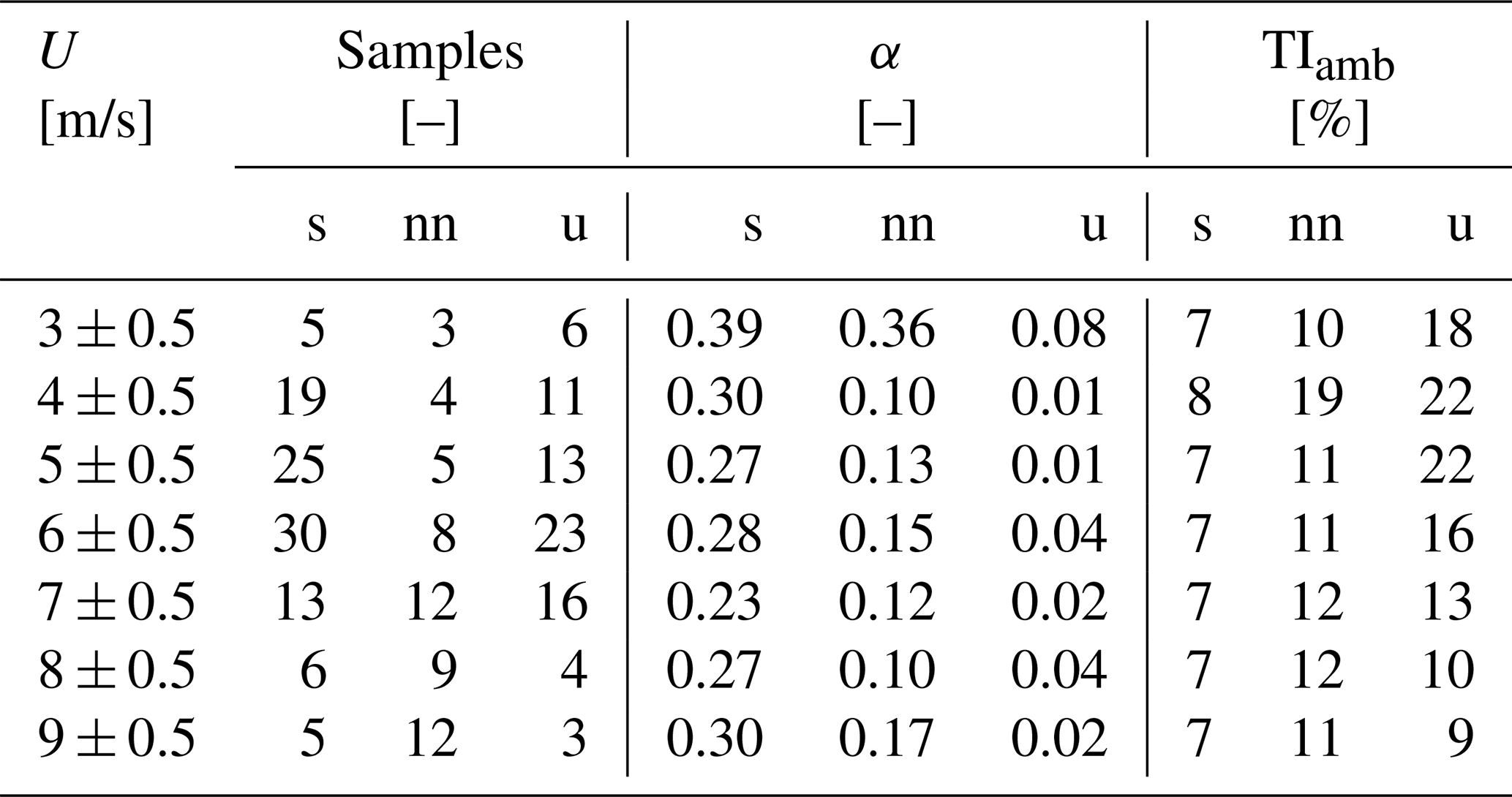
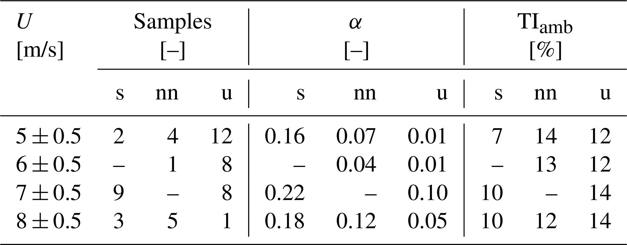
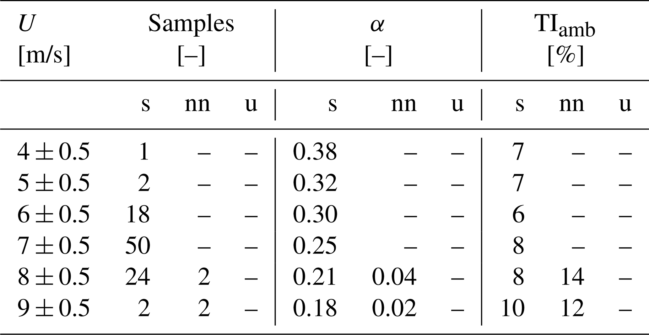
The statistics of the inflow wind parameters are presented separately in Tables 1, 2, and 3 according to the relative SpinnerLidar scanning strategy. Table 1 presents data collected during Strategy I. There is a fair number of 10 min periods to characterize the variability in the wake deficit with respect to atmospheric stability, inflow wind speeds, and downstream distances. The table shows increasing turbulence levels under unstable compared to stable cases, whereas relatively high vertical wind shears are found under stable conditions, as expected. The dataset is thus suitable for analysing the effects of atmospheric stability on the wake recovery. The dataset collected during Strategy II is reported in Table 2 and is used to characterize wake turbulence and meandering under different stability conditions. For Strategy III, represented in Table 3, the dataset is characterized by stable conditions mainly as the records correspond to night hours within three consecutive nights in July 2017.

Table 1 Dataset from Strategy I. The data are classified according to wind speed bins of 1 m/s and three atmospheric-stability classes: stable (s), near-neutral (nn), and unstable (u). The number of 10 min samples is also indicated; α is the power-law shear exponent; TI_amb is the turbulence intensity defined as the standard deviation of horizontal wind speed divided by the mean wind speed. The wind speed and turbulence parameters are obtained from sonic observations at 32 m height.

Table 2 Similar to Table 1 but for Strategy II.

Table 3 Similar to Table 1 but for Strategy III.

4 Lidar measurement processing

As lidars only measure the line-of-sight (LOS) velocity (v_los), assumptions are needed to reconstruct the three-dimensional wind field $\mathit{u}=(u,v,w)$, where u is the longitudinal, v the lateral, and w the vertical velocity component. If we neglect any probe volume averaging along the beam, v_los depends on the unit directional vector $\mathit{n}=(\cos \mathit{\varphi }\cos \mathit{\theta },\cos \mathit{\varphi }\sin \mathit{\theta },\sin \mathit{\varphi })$, which describes the scanning geometry through the elevation (ϕ) and azimuth (θ) angles and the wind field u,

$$\begin{array}{}\text{(6)}& v_{\mathrm{los}}(\mathit{\varphi },\mathit{\theta })=u\cos \left(\mathit{\varphi }\right)\cos \left(\mathit{\theta }\right)+v\cos \left(\mathit{\varphi }\right)\sin \left(\mathit{\theta }\right)+w\sin \left(\mathit{\varphi }\right).\end{array}$$

Considering the small elevation angles and the typical low values of w, we assume w=0 (Doubrawa et al., 2019, 2020). This assumption may introduce an error of up to 3 % in the reconstructed horizontal wind speed at short distances (1–2 D) (Debnath et al., 2019). Following the approach of Doubrawa et al. (2020), we can combine the u and v velocity components into a total horizontal wind vector, U, and Eq. (6) becomes

$$\begin{array}{}\text{(7)}& v_{\mathrm{los}}(\mathit{\varphi },\mathit{\theta },{\stackrel{\mathrm{‾}}{\mathit{\theta }}}_{\mathrm{0}})=U\cos \left(\mathit{\varphi }\right)\cos (\mathit{\theta }-{\stackrel{\mathrm{‾}}{\mathit{\theta }}}_{\mathrm{0}}),\end{array}$$

where ${\stackrel{\mathrm{‾}}{\mathit{\theta }}}_{\mathrm{0}}$ is the yaw offset, and the overbar indicates a smoothed signal as we apply a moving average operator with a 15 s window to the yaw misalignment to account for any temporal delay from the spatial distances among the mast, turbine's nacelle, and SpinnerLidar measurements (Conti et al., 2020a). With Eq. (7), we can reconstruct horizontal wind velocity measures at each individual scanned point within the rosette pattern. Further, we linearly interpolate the reconstructed wind speeds across the rosette pattern into a two-dimensional regular grid with a 2 m resolution, which is sufficient to characterize the spatial characteristics of the wind field in wakes (Fuertes et al., 2018; Conti et al., 2020a).

4.1 Lidar-estimated wake deficit

To perform comparisons with predicted velocity deficits from the DWM model, we aim at isolating the contribution of the wake deficit from that of the vertical wind shear in lidar measurements. As defined in Trujillo et al. (2011), the quasi-instantaneous wake deficit profile can be obtained by subtracting the mean vertical shear profile (U_amb(z)) from the quasi-instantaneous wake recording as

$$\begin{array}{}\text{(8)}& U_{\mathrm{def}}(x,y,z)={\displaystyle \frac{U_{\mathrm{amb}}\left(z\right)-U(x,y,z)}{U_{\mathrm{amb}}\left(z\right)}},\end{array}$$

where $U(x,y,z)$ is estimated from lidar measurements using Eq. (7), and U_amb(z) is the relative 10 min average inflow vertical wind speed profile measured at the mast. The deficit is then normalized with respect to the ambient wind speed profile. The v_los measurements and also the reconstructed U wind velocities are defined on a coordinate system that is attached either to the nacelle (nacelle frame of reference, NFoR), which rotates with the yawing of the turbine, or to the ground (fixed frame of reference, FFoR). To perform direct comparisons with the DWM model predictions, the lidar-estimated deficits obtained from Eq. (8) need to be computed in the MFoR. Here, this is performed by tracking the wake centre position through the method of Trujillo et al. (2011), where a bivariate Gaussian shape is fitted to the velocity deficit flow field, and the wake centre is the geometric centroid of the Gaussian function:

$$\begin{array}{}\text{(9)}& f_{\mathrm{def}}={\displaystyle \frac{A}{\mathrm{2}\mathit{\pi }{\mathit{\sigma }}_{\mathrm{w}y}{\mathit{\sigma }}_{\mathrm{w}z}}}\exp \left[-{\displaystyle \frac{\mathrm{1}}{\mathrm{2}}}\left({\displaystyle \frac{(y_i-{\mathit{\mu }}_y{)}^{\mathrm{2}}}{{\mathit{\sigma }}_{\mathrm{w}y}^{\mathrm{2}}}}+{\displaystyle \frac{(z_i-{\mathit{\mu }}_z{)}^{\mathrm{2}}}{{\mathit{\sigma }}_{\mathrm{w}z}^{\mathrm{2}}}}\right)\right],\end{array}$$

where μ_y and μ_z define the wake centre location; σ_wy and σ_wz are width parameters of the wake profile in the y and z directions, respectively; y_i and z_i denote the spatial locations of the lidar measurements; and A is a scaling parameter. Each scanned point of the quasi-instantaneous wake recording can be translated into the MFoR using the estimated μ_y and μ_z from Eq. (9) (Reinwardt et al., 2020). Therefore, we can compute the multiple wake recordings within a 10 min period in the MFoR and subsequently compute flow statistics such as the ensemble-average deficit profile as well as the spatial distribution of the wake turbulence in the MFoR. To ensure a high-quality fit, we reject scans where the estimated wake centre location is within ≈10 % of the lateral bounds of the scanning area and at more than 0.75 D from the hub height in the vertical direction (Doubrawa et al., 2020; Conti et al., 2020a).

Figure 4 illustrates ensemble-average measured deficit profiles in the MFoR at 2, 3, 4, and 5 D behind the rotor obtained from all 10 min periods characterized by an incoming wind speed of 7 m/s and under varying stability regimes during Strategy I (see Table 1 for reference). We can clearly observe the impact of the atmospheric stability and in particular of the associated turbulence levels on the wake recovery behind the rotor. A strong and well-defined symmetric wake deficit shape is seen under stable conditions (top row), whereas the deficits recover faster moving downstream as the atmosphere becomes more unstable (bottom row).

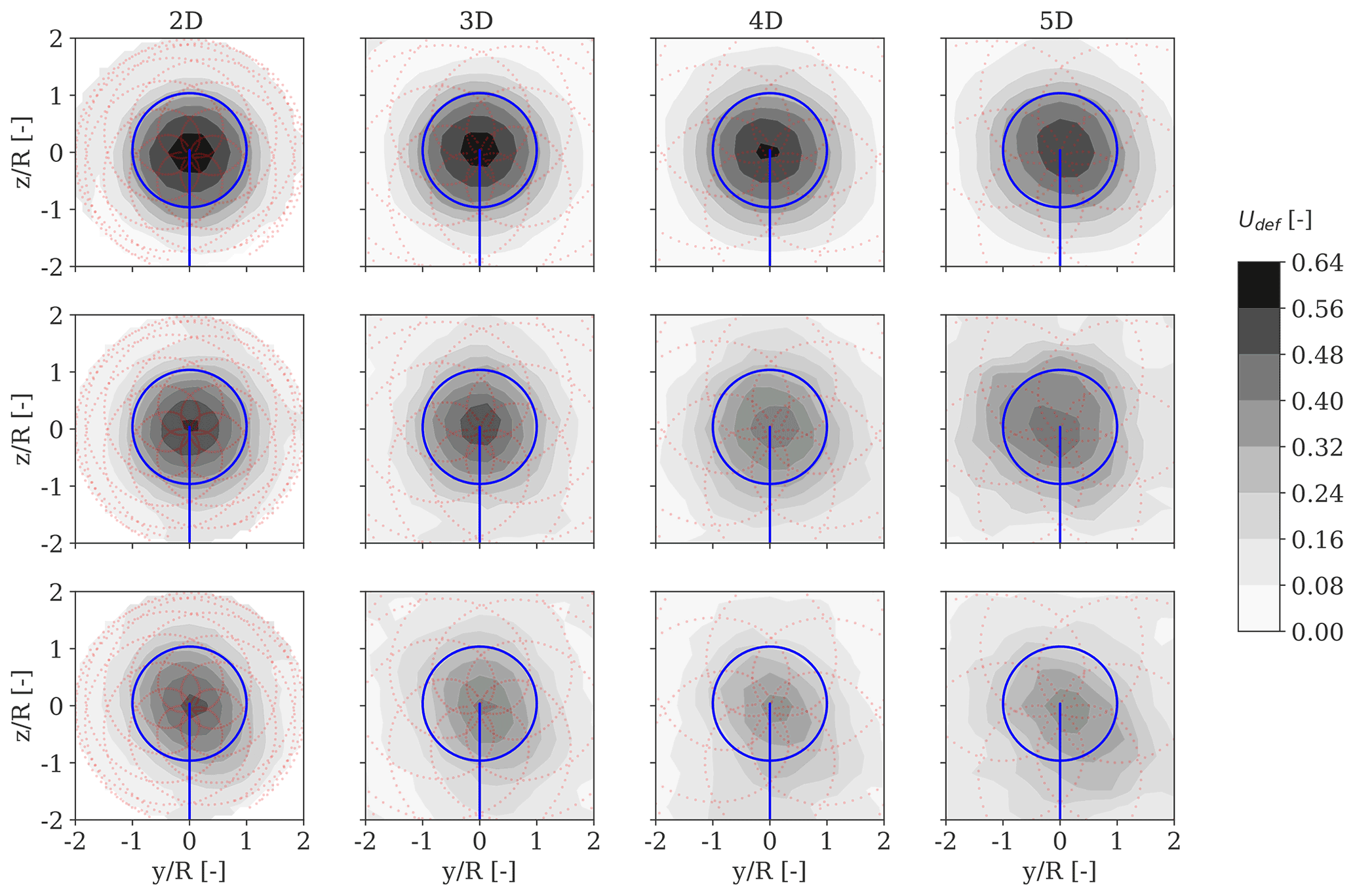
Figure 4 Ensemble-average velocity deficit profiles in the MFoR measured at 2, 3, 4, and 5 D behind the rotor for an inflow wind speed of 7 m/s under stable (upper row), near-neutral (middle-row), and unstable (lower row) conditions. The number of scans used to derive the ensemble statistics ranges between 312 and 636, depending on data availability. The SpinnerLidar scanning pattern is shown by red dots, whereas the turbine rotor area is illustrated by solid blue lines. The vertical and lateral coordinates are normalized by the rotor radius and centred at hub height.

4.2 Lidar-estimated wake turbulence

Turbulence measures derived from lidar radial velocity measurements are “filtered” because of their relatively large probe volume (Peña et al., 2017), and so they are generally lower than those obtained from sonic observations. Nevertheless, if the Doppler spectrum of the v_los is available, we can potentially circumvent the averaging effects and estimate the unfiltered variance of v_los (Peña et al., 2017; Mann et al., 2010). Mann et al. (2010) assume that the ensemble-averaged Doppler spectrum over a time period 〈S(v_los)〉 is related to the probability distribution of the v_los at the focus distance and can be computed as

$$\begin{array}{}\text{(10)}& \langle S\left(v_{\mathrm{los}}\right)\rangle =\underset{-\mathrm{\infty }}{\overset{\mathrm{\infty }}{\int }}\mathit{\phi }\left(s\right)p\left(v_{\mathrm{los}}\right|s)ds,\end{array}$$

where φ(s) is the spatial averaging function of the lidar that depends on the position along the beam s, and p(v_los|s) denotes the PDF of v_los at the location s. If we assume that the PDF of v_los is independent of s, (i.e. there is no velocity gradient along the beam), then Eq. (10) reduces to 〈S(v_los)〉=p(v_los). As a result, the v_los statistics (i.e. mean and variance) can be computed from the first and second central moments of p(v_los) as

$$\begin{array}{}\text{(11)}& \begin{array}{rl}& {\mathit{\mu }}_{v_{\mathrm{los}}}=\underset{-\mathrm{\infty }}{\overset{+\mathrm{\infty }}{\int }}{v}_{\mathrm{los}}p\left(v_{\mathrm{los}}\right)d{v}_{\mathrm{los}},\\ & {\mathit{\sigma }}_{v_{\mathrm{los}}}^{\mathrm{2}}=\underset{-\mathrm{\infty }}{\overset{+\mathrm{\infty }}{\int }}(v_{\mathrm{los}}-{\mathit{\mu }}_{v_{\mathrm{los}}}{)}^{\mathrm{2}}p(v_{\mathrm{los}})d{v}_{\mathrm{los}},\end{array}\end{array}$$

where ${\mathit{\mu }}_{v_{\mathrm{los}}}$ and ${\mathit{\sigma }}_{v_{\mathrm{los}}}^{\mathrm{2}}$ denote the mean and unfiltered variance of v_los, respectively. Nevertheless, velocity gradients along the lidar beam may appear when measuring at the wake edges, which can introduce errors in the estimated turbulence (Meyer Forsting et al., 2017). Following the procedure of Peña et al. (2019), we compute the ensemble-averaged normalized Doppler spectrum within 10 min periods by thresholding the noise-flattened spectra with a value of 1.2 and correcting them by subtracting the background spectrum. We accumulate the LOS Doppler spectra onto the regular grid of the scanned area and estimate ${\mathit{\mu }}_{v_{\mathrm{los}}}$ and ${\mathit{\sigma }}_{v_{\mathrm{los}}}^{\mathrm{2}}$ for each grid cell using Eq. (11). As discussed in Herges and Keyantuo (2019), invalid measurements occur due to the boresight and ground return as well as the return from the rotating rotor of WTGa2, if in operation. These invalid observations appear as a very high return signal in the Doppler spectrum in proximity to low wind speeds (i.e. at approximately 1 m/s) and are removed. The filtering effects due to the probe volume can be quantified by computing the ratio between filtered and unfiltered LOS variances across the rosette pattern; we find ratios in the range 0.8–0.9 at 2.5 D, which vary according to stability conditions (not shown).

Examples of 10 min ensemble-averaged Doppler spectra obtained at three fixed locations across the scanned area – a wake centre, a wake edge, and a wake-free position – are shown in Fig. 5 for an incoming wind speed of 7 m/s and ambient turbulence of 6 %. A narrow spectrum with a single-peak distribution centred at about 7 m/s for the wake-free location (green) is seen, whereas spectrum-broadening effects induced by small-scale generated turbulence are noticeable for the positions within the wake. The wake centre (red) shows a wider spectrum with a peak at a significantly lower wind speed than the incoming flow, whereas the wake edge (cyan) shows a double-peak distribution that may be partially due to the inhomogeneity of the wind field along the beam (Herges and Keyantuo, 2019) and also due to the meandering occurring within the analysed 10 min period.

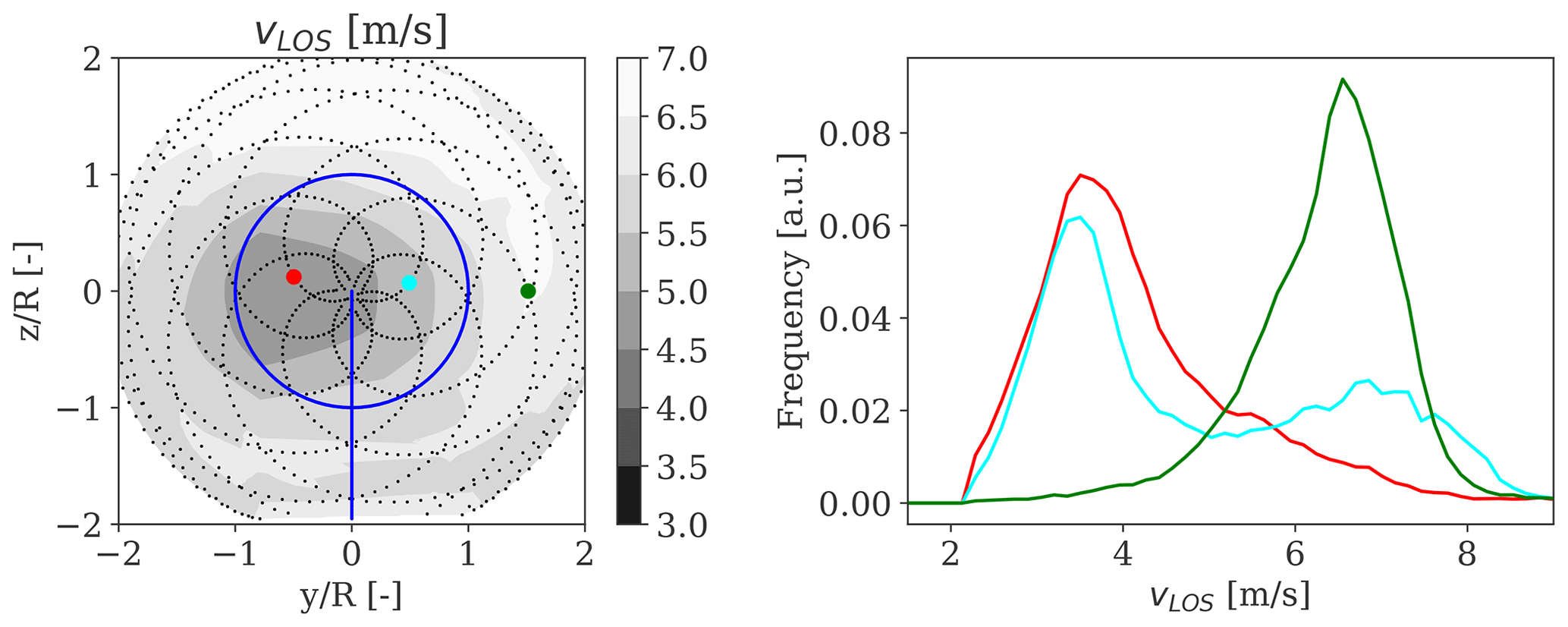
Figure 5 Examples of normalized Doppler LOS velocity spectra measured over a 10 min period at 2.5 D in the wake at three different locations – wake centre (red), wake edge (cyan), and wake-free (green) – for an incoming wind speed of 7 m/s and ambient turbulence of 6 %.

To characterize the spatial distribution of the wake turbulence within the scanned area, we derive ${\mathit{\sigma }}_{\mathrm{U}}^{\mathrm{2}}$ estimates directly by applying the variance operator to Eq. (7):

$$\begin{array}{}\text{(12)}& {\mathit{\sigma }}_{v_{\mathrm{los}}}^{\mathrm{2}}={\mathit{\sigma }}_{\mathrm{U}}^{\mathrm{2}}\cos \left(\mathit{\varphi }{)}^{\mathrm{2}}\cos \right(\mathit{\theta }-{\stackrel{\mathrm{‾}}{\mathit{\theta }}}_{\mathrm{0}}{)}^{\mathrm{2}},\end{array}$$

where ${\mathit{\sigma }}_{\mathrm{U}}^{\mathrm{2}}$ is the variance of the horizontal wind speed, and as shown, covariance terms are neglected. As the LOS is almost never aligned with the u velocity component across the rosette, except at the centre of the pattern, ${\mathit{\sigma }}_{v_{\mathrm{los}}}^{\mathrm{2}}$ can be “contaminated” by the variances and covariances of the other velocity components (Peña et al., 2017). Therefore, the relation in Eq. (12) can lead to inaccurate estimations of the longitudinal-velocity variances. Peña et al. (2019) estimated the contamination of different components on the LOS variances for the SpinnerLidar and showed that the ratio of the unfiltered LOS velocity variance to the variance of the longitudinal velocity component is generally lower than 1 across the scanned area, except at the centre, where the ratio is 1, and within an area above the centre, where it can be higher than unity. Although the adopted retrieval assumption in Eq. (12) introduces uncertainties in the turbulence measures, we can account for the expected errors in the Bayesian inference framework.

Figure 6 illustrates the spatial distribution of the unfiltered ${\mathit{\sigma }}_{\mathrm{U}}^{\mathrm{2}}$ computed in the MFoR, normalized with the u-velocity variance of the ambient wind field measured at the 32 m sonic anemometer (${\mathit{\sigma }}_{u,\mathrm{amb}}^{\mathrm{2}}$). Under stable conditions and for a downstream distance of 2.5 D, we can observe an enhancement in turbulence levels in proximity to the rotor tips, especially in the upper part of the rotor (see Fig. 6a). The observed added turbulence is caused by the breakdown of the rotor tip vortices. These features are no longer noticed as the atmosphere becomes more unstable where a more uniform and less prominent distribution of the turbulence is found (see Fig. 6b and c).

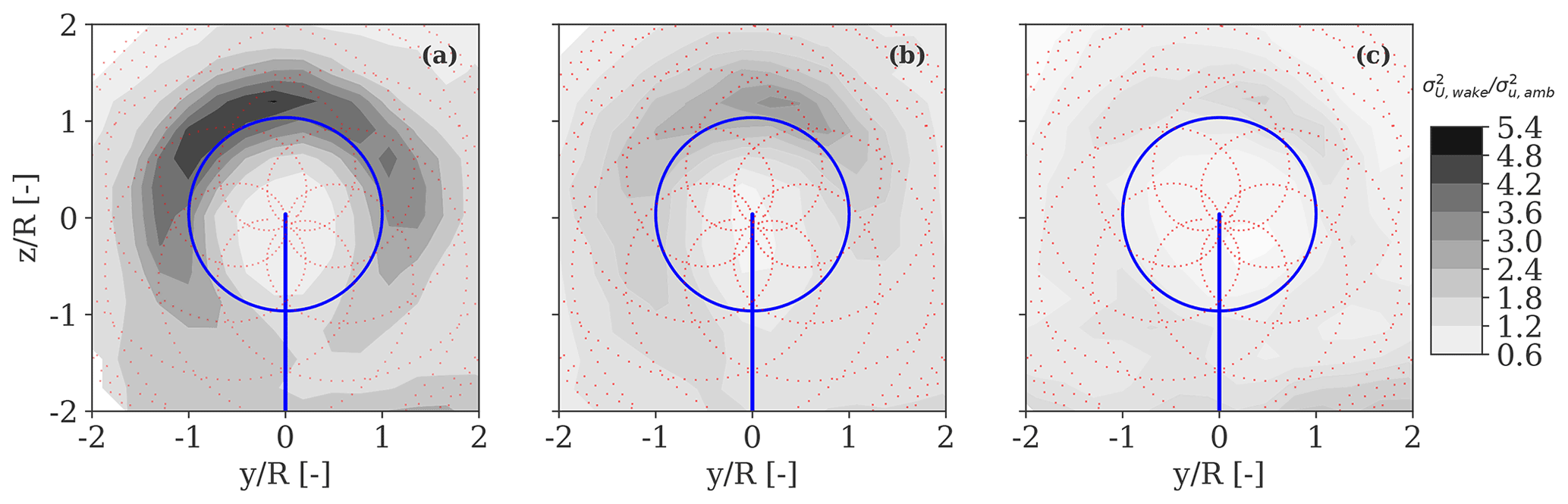
Figure 6 Two-dimensional spatial distribution of the horizontal wind velocity variance (${\mathit{\sigma }}_{\mathrm{U}}^{\mathrm{2}}$) derived in the MFoR at 2.5 D in the wake, normalized with the u-velocity variance of the ambient wind field (${\mathit{\sigma }}_{u,\mathrm{amb}}^{\mathrm{2}}$) for three 10 min periods characterized by (a) stable, (b) near-neutral, and (c) unstable conditions. Approximately 298 scans of the wake are processed for each 10 min period. The relative ambient wind speed ranges between 6.5 and 8.5 m/s.

5 Calibration of the DWM model in the MFoR

The calibration of the wake deficit and wake-added turbulence components are conducted in the MFoR using a Bayesian inference framework. We describe the Bayesian model in Sect. 5.1 and provide calibration results for the wake deficit in Sect. 5.2 and for the wake-added turbulence in Sect. 5.3. We investigate wake meandering dynamics separately in Sect. 5.4.

5.1 Bayesian inference formulation

The basis of the Bayesian inference is to estimate the probability distribution of the model parameters based on available observations. Let ${\mathit{\theta }}_{\mathrm{m}}=\mathit{\{}{k}_{\mathrm{1}},k_{\mathrm{2}},\mathrm{\dots },k_{\mathrm{m}\mathrm{1}},k_{\mathrm{m}\mathrm{2}}\mathit{\}}$ be a set of model parameters to be estimated using lidar-derived wake features (i.e. wake deficit and wake-added turbulence profiles in the MFoR) denoted by $y_{\mathrm{d}}=\mathit{\{}{y}_{\mathrm{d}\mathrm{1}},y_{\mathrm{d}\mathrm{2}},\mathrm{\dots },y_{\mathrm{dn}}\mathit{\}}$, where n is the number of available observations. We consider that the experimental data and the model predictions satisfy the prediction error equation:

$$\begin{array}{}\text{(13)}& y_{\mathrm{d}}=\widehat{g}({\mathit{\theta }}_{\mathrm{m}},X_{\mathrm{m}})+\mathit{ϵ},\end{array}$$

where $\widehat{g}({\mathit{\theta }}_{\mathrm{m}},X_{\mathrm{m}})$ denotes the DWM model predictions obtained from a particular set of model parameters (θ_m) and a set of observable variables (X_m). Here $X_{\mathrm{m}}=\mathit{\{}{\mathrm{TI}}_{\mathrm{amb}},U_{\mathrm{amb}},\mathit{\alpha },C_{\mathrm{T}},x,y,z\mathit{\}}$ includes the inflow wind conditions measured at the mast (${\mathrm{TI}}_{\mathrm{amb}},U_{\mathrm{amb}},\mathit{\alpha }$); the rotor thrust coefficient of the turbine (C_T), which is derived from the BEM model (Madsen et al., 2010); and the spatial locations of the scanning pattern ($x,y,z$). $\mathit{ϵ}={\mathit{ϵ}}_y+{\mathit{ϵ}}_{\mathrm{m}}$ denotes a random prediction error composed of two terms: the measurement error ϵ_y and the model prediction error ϵ_m. The former is described by a zero mean normal distribution with standard deviation ${\mathit{\sigma }}_{{\mathit{ϵ}}_y}$, which is determined from field observations. The latter is assumed to have zero mean, which implies unbiased model predictions, and a standard deviation ${\mathit{\sigma }}_{{\mathit{ϵ}}_{\mathrm{m}}}$ to be determined by the Bayesian estimation along with the model parameters. To facilitate statistical inference, we assume X_m as deterministic inputs (i.e. free of uncertainty) and that the model error ϵ_m is independent of the set of input variables X_m and described by a normal distribution. This implies that the model predictions are normally distributed for a given X_m, which is a reasonable choice for wake deficit profiles. The Bayesian approach for model calibration deals with updating the combined parameter set $({\mathit{\theta }}_{\mathrm{m}},{\mathit{\sigma }}_{{\mathit{ϵ}}_{\mathrm{m}}})$, given a set of observations (y_d,X_m) by applying the Bayes theorem:

$$\begin{array}{}\text{(14)}& f({\mathit{\theta }}_{\mathrm{m}},{\mathit{\sigma }}_{{\mathit{ϵ}}_{\mathrm{m}}}|y_{\mathrm{d}})={\displaystyle \frac{f\left(y_{\mathrm{d}}\right|{\mathit{\theta }}_{\mathrm{m}},{\mathit{\sigma }}_{{\mathit{ϵ}}_{\mathrm{m}}}\left)f\right({\mathit{\theta }}_{\mathrm{m}},{\mathit{\sigma }}_{{\mathit{ϵ}}_{\mathrm{m}}})}{f\left(y_{\mathrm{d}}\right)}},\end{array}$$

where $f({\mathit{\theta }}_{\mathrm{m}},{\mathit{\sigma }}_{{\mathit{ϵ}}_{\mathrm{m}}}|y_{\mathrm{d}})$ is the updated posterior distribution of the model parameters, $f({\mathit{\theta }}_{\mathrm{m}},{\mathit{\sigma }}_{{\mathit{ϵ}}_{\mathrm{m}}})$ is the prior distribution that is typically assigned based on subjective or previous information, $f\left(y_{\mathrm{d}}\right|{\mathit{\theta }}_{\mathrm{m}},{\mathit{\sigma }}_{{\mathit{ϵ}}_{\mathrm{m}}})$ denotes the likelihood of observing the data y_d from a model with corresponding θ_m parameters, and f(y_d) is the prior predictive distribution that is defined as the marginal distribution $f\left(y_{\mathrm{d}}\right)=\int f\left(y_{\mathrm{d}}\right|{\mathit{\theta }}_{\mathrm{m}},{\mathit{ϵ}}_{\mathrm{m}}\left)f\right({\mathit{\theta }}_{\mathrm{m}},{\mathit{\sigma }}_{{\mathit{ϵ}}_{\mathrm{m}}})d{\mathit{\theta }}_{\mathrm{m}}d{\mathit{ϵ}}_{\mathrm{m}}$. By using the prediction error in Eq. (13) and assuming that the error terms are jointly normal with a zero mean vector and covariance matrix ${\sum }^{{\mathit{ϵ}}_{y_{\mathrm{d}}}}=\mathrm{diag}\left({\mathit{\sigma }}_{{\mathit{ϵ}}_{y_{\mathrm{d}}}}^{\mathrm{2}}\right)$ and ${\sum }^{{\mathit{ϵ}}_{\mathrm{m}}}=\mathrm{diag}\left({\mathit{\sigma }}_{{\mathit{ϵ}}_{\mathrm{m}}}^{\mathrm{2}}\right)$, the measured quantities follow the normal distribution $y_{\mathrm{d}}\sim \mathcal{N}\left(\widehat{g}({\mathit{\theta }}_{\mathrm{m}},X_{\mathrm{m}}|y_{\mathrm{d}}),{\sum }_{\mathit{ϵ}}\right)$, where the covariance matrix takes the form ${\sum }_{\mathit{ϵ}}={\sum }^{{\mathit{ϵ}}_{y_{\mathrm{d}}}}+{\sum }^{{\mathit{ϵ}}_{\mathrm{m}}}$. As a result, the likelihood function of observing the data follows the multi-variable normal distribution defined as

$$\begin{array}{}\text{(15)}& \begin{array}{rl}& f\left(y_{\mathrm{d}}\right|{\mathit{\theta }}_{\mathrm{m}},{\mathit{ϵ}}_{\mathrm{m}})={\displaystyle \frac{{\left|{\sum }_{\mathit{ϵ}}\right|}^{-\mathrm{1}/\mathrm{2}}}{(\mathrm{2}\mathit{\pi }{)}^{n/\mathrm{2}}}}\exp \left[-{\displaystyle \frac{\mathrm{1}}{\mathrm{2}}}{\left[y_{\mathrm{d}}-\widehat{g}({\mathit{\theta }}_{\mathrm{m}},X_{\mathrm{m}}|y_{\mathrm{d}})\right]}^{\mathrm{T}}\right.\\ & \left.\sum _{\mathit{ϵ}}^{-\mathrm{1}}\left[y_{\mathrm{d}}-\widehat{g}({\mathit{\theta }}_{\mathrm{m}},X_{\mathrm{m}}|y_{\mathrm{d}})\right]\right],\end{array}\end{array}$$

where the $|.|$ denotes the determinant. The analytical and differentiable solution of the posterior distribution of the parameters in the N–S equations with the eddy viscosity term of Eq. (1) is not readily available. Therefore, we employ a numerical sampling method to approximately evaluate the posterior distribution and its first and second moments. Here, the adaptive no-U-turn Markov chain Monte Carlo (MCMC) sampler is employed to generate samples from the posterior distribution (Hoffman and Gelman, 2014; Salvatier et al., 2016).

The outcome of the calibration is a joint probability distribution of the inferred model parameters. From this joint PDF, we can estimate the posterior PDF of any wake feature simulated by the DWM model, i.e. the wake deficit and wake-added turbulence profiles in the MFoR or the fully resolved wakes in the FFoR, among others, which we denote by q:

$$\begin{array}{}\text{(16)}& f\left(q\right|y_{\mathrm{d}})=\underset{\mathrm{\Theta }}{\int }f(q\left|{\mathit{\theta }}_{\mathrm{m}}\right)f\left({\mathit{\theta }}_{\mathrm{m}}\right|y_{\mathrm{d}})d{\mathit{\theta }}_{\mathrm{m}}.\end{array}$$

The posterior distribution of the wake feature q in Eq. (16) can be solved numerically using sampling methods (e.g. Monte Carlo simulations), so its first and second moment can be estimated.

5.2 Wake deficit parameter estimation

We use lidar-derived wake deficit profiles in the MFoR collected during Strategy I and Strategy II and employ the Bayesian model to infer uncertainty in the k₁ and k₂ parameters of the eddy viscosity term in Eq. (1). These parameters were found to be the most sensitive to the resulting wake deficit predictions (Keck et al., 2012). The prediction model of Eq. (13) is constructed as follows. The experimental data (y_d) comprise two-dimensional ensemble-average lidar-estimated deficit profiles binned according to downstream distances (3, 4, and 5 D), atmospheric stability (i.e. stable, near-neutral, and unstable), and wind speed bins of 1 m/s in the range of 3–9 m/s. Note that we discard measurements in the near wake (at 2 D) for improving the quality of the fitting in the far-wake region (see Fig. 8).

The set of observable variables comprises $X_{\mathrm{m}}=\mathit{\{}{\mathrm{TI}}_{\mathrm{amb}},U_{\mathrm{amb}},\mathit{\alpha },C_{\mathrm{T}},x,y,z\mathit{\}}$, where the inflow parameters (${\mathrm{TI}}_{\mathrm{amb}},U_{\mathrm{amb}},\mathit{\alpha }$) are provided in Tables 1 and 2; the rotor thrust coefficient C_T is derived from the BEM model implemented in the aeroelastic code HAWC2 (Larsen and Hansen, 2007) and based on the aerodynamics and airfoil inputs of the SWiFT turbine (Doubrawa et al., 2020) (C_T=0.84, that is nearly constant for wind speeds below 9 m/s); and x,y, and z refer to the spatial coordinates of the deficits resolved in the MFoR. The uncertainties in measured deficit profiles are computed as ${\mathit{ϵ}}_{y_{\mathrm{d}}}\left(r\right)=\mathit{\sigma }\left(r\right)/\sqrt{n}$, where σ(r) is the standard deviation of all 10 min deficits within the analysed case at the radial position r, and n is the number of 10 min periods (also referred to as samples in Table 1).

We select uniform prior distributions on model parameters $k_{\mathrm{1},\mathrm{prior}}\sim \mathcal{U}(\mathrm{0.001},\mathrm{0.2})$ and $k_{\mathrm{2},\mathrm{prior}}\sim \mathcal{U}(\mathrm{0.001},\mathrm{0.2})$ on intervals that consider physical constraints, ensuring convergence of results and covering previous calibrations reported in the literature. Thus, we employ an MCMC algorithm to sample from the posterior PDFs of the calibration parameters using the Bayesian framework. The inferred joint and marginal posterior distributions of the model parameters (k₁ and k₂) are shown in Fig. 7, together with point values from earlier studies (Madsen et al., 2010; Keck et al., 2012; Larsen et al., 2013; IEC, 2019; Reinwardt et al., 2020). As shown, the lidar-based wake deficits are informative, and we obtain well-defined posteriors that follow a normal distribution with $k_{\mathrm{1}}\sim \mathcal{N}(\mathrm{0.081},\mathrm{0.017})$ and $k_{\mathrm{2}}\sim \mathcal{N}(\mathrm{0.015},\mathrm{0.003})$. The negative correlation between k₁ and k₂ seen in Fig. 7 indicates the interdependence of the physically induced effects as both parameters contribute to turbulence diffusion. It is found that the posterior means of the informed parameters k₁ and k₂ differ from those recommended in the IEC standard (IEC, 2019). Generally, low k₁ and k₂ values attenuate the degree of turbulence mixing in the wake, which lead to strong velocity deficits persisting at distances farther downstream. We provide the statistical properties (mean, variance, and coefficient of variation) of the inferred parameters in Table 4 and correlation measures in Table 5.

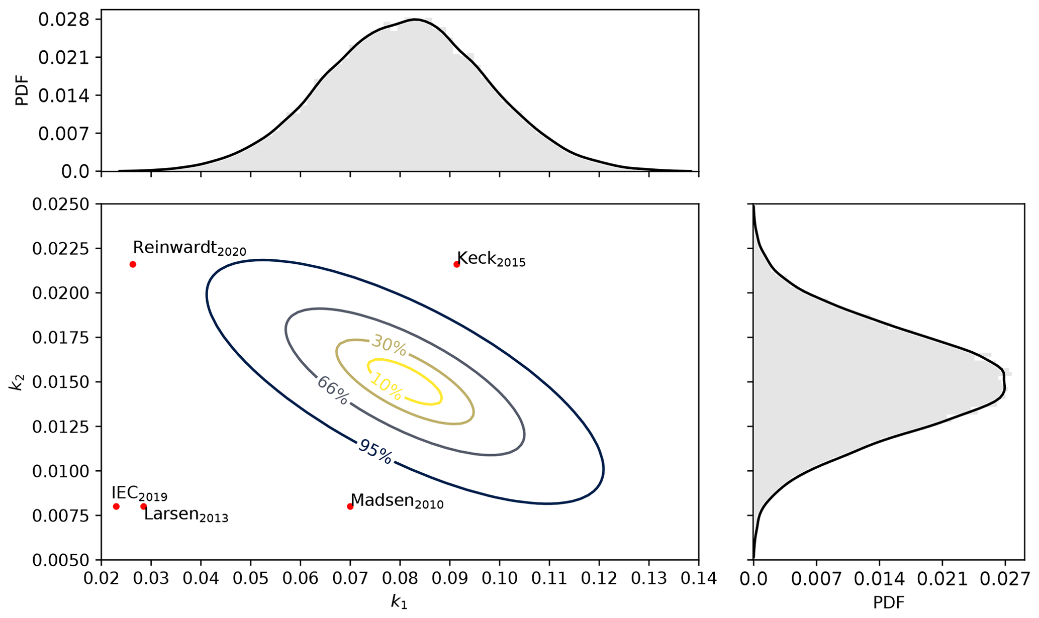
Figure 7 Joint and marginal posterior PDFs of k₁ and k₂ parameters. The uncertainty regions representing the 10 %, 30 %, 66 %, and 95 % confidence intervals are shown. The histograms obtained from 40 000 MCMC samples and the corresponding empirical PDFs are also included. The calibration parameters from early studies are shown with red markers and discussed in the text.

5.2.1 Wake deficit predictions

We propagate the uncertainties in k₁ and k₂ to predict wake deficits in the MFoR and compare them with the ensemble-average lidar-derived profiles in Fig. 8. First, we observe that the lidar-estimated deficits exhibit a faster wake recovery as the atmosphere becomes more unstable compared to stable regimes. This effect is mainly caused by the enhanced turbulence mixing occurring under unstable conditions as they are characterized by ambient turbulence levels 2–3 times higher than those of the stable cases (see Table 1). The lidar-observed maximum deficit varies between 30 % and 60 % within the first five rotor diameters, depending on the inflow turbulence conditions. Similar behaviours were reported in recent lidar measurement campaigns (Iungo and Porté-Agel, 2014; Machefaux et al., 2016; Fuertes et al., 2018; Zhan et al., 2020b).

The lidar-estimated deficits are approximately Gaussian under stable to near-neutral conditions, whereas the Gaussian shape is lost under more unstable conditions. This may result from errors in the wake tracking procedure due to the larger meandering amplitudes and also due to the presence of large-scale turbulence structures in the inflow (Conti et al., 2020a). The rotor thrust is another factor governing the variability in the wake recovery (Zhan et al., 2020b); however, its influence is secondary for the dataset analysed here due to the relatively low incoming wind speeds and relatively constant thrust coefficients (Conti et al., 2020a).

The DWM-model-predicted deficit profiles with parameters specified by their posterior distributions are in good agreement with the lidar observations for distances beyond 4 D (see Fig. 8). For these distances, the turbulence mixing effects dictated by the ambient and self-generated wake turbulence on the deficit recovery are fairly well captured by the inferred parameters. The nominal model predictions generally fit the observations, whereas an overlap between the measurements and the region of modelling uncertainty is found. The largest deviations between predicted and measured deficits are found at shorter distances (2–3 D) and are mainly due to the model inadequacy to simultaneously fit all the experimental measurements and experimental uncertainties. The assumptions adopted to describe the near-wake region also introduce uncertainty in the deficit predictions at short distances (Keck et al., 2015; Machefaux et al., 2016).

It can be observed that the uncertainties in k₁ and k₂ parameters primarily influence the depth of the wake (i.e. the maximum deficit), while the sensitivity to these parameters decreases significantly with the outer radial distance. It is also noticed that the uncertainty in the deficit predictions increases for high ambient turbulence and far downstream distances. This is because k₁ is proportional to TI_amb in Eq. (1), and the sensitivity of the model parameters increases as the wake recovers. To provide a measure of the uncertainty in wake deficit predictions, we compute the coefficient of variation COV = $\mathit{\sigma }/\mathit{\mu }$, where σ is the standard deviation, and μ is the mean value of the maximum deficit, obtained by propagating the PDFs of k₁ and k₂, as in Eq. (16). We find COV=3 % under stable conditions (T_amb=0.07), which increases to 6 % under unstable conditions (T_amb=0.14), for an incoming wind speed of 7 m/s. This result confirms that the uncertainty in wake deficit predictions increases for higher turbulence, but it also shows that uncertainties in k₁ and k₂ parameters do not lead to uncertainty of the same magnitude in deficit predictions resolved in the MFoR (for reference, ${\mathrm{COV}}_{k_{\mathrm{1}}}=\mathrm{21}$ % and ${\mathrm{COV}}_{k_{\mathrm{2}}}=\mathrm{19}$ %, as reported in Table 4).

We provide comparisons between measured and predicted wake deficit profiles using the calibration from this work as well as those reported in early studies in Fig. 9. For this particular analysis, we analyse predictions at 5 D behind the rotor for an inflow wind speed of 7 m/s under stable, near-neutral, and unstable regimes. The main discrepancy among the models is the relative sensitivity of the wake recovery to the ambient turbulence. This is primarily governed by k₁; however, in the eddy viscosity model of Larsen et al. (2013), IEC (2019), and Reinwardt et al. (2020), it also depends on a nonlinear coupling function F_amb(TI_amb) that attenuates the wake recovery for turbulence above ≈12 % (see Fig. 6 in Larsen et al., 2013). This function was introduced to fit the power productions at the Egmond aan Zee offshore wind farm, and it is not based on observations of the wake field (Larsen et al., 2013). The wake recovery predicted with the models of Larsen et al. (2013) and IEC (2019) is practically insensitive to ambient turbulence rising from 7 % to 16 % at downstream distances up to 5 D. Similar outcomes are reported in Fig. 13 in Reinwardt et al. (2020), who showed that the model of Larsen et al. (2013) provided conservative deficits for ambient turbulence up to 16 %.

By considering k₁ and k₂ as universal constants (Keck et al., 2012), the quality of the dataset utilized for the model calibration is essential to ensure reliable parameter estimation. As previous calibrations were carried out on larger rotors than those of the SWiFT turbines and utilized either power production data (Larsen et al., 2013; IEC, 2019) or limited CFD simulations (Madsen et al., 2010; Keck et al., 2015) and one-dimensional scans of the wake by a nacelle lidar (Reinwardt et al., 2020), these aspects may explain the observed deviations in Fig. 9.

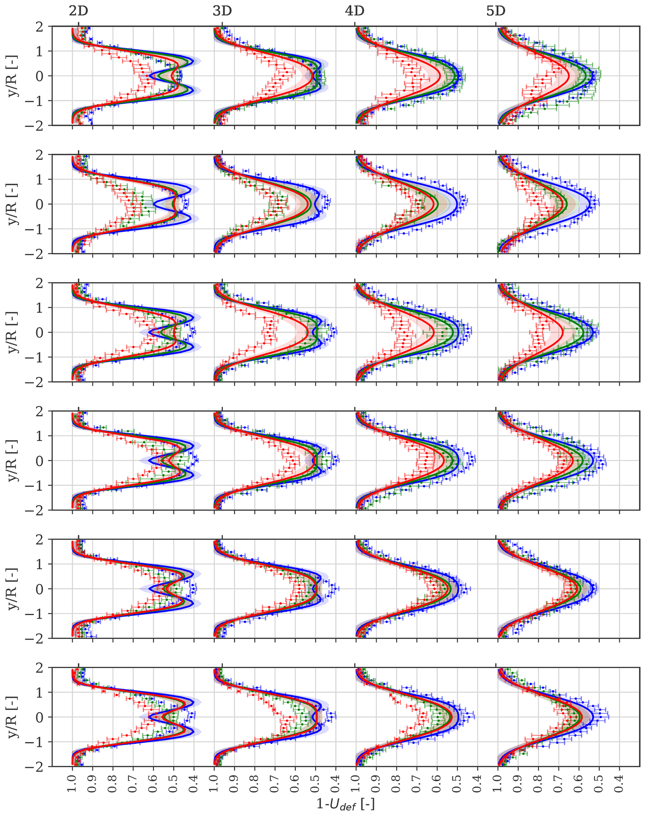
Figure 8 Comparison between measured and predicted ensemble-average spanwise velocity deficit profiles resolved in the MFoR at hub height and obtained at 2, 3, 4, and 5 D behind the rotor (from left to right) and for inflow wind speeds ranging from 3 to 8 m/s with a 1 m/s bin (from top to bottom panel). The SpinnerLidar-measured (markers) and DWM-model-predicted (solid lines) deficits are shown for each stability class (stable in blue, near-neutral in green, and unstable in red). The error bars represent the measurement uncertainty, while the shaded areas represent the uncertainty in the model predictions; both sources of uncertainty refer to the 95 % confidence interval (see Table 1 for details on the inflow wind conditions).

Figure 9 Ensemble-average spanwise velocity deficit profiles computed in the MFoR at hub height obtained at 5 D behind the rotor for an incoming wind speed of 7 m/s under stable (blue), near-neutral (green), and unstable (red) atmospheric conditions. The measured turbulence intensities are 7 %, 12 %, and 16 %, respectively. The SpinnerLidar-measured profiles are shown by markers and their relative 95 % confidence interval by the error bars. The DWM-model-predicted deficits are shown by solid lines; each panel refers to model predictions using calibration parameters from a number of studies (see text for more details). The “SpinnerLidar” panel refers to the model proposed in the current study, while the shaded areas indicate its 95 % confidence interval.

5.3 Improved wake-added turbulence formulation

The wake-added turbulence model (Eq. 3) assumes that turbulent structures (i.e. tip and root vortices) are unaffected by atmospheric turbulence. The rotor-induced vortices are rapidly disrupted under high-turbulence conditions, causing the breakdown within the first 2 D (Madsen et al., 2005). However, vortices can persist and extend at farther distances under low to moderate turbulence combined with stable stratification conditions (Ivanell et al., 2009; Subramanian et al., 2018; Conti et al., 2020a). Thus, the wake-added turbulence profiles can exhibit a more pronounced double-peak feature in the proximity of the rotor tips or a more uniform distribution depending on the atmospheric turbulence conditions (this effect is also seen in Fig. 6). Equation (3) also assumes radially symmetric wake-added turbulence profiles. However, the inflow vertical wind shear re-distributes the wake turbulence. Enhanced turbulence levels are actually observed in the proximity of the upper tip of the rotor blade (Vermeer et al., 2003; Chamorro and Porte-Agel, 2009; Conti et al., 2020a). Figure 6a shows this effect.

Due to these two assumptions, we propose an improved semi-empirical formulation of the wake-added turbulence scaling factor $k_{\mathrm{mt}}^{*}$, which produces wake profiles in better agreement with the lidar observations. This is achieved by relating both the depth and the velocity gradient terms to the ambient turbulence and by including the effect of the inflow vertical wind shear on the vertical-velocity deficit gradient as

$$\begin{array}{}\text{(17)}& \begin{array}{rl}{k}_{\mathrm{mt}}^{*}(y,z)& =\mid \mathrm{1}-U_{\mathrm{def}}(y,z)\mid (k_{\mathrm{m}\mathrm{1}}^{*}{\mathrm{TI}}_{\mathrm{amb}}+k_{q\mathrm{1}}^{*})\\ & +\left|{\displaystyle \frac{\partial U_{\mathrm{def}}^{*}(y,z)}{\partial y\partial z}}\right|(k_{\mathrm{m}\mathrm{2}}^{*}{\mathrm{TI}}_{\mathrm{amb}}+k_{q\mathrm{2}}^{*}),\end{array}\end{array}$$

where $U_{\mathrm{def}}^{*}(y,z)=\left(U\right(z\left)U_{\mathrm{def}}\right(y,z\left)\right)/\max$ (U(z)U_def(y,z)), and $k_{\mathrm{m}\mathrm{1}}^{*},k_{q\mathrm{1}}^{*},k_{\mathrm{m}\mathrm{2}}^{*}$, and $k_{q\mathrm{2}}^{*}$ are parameters to be determined using Bayesian inference. Figure 10 illustrates the two-dimensional profiles of the depth and velocity deficit gradient terms of Eqs. (3) and (17). As illustrated, by including the term $U_{\mathrm{def}}^{*}(y,z)$, we obtain a turbulence field that mimics qualitatively well the observed enhanced turbulence within the upper wake region.

Figure 10 DWM-model-predicted flow characteristics. (a) Velocity deficit, (b) velocity deficit term with combined vertical shear profile $U_{\mathrm{def}}(y,z{)}^{*}$, (c) gradient of the velocity deficit, (d) gradient of the profile resulting from the combined velocity deficit and the vertical shear. The flow characteristics are computed for U_amb=6 m/s, TI_amb=7 %, and α=0.25 at a downstream distance of 2.5 D.

5.3.1 Estimation of wake-added turbulence parameters

The calibration parameters in Eq. (17) are inferred based on the lidar-estimated wake-added turbulence profiles in the MFoR collected during Strategy II. For this particular dataset, the SpinnerLidar scans at a fixed distance of 2.5 D, ensuring about 298 scans for every 10 min period. The inflow characteristics are reported in Table 2. As the Doppler LOS velocity spectrum is available, we derive unfiltered LOS variances as described in Sect. 4.2 and subsequently the turbulence intensity as the ratio of the standard deviation to the mean of the horizontal wind speed. From Eq. (2), we can isolate TI_add (wake-added turbulence term) by firstly resolving the wake recordings in the MFoR, which eliminates the contribution of TI_m, and then by subtracting TI_amb, which is derived from the 32 m sonic observations in front of the rotor.

As a first step, we fit the “original” analytical formulation of k_mt from Eq. (3) to each individual lidar-estimated wake-added turbulence profile to estimate the values of k_m1 and k_m2 using a simple least-squares optimization algorithm. Figure 11a and d show the relation between the estimated optimal parameters (in markers) and the ambient turbulence. It is shown that k_m1 increases, and k_m2 decreases almost linearly for increasing turbulence intensity. This indicates the strong effect of the deficit gradient term (proportional to k_m2 in Eq. 3) under low-turbulence conditions, which both amplifies the double-peak feature of the wake turbulence profile at the rotor tips and mimics the wake vortices. As the ambient turbulence increases, k_m1 and lower k_m2 become larger, which indicates a more uniform distribution of the wake turbulence. These effects are observed in Fig. 11b and c (see markers), which show the spanwise distribution of the lidar-derived wake-added turbulence for two 10 min periods with relatively low and high values of ambient turbulence intensity, 7 % and 12 %, respectively. We also compare the measured and predicted vertical distribution of TI_add in Fig. 11e and f, which shows that slightly improved predictions can be obtained using Eq. (17), i.e. considering the effects of the atmospheric shear on wake turbulence.

To infer the posterior PDFs of $k_{\mathrm{m}\mathrm{1}}^{*},k_{q\mathrm{1}}^{*},k_{\mathrm{m}\mathrm{2}}^{*}$, and $k_{q\mathrm{2}}^{*}$, we assign prior distributions based on the linear dependencies observed in Fig.11a and d, namely $k_{\mathrm{m}\mathrm{1},\mathrm{prior}}\sim \mathcal{U}(\mathrm{0},\mathrm{6})$, $k_{q\mathrm{1},\mathrm{prior}}\sim \mathcal{U}(\mathrm{0},\mathrm{0.1})$, $k_{\mathrm{m}\mathrm{2},\mathrm{prior}}\sim \mathcal{U}(-\mathrm{50},\mathrm{10})$, and $k_{q\mathrm{2},\mathrm{prior}}\sim \mathcal{U}(\mathrm{0},\mathrm{5})$ as well as $k_{\mathrm{1}}\sim \mathcal{N}(\mathrm{0.081},\mathrm{0.017})$ and $k_{\mathrm{2}}\sim \mathcal{N}(\mathrm{0.015},\mathrm{0.003})$ previously estimated in Sect. 5.2. The uncertainties in lidar-derived wake-added turbulence profiles account for errors introduced by the flow modelling assumptions of Eq. (12), which neglects cross-contamination effects on the LOS variance. We define these errors as zero-mean normally distributed with standard deviation ${\mathit{\sigma }}_{{\mathit{ϵ}}_{y_{\mathrm{d}}}}=\mathrm{0.1}\cdot T_{\mathrm{add}}(y,z)$, which leads to a coefficient of variation of 10 % (Peña et al., 2019).

The resulting posterior PDFs of the parameters follow a normal distribution (not shown) with statistical properties tabulated in Table 4. We provide the mean values of the inferred $k_{\mathrm{m}\mathrm{1}}^{*},k_{q\mathrm{1}}^{*},k_{\mathrm{m}\mathrm{2}}^{*}$, and $k_{q\mathrm{2}}^{*}$ values in the form of a linear regression model that relates the depth and deficit gradient terms of Eq. (17) to the ambient turbulence in Fig. 11a and d. The shaded area represents the 95 % confidence interval, which is obtained by propagating the PDFs of the turbulence-related and wake deficit parameters. As shown, the predictions are characterized by a relatively high degree of uncertainty. This is because, for example, there are few available observations to characterize turbulence; the measurement uncertainties are relatively high; and the modelling simplifications, such as the semi-empirical $k_{\mathrm{mt}}^{*}$, introduce further uncertainties. We provide the correlations among all the inferred parameters obtained from the joint PDF in Table 5. As expected, the wake deficit parameters k₁ and k₂ are negatively correlated to $k_{\mathrm{m}\mathrm{1}}^{*}$ and $k_{q\mathrm{1}}^{*}$ as $k_{\mathrm{m}\mathrm{1}}^{*}$ and $k_{q\mathrm{1}}^{*}$ are proportional to the wake deficit term in Eq. (17), which is the main driver to the intensity of the wake-added turbulence.

Figure 11 Wake-added turbulence predictions. Panels (a) and (d) show the relation of both k_m1 and k_m2 in Eq. (3) to the ambient turbulence. The linear regression model that is determined using Bayesian inference is shown by solid lines, whereas the shaded areas indicate the 95 % confidence interval obtained by propagating the posterior PDFs of the parameters. The comparison between measured (markers) and predicted (lines) lateral wake-added turbulence profiles resolved in the MFoR at hub height and obtained at 2.5 D behind the rotor is shown in (b) and (c) for TI_amb = 7 % and 12 %, respectively, whereas the relative vertical profiles are shown in (e) and (f). The error bars indicate the measurement uncertainty, whereas the shaded areas indicate that of the model predictions relative to the 95 % confidence interval. The predictions from Eq. (3) are computed using the mean values of k_m1=0.11 and k_m2=0.54, which are obtained from all the observations in (a) and (d).

5.4 Wake meandering

Here, we investigate the relationship between the inflow turbulence fluctuations and the lidar-tracked wake positions to characterize the large-scale eddies responsible for the meandering. The analysis is carried out by comparing the spectra of the lidar-tracked meandering time series, which are derived by means of the tracking algorithm in Eq. (9), with that simulated from the meandering model in Eq. (4), where v_c and w_c are obtained from the sonic observations at 32 m. Yaw misalignment from SCADA is also included. We conduct the analysis using the dataset collected at 2.5 D behind the rotor during Strategy II and classify all the available 10 min periods according to stability to derive ensemble-average spectra from multiple observations with similar inflow conditions. Note that the measured inflow wind speeds are below rated, and turbulence levels from all 10 min periods within each stability class are similar to those reported in Table 2.

Results of the spectral analysis for both lateral and vertical meandering are shown in Fig. 12. Here, the ensemble-average spectra from the SpinnerLidar observations are compared to those from the meandering model without low-pass filtering the incoming turbulence fluctuations (denoted as DWM^wf). The spectra are normalized with their relative variances and plotted as a function of the commonly used Strouhal number $St=fD/U_{\mathrm{\infty }}$, where f denotes frequency, and U_∞ is the aggregated wind speed from the ensemble-average statistics. As shown, the slope of the lidar-based spectra (red lines) matches that of DWM^wf (blue lines) up to St = 0.3–0.5, which corresponds to three and two rotor diameters, respectively. For St> 0.5, the energy content of the lidar-estimated spectra remarkably decreases compared to that of DWM^wf. These observations indicate that large-scale turbulent structures (>2 D) are dominant in the wake meandering (Trujillo et al., 2011; Heisel et al., 2018). When compared to the stable case, the spectra under unstable conditions show a higher energy content at large turbulence scales or equivalently low Strouhal number.

Figure 12 shows that a stochastic description of the large-scale eddy size might be appropriate. Thus, we describe the large-scale eddies responsible for the wake meandering by introducing the stochastic variable D_m, which is normally distributed with a mean equal to 2.5 D (it corresponds to the wake diameter at 5 D behind the rotor) and a standard deviation of 0.3 D based on the observations in Fig. 12. The resulting 95 % confidence intervals are shown as shaded areas in Fig. 12. The uncertainty in D_m is found negligible when computing wake meandering time series; this is shown in Appendix A.

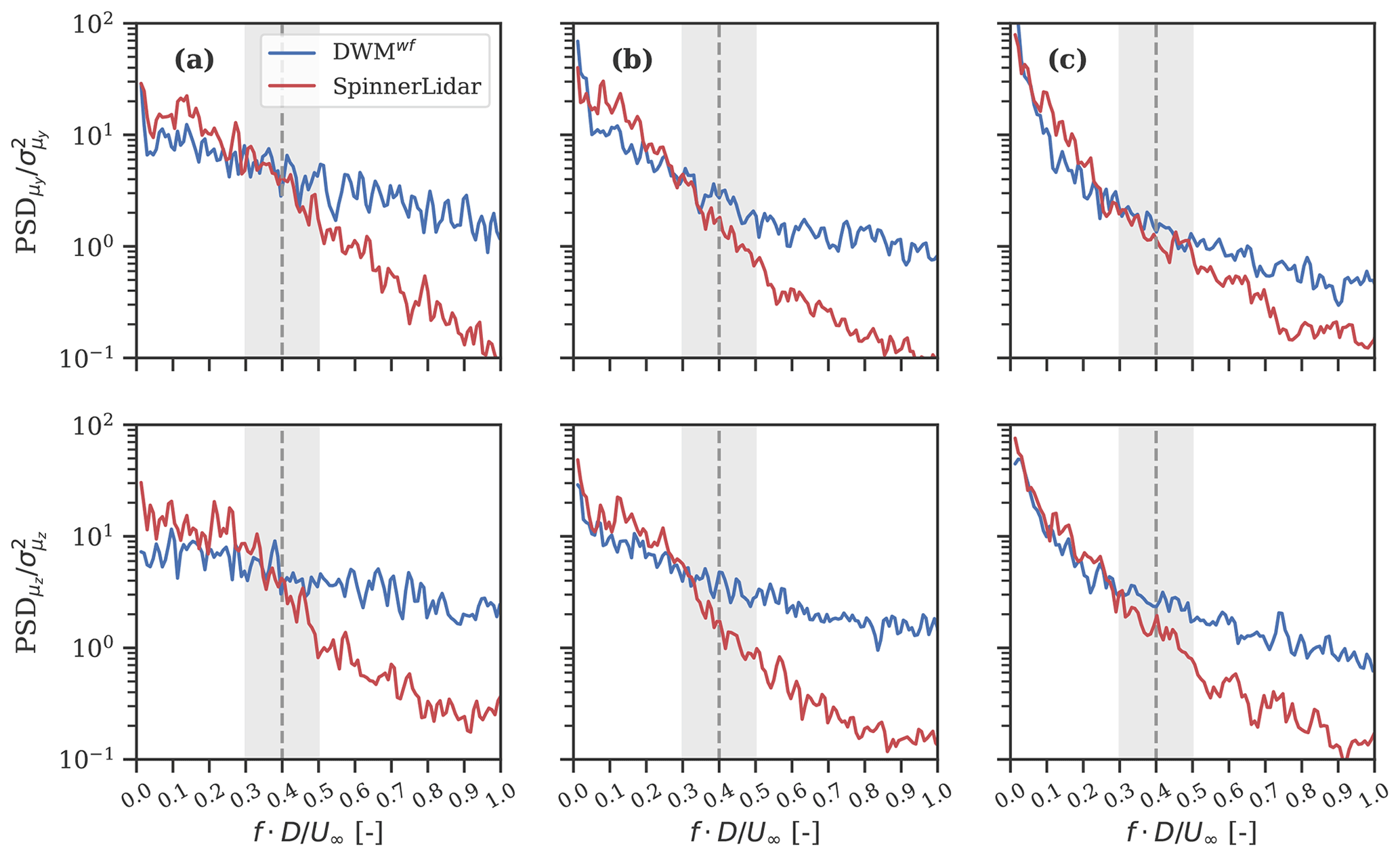
Figure 12 Normalized ensemble-average power spectral density (PSD) of the lateral and vertical wake meandering tracked by the SpinnerLidar (red) and that derived using the meandering model (DWM^wf; shown in blue) under stable (column a), near-neutral (column b), and unstable conditions (column c). The ensemble-average PSDs are computed for data collected at 2.5 D behind the rotor and are normalized with their relative variances. The 95 % confidence interval in the large-scale-eddy definition is shown by the grey area (see text for more details).

6 Validation of the DWM model in the FFoR

The validation of the DWM model is performed by resolving wake fields in the FFoR; thus the simulated wakes include the combined effects of the velocity deficit, added turbulence, and wake meandering dynamics in both lateral and vertical directions. This analysis is carried out using data from Strategy III, i.e. at a fixed distance of 5 D behind the rotor, ensuring a sufficient number of scans to derive unfiltered turbulence estimates as well as wake meandering time series within a 10 min period. The analysed dataset is primarily characterized by stable conditions, as seen in Table 3, i.e. low turbulence intensities (6 %–8 %) and strong vertical shears (α = 0.18–0.38).

6.1 Correction for rotor induction effects

The SpinnerLidar measurements collected during Strategy III were taken in the induction zone of the WTGa2 (Herges et al., 2018). For induction correction, we employ the two-dimensional induction model of Troldborg and Meyer Forsting (2017), which accounts for both longitudinal and radial variation in the induced wind velocity:

$$\begin{array}{}\text{(18)}& \begin{array}{rl}& C_{\mathrm{ind}}=\\ & \left[\mathrm{1}-a_{\mathrm{0}}\left(\mathrm{1}-{\displaystyle \frac{{\mathit{\xi }}_x}{\sqrt{\mathrm{1}+{\mathit{\xi }}_x^{\mathrm{2}}}}}\right)\cdot {\left({\displaystyle \frac{\mathrm{2}}{\exp (+{\mathit{\beta }}_a{\mathit{ϵ}}_a)+\exp (-{\mathit{\beta }}_a{\mathit{ϵ}}_a)}}\right)}^{\mathrm{2}}\right],\end{array}\end{array}$$

where a₀ is the induction factor at the rotor centre area, $a_{\mathrm{0}}=\mathrm{0.5}(\mathrm{1}-\sqrt{\mathrm{1}-{\mathit{\gamma }}_a{C}_{\mathrm{T}}})$; γ_a=1.1, ${\mathit{\xi }}_x=x/R$ is the distance in front of the rotor normalized by the rotor radius; ${\mathit{\rho }}_a=\sqrt{y^{\mathrm{2}}+z^{\mathrm{2}}}/R$ denotes the radial distance from the rotor centre axis; and ${\mathit{ϵ}}_a={\mathit{\rho }}_a/\sqrt{{\mathit{\lambda }}_a({\mathit{\eta }}_a+{\mathit{\xi }}_x^{\mathrm{2}})}$, ${\mathit{\beta }}_a=\sqrt{\mathrm{2}}$, λ_a=0.587, and η_a=1.32 (Troldborg and Meyer Forsting, 2017; Dimitrov, 2019). Note that only lidar measurements taken across the rotor area of WTGa2 are corrected by the induction factor in Eq. (18). The estimated induction factors indicate that the wind speed can be reduced at hub height by up to 12 % upstream of the WTGa2 and below rated power (see also Fig. 14).

6.2 Uncertainty propagation of simulated wake fields

We derive the two-dimensional spatial distribution of the mean wind speed in the wake region (U_FFoR) by the convolution between the wake deficit in the MFoR (U_def, MFoR) and the PDF of the meandering path (f_m) (Keck et al., 2015):

$$\begin{array}{}\text{(19)}& \begin{array}{rl}& U_{\mathrm{FFoR}}(y,z,k_{\mathrm{1}},k_{\mathrm{2}},D_{\mathrm{m}},y_{\mathrm{m},\mathit{ϵ}},z_{\mathrm{m},\mathit{ϵ}})=\\ & U_{\mathrm{amb}}{\left({\displaystyle \frac{z}{z_{\mathrm{hub}}}}\right)}^{\mathit{\alpha }}\int \int U_{\mathrm{def},\mathrm{MFoR}}(y-y_{\mathrm{m}}+y_{\mathrm{m},\mathit{ϵ}},z-z_{\mathrm{m}}\\ & +z_{\mathrm{m},\mathit{ϵ}},k_{\mathrm{1}},k_{\mathrm{2}})\cdot f_{\mathrm{m}}(y_{\mathrm{m}},z_{\mathrm{m}},D_{\mathrm{m}},y_{\mathrm{m},\mathit{ϵ}},z_{\mathrm{m},\mathit{ϵ}})d{y}_{\mathrm{m}}d{z}_{\mathrm{m}},\end{array}\end{array}$$

where y_m and z_m denote the spatial coordinates of the wake meandering time series, and y_m, ϵ and z_m, ϵ are measures of their relative uncertainties. We introduce these errors to account for incorrect wake tracking positions that can arise due to the adopted wake tracking algorithm; y_m, ϵ and z_m, ϵ are assumed to be uncorrelated and to follow a normal distribution with zero mean and standard deviation such that the 95 % percentile corresponds to approximately 4 m, which is twice the resolution adopted to interpolate SpinnerLidar measurements onto the regular grid (see Sect. 4). Note that the atmospheric shear profile U_amb(z) is superposed after the wake deficit calculation (Madsen et al., 2010). Similarly, the two-dimensional spatial distribution of the u-velocity variance (${\mathit{\sigma }}_{u_{\mathrm{FFoR}}}^{\mathrm{2}}$) can be computed as

$$\begin{array}{}\text{(20)}& \begin{array}{rl}& {\mathit{\sigma }}_{u_{\mathrm{FFoR}}}^{\mathrm{2}}(y,z,k_{\mathrm{1}},k_{\mathrm{2}},k_{\mathrm{m}\mathrm{1}}^{*},k_{q\mathrm{1}}^{*},k_{\mathrm{m}\mathrm{2}}^{*},k_{q\mathrm{2}}^{*},D_{\mathrm{m}},y_{\mathrm{m},\mathit{ϵ}},z_{\mathrm{m},\mathit{ϵ}})=\\ & {\mathit{\sigma }}_{u_{\mathrm{amb}}}^{\mathrm{2}}+\int \int \left(\right(U_{\mathrm{MFoR}}(y-y_{\mathrm{m}}+y_{\mathrm{m},\mathit{ϵ}},z-z_{\mathrm{m}}+z_{\mathrm{m},\mathit{ϵ}},k_{\mathrm{1}},k_{\mathrm{2}})\\ & -U_{\mathrm{FFoR}}(y,z,k_{\mathrm{1}},k_{\mathrm{2}},D_{\mathrm{m}},y_{\mathrm{m},\mathit{ϵ}},z_{\mathrm{m},\mathit{ϵ}}){)}^{\mathrm{2}}+(k_{\mathrm{mt},\mathrm{MFoR}}^{*}\left(y\right.\\ & -y_{\mathrm{m}}+y_{\mathrm{m},\mathit{ϵ}},z-z_{\mathrm{m}}+z_{\mathrm{m},\mathit{ϵ}},k_{\mathrm{1}},k_{\mathrm{2}},k_{\mathrm{m}\mathrm{1}}^{*},k_{q\mathrm{1}}^{*},k_{\mathrm{m}\mathrm{2}}^{*},k_{q\mathrm{2}}^{*})\\ & {\left.\cdot U_{\mathrm{MFoR}}(y-y_{\mathrm{m}}+y_{\mathrm{m},\mathit{ϵ}},z-z_{\mathrm{m}}+z_{\mathrm{m},\mathit{ϵ}},k_{\mathrm{1}},k_{\mathrm{2}})\right)}^{\mathrm{2}})\\ & \cdot f_{\mathrm{m}}(y_{\mathrm{m}},z_{\mathrm{m}},D_{\mathrm{m}},y_{\mathrm{m},\mathit{ϵ}},z_{\mathrm{m},\mathit{ϵ}})d{y}_{\mathrm{m}}d{z}_{\mathrm{m}},\end{array}\end{array}$$

where $U_{\mathrm{MFoR}}=U_{\mathrm{amb}}\left(z\right)U_{\mathrm{def},\mathrm{MFoR}}$, U_FFoR is derived from Eq. (19), and ${\mathit{\sigma }}_{u_{\mathrm{amb}}}^{\mathrm{2}}$ is the variance of the ambient u velocity component. Alternatively, U_FFoR and ${\mathit{\sigma }}_{u_{\mathrm{FFoR}}}^{\mathrm{2}}$ can be equivalently derived by superposing the wake deficit and the wake-added turbulence factor $k_{\mathrm{mt}}^{*}$ on stochastic turbulence fields with constrained meandering path and subsequently by computing the first- and second-order statistics of the synthetic wind fields. However, the analytical forms in Eqs. (19) and (20) can be easily used to propagate the posterior PDFs of the calibration parameters to predict profiles of U_FFoR and ${\mathit{\sigma }}_{u_{\mathrm{FFoR}}}$ with relative uncertainties. The inflow parameters (U_amb, α, and ${\mathit{\sigma }}_{u_{\mathrm{amb}}}^{\mathrm{2}}$) in Eqs. (19) and (20) are required inputs for the DWM model and are estimated from mast measurements.

Table 4 Mean (μ), standard deviation (σ), and coefficient of variation (COV$=\mathit{\sigma }/\mathit{\mu }$) estimated from the posterior PDFs of model parameters. The values of k₁, k₂, ${\mathit{\sigma }}_{{\mathit{ϵ}}_{\mathrm{def}}}$, k_m1, k_q1, k_m2, k_q2, and ${\mathit{\sigma }}_{{\mathit{ϵ}}_{\mathrm{add}}}$ are determined using Bayesian inference. D_m denotes the spatial size of the large-scale eddies governing wake meandering dynamics, and y_m, ϵ and z_m, ϵ denote the wake tracking position errors expressed in metres.

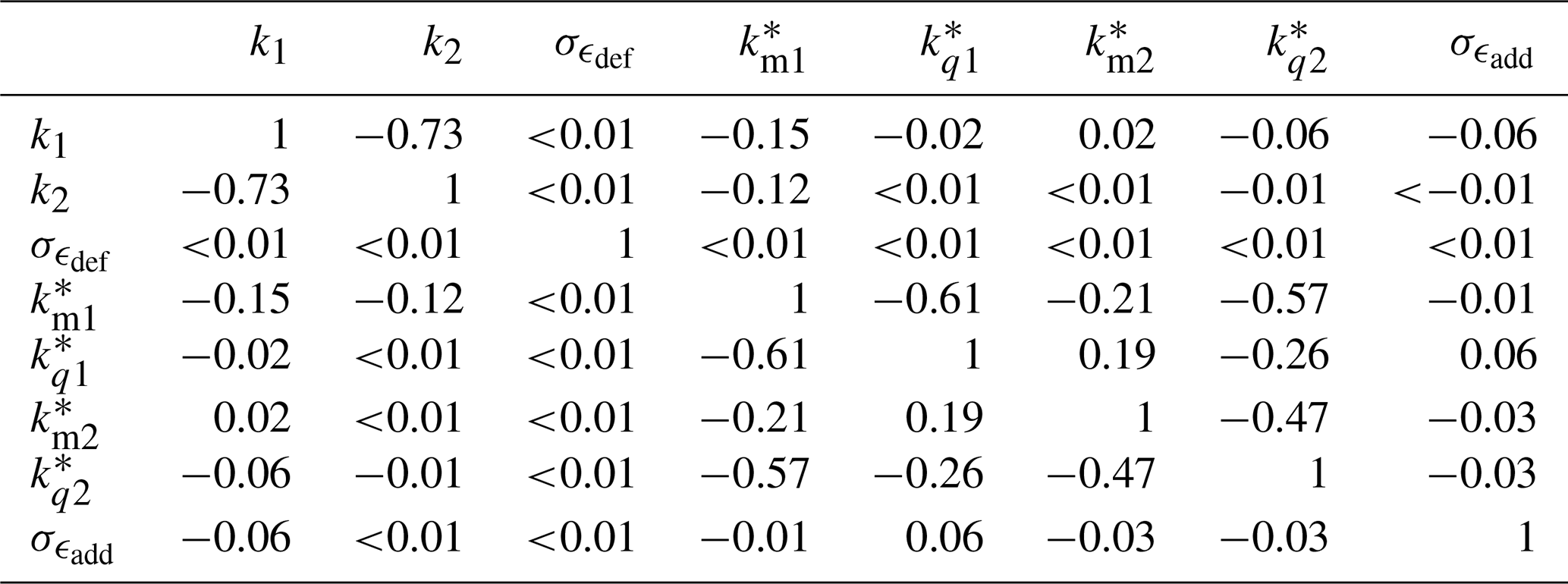
Table 5 Correlation coefficients between model parameters estimated using Bayesian inference.

We compute U_FFoR and ${\mathit{\sigma }}_{u_{\mathrm{FFoR}}}$ from Eqs. (19) and (20) by constraining the meandering path (f_m) using either the lidar-tracked meandering time series, which we denote as DWM^*, or by using the meandering model in Eq. (4) with low-pass-filtered v_c- and w_c-velocity fluctuations obtained from the 32 m sonic anemometer and the yaw misalignment of WTGa1 obtained from SCADA, which we denote as DWM${}^{**}$. In the latter model, the low-pass-filtered frequency is defined as a function of the stochastic variable associated with the size of the large-scale eddies (D_m), as discussed in Sect. 5.4. Figure 13 shows the comparison between observed and predicted (with both DWM^* and DWM${}^{**}$ models) profiles of the mean wind speed and its standard deviation obtained from two different 10 min periods.

A good agreement between measurements and predictions is found. The vertical profile of the mean wind speed exhibits a single-peak shape resulting from the combined effects of the inflow vertical shear (modelled by a power law) and the wake-induced Gaussian-like deficit shape. The wake turbulence in the lateral direction exhibits a double-peak shape with larger values near the locations associated with strong velocity gradients that are further enhanced by the wake meandering. Enhanced turbulence levels in proximity of the upper wake region are observed from lidar measurements. The deviations between DWM^* and ${\mathrm{DWM}}^{**}$ model predictions are more pronounced for the simulated turbulence than for the wind speed fields and are exclusively due to differences in the meandering representations.

The wake simulation uncertainties shown in Fig. 13 are determined by propagating uncertainties in model parameters (Table 4) and by accounting for relative correlations (Table 5) using Monte Carlo simulations. The uncertainties in lidar-measured wind speeds account for volume averaging effects and for errors introduced by the retrieval assumptions (e.g. wsin (ϕ)=0 m/s) (Debnath et al., 2019). The uncertainties in lidar-derived turbulence (here defined as the standard deviation of the wind speed) account for errors introduced by neglecting cross-contamination effects in Eq. (12) (Peña et al., 2019).

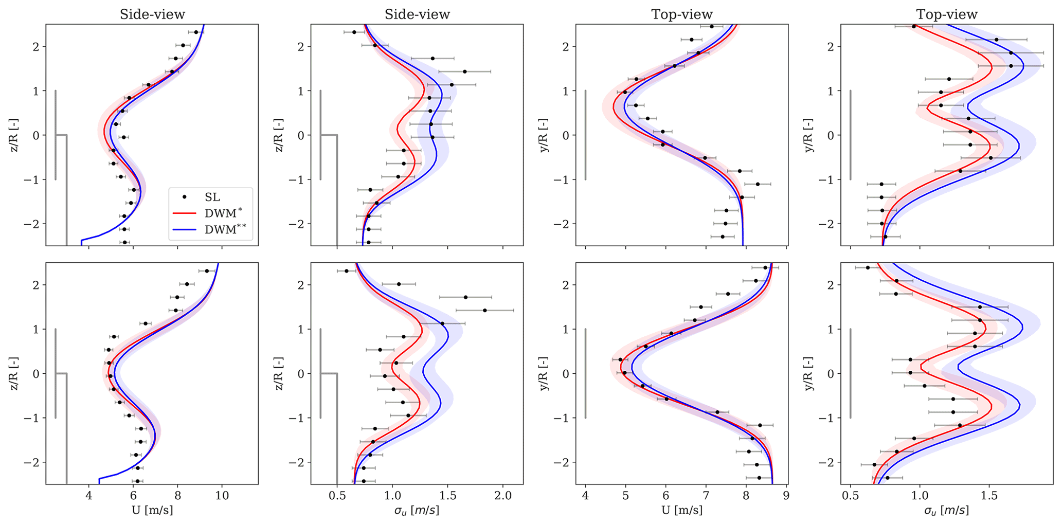
Figure 13 Comparisons between SpinnerLidar (SL)-measured and DWM-model-predicted spatial distribution of the mean and standard deviation velocity computed in the FFoR and obtained at 5 D in the wake region for two 10 min periods. The predictive DWM model that incorporates the SpinnerLidar-tracked meandering time series is denoted by DWM^* (red line), and that based on the meandering model complemented by measured inflow turbulence fluctuations from the mast and yaw offsets is denoted by DWM${}^{**}$ (blue line). The solid lines represent the mean predictions, whereas the shaded areas indicate the 95 % confidence intervals. The uncertainties in measurements are shown with error bars. The top view profiles are centred at hub height, whereas the side view profiles are centred along the vertical symmetry plane of the wake.

To evaluate the performance of the DWM model, we calculate two flow metrics that are relevant in aeroelastic simulations and compare them to relative measured quantities: the rotor-effective wind speed (U_eff), defined as the weighted sum of wind speeds across the rotor area, and the effective wake turbulence (σ_u, eff), which is derived as the weighted sum of turbulence estimates across the rotor. Figure 14 shows the one-to-one comparison between measured and DWM^*- and DWM${}^{**}$-model-predicted flow metrics for all 10 min periods. We find a slope that deviates <1 % from unity, with R²=0.95 for U_eff and a bias of ≈ 4 % and R²≈0.93 for σ_u, eff. The observed scatter is explained by the large measurement uncertainties, by the uncertainties in inflow wind parameters, and by those of the model predictions. The latter is estimated by propagating uncertainties in model parameters provided in Table 4, which result in a COV of 1 % for U_eff, and of 3 % for σ_u, eff. These findings indicate that the inferred uncertainties in model parameters do not propagate into an error of the same magnitude on the fully resolved wakes that are eventually input to aeroelastic simulations.

Further, a sensitivity analysis indicates that the variations in U_eff and σ_u, eff are mostly explained by the uncertainties in k₁ and k₂ and the wake tracking position $y_{\mathrm{m},\mathit{ϵ}},z_{\mathrm{m},\mathit{ϵ}}$; this is shown in Appendix B. The contribution of the wake-added turbulence from Eq. (17) to the total wake turbulence σ_u, eff in the FFoR is marginal and accounts for approximately 2 %–7 %. The turbulence induced by the meandering of the wake deficit is thus the major source of added turbulence (Madsen et al., 2010).

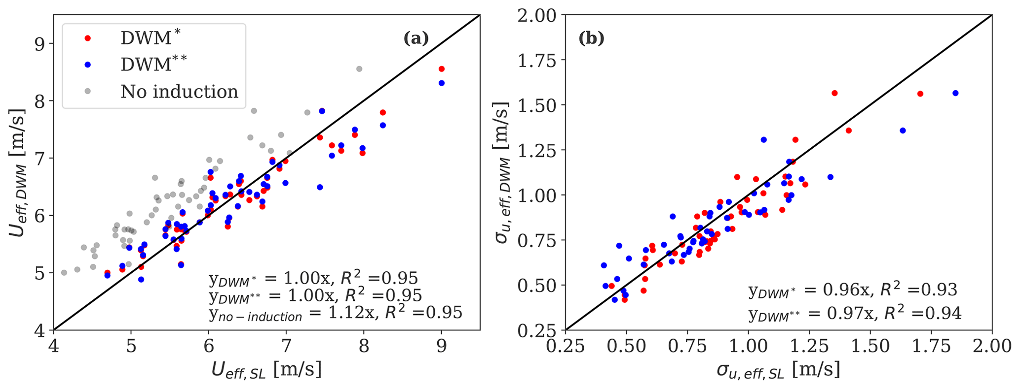
Figure 14 Comparison of the SpinnerLidar-measured (SL) and DWM-model-predicted rotor-effective wind speeds U_eff (a) and rotor-effective turbulence σ_u, eff (b). The DWM^* predictions (red markers) are obtained by constraining the meandering on the basis of SpinnerLidar-tracked wake displacements, while ${\mathrm{DWM}}^{**}$ uses mast-based meandering time series (blue markers). The SpinnerLidar U_eff statistics derived by neglecting induction effects are shown by grey markers (see Sect. 6.1 for more details).

7 Discussion

The SpinnerLidar measurements show that the wake recovers faster under unstable compared to stable conditions primarily due to the high turbulence levels of the former (Iungo et al., 2013; Zhan et al., 2020b). The wake recovery can be predicted accurately by the DWM model when using appropriate calibration parameters. Further, accurate reproduction of the wake meandering dynamics in both lateral and vertical directions is key for accurate wake simulations.

Although the SWiFT campaign provides a comprehensive dataset, including a wide range of inflow wind conditions and detailed two-dimensional lidar measurements of the wake field, the calibration parameters obtained from the 192 kW turbine with 32 m diameter should be further evaluated for multi-megawatt turbines with larger rotors. While this study cannot explicitly demonstrate the transferability of the obtained results for modern-size turbines, it highlights the need for datasets that include observations of the wake deficit profiles under varying stability conditions, inflow wind speeds, and downstream distances for the reliable and robust calibration of engineering wake models. Here, we find that the velocity deficit's recovery rate for increasing turbulence is the main difference among calibrations reported in the literature (see Fig. 9), which were based on either power production data (Larsen et al., 2013; IEC, 2019) or limited CFD simulations (Madsen et al., 2010; Keck et al., 2015) and one-dimensional observations of the wake field from a nacelle lidar (Reinwardt et al., 2020).

We also demonstrate that uncertainties in calibration parameters (e.g. COV${}_{k_{\mathrm{1}}}\approx \mathrm{21}$ % and COV${}_{k_{\mathrm{2}}}\approx \mathrm{19}$ %) do not lead to uncertainty of the same magnitude in the wind speed and turbulence fields (e.g. COV${}_{{\mathrm{U}}_{\mathrm{eff}}}\approx \mathrm{1}$ % and COV${}_{{\mathit{\sigma }}_{u,\mathrm{eff}}}\approx \mathrm{3}$ %) that are eventually used as input for the aeroelastic simulations. Note that the uncertainty in the simulated wake fields increases for increasing ambient turbulence due to the proportionality of k₁ to TI_amb in Eq. (1). Although a different dataset might produce other calibration parameters, it does not necessarily imply an improved accuracy of the simulated wake fields in the FFoR. Particularly, we expect our calibration and that of Madsen et al. (2010), Larsen et al. (2013), and IEC (2019) to provide similar wake fields in the FFoR for low ambient turbulence (i.e. ≤7 %), as illustrated by the blue lines in Fig. 9.

We recommend conducting DWM model calibrations using two-dimensional high-temporal- and high-spatial-resolution measurements of the wake field. Such resolution can be achieved by research-based nacelle lidars today, which allow the resolution of wake flow features including the wake deficit and wake-added turbulence profiles in the MFoR for model calibration. When using power production data for such calibrations (the IEC standard values are based on this approach), we are unable to distinguish between uncertainties from inaccurate wake deficit predictions and those from erroneous wake meandering representations. The latter play an important role in the accuracy of the fully resolved wake fields, which are inputs to aeroelastic simulations.

As wind turbines are typically spaced 5 D and beyond, it is recommended to focus future measurement campaigns and model validation studies on including those regions. Additional high-resolution datasets will allow a more comprehensive validation analysis to verify that the model proposed in this work is applicable for a wide range of conditions (e.g. turbine types and site conditions). To this extent, Bayesian inference is a valuable approach for updating the PDFs of model parameters estimated within this work by directly including data from future observations while retaining information from the earlier observations. Further, power and load validation analyses using the proposed calibration parameters at multiple sites can increase the confidence in our calibration methodology.

Characterizing wake turbulence using lidars is challenging due to the limited sampling frequency and probe volume effects (Peña et al., 2017). We demonstrate the usefulness of Doppler radial velocity spectra to compute unfiltered LOS variances in wake conditions. In addition to the enhanced turbulence intensity, the wake turbulence is characterized both by being highly isotropic and reduced turbulence length scale compared to the ambient turbulence (Madsen et al., 2005). These turbulence characteristics were not investigated in this work.

8 Conclusions

We analysed high-spatial- and high-temporal-resolution SpinnerLidar measurements of the wake field collected at the SWiFT facility and derived wake features such as the wake deficit, wake-added turbulence, and wake meandering under varying atmospheric-stability conditions, inflow wind speeds, and downstream distances. The SpinnerLidar-estimated wake characteristics computed in the MFoR were used to determine uncertainties in the DWM model parameters using Bayesian inference. The uncertainties in model parameters were propagated to predict fully resolved wake flow fields in the FFoR. This approach allowed us to quantify uncertainties in the DWM-model-simulated wake fields and to investigate the sensitivity of the model parameters to flow features that primarily affect power and load predictions.

The SpinnerLidar-derived wake deficit profiles revealed the strong impact of atmospheric stability on wake evolution. In particular, we observed the faster recovery of the deficit under unstable compared to stable regimes as higher turbulence intensities characterized the former. These effects were accurately reproduced by the eddy viscosity term of the DWM model with the inferred parameters for distances beyond 4 D. Our results indicate that the currently adopted parameters in the IEC standard lead to conservative velocity deficit predictions (up to 18 % for moderate to high ambient turbulence TI_amb≥12 %) at distances up to 5 D behind the rotor.

We proposed and verified an improved semi-empirical formulation of the wake-added turbulence model that captured the effects of the atmospheric shear and the ambient turbulence on the spatial re-distribution of the wake turbulence observed at 2.5 D. We also demonstrated that the wake meandering is the major source of added turbulence in the wake region.

The underlying hypothesis of the DWM model (i.e. wakes are advected passively by the large eddies in the incoming wind field) was verified by means of the SpinnerLidar-tracked meandering time series. The spectral analysis indicated that large eddies associated with sizes larger than 2 D are responsible for the wake meandering; however, the large-eddy “definition” had only marginal effects on the predicted wake fields. Accurate tracking of the wake centre position was the most influential factor in simulating wake flow fields accurately. We expect it to also play a central role in the accuracy of power and load predictions.

In a future study, we will quantify uncertainties in power and load predictions based on the proposed calibration at two different sites, the SWiFT facility and the Nørrekær Enge wind farm in Denmark (Conti et al., 2020b).

Appendix A: Comparisons of wake meandering time series

Figure A1 compares measured and predicted time series of the wake meandering in the lateral direction under varying stability conditions. The DWM model predictions are computed by applying the filtering cut-off frequency with the stochastic definition of the large-scale eddies (D_m). A reasonable agreement between the two signals is found, where the major wake displacements are captured by the meandering model. Note that improved correlation can be achieved by utilizing a reduced advection wind speed in the time-lag parameter in Eq. (4) compared to the ambient wind velocity. Nevertheless, the largest observed movements are induced by the yawing of the WTGa1, which is fairly frequent within the analysed dataset. Further, the 95 % confidence interval of the meandering predictions obtained by propagating uncertainties in the D_m definition is nearly negligible. This indicates that uncertainties in the filtering cut-off frequency used in the DWM model formulation have a marginal effect on the accuracy of wake simulations.

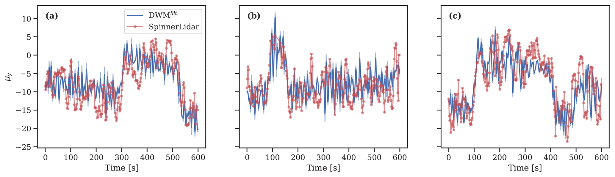
Figure A1 Time series of the wake meandering in the lateral direction observed by the SpinnerLidar (red markers) and those derived from the meandering model of Eq. (4) denoted as DWM^filt. (blue lines) under stable (a), near-neutral (b), and unstable conditions (c). The predictions are obtained at 2.5 D behind the rotor. The shaded blue areas indicate the 95 % confidence intervals obtained by propagating the uncertainty in the large-scale-eddy definition

Appendix B: Sobol sensitivity indices

Sensitivity analysis is conducted to identify the most important parameters affecting the accuracy of wake simulations. Here, we only investigate the uncertainties in the model parameters, which are listed in Table 4, and assume that the inflow conditions are perfectly prescribed. We employ a variance-based sensitivity method and compute total Sobol indices (Sobol, 2001; Saltelli et al., 2010). The Sobol sensitivity decomposes the variance of the response (e.g. U_eff and σ_U, eff) into contributions from input parameters and associated interactions.

The Sobol indices computed from wake simulations at five rotor diameters behind the rotor are illustrated in Fig. B1. Note that uncertainties in wake centre locations (y_m, ϵ and z_m, ϵ) have a similar influence as for the calibration parameters (i.e. k₁ and k₂) on the predicted flow features such as U_eff and σ_u, eff. Overall, tracking the wake meandering in both lateral and vertical directions is of primary importance in wake field representations and therefore in power and load validations. The sensitivity of the wake-added turbulence model parameters as well as the large-scale-eddy definition (D_m) is marginal. It is inferred that these parameters can be considered to be deterministic without compromising the accuracy of wake simulations.

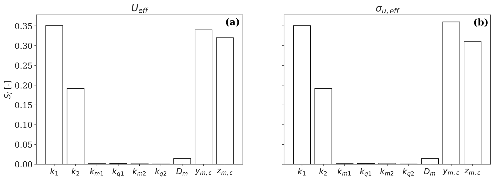
Figure B1 Variance decomposition (Sobol indices) for the rotor-effective wind speed (a) and a measure of the rotor-effective turbulence (b).