Satellite-based estimation of roughness lengths and displacement heights for wind resource modelling

Wind turbines in northern Europe are frequently placed in forests, which sets new wind resource modelling requirements. Accurate mapping of the land surface can be challenging at forested sites due to sudden transitions between patches with very different aerodynamic properties, e.g. tall trees, clearings, and lakes. Tree growth and deforestation can lead to temporal changes of the forest. Global or pan-European land cover data sets fail to resolve these forest properties, aerial lidar campaigns are costly and infrequent, and manual digitization is labour-intensive and subjective. Here, we investigate the potential of using satellite observations to characterize the land surface in connection with wind energy flow modelling using the Wind Atlas Analysis and Application Program (WAsP). Collocated maps of the land cover, tree height, and leaf area index (LAI) are generated based on observations from the Sentinel-1 and Sentinel-2 missions combined with the Ice, Cloud, and Land Elevation Satellite-2 (ICESat-2). Three different forest canopy models are applied to convert these maps to roughness lengths and displacement heights. We introduce new functionalities for WAsP, which can process detailed land cover maps containing both roughness lengths and displacement heights. Validation is carried out through cross-prediction analyses at eight well-instrumented sites in various landscapes where measurements at one mast are used to predict wind resources at another nearby mast. The use of novel satellite-based input maps in combination with a canopy model leads to lower cross-prediction errors of the wind power density (rms = 10.9 %–11.2 %) than using standard global or pan-European land cover data sets for land surface parameterization (rms = 14.2 %–19.7 %). Differences in the cross-predictions resulting from the three different canopy models are minor. The satellite-based maps show cross-prediction errors close to those obtained from aerial lidar scans and manually digitized maps. The results demonstrate the value of using detailed satellite-based land cover maps for micro-scale flow modelling.

1 Introduction

Wind turbines on land represent a cost-competitive source of renewable energy (Global Wind Energy Council, 2019). More than 95 % of the global installed wind energy capacity of ≈733 GW in 2020 is installed on land (https://www.irena.org/wind, last access: 21 April 2021). In northern Europe's temperate climates, a vast amount of the land surface is covered by forest. The exploitation of wind power within such forests has become more widespread as the hub height of modern wind turbines has exceeded the forest height (Enevoldsen, 2016).

Wind resource assessment is typically performed with linearized modelling in a wind farm siting tool (e.g. WAsP or WindPRO), which contains several submodels to predict the flow based on an input wind histogram (Troen and Petersen, 1989). Based on Monin–Obukhov similarity theory (Eq. 1), the flow model can be used to predict the wind speed, U, for any height, z, above the ground:

$$\begin{array}{}\text{(1)}& U={\displaystyle \frac{u_{*}}{\mathit{\kappa }}}\left[\ln {\displaystyle \frac{z-d}{z_{\mathrm{0}}}}-{\mathrm{\Psi }}_m\right],\end{array}$$

where u_* is the friction velocity, κ is the von Kármán constant (=0.4), z₀ is the aerodynamic roughness length, and Ψ_m represents the stability correction to the profile and depends on $z/L$, where L is the Monin–Obukhov length (Businger et al., 1971). In addition to z₀, the zero-plane displacement height, d, is traditionally used at forested sites to account for the canopy, forcing the mean flow to be displaced upwards over forests (Thom, 1971). A dense forest appears more smooth (i.e. a lower z₀) and has a larger d than a sparse forest with clearings (Shaw and Pereira, 1982).

Values of z₀ and d can be assessed through visual inspection of the forest at a given site combined with digital maps. In practice, a background value for z₀ and d is set, and adjustments are made for specific areas where the roughness and displacement height differ from the background values. Manual assessments are subjective and time-consuming, and they can lead to a high level of uncertainty of the estimated wind resource (Kelly and Jørgensen, 2017).

Fully automated assessments of z₀ and d can be achieved based on global or regional land cover data sets derived from satellite observations. Each land cover class is assigned a value of z₀ and d via a land cover table (Jancewicz and Szymanowski, 2017; Floors et al., 2018). State-of-the-art flow modelling tools offer embedded access to such land cover maps and to the associated roughness translation tables, which the user may modify. Due to the coarse spatial resolution of global land cover data sets (grid spacing of 100–1000 m), the finer-scale variability within a forest, such as smaller clearings on the order of 10–100 m, is not resolved. Further, the available land cover-to-roughness translation tables may not be fully representative for the site in question due to the data sets' global nature. For example, commonly used tables (see Appendix A) show very low roughness lengths for forest classes, which might not be accurate for areas with heterogeneously forested land cover (Floors et al., 2018).

Enevoldsen (2017) and Floors et al. (2018) have demonstrated that tree heights and forest densities retrieved from aerial lidar scans can be used to parameterize z₀ and d over the forest. This approach is more physical than the ad hoc assignment using land cover data sets. It sets new requirements to the flow modelling tools used for wind energy siting because (i) a canopy model is needed to estimate z₀ and d from the tree height and density, and (ii) the data processing routines in the flow modelling tool need to be more efficient due to the finer resolution of z₀ and d that result from lidar-derived canopy measurements. Several countries in northern Europe have released national aerial lidar scans, and in addition, dedicated aerial lidar campaigns may be carried out to obtain location-specific data sets for wind farm planning. Lidar campaigns are rare due to the high cost of the instrumentation and deployment and the time-intensive data processing requirements. The temporal frequency of such observations is therefore low.

A wealth of new satellite observations with unprecedented spectral properties and spatial and temporal resolutions have become available, e.g. through Copernicus (https://www.copernicus.eu, last access: 27 September 2021). Forest monitoring is a key objective of several new missions because information on deforestation and forest degradation is important in connection with climate change mitigation. However, key metrics for wind-resource assessment such as the forestry canopy height are still missing or only available at a low spatial resolution, but they can be derived through post-processing of the data from available sensors. Here, we hypothesize that such post-processed values of the forest canopy height and density retrieved from satellites at a high spatial resolution can also be used to estimate the wind resource for a site with the same accuracy as aerial lidar scans but at a lower cost.

This paper uses tree heights and densities retrieved from satellite observations to derive roughness lengths and displacement heights that are then used to estimate the wind energy resource available at forested sites. Based on wind observations from meteorological masts at eight sites worldwide, we evaluate the prediction errors on the wind power density and the mean wind speed, and we compare them with predictions based on global land cover maps, aerial lidar scans, and manual digitization for the parameterization of z₀ and d.

2 Background

2.1 Forest parameters from satellites

Firstly, a goal in this paper is to derive tree heights from satellites. The Ice, Cloud, and Land Elevation Satellite-2 (ICESat-2) carries the Advanced Topographic Laser Altimeter System (ATLAS), used to observe the land surface height with great precision. Amongst many other parameters, the mission delivers global forest canopy heights (Neuenschwander and Pitts, 2019), which are well correlated with canopy heights from aerial lidar scans (Li et al., 2020) and field measurements (Huang et al., 2019). A mission with similar capabilities to ICESat-2 is the Global Ecosystem Dynamics Investigation (GEDI). However, GEDI only collects data up to 52^∘ north and south of the Equator and therefore does not offer global coverage. Although representing a major advancement in estimating 3D forest structure, these current spaceborne laser observations are restricted to very narrow footprints, which are insufficient to map canopy heights over larger areas. Recent studies have shown that the laser-derived canopy heights can be extrapolated through different combinations with other satellite observations and machine learning techniques (Csillik et al., 2020; Fagua et al., 2019). Typically, the canopy heights from laser measurements are extrapolated using textural information from active microwave sensors (e.g. Sentinel-1 or ALOS PALSAR) and multispectral information from passive sensors (e.g. Landsat or Sentinel-2) (Li et al., 2020).

Secondly, in connection with flow modelling for wind energy, the leaf area index (LAI) can be used as a proxy for the forest density (Raupach, 1994). LAI is defined as the one-sided green leaf area per unit ground area in broadleaf canopies and as one-half the total needle surface area per unit ground area in coniferous canopies (Chen and Black, 1992). Several space-borne sensors, operating in the visible and near-infrared range, monitor LAI and other vegetation properties daily. For example, the Terra and Aqua satellites each carry a Moderate Resolution Imaging Spectroradiometer (MODIS). From the two instruments in combination, 4 d composites of LAI are generated routinely. This product has a relatively coarse resolution and a pixel size of 500 m. Guzinski and Nieto (2019) have developed a method for downscaling of LAI estimates.

2.2 Forest roughness models

Different models can be used to estimate z₀ and d from forest canopy heights and LAI. Here, we consider the objective roughness approach (ORA), the Raupach model, and the scalar distribution (SCADIS) model.

2.2.1 The objective roughness approach (ORA)

The relation between the canopy height, h, and z₀ and d has been recognized and discussed by many authors (Thom, 1971; De Bruin and Moore, 1985; Enevoldsen, 2017). Because z₀ is usually proportional to h, an easy way to obtain z₀ and d is by relating them linearly to the canopy height,

$$\begin{array}{}\text{(2)}& z_{\mathrm{0}}=c_{\mathrm{1}}h,\end{array}$$

and

$$\begin{array}{}\text{(3)}& d=c_{\mathrm{2}}h.\end{array}$$

Maps based on lidar scans using the constant values c₁=0.1 and $c_{\mathrm{2}}=\mathrm{2}/\mathrm{3}$ were shown in Floors et al. (2018) to reduce the risk of making large errors (>25 %) in predicted power density by 40 %–50 % compared to the best land cover database at a forested site.

2.2.2 The Raupach model

Raupach (1992) developed a model to predict the bulk drag coefficient over a rough surface with a given canopy height. The main model parameter resulting from his analysis is the frontal area index λ, which for isotropically oriented elements is given by

$$\begin{array}{}\text{(4)}& \mathit{\lambda }=\mathrm{0.5}\text{LAI}.\end{array}$$

Raupach (1994) discussed some simplifications to the original model and suggested

$$\begin{array}{}\text{(5)}& {\displaystyle \frac{d}{h}}=\mathrm{1}-b,\end{array}$$

where

$$\begin{array}{}\text{(6)}& b=\mathrm{1}-{\displaystyle \frac{\exp (-a)}{a}}\end{array}$$

and

$$\begin{array}{}\text{(7)}& a=\sqrt{\mathrm{2}{c}_{d\mathrm{1}}\mathit{\lambda }}.\end{array}$$

c_d1 was experimentally found to be equal to 7.5. Finally, the roughness length is estimated as

$$\begin{array}{}\text{(8)}& {\displaystyle \frac{z_{\mathrm{0}}}{h}}=b\exp \left({\displaystyle \frac{-\mathit{\kappa }}{min\left(\sqrt{C_S+C_R\mathit{\lambda }},c_{max}\right)}}-{\mathrm{\Psi }}_h\right).\end{array}$$

Raupach (1994) suggested based on empirical evidence that C_S=0.003, C_R=0.3, $c_{max}=\mathrm{0.3}$, and Ψ_h=0.193.

2.2.3 The SCADIS model

A criticism of the Raupach (1994) model is that some of the constants are highly dependent on the structure of the canopy and may not be universally applicable. To address this, one can use a one-dimensional version of a k–ω turbulence model, which depends on the leaf area density profile within the canopy (Sogachev et al., 2002; Sogachev and Panferov, 2006). An additional advantage of this model is that it can estimate z₀ and d in non-neutral atmospheric conditions.

The leaf area density (LAD) profile is frequently described (e.g. Meyers and Tha Paw U, 1986) by a beta probability density function,

$$\begin{array}{}\text{(9)}& \text{LAD}=\text{LAI}\left[(z/h{)}^{\mathit{\alpha }-\mathrm{1}}(\mathrm{1}-z/h{)}^{\mathit{\beta }-\mathrm{1}}\right],\end{array}$$

where α=9 and β=3. The chosen constants are representative of a temperate pine forest, and we use them throughout this work due to the absence of information on the canopy profile from satellite data. Sogachev et al. (2017) validated the SCADIS model for flow over a 3D area with forested terrain and found that simulations that explicitly resolve the drag of the canopy and those that use an effective z₀ compare well.

2.3 Flow modelling and cross-prediction

Maps of z₀ and d can be used in combination with terrain elevation maps as input to wind energy flow models. The WAsP methodology (Troen and Petersen, 1989) can be applied to analyse the observed wind climate (a histogram of wind speeds for each wind direction sector) at a particular mast location and height and predict the wind climate at a nearby location, assuming the same large-scale atmospheric forcing. The effects of land surface roughness and orography are first removed from the observed wind climate. Equation (1) and the geostrophic drag law (Blackadar and Tennekes, 1968) are then used to estimate the geostrophic wind speed distribution, which is assumed to be valid some kilometres away from the mast. The geostrophic wind speed distributions can be transformed to Weibull distributions over idealized flat terrain at a number of specified heights and z₀ (see Sect. 8.7 in Troen and Petersen, 1989). The result of this process is a so-called generalized wind climate (GWC), which is characterized by the Weibull parameters A and k and the probability density per wind direction sector. The GWC can be used to predict the wind resource near the measurement site by adding local roughness and orographic speed-up factors. The process of predicting the wind climate from one position to another is called a cross-prediction. The accuracy of such predictions depends strongly on the quality of the roughness and elevation maps used as input (Floors et al., 2018).

3 Sites and data

In this section, we present eight sites that are considered in this study and the different types of input data which are needed for cross-prediction analyses at the sites.

3.1 Measurement sites

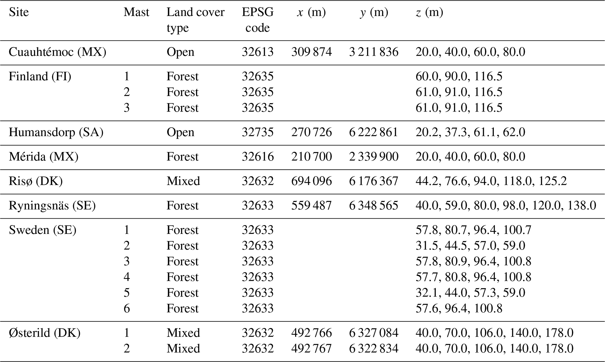
Eight measurement sites are selected for cross-prediction analyses (Table 1). The sites represent vastly different land cover types and complexities. The sites Ryningsnäs, Finland, and Sweden are located in forests, where the displacement height becomes important, and the uncertainty in wind resource assessment is known to be high (Kelly and Jørgensen, 2017). The site near Mérida has low (h≈5 m) and irregular forest in all directions. The sites Cuauhtémoc and Humansdorp are surrounded by very open landscapes where the WAsP model is expected to perform well. The sites Risø (Giebel and Gryning, 2004) and Østerild (Peña, 2019) are characterized by a mixture of forest and open areas near the mast, which is more challenging in terms of flow modelling. The sites in Sweden and Finland are from confidential projects, and the exact locations of these can therefore not be disclosed.

Table 1 Sites and masts used for cross-prediction analyses. The characteristic land cover is indicated. The EPSG code identifies the coordinate reference system, including the map projection, datum, and zone number (see text), and the x, y, and z columns identify the positions in projected map coordinates.

3.2 Surface roughness maps

3.2.1 Standard land cover data sets

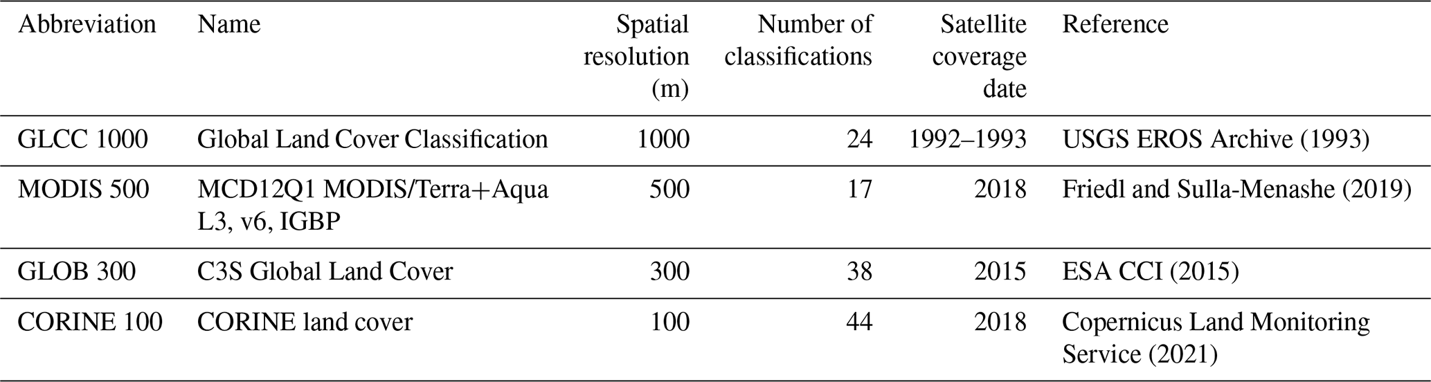
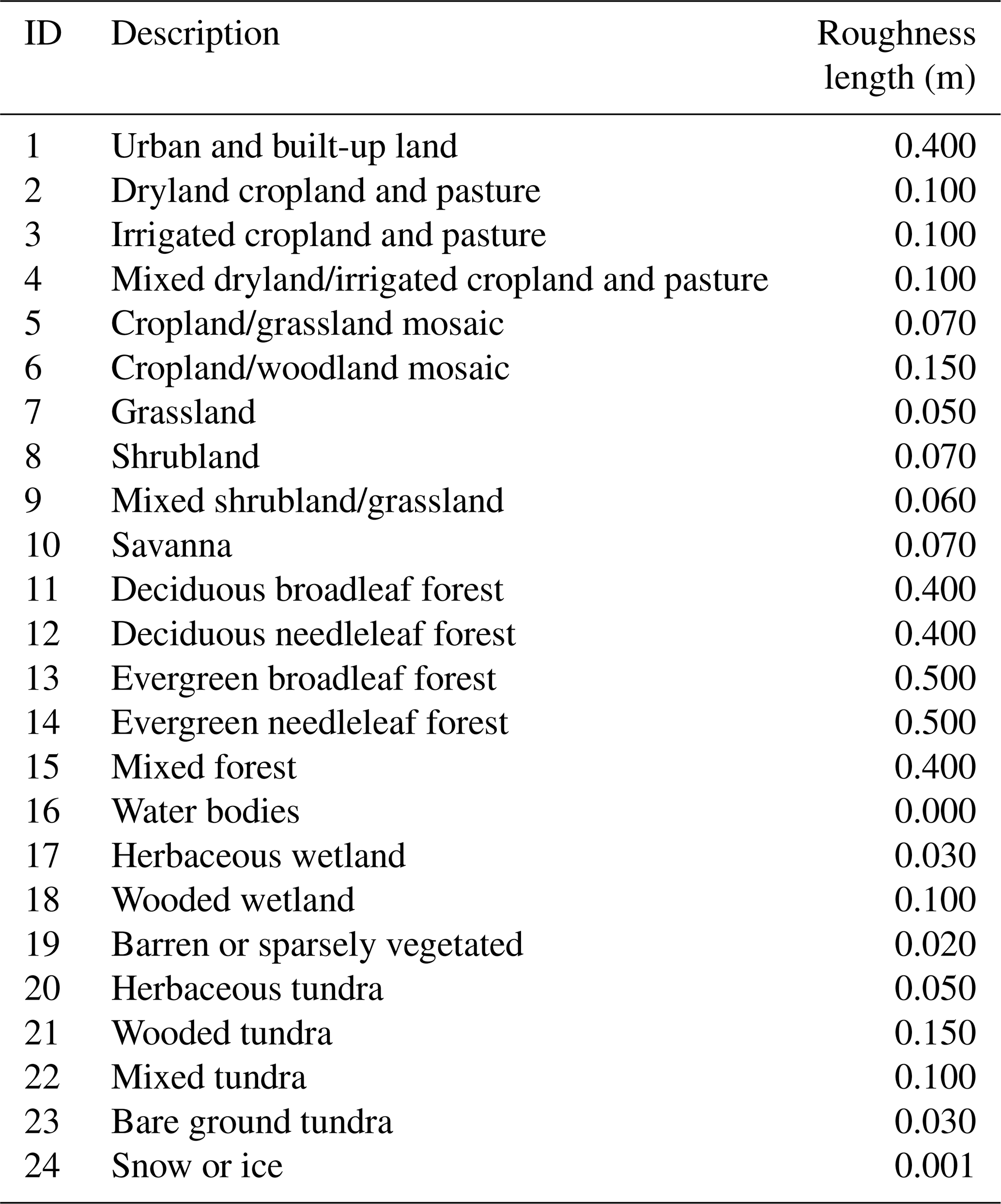
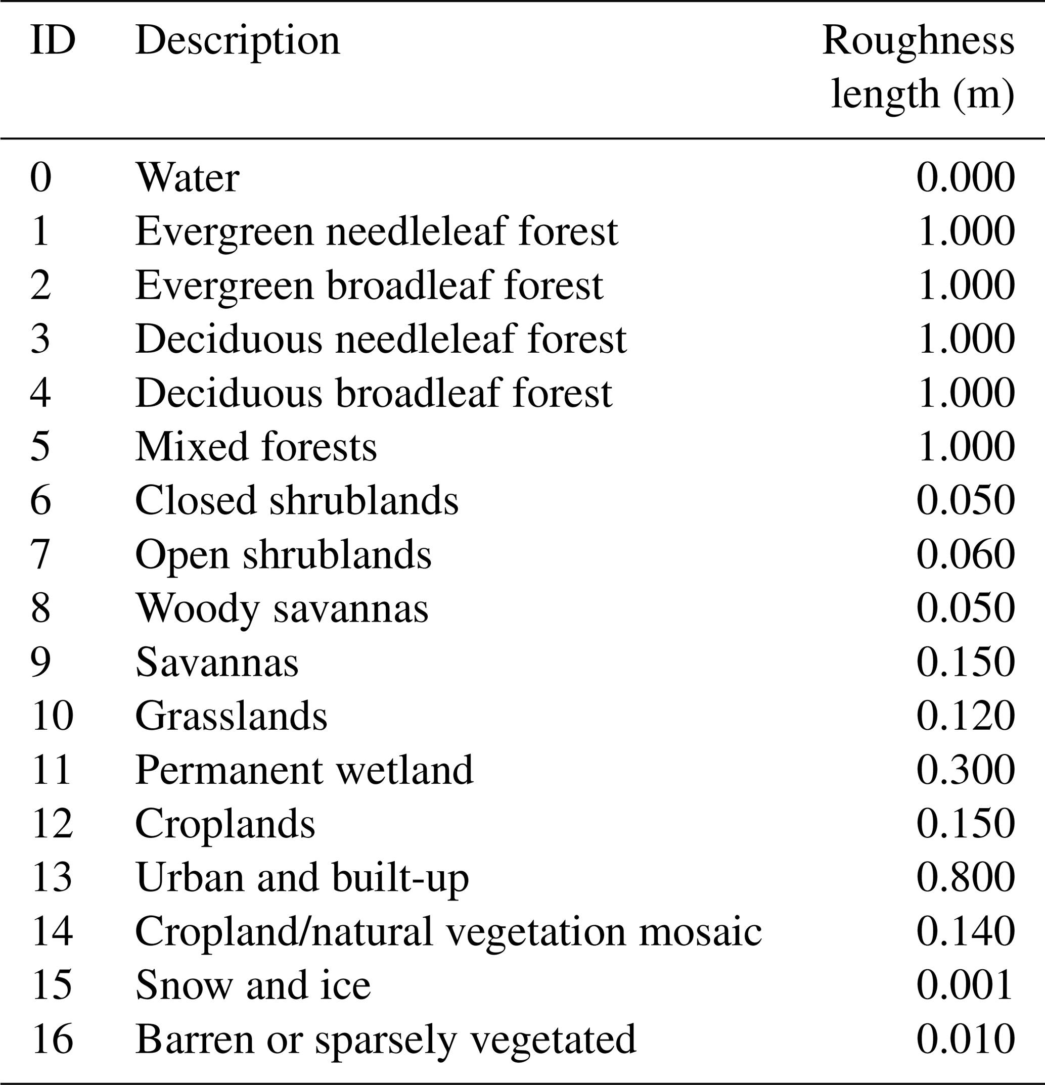
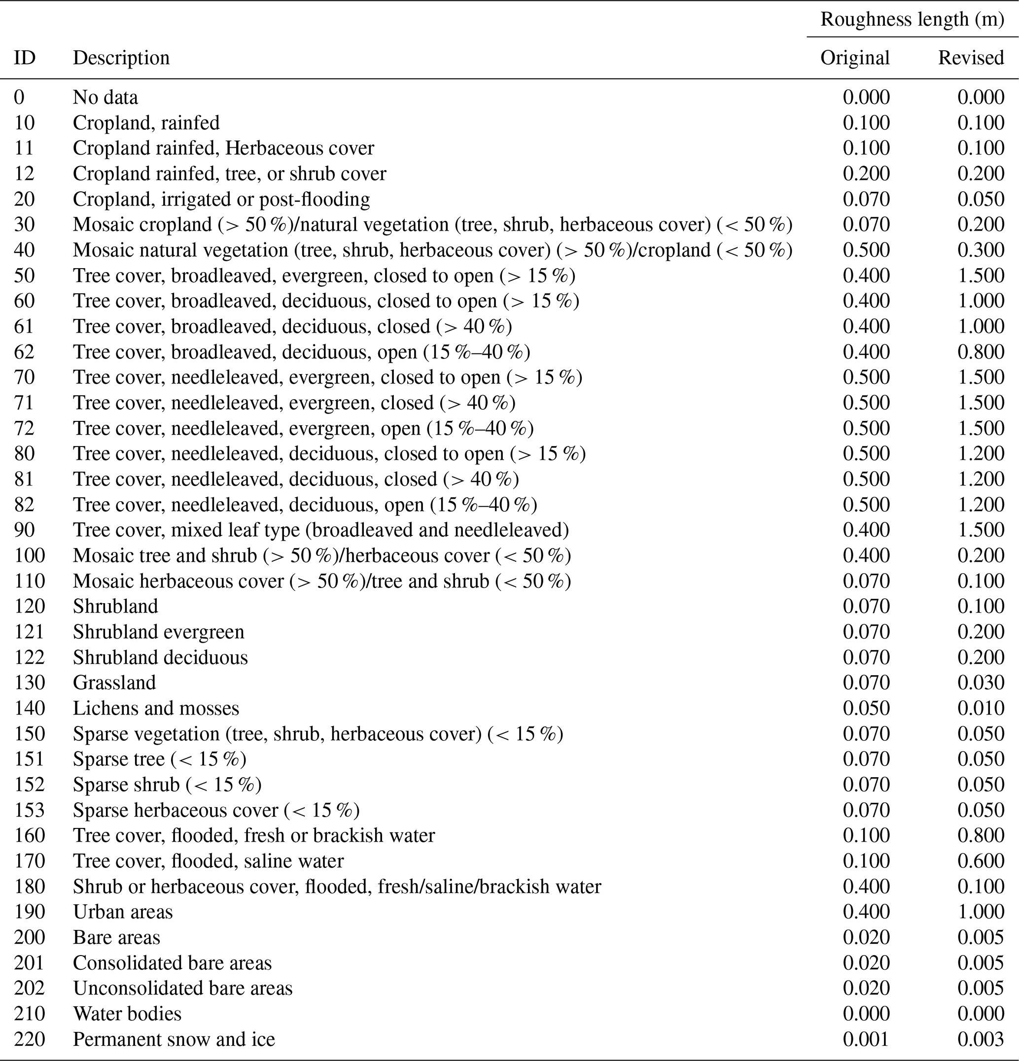
Four coarse-resolution land cover databases (spatial discretization between 100 and 1000 m) that are regularly applied for wind energy modelling are used in connection with this analysis. These are the Global Land Cover Characterization (GLCC 1000), the MODIS MCD12Q1 V6 product (MODIS 500), the C3S Global Land Cover product (GLOB 300), and for the European sites the Corine Land Cover inventory (CORINE 100). Further details about the land cover products are given in Table 2.

USGS EROS Archive (1993)Friedl and Sulla-Menashe (2019)ESA CCI (2015)2021

Table 2 Summary of the different coarse-resolution land cover products (spatial discretization between 100 and 1000 m) used for creating the roughness maps.

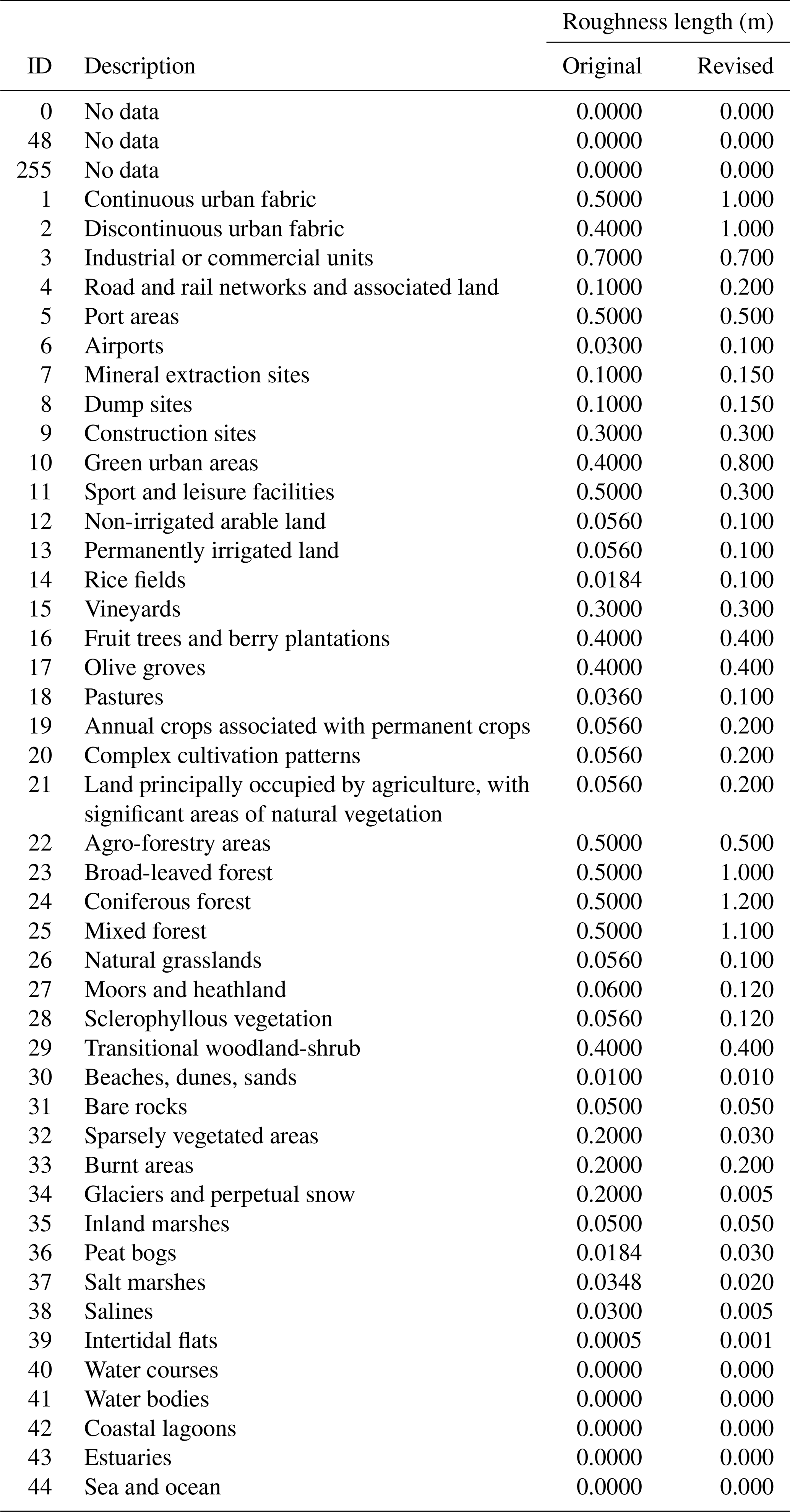
The coarse-resolution land cover data sets come with standard roughness conversion tables (Appendix A, Tables A1–A5). The z₀ for forest classes tends to be too low for temperate forests (Floors et al., 2018). Recent studies of Dörenkämper et al. (2020) and Badger et al. (2015) have highlighted this shortcoming and have suggested higher z₀ for forested areas. To reflect the uncertainty of z₀ assignments in forested areas, we include the original vs. revised values in Tables A1–A5. In connection with the C3S Global Land Cover product, the z₀ classification is based on the data set of 2009, and some of the 23 land cover classes have been split into sub-classes since then. Therefore, z₀ of each subclass is assumed to be identical to z₀ of the class it inherits from (see Table A3). It is mostly classes with forests that have been split up, and one could get a better estimation of z₀ by a more detailed analysis of the canopy structure in these subclasses. However, this approach is not attempted here.

3.2.2 Novel Sentinel data sets

High-resolution satellite-based data packages are developed for an area of 40×40 km around each of the eight sites described above. Each data package has a regular grid spacing of 20×20 m and includes (1) land cover classification, (2) LAI, and (3) forest canopy height. These data are derived from satellite imagery using machine learning methods. Specifically, random forests (Breiman, 1996) are used to classify land cover and for down-scaling LAI, while support vector machines (Boser et al., 1992) are used for canopy height estimation. Both algorithms are from a family of supervised machine learning methods that are routinely applied to satellite imagery to extract features of interest. This is done by supplying the algorithms with a set of samples from the satellite imagery that have known labels (e.g. land cover class or canopy height). These samples are used to train the machine learning models whereby the algorithms learn to predict each feature of interest across the entire satellite image. The primary data source used for the production of the three data layers is Copernicus satellite imagery from the Sentinel-1 and Sentinel-2 missions. Sentinel-1 is a c-band (5.6 cm) synthetic aperture radar sensor, while Sentinel-2 is an optical sensor providing data in the visible, near-infrared, and shortwave infrared parts of the spectrum.

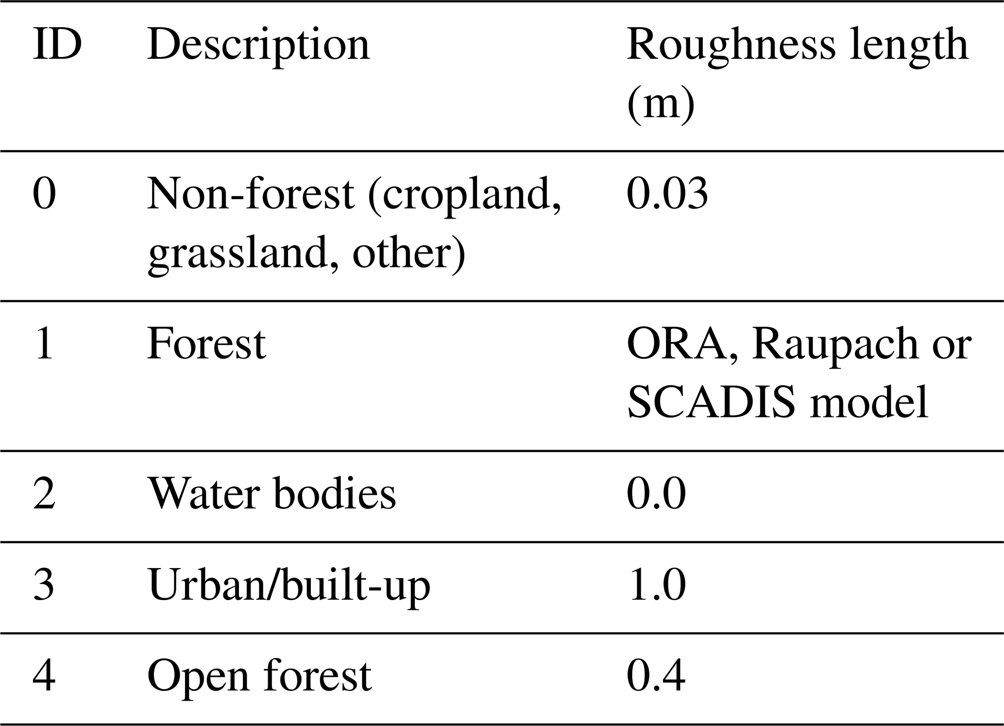
The land cover classification is based on five land cover classes most relevant for wind modelling (Appendix A, Table A5). For each site, training data are collected for each land cover class by manually labelling areas in satellite imagery of known land cover. These training data are used as a dependent variable in a random forest model to predict land cover for each 20×20 m grid cell. Independent variables used for the land cover classification model include observations from the Sentinel-1 and Sentinel-2 sensors. LAI has been estimated for all grid cells identified as forest in the land cover classification through down-scaling of coarse-resolution LAI from the MODIS sensor to the 20×20 m grid of the Sentinel-2 observations (Guzinski and Nieto, 2019).

Forest canopy heights are estimated for all grid cells identified as forest in the land cover classification. Canopy height estimates from the ICESat-2 sensor are used as a dependent variable to train a support vector regression model to predict forest canopy height for each 20×20 m grid cell. Observations from Sentinel-1 and Sentinel-2 are used as independent variables in the regression model. ICESat-2 provides a globally available data set from the US National Aeronautics and Space Administration (NASA) that uses space-borne lidar technology to estimate ground and vegetation heights. It does this with six laser beams, scanning a swath of terrain 9 km wide, with each beam having a footprint of 17 m diameter. Because of the Sentinel sensors' importance for obtaining the three layers described above, they are labelled “Sentinel” throughout the rest of this paper.

3.2.3 Reference data sets

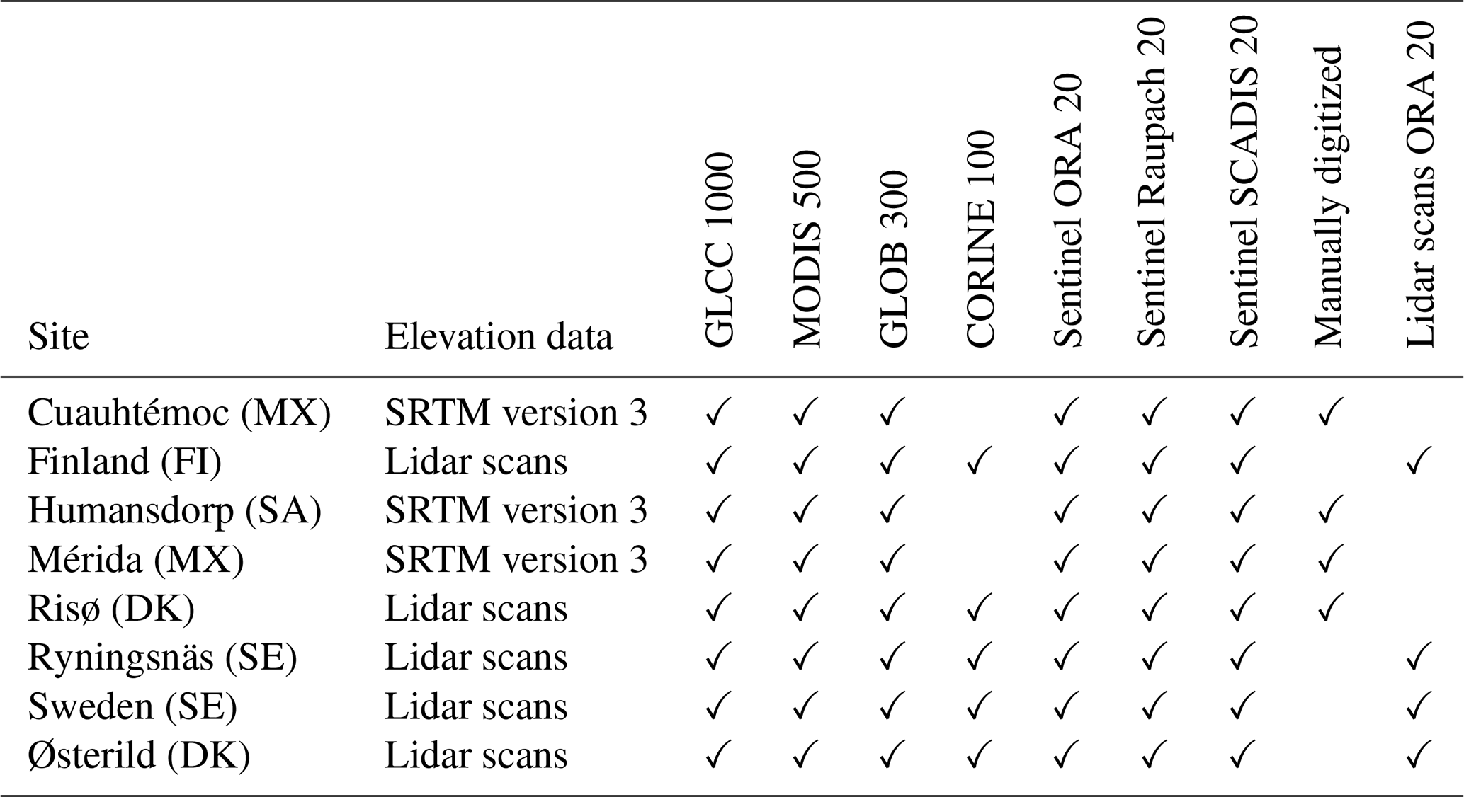
To validate the novel Sentinel maps, we consider two types of roughness maps for reference: (1) from manual digitization and (2) from lidar scans for sites where such data are readily available from previous works. For an experienced wind resource engineer, the most accurate way to obtain a land cover data set is by visual inspection in the field or using photographs followed by digitization of the land cover areas with the biggest impact on the flow. A representative z₀ is then assigned to each of these areas. Maps digitized manually are available for Cuauhtémoc, Humansdorp, Mérida, and Risø (see Table 3). Another approach to obtain an accurate roughness map is by using lidar scans. Tree heights can be retrieved from the cloud point data delivered by airborne lidars. The lidar data sets are described further in Sect. 3.3 as they are also used to map the terrain elevation. Once h is obtained from lidar scans, the procedure described in Sect. 3.2.1 in Floors et al. (2018) is used to estimate z₀ and d for Ryningsnäs, Sweden, and Østerild. The reference maps are denoted as “manually digitized or lidar scans” throughout the rest of the paper (see Table 3).

Table 3 Overview of the input data that are used for each site to estimate wind resources. The meaning of the different abbreviations are discussed in the text.

3.3 Elevation maps

In addition to the land surface roughness, a flow model needs inputs of the terrain elevation. Lidar scans can be used to retrieve the terrain elevation and also to estimate the canopy height at forested sites as described above (Popescu et al., 2003; Floors et al., 2018). Elevation data from aerial lidar scans are available for five of the eight sites analysed here (Table 3). The Swedish sites are covered by a national laser campaign conducted in 2013 (Lantmäteriet, 2021). The retrieved elevation data are available with a 20×20 m grid spacing. Lidar scans are available for the Danish site Østerild at the same spatial resolution, whereas the Finland elevation model is a digital terrain model produced by the National Land Survey of Finland (Maanmittauslaitos, MML) and available at a 10×10 m grid. For Risø, elevation data are obtained from the 2.5 m contour lines from “Danmarks Højdemodel” (Styrelsen for Dataforsyning og Effektivisering, 2016).

Elevation data for the two Mexican sites, Cuauhtémoc and Mérida, and the site in South Africa, Humansdorp, are obtained from the Shuttle Radar Topography Mission (NASA JPL, 2013) at 90 m resolution. We note that wind engineers should be careful when using databases such as SRTM in combination with a displacement height. Because the SRTM product shows the height of the surface, it includes the tree height. If this is not taken into account, the turbine or mast might be placed at too high elevation, and there is a risk of double-counting of the effects of the forest.

4 Methodology

The WAsP model is a microscale flow model that is frequently employed for wind resource assessments (Troen and Petersen, 1989). It contains submodels for orography, roughness changes, obstacles, and stability effects. In the following, we explain how the roughness and orographic submodels within WAsP are modified to better utilize the high spatial detail of z₀ and d obtained from the Sentinel data set. We then describe the cross-prediction method that is applied to test the novel Sentinel data sets against more conventional input data for wind energy flow modelling.

4.1 Model setup

The WAsP model consists of a graphical user interface and a core model that is written in the programming language Fortran. In the following, we refer to the core model code that is directly accessed via a set of Python codes. The routines are not yet available in the graphical user interface, but a new WAsP version scheduled for release in late 2021 will include them. One of the main advantages of the WAsP core model is its speed: it typically takes seconds to calculate the annual energy production (AEP). The newly implemented routines are parallelized using OpenMP in the Fortran language. Because in the WAsP core each grid point is independently calculated, the problem is easily distributed across central processing units. The standard settings of the WAsP core model (corresponding to WAsP version 12.6) are used here unless otherwise specified. In the following, we describe the modifications to the roughness and orographic submodules. The different parts of the model chain described in this section are shown in Fig. 1.

Figure 1 Process diagram of the submodels in WAsP. The rounded rectangles denote data structures, and the square boxes denote a method.

4.1.1 Forest submodel

The ORA and Raupach models are used to obtain z₀ and d and were implemented as described in Sect. 2.2. The SCADIS model is run without Coriolis force, because we want to obtain z₀ and d for the logarithmic wind profile in the surface layer. The height of the model domain is specified as 4h. The height of the first model level is specified to be z₁=0.5z_0b, where the background roughness length z_0b=0.3 m. The SCADIS model is run from an initial logarithmic profile (z₀=z_0b) with a wind speed of 10 m s⁻¹ at the domain top. The time step in the model is set to 300 s. The model integration is terminated when the wind speed at the canopy top changes less than 0.001 m s⁻¹. Finally, z₀ and d are then found by fitting $\frac{\mathrm{d}U}{\mathrm{d}z}=\frac{u_{*}}{\mathit{\kappa }(z-D)}$ to U and u_* obtained in the range from 1.5h to 2.5h.

4.1.2 Roughness submodel

Previous versions of WAsP use an algorithm, which finds all z₀ crossings between the roughness lines defined in a map and a number of rays extending from the point of interest. In this study we are not only interested in z₀ of a land cover patch, but we also want to take into account the effect of a displacement height, d. This information has to be passed from the land cover contour lines to the roughness model. The roughness submodel in WAsP uses vector lines as input, and therefore, the satellite-based raster maps of land cover are first converted to a vector-map format.

The new routines expect the input of “identifier” lines; i.e. each line contains an identifier (ID), which represents a certain land cover left and right of the line. This ID is then represented in a land cover table, which prescribes the corresponding z₀, d, and a description of that land cover class (Appendix A, Tables A1–A5). Keeping the land cover table separate from the map has several advantages, like the possibility to perform sensitivity studies with respect to z₀ and d, which has been difficult so far because one has to modify the contour map itself in an external program.

Using the approach above, we can process the standard land cover maps (see Sect. 3.2.1). The novel Sentinel maps contain additional layers with h and LAI. h is discretized into bins of 5 m and the LAI into bins of 1. The result is a Sentinel land cover raster map which typically contains 10–40 different classes of forest types plus the classes specified in Table A5.

For the forest class the centre of the h and LAI bins are used to estimate z₀ and d according to the three roughness models described in Sect. 2.2. Because the forest submodel operates on a table and not on the contour lines in the map itself, the conversion of h and LAI to z₀ and d is fast (i.e. the speed of the computation scales with the number of entries in the land cover table).

In order to introduce land cover, a new routine, here referred to as a “spider grid analysis”, is developed. It uses a polar zooming grid, similarly to the orographic flow model (Troen, 1990). The advantage of using a zooming grid is that it concentrates the resolution where it is most needed, and we can use arbitrarily distributed points. The latter is for example beneficial for calculating the wind climate at exact positions of wind turbines. The distance to the first radial segment r₀ in the zooming grid is defined by the user (default r₀=25 m), and each next segment has a grid spacing that is 5 % larger than the previous one. The number of azimuthal bins (i.e. wind direction sectors) can also be specified by the user and by default is set to 12, i.e. using a sector width of 30^∘. The first sector is always centred at the north.

For each cell in the zooming grid, the fraction of the total area f_i that each of a total of N land cover types in the land cover table occupies is determined, and the roughness length is calculated,

$$\begin{array}{}\text{(10)}& \ln z_{\mathrm{0}}=\sum _{i=\mathrm{1}}^N{f}_i\ln z_{\mathrm{0}i}.\end{array}$$

The displacement height is taken into account similarly to z₀ and is calculated for each cell in the zooming grid as

$$\begin{array}{}\text{(11)}& d=\sum _{i=\mathrm{1}}^N{f}_i{d}_i.\end{array}$$

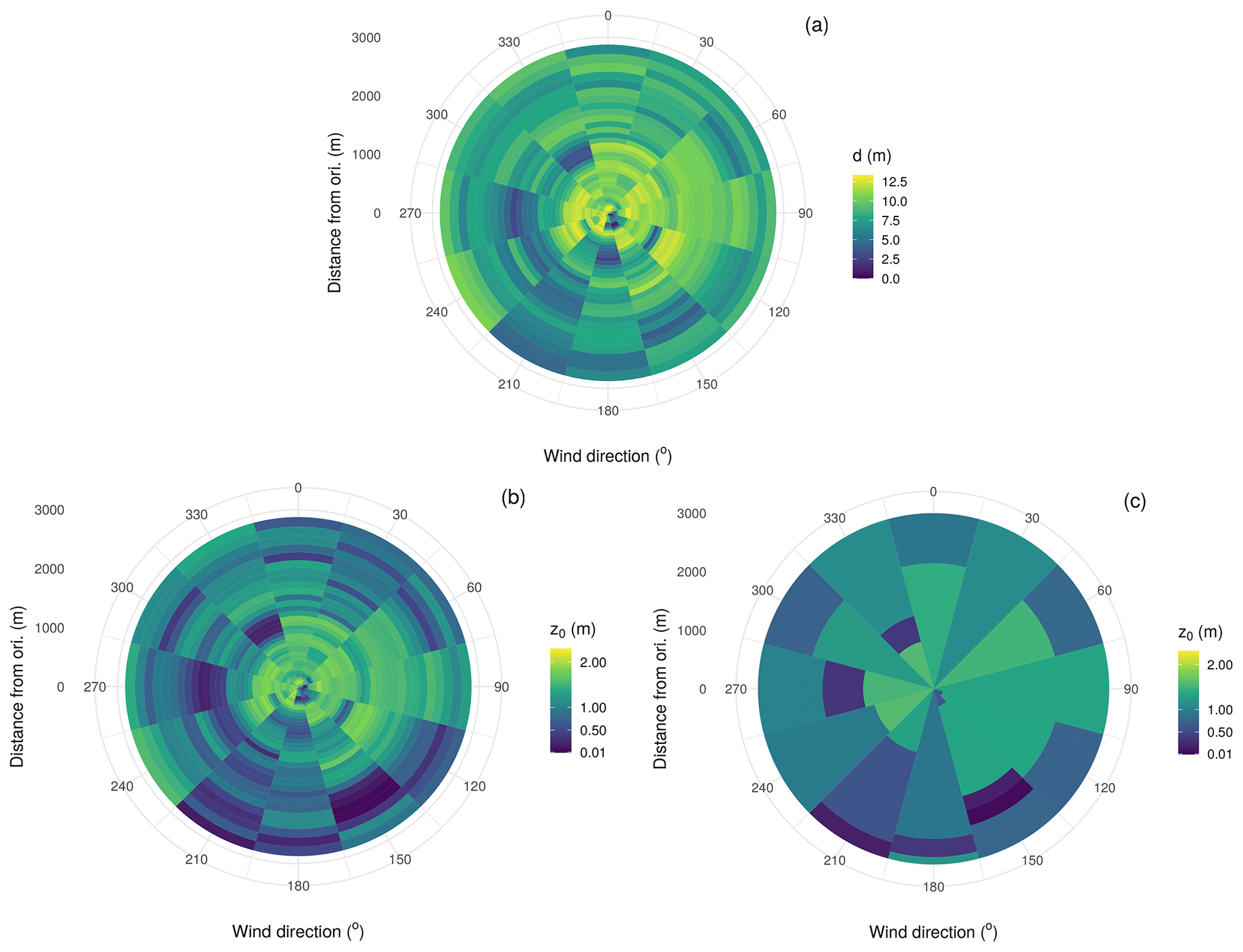
Figure 2 Example of a zooming grid analysis at the Ryningsnäs site up to 3 km distance showing the displacement height h (a), the roughness length z₀ (b), and the corresponding reduced z₀ rose (c) after finding the most significant z₀ changes.

The zooming-grid analysis of d and z₀ from the Sentinel ORA 20 map over Ryningsnäs is shown in Fig. 2a and b, respectively, as circles with a radius of 3 km. For the 0^∘ sector for an area up to 2 km away from the mast, d≈10 and z₀≈2 m, while for the 150^∘ sector at around 2 km distance there is a lake that causes lower z₀. Another detail visible from close inspection of Fig. 2a is the very low values of d and z₀ in the 150^∘ sector at distances less than 100 m away from the mast. This is because of a clearing in the forest in that direction (also seen in other sectors), which has important implications for the flow modelling at Ryningsnäs, as will be further discussed in Sect. 6. We note that Ryningsnäs was extensively investigated by Bergström et al. (2013), who fitted a logarithmic wind profile to the measurements to obtain z₀ and d. For the 150^∘ sector, d was close to zero due to the clearing, while z₀≈2 m. Their value is presumably higher than the z₀ of the clearing because it was determined at 30–40 m and therefore has a different footprint area.

Figure 2c shows a so-called reduced roughness rose, which shows the most significant z₀ changes in all directions for the same area as the zooming grid analysis. This roughness rose captures the main features of the area around the site, but it also misses some features that perhaps would have been identified using the most accurate and detailed method of manual digitalization. The large number of relatively small clearings and forest patches in all directions clearly makes it challenging to find the most significant z₀ changes.

To account for roughness changes, WAsP calculates sector-wise speedup factors for a certain point. Because the effect of a roughness change on the wind speed in a sector is distance dependent, with nearby areas having a higher impact, the distance to each z₀ area is multiplied with an exponential weighting function as described in Floors et al. (2018). From these weighted values z_0w, the ones that explain most of the variance of z_0w are stored for further processing (up to a maximum of n_max). This is done for computational efficiency, so that equations that take into account the effect of internal boundary layers can be used. These equations are given in Sect. 8.3 of Troen and Petersen (1989). The output of these equations are sector-wise speed-up factors, which are used to remove the effect that microscale features may have on the wind observations. Apart from the speed-up factors, z_0w is also used to compute a geostrophic (sometimes referred to as an effective or mesoscale) roughness length z₀G.

Similarly to z₀, d also has to be filtered to use in Eq. (1) and the geostrophic drag law. Therefore, a triangular weighting function is applied to the zooming d-grid. The average d_G in each sector is found by taking the triangular weighted average up to a distance x_d=10d₀, with d₀ defined as d at the first cell in the zooming grid at a distance x₀ from the origin. The triangular weight w is 1 at x₀ and w=0 when x>x_d. Physically the reason for applying this filter is that it takes some time for a new logarithmic profile to develop. Thus, taller trees will need a fetch to lead to an effective d_G that is applied in Eq. (1). The sector-wise z₀G and d_G can finally be used in connection with Eq. (1) and the geostrophic drag law to find a geostrophic wind climate from an input histogram. This procedure is unaltered from the description in chap. 8.7 of Troen and Petersen (1989) and is therefore not further described.

4.1.3 Orographic submodel

The submodule for orography computes speed-ups due to elevation, and WAsP uses the Bessel expansion on a zooming grid (BZ) model (Troen, 1990). The input to the orographic model is a map with elevation lines, which are processed into a polar zooming grid, with the highest radial resolution at the centre point of the grid. The resolution of the zooming grid depends on the radius R being large enough so that the entire map of height contours is contained inside the circle with radius R. Contour lines that are more than 20 km away from the site are ignored.

Here we are interested in the effects of z₀ on flow modelling, and therefore the highest-quality terrain elevation map is chosen for each of the eight sites (see Sect. 3.3). We then study the impact of varying the land cover maps only, while keeping the elevation map constant.

The resulting zooming grid of d obtained by using Eq. (11) is added to the terrain elevation zooming grid. Using this grid, the methodology described in Troen (1990) is used to calculate sector-wise wind-speed-independent orographic speed-ups. Similarly to the roughness speed-ups, these are used as local perturbations to the flow, which can be used to obtain a wind climate that is representative for a large area.

4.2 Cross-prediction analyses

We first perform cross-prediction analyses using the standard land cover databases (GLCC 1000, MODIS 500, GLOB 300, and CORINE 100) in combination with their respective un-modified translation tables leading to z₀ (Appendix A). Then, we consider the same input data sets with the modified tables from Dörenkämper et al. (2020) and Badger et al. (2015). Finally, we perform the cross-predictions using the novel Sentinel data sets, the manually digitized maps, and the lidar scans (see Table 3).

At some sites, there are multiple masts measuring at the same time (see Table 1), and the wind climate from one mast is used to predict the wind resource at the neighbouring mast. At other sites, only one mast is available and only vertical cross-predictions are possible, i.e. predictions of the wind distribution from one height to another at the same mast. We exclude observations within the roughness sublayer where the WAsP model does not apply, so only measurements between 20 and 200 m are used. In total there are 914 cross-predictions for the CORINE 100 (only Europe) database and 950 for all the other databases and Sentinel-based maps. This number is based on all possible cup anemometer pairs per site in Table 1, subtracting the combinations where a cup anemometer input is used to predict the wind climate at the exact same point (a so-called self-prediction).

Observed wind climates are generated for each height and mast from the 10 min time series of wind speed U and wind direction θ, which are discretized into histograms using a bin width of 1 m s⁻¹ and 30^∘, respectively.

The power per unit area swept by wind turbine blades, P (also referred to as the power density), is given by

$$\begin{array}{}\text{(12)}& P=\mathrm{0.5}\mathit{\rho }{U}^{\mathrm{3}},\end{array}$$

where ρ is the air density. In WAsP, the wind distribution is described by sector-wise Weibull distributions, and therefore we can conveniently find P from the Weibull parameters A and k for N_d sectors as

$$\begin{array}{}\text{(13)}& P=\mathit{\rho }\sum _{i=\mathrm{1}}^{N_d}{\mathit{\varphi }}_i{A}_i^{\mathrm{3}}\mathrm{\Gamma }\left(\mathrm{1}+\mathrm{3}/k_i\right),\end{array}$$

where ϕ is the sector frequency, Γ is the gamma function, and ρ is calculated according to the methods described in Floors and Nielsen (2019). Throughout this paper we choose to evaluate relative errors of power density,

$$\begin{array}{}\text{(14)}& {\mathit{\epsilon }}_P=\mathrm{100}\left({\displaystyle \frac{P_{\text{mod}}}{P_{\text{obs}}}}-\mathrm{1}\right),\end{array}$$

where P is obtained from the modelled (mod) or observed (obs) Weibull distributions. The statistics reported throughout the rest of the paper are the bias, $\stackrel{\mathrm{‾}}{{\mathit{\epsilon }}_P}$, and the root-mean-square error (RMSE), $\sqrt{\stackrel{\mathrm{‾}}{{\mathit{\epsilon }}_P^{\mathrm{2}}}}$, where the overbar denotes a mean. We also include relative errors in wind speed U, which we obtain as in Eq. (14) but instead of P, U is computed from the Weibull distributions as

$$\begin{array}{}\text{(15)}& U=\sum _{i=\mathrm{1}}^{N_d}{\mathit{\varphi }}_i{A}_i\mathrm{\Gamma }\left(\mathrm{1}+\mathrm{1}/k_i\right).\end{array}$$

5 Results

In the following, we show results of the three different forest models that were implemented. We present the outcome of cross-prediction analyses per site, and subsequently, we aggregate results for all eight sites investigated.

5.1 Model response to LAI

The behaviour of the three forest roughness models for a canopy height h of 10 m as a function of LAI is shown in Fig. 3. The ORA model does not depend on LAI and is therefore constant, i.e. $d/h=\mathrm{2}/\mathrm{3}$ and $z_{\mathrm{0}}/h=\mathrm{0.1}$. The Raupach and SCADIS models both show an increasing d as the LAI increases. z₀ has the opposite behaviour and decreases to lower values after an initial maximum of around LAI ≈ 1.

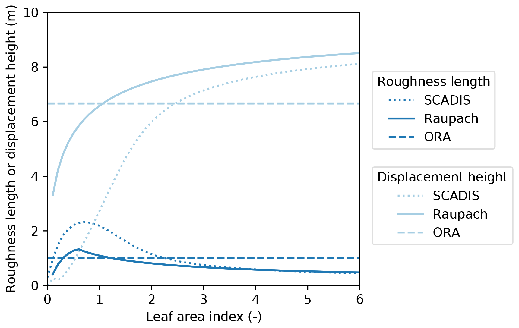
Figure 3 Response of the different roughness length and displacement height models to leaf area index (LAI) for a forest with h=10 m. The SCADIS model is set up with α=9 and β=3, which are typical values for forests with most of the canopy density in the upper part of the canopy layer (Sogachev et al., 2017).

The main differences between the SCADIS and Raupach models occur for a relatively low LAI ∼1, using the SCADIS model z₀≈2 m while using the Raupach model z₀≈1 m. The same holds for d, where using the Raupach model yields a d that is nearly twice that of the SCADIS model. For the more commonly occurring LAI >3, the differences are minor. When a different canopy profile is specified, i.e. using α=5 and β=3, there are larger differences between the two models (not shown).

5.2 Roughness length maps

Figure 4 illustrates the different z₀ representations for a 6×6 km area around the Ryningsnäs mast. The GLCC database has the coarsest resolution of 1000 m, and therefore, it fails to capture any detail near the mast (Fig. 4a). The whole area is represented by land cover class 14, i.e. evergreen needle-leaf forest, which corresponds to z₀=1.5 m (Table A1). Likewise, the MODIS database at 500 m resolution does not capture any detail within the selected area (Fig. 4b), and everything is represented as evergreen needle-leaf forest with z₀=1.0 m (Table A2). GlobCover, with a resolution of 300 m, represents most of the land cover around the site as evergreen needle-leaf forest with z₀=1.5 m (Table A1) and can capture some of the lakes and open areas (Fig. 4c). The Corine land cover database captures more details due to its higher resolution of 100 m (Fig. 4d). Most of the area around the mast is classified as “mixed forest” with z₀=1.1 m (Table A4). The lakes to the southeast of the masts and the open area to the west of the masts are captured. The Sentinel ORA 20 map (Fig. 4e) shows the result of combining the land cover map with the tree height and LAI layers according to the procedure presented in Sect. 3.2.2 and using the conversion of h to z₀ and d from ORA (Sect. 2.2.1). The Sentinel SCADIS and Raupach maps look very similar to this and are therefore not shown. It can be seen that the map generally contains a wider range of z₀, ranging from 0.0002 to over 3 m.

Figure 4 Roughness lengths obtained from a 6×6 km square around the Ryningsnäs site (red point) from standard land cover data sets (a–d), novel Sentinel data sets (e), and aerial lidar scans (f). The time periods for which the different data sets are obtained are shown in Table 2.

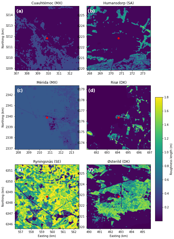
Figure 5 Roughness lengths obtained from a 6×6 km square around the meteorological mast (red point) from Cuauhtémoc (a), Humansdorp (b), Mérida (c), Risø (d), Ryningsnäs (e), and mast 1 at Østerild (f) from the Sentinel ORA 20 maps.

Finally, the z₀ map obtained using the ORA approach with h obtained from lidar scans is shown in Fig. 4f. Spatially comparing the Sentinel-based tree heights (Fig. 4e) with tree heights derived from aerial lidar scans (Fig. 4f) reveals that the areas with lower and higher h correspond very well. However, z₀ derived from Sentinel is generally lower than from the lidar scans. In Fig. 5 we show the roughness length around all the sites except the Finnish and Swedish sites, which are confidential.

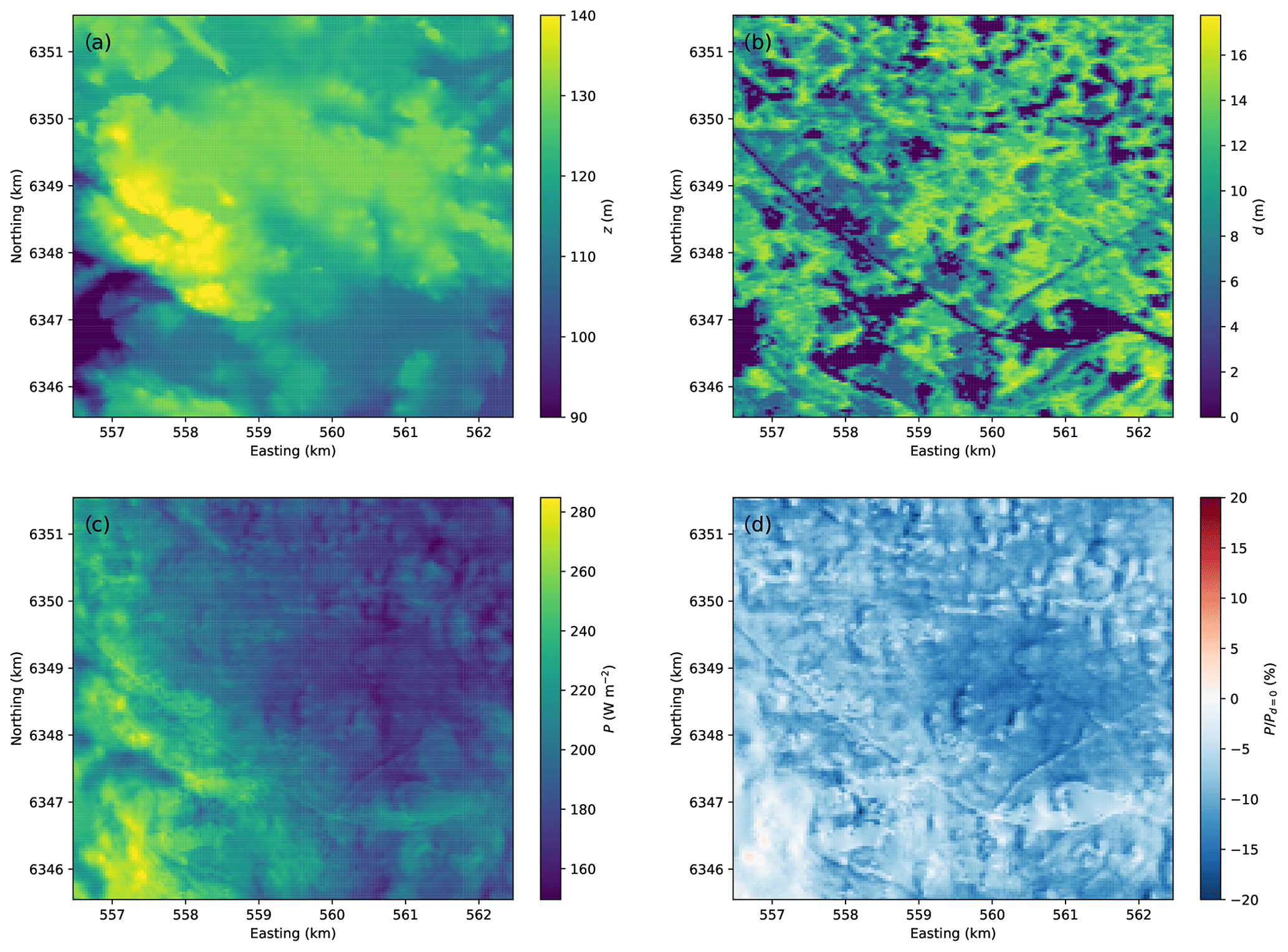
Figure 6 Maps showing the terrain elevation (a), the displacement height (b), the power density (c), and the relative difference in power density compared to a terrain map where d=0 (d) at Ryningsnäs for westerly winds.

As an example of the new routines presented in Sect. 4.1.2, we use the observed wind speed histogram at the Ryningsnäs mast at 80 m and predict the wind resource at 80 m for every point in the 6 × 6 km area shown in Fig. 4 using a raster with a resolution of 40 m. Figure 6 shows the resulting maps of the terrain elevation, displacement height, power density, and relative difference before and after d is taken into account.

The elevation changes are modest at the Ryningsnäs site (Fig. 6a), but there is a hill to the west. In Fig. 6b, the displacement height in each point is shown. For clarity, we only focus on d for the most frequently observed westerly sector. The clearing located southeast of the mast (which is in the centre of the map) is visible, resulting in lower displacement heights. In addition, displacement heights of more than 10 m are visible further from the mast. The result of combined elevation, displacement, and roughness description on the emergent power density in the area is shown in Fig. 6c. The higher power density due to the flow speed-ups over the hill in the west is clearly visible. Because the changes in power density due to the introduction of a displacement height are difficult to discern, Fig. 6d shows the difference in percent between P with and without using a displacement height. Using d causes a decrease in power density between 0 % and 12 %. The area with the highest reduction in power density in the centre indeed corresponds closely to the area with the largest concentration of high displacement heights in Fig. 6b.

5.3 Cross-predictions at wind energy sites

The rms of ε_P per site is shown in Fig. 7. We have grouped the maps from the lidar scans and those that were manually digitized into one class, because we consider all these as reference maps, i.e. the best possible we can achieve. We find rather large errors for Mérida, Ryningsnäs, and Finland. All are forested sites with mixed vegetation patterns. This indicates a need for better flow modelling at such inhomogeneous sites. Humansdorp and Cuauhtémoc, in contrast, are characterized by a relatively simple land cover, which results in a low rms of ε_P. The cross-predictions performed using the novel Sentinel maps as input mostly lead to lower rms of ε_P than those using the standard land cover databases. However, at Mérida and Østerild the rms of ε_P from the Sentinel-based maps is not lower than those from the standard land cover databases. The former is a very complex site that is characterized by forest in all directions. One possible explanation for the higher errors at this site can be a clearing in the forest that is shown to the southeast in the Sentinel maps, but which does not appear in reality. At Østerild the dominating wind direction is from the west, which is subject to many wind breaks. These are not generally detected in the Sentinel-based roughness maps but contribute significantly to a higher z₀. Therefore, the background roughness for grassland that was used in the Sentinel maps (see Table A5) might be too low at Østerild. The three forest roughness models lead to very similar results for all sites.

Figure 7 The RMSE in power density (ε_P, %) obtained when each available wind sensor is used to predict the power density at the location of other wind sensors located at the same site. Values are shown for all sites. Different colours refer to different roughness length maps used as input to the calculation.

If we consider only the cross-predictions for sites where aerial lidar scans are available (i.e. Ryningsnäs, Sweden, Finland, and Østerild), we can calculate that the combined rms of ε_P≈10.9 % for the aerial lidar scans (lidar scans ORA 20) and 10.7 % for the Sentinel ORA 20 maps, respectively. At Ryningsnäs, Finland, and Østerild the aerial lidar scans yield lower rms of ε_P than the Sentinel maps, whereas at the Swedish site results are more comparable.

When we consider the sites with manually digitized maps only (i.e. Humansdorp, Mérida, Cuauhtémoc, Risø), the rms of ε_P is 10.9 % for the manually digitized map, 13.1 % for the Sentinel ORA 20 map, and 17.3 % for the GLOB 300 map. Thus, averaged over these four sites, satellite-derived estimates of z₀ do not yield better power predictions than those based on manually digitized maps.

5.4 Aggregated results of cross-predictions

We aggregate results from the cross-predictions for the eight sites to obtain the average performance of each set of input data in connection with flow modelling in WAsP.

Table 4 RMSE in power density (ε_P, %) and wind speed (ε_U, %) for all sites combined. For GLOB 300 and CORINE 100 both the original and revised land cover databases are shown (see Sect. 3.2 and Appendix A, Tables A4 and A3).

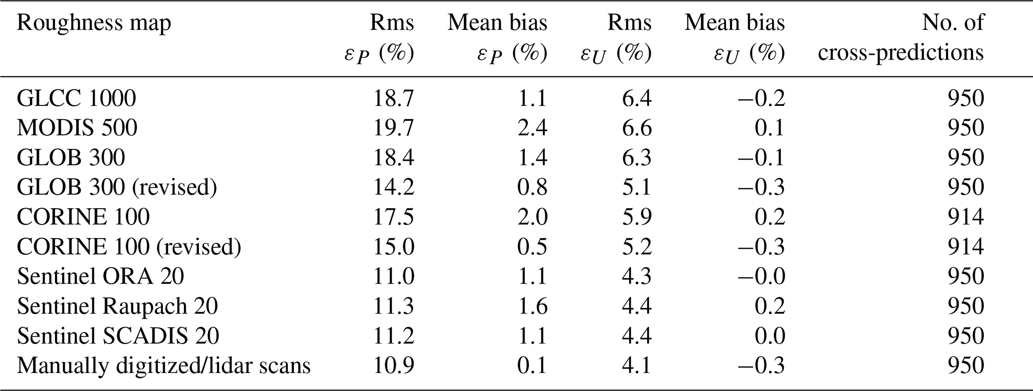
The rms of ε_P for the cross-predictions using standard land cover databases with original and revised roughness translation tables is shown in Table 4. The GLCC 1000 generally leads to the highest errors, when both the original and revised land cover tables are used. The lowest rms of ε_P of all is achieved with the GLOB 300 maps in combination with the revised land cover table. The rms of ε_P is reduced for all land cover databases when the revised land cover tables are used instead of the original ones.

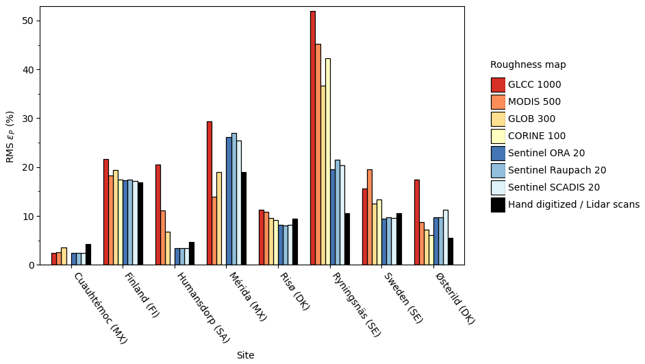
Figure 8 RMSE in power density (ε_P, %) estimated with different input maps for all eight sites combined.

We can now compare results generated with the standard land cover databases with results generated with the novel Sentinel data layers as input. Figure 8 shows the prediction errors when the WAsP model is run with seven different inputs: the three global standard land cover databases with revised roughness translation tables plus three types of Sentinel maps based on the three different forest roughness models described in Sect. 2.2. The CORINE 100 database is not available at all sites and is therefore not shown. The reference map for each site is chosen based on availability of lidar scans or a manually digitized map (see Table 3).

Maps generated with an advanced forest model (Sentinel ORA 20, Sentinel Raupach 20, and Sentinel SCADIS 20) yield lower rms of ε_P (≈11 %) than maps based on the standard land cover databases. Table 4 shows that also the mean bias of ε_P is lower in the Sentinel maps than in the standard land cover databases GLCC 1000, MODIS 500, and GLOB 300. Similarly for wind speed, the rms values of ε_U are smaller for the model runs using Sentinel maps. The mean bias in ε_U becomes slightly negative but is generally close to zero for all WAsP model runs.

When running WAsP it is often more instructive to evaluate horizontal cross-predictions, because the roughness rose will then be different for two points. To investigate this, our data were filtered to include only horizontal cross-predictions (i.e. sites with more than one mast). However, this did not change the large differences in ε_P and ε_U between the model simulations based on standard land cover databases and Sentinel maps. In addition, the effect of the measurement height was investigated by only including cross-predictions between 50 and 200 m, but again, this did not change the general picture that emerges from Table 4.

6 Discussion

For the first time, forest parameters retrieved from the Sentinel and ICESat-2 satellites have been used for wind energy flow modelling. Our results demonstrate that the spatial variability of the land cover within forests (e.g. vegetation with different height and density, clearings, lakes) is resolved far better by these novel products than it is by standard land cover products with pan-European or global coverage. The high level of spatial detail in the novel Sentinel data layers is almost comparable to products derived from aerial lidar scans. This is promising in connection with wind energy flow modelling because these data layers can be produced for any site in the world and updated frequently. The cost of retrieving the satellite-based forest data layers is far lower than the price of dedicated airborne lidar campaigns thanks to the open access to satellite data archives by Copernicus and NASA. From Fig. 7 it is clear that using the Sentinel maps of tree height rather than standard land cover maps has the highest benefit at sites where masts or turbines are surrounded by forest (Ryningsnäs, Finland, and Sweden). Taking the displacement height into account for such sites leads to significantly lower ε_P. Because there are seven masts at the Swedish site, leading to a large number of cross-predictions, this site has a large impact on the aggregated results (Table 4).

Using roughness derived from Sentinel canopy height maps had the greatest impact at the Ryningsnäs site: reducing the rms of ε_P by more than 50 % compared to using roughness derived from land cover maps (Fig. 7). This improvement of ε_P is due to the mast location very close to the forest edge in the westerly sector (i.e. winds coming from 265–285^∘). Because of the large impact of sector-wise displacement heights on the wind profile, the results are highly dependent on specifying the correct h. This indicates that for masts located very close to forest edges, sensitivity studies are recommended, and the Sentinel maps should be carefully calibrated.

The observed difference in h in the novel Sentinel product compared to the lidar scans at Ryningsnäs may partly be due to the uncertainty in sensing and retrieval methods that are required to convert satellite observations to canopy heights and partly due to temporal differences between the satellite and lidar products. The standard canopy height product from ICESat-2, which we used to train our model for forest height estimation, contains tree heights over a 17×100 m along-track transect and this is different from the spatial resolution of the lidar scans. Additionally, tree growth in temperate forests can be up to a few metres per year. Therefore, it is important to use the most updated h parameterization when modelling wind resources. Further research is needed to fully understand and improve the absolute accuracy of tree heights retrieved from satellite observations.

Likewise, the absolute accuracy of forest densities expressed through the LAI should be thoroughly quantified in future work. For example, the LAI used for our analyses was downscaled from a very coarse-resolution product, and the consequence of this downscaling is unknown. Differences between outputs of the three forest canopy models are small in this study. It is, however, possible that the SCADIS model is too advanced for the type of analysis performed here given the large uncertainty of the LAI input and the absence of canopy density profiles. More detailed studies at a higher number of sites, preferably with observed h and LAD profiles, are needed to validate the SCADIS model further.

Our analyses show only minor differences in rms of ε_P when cross-predictions are performed using Sentinel vs. aerial lidar scans to estimate d and z₀. These findings are promising in light of the lower cost and the global coverage of the satellite-based data layers. Manual assessments of the land surface roughness do not necessarily lead to better results. For most sites (three out of five) automated assessments based on the novel Sentinel data sets led to lower error values than manual assessments. In addition, automated procedures speed up the wind resource assessment process and remove the subjective judgement of a siting engineer. Using high-resolution input data for the automated retrieval of z₀ is essential. We have demonstrated how the small-scale roughness changes within forests are poorly resolved by standard land cover data sets, and as a consequence, z₀ and predictions of the wind power density come with large uncertainties even after revision of the roughness translation tables for forest classes.

Our results indicate that all methods considered in this paper underestimate the roughness length over forest (i.e. higher z₀ values lead to better predictions). This is possibly due to roughness length aggregation, i.e. finding z₀ for a larger area that correctly prescribes the momentum flux in surface-layer similarity in connection with Eq. (1). In this paper, the larger-scale sector-wise roughness length z₀G is obtained via simple logarithmic averaging of the cells in the spider-grid rose applied in Eq. (10), but this is known to be flawed in heterogeneous conditions. For example, Taylor (1987) suggested accounting for sub-grid variance of z₀ when calculating an effective roughness length. Vihma and Savijärvi (1991) compared model approaches for several landscape configurations in Finland and found that z_0eff was always higher than a simple logarithmic average. This was also confirmed by Hasager and Jensen (1999), who found that the difference between the logarithmic average and z_0eff was higher for landscapes with small patches and with a half-to-half mix of rough and smooth patches. For small patches, one can argue that the form drag of the forest will always lead to a much higher z_0eff than implied through logarithmic averaging. However, an analysis of the effect of z₀ aggregation was not attempted in this study, but its impacts are likely large for heterogeneous sites like Østerild, Finland, and Ryningsnäs. Bottema et al. (1998) reviewed a range of z₀ aggregation methods, which could be investigated in future work.

In this study, cross-prediction is used without any manual interference. For an actual wind energy project, much smaller errors would be achieved using the WAsP model because the site engineer usually has access to measurements at several heights, which can be used to fit the model nearly perfectly to the observed mean wind profile. However, such a fitting process can be deceiving, because a good fit is influenced by both z₀ and atmospheric stability conditions. It may thus me subject to compensating errors. The effect of atmospheric stability is beyond the scope of this study, and the default settings in WAsP are used, but it is acknowledged that there can be deviations at some sites.

7 Conclusions

We have tested a novel satellite-based product for land surface parameterization in forested areas and quantified the effect of using this product for wind resource modelling. The novel satellite-based product is based on observations from Sentinel-1, Sentinel-2, and ICESat-2, and it contains collocated layers of land cover, tree heights, and LAI at a 20 m spatial resolution. These maps are converted to maps of roughness lengths and displacement heights using three different forest modules of varying complexity. The simplest way to convert the tree height to z₀ and d is by multiplying with a constant (e.g. $\mathrm{1}/\mathrm{10}$). Secondly, a physically more advanced approach, which also considers the effect of LAI, is implemented. The third module is a 1D version of the SCADIS model, and it takes the effects of varying LAI and canopy density profiles into account. All three forest modules are used in the WAsP model, which is frequently used for predicting the wind resources from wind measurements.

We show that the high land cover variability of forested landscapes is poorly resolved by global and pan-European land cover databases such as GLCC, MODIS, CORINE, and GlobCover. The novel satellite-based product leads to more detailed maps of z₀ and d, which are spatially comparable to aerial lidar scans or manually digitized maps. Retrieving canopy heights from satellite data alone is a rapidly evolving branch of research – driven by the recent release of global calibration data sets such as ICESat-2 and GEDI. Further research is ongoing to refine the satellite-based products. This can be achieved through collection of larger and more accurate training data sets for the tree height retrieval, the integration of ground-based tree height observations, improved geolocation of satellite-derived products, and advancements in machine learning algorithms.

Cross-predictions are performed at eight sites with tall masts to evaluate the effect of using different input data sets in connection with flow modelling in WAsP. The novel maps from Sentinel lead to a reduction of the rms of relative errors in power density at most sites and on average by ≈3 % compared to the best performing roughness map obtained from a coarse-resolution land cover database. This is even after the roughness lengths for specific land cover categories in the coarse-resolution products are improved. Differences between the three forest modules are minor, showing that the sensitivity of the WAsP model to different approaches to obtain z₀ and d is low.

The rms of relative errors in power density found for the Sentinel ORA maps (10.7 %) is comparable to those obtained from aerial lidar scans (10.9 %). This finding is very promising because the novel satellite-based maps of z₀ and d can be generated at a lower cost and a higher temporal resolution than aerial lidar campaigns. Processing of the satellite-based maps is fully automated. For sites that show a potential for wind power projects, the new routines and products could replace current practices of land cover analysis, which is time-consuming and plagued by subjective assessments.

Appendix A

The land cover tables for the land cover databases that were investigated in this paper are supplied in Tables A1–A5. The references to the land cover databases can be found in Sect. 3.2.1.

Table A1 Land cover table used for the GLCC database (Thøgersen, 2021).

Table A2 Land cover table used for the MODIS-based maps (Thøgersen, 2021).

Table A3 Land cover table used for the GlobCover/ESA-CCI database (Thøgersen, 2021).

Table A4 Land cover table used for the CORINE database (Thøgersen, 2021).

Table A5 Land cover table used for the Sentinel-based maps.