the Creative Commons Attribution 4.0 License.
the Creative Commons Attribution 4.0 License.
 | 09 Nov 2021
Some effects of flow expansion on the aerodynamics of horizontal-axis wind turbines
David H. Wood
Eric J. Limacher
The flow upwind of an energy-extracting horizontal-axis wind turbine expands as it approaches the rotor, and the expansion continues in the vorticity-bearing wake behind the rotor. The upwind expansion has long been known to influence the axial momentum equation through the axial component of the pressure, although the extent of the influence has not been quantified. Starting with the impulse analysis of Limacher and Wood (2020), but making no further use of impulse techniques, we derive its exact expression when the rotor is a circumferentially uniform disc. This expression, which depends on the radial velocity and the axial induction factor, is added to the thrust equation containing the pressure on the back of the disc. Removing the pressure to obtain a practically useful equation shows the axial induction in the far wake is twice the value at the rotor only at high tip speed ratio and only if the relationship between vortex pitch and axial induction in non-expanding flow carries over to the expanding case. At high tip speed ratio, we assume that the expanding wake approaches the Joukowsky model of a hub vortex on the axis of rotation and tip vortices originating from each blade. The additional assumption that the helical tip vortices have constant pitch allows a semi-analytic treatment of their effect on the rotor flow. Expansion modifies the relation between the pitch and induced axial velocity so that the far-wake area and induction are significantly less than twice the values at the rotor. There is a moderate decrease – about 6 % – in the power production, and a similar size error occurs in the familiar axial momentum equation involving the axial velocity.
- Article
(1063 KB) - Full-text XML
- BibTeX
- EndNote


Conservation of axial and angular momentum are fundamental principles for wind turbine analysis. They are applied using control volumes (CVs) such as those in Fig. 1 or, more commonly, to a CV coinciding with a mean streamtube and extending into the far wake, the hypothetical region of no further wake development. For blade-element momentum theory, the CVs become expanding annular streamtubes intersecting the elements. The change in axial or angular momentum of the flow determines the net thrust or torque, respectively, acting on the rotor or blade elements (e.g. Burton et al., 2011; Hansen, 2015; Sørensen, 2016). Angular momentum is easier to analyze because in most cases it is generated only at the blades.
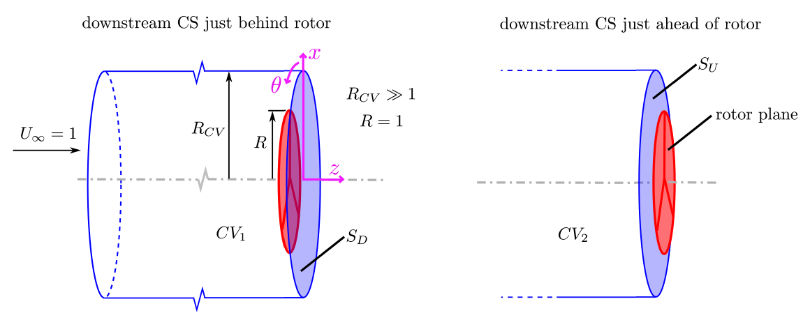
Figure 1Control volumes (CVs) to be used in the present analysis. In both variants, the upstream face extends in z to −∞, where the velocity is the wind speed, and RCV≫R. The downstream control surface is just downstream and just upstream of the rotor plane in CV1 and CV2, respectively, and the corresponding downstream control surfaces (CS) are labelled SD and SU. Taken from LW.
When a turbine extracts kinetic energy from the wind, the flow must expand both upwind and downwind of the rotor. As noted on p. 185 of Glauert (1935) and by Goorjian (1972), the axial momentum equation may receive contributions from the pressure in the expanding flow upwind of the rotor. The expansion causes the pressure force to have an axial component which alters the rotor thrust by an amount equal to the momentum flux external to the rotor. This is because the pressure forces acting on the cylindrical control surfaces at radius RCV in Fig. 1 are entirely radial. Although the role of pressure has been recognized for a long time and is discussed by Sørensen (2016) and van Kuik (2018) among others, a satisfactory analysis of it is lacking. The first main result of the present analysis is a closed-form expression for the pressure force for a circumferentially uniform rotor.
Limacher and Wood (2020) (hereinafter “LW”) investigated steady wind turbine thrust, T, using an impulse analysis, whereby the pressure in the axial momentum equation for any CV is replaced by terms that include vorticity fluxes across the CV boundaries. This removal of pressure is achieved by the substitution of various integral identities into a standard momentum-based control volume analysis, as demonstrated by Noca (1997). We will use what we call the “impulse perspective” as explained below but not impulse techniques in this paper; the interested reader is referred to LW for a short history and more details. LW showed that by approximating a rotor as an actuator disc, T is given exactly by integration over the face SD of CV1, situated just downwind of the rotor on the left of Fig. 1:
where ρ is the air density, and w is the circumferential velocity (in the direction of θ in Fig. 1) on SD; in LW, w denoted the circumferential velocity at the rotor plane, which was assumed to be one-half that on SD. This assumption is also used in the present analysis. λ is the tip speed ratio (λ>0 for clockwise rotation, as viewed from the positive z axis), and x is the radius normalized by the tip radius so that x≤1 for the rotor. The downwind face of the second CV in the figure, SU, is just upwind of the rotor. The term “exact” will be used throughout this paper to indicate that no assumptions beyond those listed below have been invoked. Taking the “wake” to be the flow that has passed through the rotor, which rotates with a constant angular velocity, these assumptions are as follows:
-
the flow upwind of the rotor and outside the wake is inviscid, steady, and spatially uniform;
-
the total energy of the wake is reduced instantaneously at the rotor, after which it is conserved;
-
viscous and/or Reynolds stresses can be neglected on the CV surfaces;
-
the axial, u, and radial velocity, v, are continuous through the rotor disc;
-
viscous drag is negligible;
-
w is zero in the upwind flow and outside the wake;
-
the vorticity in the wake is concentrated in line vortices or vortex sheets aligned with the local streamlines in the rotating frame of reference – in other words, the wake vortices rotate rigidly with the blades and vortex lines and streamlines coincide;
-
to derive the local or differential form of Eq. (1), the vorticity piercing the lateral boundaries of the annular CVs intersecting the blade elements must have no effect on the element's thrust.
Assumption no. 7 simplifies the terms involving the trailing vorticity crossing SD in the impulse derivation. Assumptions no. 3, no. 5, and no. 8 are likewise embedded in the equations derived by LW and are not explicitly required in the analysis to follow. As LW note, a thorough investigation of assumption no. 8 remains an important area of future research, but as yet the assumption remains necessary to recover the Kutta–Joukowsky expression for local thrust that is conventionally employed in blade-element momentum (BEM) analyses. As such, we perpetuate the use of assumption no. 8 for the time being. We also note, emphatically, that none of the eight assumptions places any restrictions on flow expansion. Since the impulse derivation of Eq. (1) is likewise unrestricted, the equation is exact in the presence of flow expansion and for any distribution of w(x).
Although Eq. (1) has been known since Glauert (1935) and appears in modern texts, such as Eq. (4.6) in van Kuik (2018), LW's analysis provides the first proof of its exactness when the trailing vortex sheets have finite thickness. LW's second main finding for circumferentially uniform, expanding flow is
where (when u is normalized by the wind speed, U0) is the usual axial induction factor. To maintain consistency we use only normalized velocities from here on. The easiest was to do this is to mentally replace the density ρ by .
van Kuik (2020) found Eq. (2) was satisfied by his model of the expanding flow through a wind turbine rotor. When a and v are further assumed to be C0 continuous on SU and SD, Eq. (2) tells us that at some radial location, and LW cite three simulations that show near the rotor tip. The vanishing of the first integral on SU in Eq. (2) is the more general result; the vanishing of the second integral on SD follows from assumption no. 4 above. Until the end of Sect. 3, we treat the rotor as circumferentially uniform. Since Eq. (1) contains no terms representing pressure redistribution, LW assert that its local version giving the contribution to the thrust at radius x is also exact:
where θ is the circumferential co-ordinate, defined in Fig. 1. This result is also not new: it is, for example, Eq. (4.24) of van Kuik (2018). It is often referred to as the Kutta–Joukowsky theorem for blade-element thrust because it gives the axial force, , as the product of the circumferential velocity at the rotor, , and the sum of the circulation on all blades, 2πwx. Impulse analysis, however, can also be applied if the CV outlet is moved to the far wake to give in terms of the w in the far wake. The Glauert (1935) original derivation of Eq. (1) – based on the Bernoulli equation – also suggests the exactness of Eq. (3).
Equation (2) can be derived using standard CV momentum analysis, but the authors are unaware of it appearing in the literature prior to LW. It is a natural outcome of the impulse perspective which we use to investigate the effects of flow expansion on the conventional axial momentum equation. It will be shown that Eq. (2) is closely related to the effects of pressure in the upwind flow on the conventional axial momentum equation and the general relationship between a and the far-wake induction, a∞. T is derived in Sect. 4 of Sørensen (2016) and Sect. 5.2.4 of van Kuik (2018) using a CV ending in the far wake. We take the different approach of using the CVs shown in Fig. 1 because that choice clarifies the effects of expansion. We also make further use of the impulse form of the T equation. The derivations of the remaining equations in this paper are straightforward and could have been easily done in the past if the impulse perspective had been available.
For context, we now examine the connection between the impulse- and momentum-based approaches to turbine thrust, which requires a relationship between a and w. As explained by, for example, Wood et al. (2021), the Kawada–Hardin (KH) equations for the velocity field of a constant pitch, p, constant radius helical vortex, Kawada (1936) and Hardin (1982), yield
as only half of the near-wake azimuthal velocity is induced by the wake (the other half is due to the blades). Pitch can also be related geometrically to a and λ by treating the wake as a non-expanding rigid helicoidal surface, as done by Okulov and Sørensen (2008). In the limit where λx≫w, we have
and the preceding two equations can be combined to give . The high-λ limit of Eq. (3) thus becomes
recovering the familiar 4a(1−a) integrand from classical momentum theory. At smaller λ, the relationship between the momentum- and impulse-based thrust expressions has not been fully investigated.
In the next section, we express the contribution of pressure on the expanding upstream streamtube to actuator disc thrust. The section thereafter analyzes the local form of the thrust equation. It contains our second main result about the behaviour of a – that it is negligible at λ=0 and a∞≈2a is possible at high λ only if Eq. (4) remains valid for expanding flow. In Sect. 4, we apply the Biot–Savart law to an expanding Joukowsky wake, which contains only hub and tip vortices. On the further assumption of constant p, we show, again for the first time, that depending on the extent of the vortex expansion; the larger the expansion, the closer a approaches a∞. Not surprisingly, the far-wake radius is reduced as is the power extracted by the turbine. The final two sections contain the general discussion and conclusions, respectively.
Some results of the impulse analysis can be converted easily to conventional equations containing the axial velocity and the pressure on the CV surface even when the flow expands through the rotor. For example, Bernoulli's equation for PU, the pressure on SU, is
PU and all pressures considered herein are gauge pressures relative to the free-stream pressure in the wind. Equation (7) allows the removal of v2 from Eq. (2) to give
which is also the outcome of a conventional momentum balance on CV2. The momentum balance on CV1 yields
where PD is the pressure on SD. It is important to note that the effective upper limit on the integrals in Eq. (9) is outside the rotor. Nevertheless,
since PD=PU for x>1. In other words, there is no pressure jump at z=0 outside the rotor. The thrust equation with integration only over the rotor can be found by rewriting Eq. (9) as
To remove the last two integrals for x≥1, we use Eq. (7) for PD=PU and then Eq. (2) to arrive at
The first integral in Eq. (12) contributes half of the conventional thrust. The first and second integrals are components of conventional CV analysis, whereas the third integral is new. It makes Eq. (12) exact for an actuator disc when the flow expands and will be shown below to be generally positive. We now change the CV from that shown in Fig. 1 to the more commonly used one formed by the bounding streamsurface (BS) dividing the flow passing through the rotor from the external flow. BS begins at , where z is the axial co-ordinate with origin at the rotor (Fig. 1). The vertical faces of the new CV are, therefore, subsets of those shown in Fig. 1. A straightforward momentum balance gives
where the last integrand is evaluated on BS. gives the local slope of BS, so is the axial component of the pressure acting on BS. It follows immediately from Eqs. (12) and (13) that
which gives the first quantification known to the authors of the axial force due to the expanding flow through a wind turbine rotor. It is easy to generalize this equation because there is no thrust extracted in the upwind flow. For any x and z≤0,
where S(x,z) is the streamsurface passing through (x,z) so that . The second integral is evaluated at .
PD in Eq. (12) can be evaluated in the standard manner by assuming that the unsteady Bernoulli equation is valid from immediately behind the rotor to the far wake:
where the far-wake terms have the subscript “∞”. The last two terms arise from the unsteady potential terms, evaluated by assuming rigid wake rotation (see appendix B of LW). Conveniently, these terms cancel due to conservation of angular momentum, yielding
Combining Eqs. (12) and (17) we get
where w∞ and P∞ are evaluated at x∞ in the wake, connected to x at the rotor by a mean streamsurface.
In the far wake, the pressure and circumferential velocity are related by
The relationship between the area integrals of P and w can be found using the technique introduced by McCutchen (1985) and rediscovered by Wood (2007): multiply both sides by x2 and integrate by parts for the left side. If P∞x2→0 as x↓0, and is zero at the edge of the far wake, then
As pointed out by van Kuik (2018) in conjunction with his Eq. (6.8), any swirl at the edge of the wake makes P∞(x∞)≠0. The present analysis can accommodate this behaviour, but for the present we take the simpler path of assuming P∞(x∞)=0. The main justification for this assumption is that we expect the magnitude of the swirl to become negligible everywhere at the edge of the wake at high λ. When P∞(x∞)=0, Eq. (18) reduces to
Defining the axial induction in the far wake as , we obtain
and the standard thrust equation is recovered if a∞≈2a and w2≈0, which is typically the case at high λ but may not be generally correct. Note that Eq. (22) is accurate at λ=0, where the first integral is negligible but a∞≠2a.
To recover the classical thrust equation and to provide a comparison to the analyses of Sørensen (2016) and van Kuik (2018), we now move the downwind face of the CV to the far wake and use Eq. (20). This results in
If we ignore the second integral in Eq. (18) and the integrals in Eq. (23) containing P and w, and assume a and a∞ are constant with x, we again recover the conventional relation a∞≈2a by invoking conservation of mass.
In considering the local equation for in the next section, it is useful to have the alternative form of Eq. (23) from the impulse analysis of LW. The direct application of LW's Eq. (22),
together with v=0 everywhere in the far wake and a∞=0 for r>R∞ gives
Note that Eq. (24) holds anywhere behind the rotor, i.e. for z>0 with the second integral approaching zero as .
The results for the far wake can be used to estimate the conventional thrust when λ=0, and the expansion is negligible by application to SD. Equation (20) will then be approximately valid for a and PD replacing a∞ and P∞, and comparison with Eq. (1) shows that the momentum flux term 2a(1−a) will be negligible. In other words, the thrust on a stationary disc occurs predominately through the pressure on its back face associated with w.
Having considered the thrust for the complete rotor, we now consider the local contribution at radius x. We continue to use a circumferentially uniform disc. It is easy to show that the local form of Eq. (12),
is exact for a circumferentially uniform disc in expanding flow. This can be done in at least two ways. First, using Eq. (7) and simple manipulation, the bracketed terms can be written as
and the pressure difference across the annulus containing the blade elements must give the exact thrust by assumption no. 4. Secondly, starting from Eq. (15) it is easy to prove that a2−v2 in Eq. (26) accounts for the difference in pressure acting on the top and bottom of the expanding annular streamtube that intersects the blade elements.
We now consider the consequences of the exact Eq. (26) for the far wake. If the w and P∞ terms in Eq. (17) are negligible at high λ, the bracketed term in Eq. (26) becomes
The exactness of the local form of Eq. (23) is not easy to establish in general because all three velocity components can be important in the wake and the total pressure is not constant. This is the first reason we based our analysis on the CVs shown in Fig. 1 rather than one extending to the far wake. We note, however, that there is no interchange between pressure on BS and axial momentum in the flow outside the far wake where . In other words, the interchange is completed before the far wake is reached. This is the second reason we used the CVs in Fig. 1. The local form of Eq. (23) will have a term corresponding to the bracketed term in Eq. (26) of 2u(1−u∞). Combining with Eq. (28), we retrieve the standard result that or a∞=2a which can be accurate only at high λ; note that the discussion immediately below Eq. (22) shows the result does not hold at λ=0. Further, from Eq. (7),
If Eq. (6) is valid, then Eq. (26) becomes
for x≤1.
The preceding analysis shows that in general, in contrast to the familiar results of one-dimensional momentum theory. would require a=v, which cannot hold everywhere for several reasons. First, v→0 as x↓0, whereas there is no similar constraint on a. Secondly, we argued above that the flow outside the wake has an axial momentum deficit so a≥0 but not necessarily equal to v for x>1. Equation (2) would then be violated if a=v for x≤1. Thirdly, van Kuik (2018) Sect. 5.4.4 points out that there is no theoretical requirement that . They are unlikely, however, to differ greatly in general. This suggests v→a as x→1, as argued by LW and shown by the model calculations of van Kuik (2020), who found also that v was significantly larger than a outside the wake until at least x≈1.2. If a>v over most of the rotor, then the positive a2−v2 in Eq. (26) corresponds to a positive pressure exerted by the external flow on the wake.
A more definite statement about PU and PD can be made for stationary rotors (λ=0) following the last paragraph of the previous section. It is shown there that a is negligible at λ=0 so that PU≈0 and PD is associated with w behind the rotor. The inequality reduces as λ increases but is always present because of non-zero a2−v2.
We now consider the far wake in more detail to determine the vortex pitch and its relation to a∞, which are required in the next section. Equation (19) requires when . We assume that at sufficiently high λ, the wake approximates a Joukowsky wake with the hub vortex lying along the axis of rotation and the tip vortices at radius R∞ in the far wake, with no vorticity in between. The main justification for this assumption comes from Eq. (1). When λ=0, the first term implies that the bound vorticity, Γ, cannot be constant; Wood (2015) showed that Γ∼x2. At high λ, however, the first term becomes negligible in comparison to the second for most x. The simplest wake for which the thrust remains bounded on a turbine with N blades occurs when NΓλ∼λwx is constant in x and λ; this is the Joukowsky wake in which assumption no. 7 of Sect. 1 becomes irrelevant to the flow between the tip and hub vortices. Further, the tip vortices now separate the wake and the external flow, which may have very different velocities. The vortex velocity should then be the average of these two, and the vortex lines need not align with the wake streamlines.
Outside the hub vortex core of a Joukowsky wake, and, as pointed out by Sørensen (2016), the total pressure is constant for all streamsurfaces. In addition, independence will hold in the sense that the integrands in Eqs. (23) and (25) must be equal. Thus,
without making any assumption about the relationship between a and a∞. p∞, the constant pitch of the constant radius tip vortices, is related to the velocities by the equivalent of Eq. (4): . Equation (31) can be rewritten as
In the next section, λ will be calculated using Eq. (32) for a given p∞ and the corresponding calculated value of a∞. Equation (32) is the high−λ equivalent of Eq. (22) of Okulov and Sørensen (2008) for vortex pitch provided the convection velocity of the vortex – w in their notation but wv here – is equal to . Table 1 of Wood and Okulov (2017) shows that wv→a for ideal Betz–Goldstein rotors as λ→∞, and so Eq. (32) is recovered since a∞→2a in the same limit. Another way to view this result is that the axial velocity in the Joukowsky far wake is constant and equal to 1−a∞ outside the vortex cores, so the tip vortices must travel downwind at a velocity of to be force-free.
The KH equations for a doubly infinite helical vortex of constant radius and pitch lead to
If we ignore wake expansion, then for the singly infinite near-wake, and if p∞≈p, then a∞≈2a. This result suggests the strategy for the next Section, where we analyze the flow associated with expanding tip vortices by assuming they have constant pitch everywhere. This allows a semi-analytic determination of their influence on the flow through the rotor. In other words, we relax one of the limitations of the KH equations, that of constant radius, which must be relaxed, but keep the limitation on p, which, hopefully, leads to results of sufficient generality.
We assume p remains constant and use the results of the previous section and the Biot–Savart law to investigate the flow immediately behind the rotor to determine the thrust and power coefficients. The circumferentially averaged velocities are due entirely to the trailing vorticity: w is due to the hub vortex only, whereas u and v result from the expanding tip vortices only.
4.1 Biot–Savart analysis of expanding tip vortices
Without loss of generality, let the lifting line representing one blade lie instantaneously along the x axis in Fig. 1 and consider the tip vortex beginning at (1, 0, 0). We now determine the velocities induced at a point in cylindrical polar co-ordinates or in Cartesian co-ordinates for constant p. A point on the vortex is in Cartesian co-ordinates or in cylindrical polar co-ordinates, where radius t is a monotonically increasing function of the vortex angle β that asymptotes to the far-wake radius. Thus, , and from here on, the dependence of t on β will be understood. An increment dl along the vortex is given by
and the distance d from the point to the vortex is
so that
which is an even function of β and θ. A straightforward application of the Biot–Savart law yields the three velocities associated with the trailing tip vortex as
where Γ is the vortex strength,
In forming the circumferential averages by integrating over , all the sin (β−θ) terms will vanish as they are odd in θ. The linearity of inviscid flow leads to equal contributions to the averaged from the N identical and equi-spaced trailing vortices.
The simplest calculation of ia is for x=0, for which the circumferential average , and
Ia is, clearly, dependent only on the geometry of the tip vortices. For an expanding wake with constant p, Eq. (4) will underestimate a as when t is not constant. If p varied with β, then pβ in Eq. (36) would be replaced by ∫pdβ and the direct relation between and would be lost. It is likely that an analytic expression for the integrands in Eq. (37) would not be possible.
Performing the θ integration of Eq. (40) using Mathematica gives
where . E(.) and K(.) are the complete elliptic integrals of the second and first kind, respectively, whose argument . Thus, v and a can be obtained by integrating Eq. (41) along the trajectory of the tip vortex, t(β) for . This must, in general, be done numerically, but several checks are possible. In describing these, we continue to use the notation and identify the limits to the integral if they differ from (0,∞).
If t remains constant at 1, say, and the integration is over , that is, for a doubly infinite vortex or vortices of constant radius and pitch, then for any x, and
The interior and exterior solutions in Eq. (44) are consequences of the KH equations, derived from the velocity potential. All results in Eq. (44) follow from Eq. (37). Using NIntegrate in Mathematica and MATLAB's integral, these results were reproduced to six significant figures for a similar range of x to that used in the main text and limits of ±1000π on the integration. For a singly infinite helix, the values of Ia for z=0 when β=0 are half those in Eq. (44). These were reproduced numerically to the same accuracy. Iv is not available from the KH equations for this case.
As with any Biot–Savart analysis, the behaviour of Eqs. (42) and (43) as must be considered. As mp→1, E(mp)∼1, Eq. (19.6.1) of NIST DLMF (2021), and , where , Eq. (17.3.26) of Abramowitz and Stegun (1964). The leading terms in Eqs. (42) and (43) become
showing that a logarithmic singularity occurs in ia despite it being the integrand for the circumferentially averaged axial velocity. This is a stronger singularity than that in Chattot (2020) perturbation analysis of the flow near the edge of the rotor, which assumes a vortex cylinder wake. There is no logarithmic singularity in iv, but the slope increases without bound as β→0. These behaviours could be mitigated by using the well-known cut-off modification to the limits of the Biot–Savart integrals as was done for helical vortices by Ricca (1994); see also Sect. 11.2 of Saffman (1992). There is, however, a simpler, heuristic alternative. The upper limit on a(x) as x→1 is taken to be a∞. A partial justification for this tactic comes from the wind tunnel measurements of a model wind turbine by Krogstad and Adaramola (2012). Their Fig. 9c shows that at λ=9.51, a≈0 at small x but rises to the extraordinary value of around 0.8 at x=1. Thus, was enforced in the calculations described in the main text. Whenever this was done, Iv was assumed equal to the maximum value below the limit on Ia.
The numerical evaluation of Ia and Iv can be improved by considering the asymptotic behaviour of ia and iv for large β, which corresponds to small m and mp. The leading terms are simple functions of β, allowing the infinite integrals to be approximated. For Iv, we have
where the first term was obtained numerically over and the remainder, , is an approximation to the integral over . is
The remainder for Ia is independent of x:
This result also follows from Eq. (41) when z≫R∞.
It was found that was sufficient to ensure six-figure accuracy of the integrals over the range of x considered below. Iv converged faster than Ia, reaching 99 % of the final value by β=2π for any x.
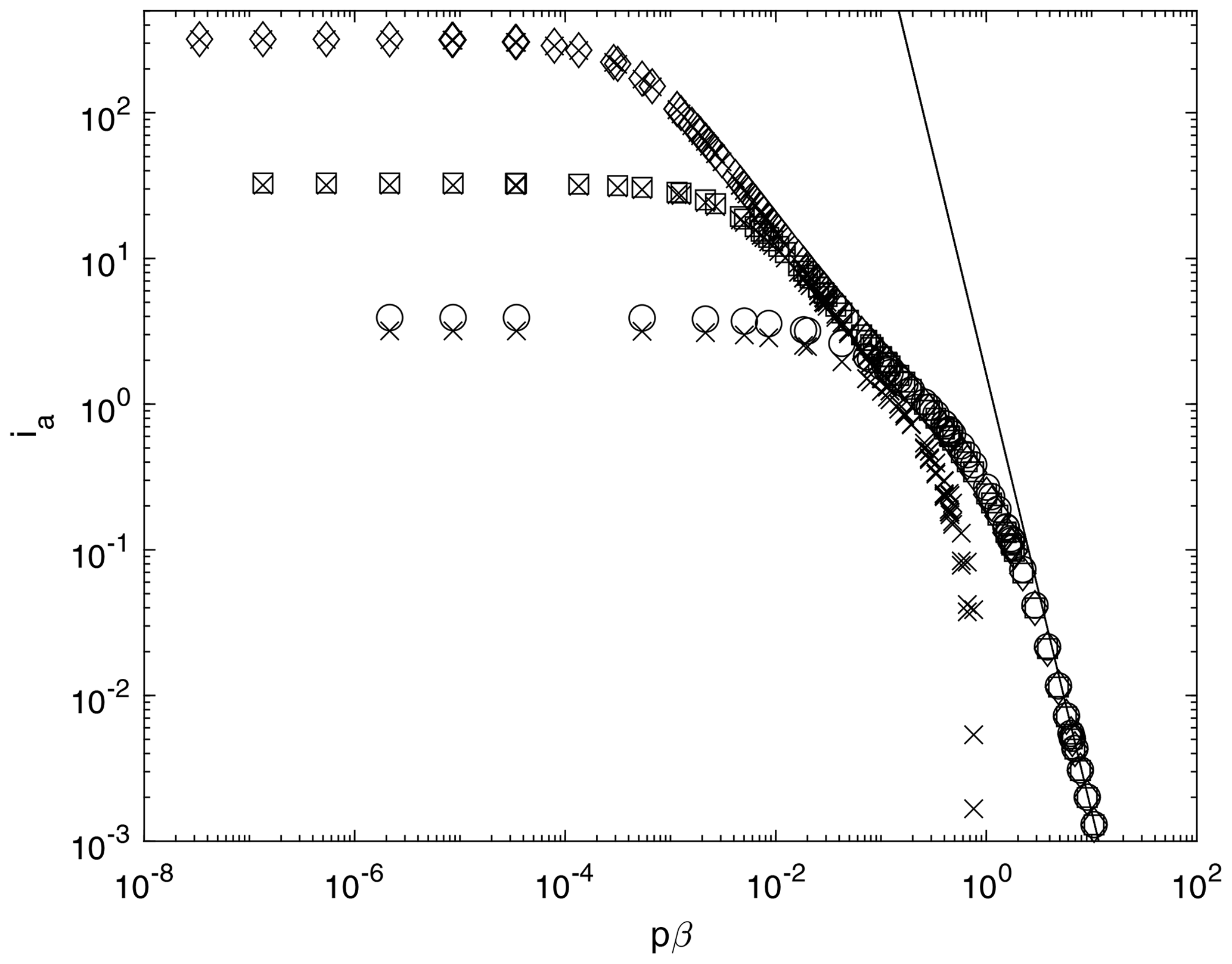
The Biot–Savart integrands in Eq. (43) are plotted in Figs. 2 and 3 for x close to the blade tip, in terms of axial distance z=pβ, where β is the vortex angle starting from zero at the rotor. The figures also show the small-β asymptotes in Eqs. (45) and (46) and the large-β remainders defined in Eqs. (48) and (49). If the tip vortex radius t remains at 1, Eq. (44) gives for any x, and the conventional momentum equation (Eq. 6) remains valid. We assume that is the minimum value of Ia, and, as explained in the Appendix, we impose a≤a∞ so that . For maximum power, the familiar derivation of the Betz–Joukowsky limit suggests , so we investigate R∞ around that value. Note, however, the use of Eq. (6) to derive this limit means that it is applicable only to a wake that expands either very slowly, as explained above, or very rapidly to , as for any constant t. We will show that generic wind turbine wakes at high λ expand at a rate that is intermediate between these extremes, which causes Eq. (6) to be inaccurate. There is no direct maximization of power output in the following analysis. Instead, the wake model is constrained as we now describe.
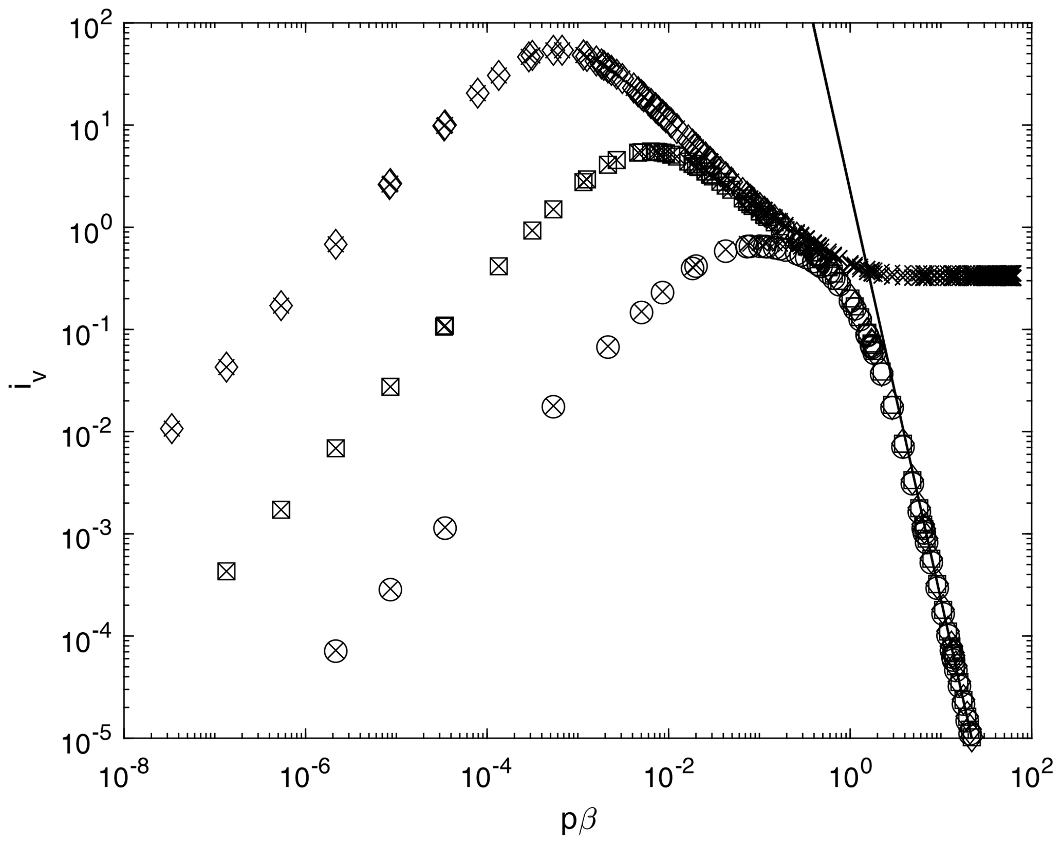
Figure 2Integrand, iv, for p=0.1, . ◦, x=0.9; □, ; and ⋄, x=0.999 from Eq. (42). iv increases with x. × is the integrand in Eq. (45). For clarity, only every second data point is plotted. The solid line shows the remainders from Eq. (48). The differences with varying x are within the thickness of the line.
Solving Eq. (37) for Ia and Iv requires p and the tip vortex trajectory. We used the very simple form:
which satisfies three necessary conditions: t=1 when β=0, t→R∞ for large β, and t and its derivatives are continuous. The fourth condition is that k must satisfy the reduced version of Eq. (2):
This integral will be called the “expansion integral”. It uniquely fixes k for any choice of and p. Ia and Iv were obtained using the MATLAB function integral over to an absolute tolerance of 10−6. The remainders, Eqs. (48) and (49), were then added. The expansion integral and the mass flux integral described below were found by trapezoidal integration using the points shown in Fig. 4. The expansion integral is large for small k as v is (not obviously) maximized when there is very little vortex expansion near the rotor.
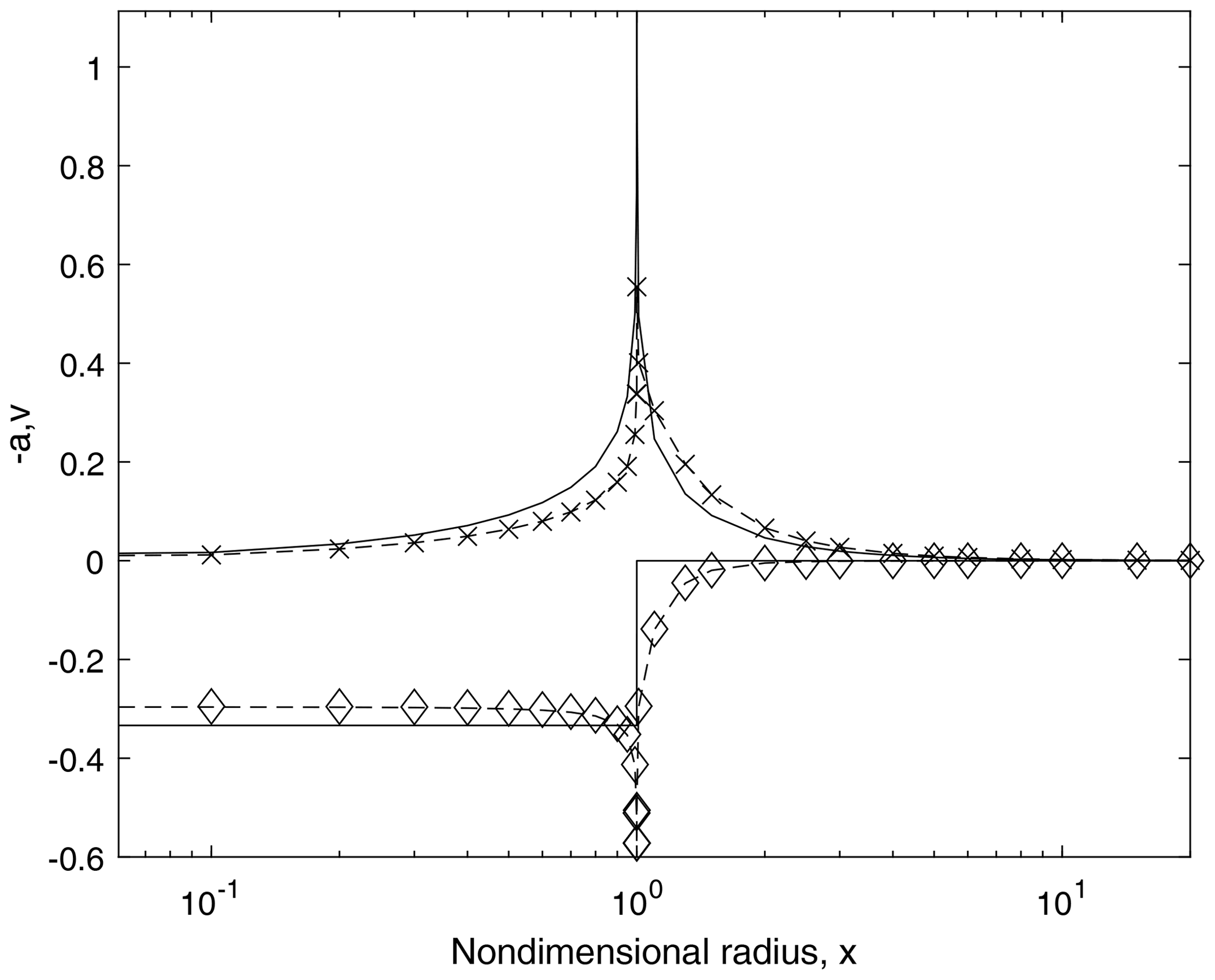
Figure 4Axial induction, a, and radial velocity, v, for the conditions in Table 1. p=0.05: a, ⋄; v, ×. The corresponding results for p=0.10 are the dashed lines. Note that −a is shown to make it distinct from v. The solid lines are −a and v for no expansion, i.e. k=0, R∞=2. The x axis is logarithmic.
The mass flux through the rotor, using Eq. (33) to remove NΓ, determines a∞:
Equation (32) then yields λ. A number of possible methods were considered for solving the integral in Eq. (52). ia(x,θ) can be written as
which allows an analytic integration of ia(x,θ)x in x. The resulting expression is complicated and probably requires numerical integration in θ and β to obtain the mass flux. Further, the integrand is singular at a point that varies with θ and β. The simpler alternative of numerical integration of Iax was used.
To find the unique , we impose the further condition that k must match the slope of the vortex surface at the rotor. Then k in Eq. (50) equals k*, given by
4.2 Results
The results in Table 1 were obtained using the MATLAB routine patternsearch to minimize the single objective function that combined the magnitude of the expansion integral and . This, surprisingly, occurred at a constant value of , implying that the vortex expansion to the far-wake radius happens over a fixed distance and the surface containing the vortices has the same shape, independent of p or λ.
Table 1Results for the expanding Joukowsky wake with constant pitch.

CT was calculated from Eq. (1) with w2 ignored because λ is large:
using Eqs. (32) and (33). We note that Eq. (1) makes the high-λ blade-element thrust constant across the rotor, whereas the familiar form involving the axial velocity equation in Eq. (6) requires a significant variation near the tip. From conservation of angular momentum, and finding the power as the product of torque and angular velocity,
so the power extraction also decreases significantly near the tip. Equation (56) and the third component of Eq. (55) also hold for the conventional analysis that leads to the Betz–Joukowsky limit.
From Table 1, the biggest change from the familiar Betz–Joukowsky wake is the 20 % reduction in , which occurs because for much of the rotor (Fig. 4). In other words, more of the expansion occurs upwind of the rotor. In contrast, the maximum CP is reduced by only 6 % to 0.557 and the mass flux is increased by 2 %. The second to last column in Table 1 gives , the conventional thrust coefficient evaluated from Eq. (6):
The positive values of in Table 1 indicate the conventional equation overestimates the thrust by around 5 %. From Eqs. (29) and (30), we get the integrated asymmetry of the disc pressure distribution at high λ as
Using the data in Table 1, the integral of δP is 0.087, so the magnitude of PD is generally significantly less than that of PU. It was shown in the previous section that the pressure integrals are equal in magnitude in the minimally expanding wake when λ=0, but the analysis in this section shows divergence in the expanding Joukowsky wake at high λ.
The integrands iv and ia Figs. 2 and 3 are large in the vicinity of the rotor. Their size implies that the simple assumed shape of the tip vortex trajectory, Eq. (50), is reasonable and that adding a term or terms, say, to control the approach to the far wake would not change the analysis significantly. The low- and high-β asymptotic approximations to iv and ia are accurate at sufficiently large x for an appropriate range of β but are not sufficiently general to yield analytic approximations to the integrals. The final figure, Fig. 5, plots the ratio of a and a∞. The large differences from a∞=2a occur near the edge of the rotor.
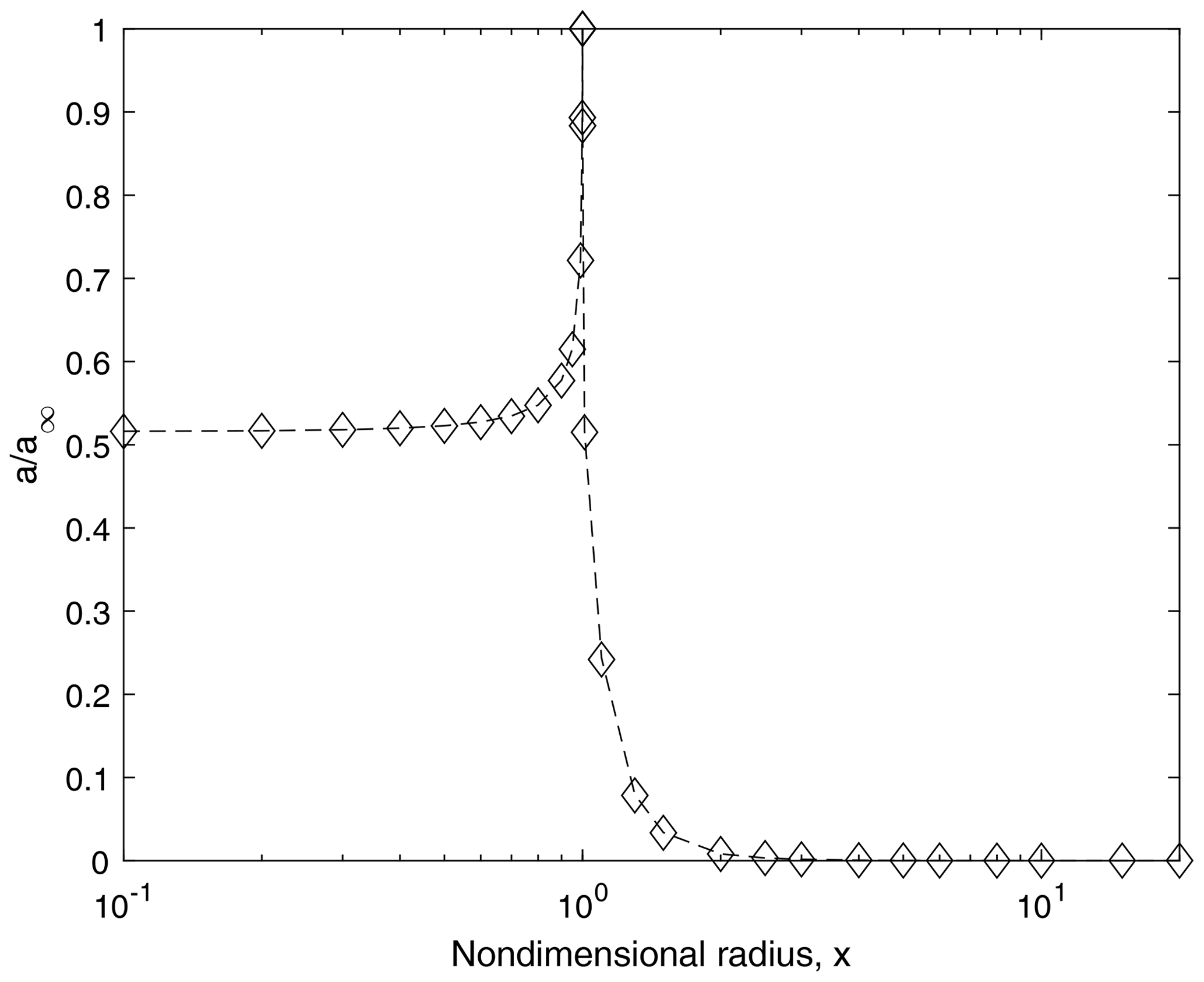
Figure 5Ratio of axial induction at the rotor, a, to value in the far wake, a∞. p=0.05; ⋄. p=0.10; dashed line. Note that the x axis is logarithmic.
Figure 4 shows that a and v at the rotor for the cases in Table 1 are independent of p. a(0)=0.296, which is less than the Betz–Joukowsky value of , and v(0)=0 as it must. The results for v and in an unexpanding wake () are plotted as solid lines. Note that a=0 for x>1, but v is very large near the edge of the rotor, and it is clear that the expansion integral cannot be satisfied. The limit a≤a∞ was applied near the blade tip for the expanding wake, where v has increased to be nearly equal but smaller than a. Outside the wake, v>a and takes until x=3 to fall to 0.03. Similarly shaped distributions of a and v for a Joukowsky wake are shown in Fig. 5 of van Kuik (2020), who also found that Eq. (2) was satisfied in his low-λ simulations.
In the final figure, Fig. 5, the ratio documents the departure from the conventional relationship a∞=2a near the rotor edge. Note that a∞ is constant for a Joukowsky wake, so the ratio is non-zero for x>1.
The pressure in the expanding flow ahead of a wind turbine contributes to the axial force on the rotor and a momentum deficit in the flow outside the rotor. Researchers have been aware of these two effects for many years, but the present analysis provides the first quantitative determination of them in Eqs. (14) and (15) derived by approximating the rotor as an actuator disc. The effects on the disc in integral and incremental form depend on a2−v2, where v is the normalized radial velocity and a is the usual axial induction factor. Further, v2−a2 can be used to quantify the external flow disturbed by the wind turbine and so may be useful to the study of multiple rotors in close proximity, as analyzed by, for example, Branlard and Meyer Forsting (2020). One way to do this is by defining IE as
where xBS is the radius of BS at any z≤0. The last integral is a consequence of Eq. (2) being valid for SU lying anywhere in the upwind flow. IE must be zero in the undisturbed upwind flow. It then increases to its maximum value at the rotor according to the present analysis. IE then decreases in the wake to be zero in the far wake. In other words, the perturbation to the external flow is complete by the time the far wake is reached. Note that the second equality in Eq. (59) does not hold in the wake.
The impulse analysis of Limacher and Wood (2020) (LW) showed that the Kutta–Joukowsky (KJ) equations for rotor thrust, Eq. (1), and for the blade-element contributions to the thrust, Eq. (3), are exact in the presence of wake expansion, where “exact” means using no more assumptions or approximations than the eight listed in the Introduction. The KJ equations, containing only the circumferential velocity and tip speed ratio, are not equivalent to the conventional equation involving only the axial velocity, when the flow expands. This is the outcome of the analysis in Sect. 4, where an expanding Joukowsky wake comprising tip and hub vortices of constant pitch was analyzed. The conventional thrust equation is altered by around 5 %–10 %, depending on the trajectory of the tip vortices because the geometrical relation in Eq. (4) is modified by the expansion.
The first three sections of the paper used only the standard form of control volume (CV) analysis for axial momentum to determine the thrust of the rotor and the incremental thrust of the blade elements comprising the rotor. To clarify the effects of expansion, most analysis in this paper used CVs with downwind faces in the immediate vicinity of the rotor, as opposed to their common placement in the far wake. The rotor and the flow are assumed to be circumferentially uniform. We argued in the Introduction that the impulse analysis provides a simple and novel perspective on the role of the pressure. The thrust equations derived in Sect. 3 for the rotor, and in Sect. 4 for the local flow at any radius, contain the pressure acting on the downwind face of the actuator disc, which must be removed to make the equations suitable for actual blade analysis. Removal can be done accurately only for very low tip speed ratios where the expansion and its effects are small.
To the rotor thrust, the pressure along the bounding streamsurface adds a term containing the integral of a2−v2 over the rotor. This integral is equal and opposite the integral for the flow outside the wake, so there is no net contribution to the thrust determined using the CVs shown in Fig. 1. Unsurprisingly, the corresponding term in the local thrust equation at any x also contains a2−v2. It follows that the conventional local thrust equation implies a≈v, but a2 is generally larger than v2 over the rotor, but more precise estimates of v do not appear to be possible. a2>v2 implies that the pressure adds to the rotor thrust and is associated with a momentum deficit in the external flow. The common derivation of the axial momentum equation, which leads to the Betz–Joukowsky limit, ignores the interaction of pressure and external momentum and then ignores the radial velocity in relating the pressure at the rear of the disc to the far wake. These errors cancel, so the main failing of the conventional equation is the breakdown of the relation a∞=2a when expansion is significant. The previous section suggests this breakdown is due to the expanding tip vortices at high λ in the Joukowsky wake. At the rotor, the slope of the streamsurface containing the tip vortices is 53∘ for maximum power extraction, Table 1, so their trajectory is intermediate between very slow and very rapid expansion, either of which would require a∞=2a. This analysis used Eq. (32) for the pitch of the tip vortex, found by moving the CV outlet to the far wake and using LW's impulse equation for thrust. We note that van Kuik (2020) estimated the streamsurface angle at the rotor edge to be 46∘, which is close to the present value. The effect of the expansion on a was constrained so that a≤a∞ as an alternative to using a cut-off in the Biot–Savart integral. Figure 4 shows that a increased with radius to reach a∞ in the streamtube bounded by the tip vortex, suggesting a very substantial effect of expansion. Qualitatively, this large value of a is in agreement with the wind tunnel measurements of Krogstad and Adaramola (2012), who found that a increased across the rotor to reach 0.8 at the tip at high λ.
Including v in the axial momentum equation effectively adds an extra unknown to the conservation equations that may render them useless unless another equation for u, v, or w could be derived. Further, high v may cause significant alterations to the lift and drag of the blade elements near the tip. To our knowledge, radial velocity effects on airfoil lift and drag have not been studied in the context of blade-element theory.
The role of the radial velocity and flow expansion is probably more complicated in rotors with a limited number of blades than the actuator discs considered here. Eriksen and Krogstad (2017) measured u, v, and w immediately behind the rotor of a model three-bladed turbine out to a radius 20 % larger than the blade tip radius. They used phase-locked averaging to obtain the flow field as seen by an observer rotating with the blades. Significant phase variations occurred in a and v, showing that the averages a2 and v2 over a blade revolution could be large even if the mean values of a and v are small. Nevertheless, the magnitude of both a and v was largest near the angular location of the blades, suggesting that the issues with radial deflection will occur in real turbines. We hope that these comments, and the present analysis, will inspire further measurements to be made far enough outside the wake to help clarify the role of flow expansion and the disturbances to the external flow.
This analysis started from the impulse-derived Kutta–Joukowsky equation for wind turbine thrust, which does not involve the axial velocity. The equation is valid for any amount of expansion in the upwind flow and the wake and any distribution of bound circulation on the rotor. We were able to
-
demonstrate the conventional thrust equation containing the axial velocity can be correct only when the tip speed ratio is large;
-
derive an exact expression for the effects of flow expansion on the conventional momentum equation – this involves the axial induction factor and the radial velocity;
-
apply the conventional and impulse thrust equations in the far wake to give the pitch of the tip vortices in the Joukowsky wake in terms of the tip speed ratio and the far-wake induction;
-
find a semi-analytic solution of the Biot–Savart law for the induced velocities at the rotor by assuming the tip vortex had constant pitch – the axial velocity near the rotor tip approached the far-wake value, but was prevented from exceeding it as an alternative to using the familiar cut-off in the Biot–Savart integrals, and the increase in the rotor value contradicts the familiar relation that the axial induction factor everywhere at the rotor is half that of the far wake; and
-
derive in Sect. 5 the following results from the model of constant pitch, expanding tip vortices:
-
the angle of the tip vortex surface to the wind direction was 53∘ for maximum power production, independently of the tip speed ratio and vortex pitch;
-
because it is neither very small nor very large, this expansion leads to an error of around 6 % in the conventional thrust equation, which would be accurate for both extreme expansions;
-
the resulting wake expands less than the familiar Betz–Joukowsky wake – for two pitch values corresponding to tip speed ratios of 7 and 14, the far-wake area was 1.59 times the rotor area;
-
we find the reduction in the rotor power and thrust due to expansion – the maximum power coefficient and corresponding thrust coefficient were 6 % less than the values given by the Betz–Joukowsky limit; and
-
we quantify the influence of the expansion on the flow outside the rotor – for example, the radial velocity at three rotor radii is still 3 % of the wind speed when the rotor is producing maximum power, and the axial induction factor decays to zero more rapidly than the radial velocity as radius.
-
All the MATLAB codes and data used in this analysis are available from the first author.
This study was conceived by both authors, who shared the analytic development. DHW completed the numerical analysis and the first draft of the manuscript, with both authors contributing equally to its revision thereafter.
The contact author has declared that neither they nor their co-authors have any competing interests.
Publisher's note: Copernicus Publications remains neutral with regard to jurisdictional claims in published maps and institutional affiliations.
This paper was inspired partly by an anonymous referee of LW who doubted the value of Eqs. (1) and (3) because they do not contain the axial velocity. We acknowledge the useful comments of Gijs van Kuik on an earlier draft of this paper. David H. Wood's contribution to this work is part of a research project on wind turbine aerodynamics funded by the NSERC Discovery Program. Eric J. Limacher acknowledges receipt of an NSERC Postdoctoral Scholarship.
This research was funded by a Canadian Natural Sciences and Engineering Research Council Discovery Grant.
This paper was edited by Jens Nørkær Sørensen and reviewed by Gijs van Kuik and Emmanuel Branlard.
Abramowitz, M. and Stegun, I. A. (Eds.): Handbook of mathematical functions with formulas, graphs, and mathematical tables (Vol. 55), US Government printing office, Washington, DC, 1964. a
Branlard, E. and Meyer Forsting, A. R.: Assessing the blockage effect of wind turbines and wind farms using an analytical vortex model, Wind Energy, 23, 2068–2086, 2020. a
Burton, T., Jenkins, N., Sharpe, D., Bossanyi, E., and Graham, M.: Wind Energy Handbook, 3rd Edn., John Wiley & Sons, Chicester, UK, 2011. a
Chattot, J. J.: On the Edge Singularity of the Actuator Disk Model, J. Solar Energ. Eng., 143, 014502-1–014502-5, 2020. a
Eriksen, P. E. and Krogstad, P. Å.: An experimental study of the wake of a model wind turbine using phase-averaging, Int. J. Heat Fluid Flow, 67, 52–62, 2017. a
Glauert, H.: Airplane propellers. In Aerodynamic theory, Springer, Berlin, Heidelberg, 169–360, 1935. a, b, c
Goorjian, P. M.: An invalid equation in the general momentum theory of the actuator disc, AIAA J., 10, 543–544, 1972. a
Hansen, M. O.: Aerodynamics of Wind Turbines, Routledge, London, New York, 2015. a
Hardin, J. C.: The velocity field induced by a helical vortex filament, Phys. Fluids, 25, 1949–1952, 1982. a
Kawada, S.: Induced velocity by helical vortices, J. Aeronaut. Sci., 36, 86–87, 1936. a
Krogstad, P. Å. and Adaramola, M. S.: Performance and near wake measurements of a model horizontal axis wind turbine, Wind Energy, 15, 743–756, 2012. a, b
Limacher, E. J. and Wood, D. H.: An impulse-based derivation of the Kutta–Joukowsky equation for wind turbine thrust, Wind Energ. Sci., 6, 191–201, https://doi.org/10.5194/wes-6-191-2021, 2021. a, b, c
McCutchen, C. W.: A theorem on swirl loss in propeller wakes, J. Aircraft, 22, 344–346, 1985. a
NIST DLMF – Digital Library of Mathematical Functions, Release 1.1.1, available at: http://dlmf.nist.gov/, last access: 15 March 2021. a
Noca, F.: On the time-dependent fluid-dynamic forces on bluff bodies, PhD thesis, California Institute of Technology, Pasadena, CA, 1997. a
Okulov, V. L. and Sørensen, J. N.: Refined Betz limit for rotors with a finite number of blades, Wind Energy, 11, 415–426, 2008. a, b
Ricca, R. L.: The effect of torsion on the motion of a helical vortex filament, J. Fluid Mech., 273, 241–259, 1994. a
Saffman, P. G.: Vortex Dynamics, Cambridge University Press, Cambridge, 1992. a
Sørensen, J. N.: General Momentum Theory for Horizontal Axis Wind Turbines, Springer International Publishing, Heidelberg, https://doi.org/10.1007/978-3-319-22114-4, 2016. a, b, c, d, e
van Kuik, G. A. M.: The fluid dynamic basis for actuator disc and rotor theories, IOS Press, Amsterdam, 2018. a, b, c, d, e, f, g
van Kuik, G. A. M.: On the velocity at wind turbine and propeller actuator discs, Wind Energ. Sci., 5, 855–865, https://doi.org/10.5194/wes-5-855-2020, 2020. a, b, c, d
Wood, D. H.: Including swirl in the actuator disk analysis of wind turbines, Wind Eng., 31, 317–323, 2007. a
Wood, D. H.: Maximum wind turbine performance at low tip speed ratio, J. Renew. Sustain. Energ., 7, 053126, https://doi.org/10.1063/1.4934805, 2015. a
Wood, D. H. and Okulov, V. L.: Nonlinear blade element-momentum analysis of Betz-Goldstein rotors, Renew. Energ., 107, 542–549, 2017. a
Wood, D. H., Okulov, V. L., and Vaz, J. R. P.: Calculation of the induced velocities in lifting line analyses of propellers and turbines, Ocean Eng., 235, 109337, https://doi.org/10.1016/j.oceaneng.2021.109337, 2021. a
- Abstract
- Introduction
- Actuator disc thrust for expanding flow
- Local thrust in expanding flow
- The expanding Joukowsky wake with constant pitch
- Discussion
- Conclusion
- Code and data availability
- Author contributions
- Competing interests
- Disclaimer
- Acknowledgements
- Financial support
- Review statement
- References