Offshore wind farm cluster wakes as observed by long-range-scanning wind lidar measurements and mesoscale modeling

As part of the ongoing X-Wakes research project, a 5-month wake-measurement campaign was conducted using a scanning lidar installed amongst a cluster of offshore wind farms in the German Bight. The main objectives of this study are (1) to demonstrate the performance of such a system and thus quantify cluster wake effects reliably and (2) to obtain experimental data to validate the cluster wake effect simulated by the flow models involved in the project. Due to the lack of free wind flow for the wake flow directions, wind speeds obtained from a mesoscale model (without any wind farm parameterization) for the same time period were used as a reference to estimate the wind speed deficit caused by the wind farm wakes under different wind directions and atmospheric stabilities. For wind farm waked wind directions, the lidar data show that the wind speed is reduced up to 30 % at a wind speed of about 10 m s⁻¹, depending on atmospheric stability and distance to the wind farm. For illustrating the spatial extent of cluster wakes, an airborne dataset obtained during the scanning wind lidar campaign is used and compared with the mesoscale model with wind farm parameterization and the scanning lidar. A comparison with the results of the model with a wind farm parameterization and the scanning lidar data reveals a relatively good agreement in neutral and unstable conditions (within about 2 % for the wind speed), whereas in stable conditions the largest discrepancies between the model and measurements are found. The comparative multi-sensor and model approach proves to be an efficient way to analyze the complex flow situation in a modern offshore wind cluster, where phenomena at different length scales and timescales need to be addressed.

1 Introduction

Offshore wind energy, i.e., the use of wind farms built offshore or on the continental shelf to harvest wind energy for electricity generation, is playing an important role in achieving a low-carbon future of economic prosperity. In 2020, 6.1 GW was commissioned worldwide. The total offshore wind capacity has now passed 35 GW, representing 4.8 % of the total global cumulative wind capacity. In particular, Germany represents a 22 % contribution (7.8 GW) of the total installed power (Lee and Zhao, 2021). In the North Sea, the available offshore area for wind energy is becoming increasingly scarce. In order to contribute to the planned target of 30 GW by 2030 (long-term goal recently approved by the German government) and to make wind energy extraction economically profitable, wind farms need to be installed relatively close to each other. While this may be beneficial in terms of infrastructure sharing, it may also be detrimental to the overall energy extraction due to the influence of the wakes generated by the upstream wind farms.

Therefore, knowledge of the prevailing wind conditions is one of the crucial parts not only in the first phase of a potential offshore wind farm to accurately assess the wind resource, but also during the operation phase of the wind farm. Although numerical simulations and the detailed analysis of experiments in wind tunnels can provide good insight into the actual conditions, high-quality in situ measurements in a real environment are essential.

As the size of offshore wind farms increases and they are grouped into larger arrays, also called clusters, wake effects take on greater importance, not only affecting the surrounding wind conditions but also reducing the efficiency of power generation for downstream wind farms. In the North Sea, for example, the large size of wind farms and their proximity affect not only the performance of single downstream turbines but also that of whole neighboring downstream farms (Cañadillas et al., 2020; Ahsbahs et al., 2020), which may reduce the capacity factor by approximately 20 % or more as suggested by Akhtar et al. (2021). The effect of atmospheric stability on the extension of the wakes behind wind farms has been intensively studied in recent years through a number of analytical and experimental studies (Christiansen and Hasager, 2005; Emeis, 2010, 2018; Djath et al., 2018; Ahsbahs et al., 2018; Nygaard and Newcombe, 2018; Cañadillas et al., 2020; Ahsbahs et al., 2020; Platis et al., 2020), as well as numerical investigations (Patrick et al., 2014; Siedersleben et al., 2018b). For instance, Cañadillas et al. (2020) analyzed data from a series of flights collected within the wakes at several downstream distances of two offshore wind farm clusters located in the North Sea during different atmospheric stability conditions. They found that stable stratification leads to significantly longer wakes with a slower wind speed recovery compared to unstable conditions. Their results reveal that the average wake length (defined as the downstream distance where the wind speed has recovered to 95 % of the free-stream wind speed) under stable conditions exceeds 50 km, while under neutral/unstable conditions, the wake length amounts to around 15 km.

The analysis of wind farm cluster wake interaction is a complex task, as different interacting processes on multiple scales have to be taken into account. On the one hand, these effects depend on climatological and seasonal changes, and on the other hand, the wind farms extend over very large areas, experiencing natural spatial gradients with regard to the wind conditions. This makes it necessary to find new long-term wind speed measurements of the incoming wind, important not only for wind farms already installed but also for future wind farms to be installed in the vicinity of a cluster (Neumann et al., 2020).

Due to the high spatial and temporal resolution, long-range-scanning Doppler wind lidars (also lidar, light detection and ranging) have gained importance in the wind energy industry for a variety of applications, such as wind resource assessment (Neumann et al., 2020), wind turbine and wind farm wake studies (Schneemann et al., 2020), and power performance testing (Rettenmeier et al., 2014; Gómez Arranz and Courtney, 2021). Especially in the offshore sector, traditional masts are associated with a high cost and long approval processes. In contrast, scanning wind lidars are cheaper, very flexible in terms of the scan set-up and the installation (for instance, on a wind turbine transition piece), and easily accessible for system maintenance during the maintenance routines of wind farms. In the past, most studies, using scanning Doppler lidar, have been limited to investigations of the spatial wake characteristics of isolated wind turbines (Wang and Barthelmie, 2015; Bastine et al., 2015; Bingöl et al., 2010; Käsler et al., 2010) or individual wind farms (Smalikho et al., 2013; Aitken et al., 2014; Iungo and Porté-Agel, 2014; Herges et al., 2017; Krishnamurthy et al., 2017; Zhan et al., 2020), such as the velocity deficit, the single wake extent (length and width) of a wake, and wake meandering (Trujillo et al., 2010; Krishnamurthy et al., 2017) under various atmospheric conditions. More recently, lidars have also been used to study the wind speed reduction upstream of a wind farm, the so-called blockage effect (Schneemann et al., 2021). Only a few studies have focused on the effects of cluster wind farm wakes on the wind speed (Schneemann et al., 2020), the value of the scanning lidar measurements for validating wind farm parameterizations in mesoscale models (Goit et al., 2020) or simple wake engineering models used for wind farm optimization and energy yield estimation (e.g., Brower and Robinson, 2012).

Mesoscale models are capable of resolving effects that are relevant on these large scales using wind farm parameterizations developed to account for the wind speed reduction and turbulence increase downstream of wind farms (Fitch et al., 2012; Volker et al., 2015). A validation of simulations with airborne in situ data (Lampert et al., 2020) has been one of the aims of the projects WIPAFF (Wind Park Far Field) and X-Wakes (Interaction of the wake of large offshore wind farms and wind farm clusters with the marine atmospheric boundary layer) (Siedersleben et al., 2018b, a, 2020), and the airborne datasets have been used as reference for the validation of simulations and parameterizations (Akhtar et al., 2021; Larsén and Fischereit, 2021). In this study, in order to determine the wake effects of interacting wind farms, data from different measurement locations and methods are combined with the aim of obtaining a comprehensive picture of the wind situation in the region of an offshore wind farm cluster.

This paper is structured as follows. Section 2 provides an overview of the locations and datasets used, including a thorough description of the scanning lidar set-up, airborne measurements and mesoscale simulations. Section 3.1 presents a direct comparison of the lidar data with high-resolution airborne data in the vicinity of the measurement location; visualization of the aircraft measurements and a mesoscale model data give an example of the spatial extent of wind farm cluster wakes. Section 3.2 shows the influence of upstream wind farms by comparing the scanning lidar data with mesoscale simulations without the wind farm parameterization (to estimate the wind speed deficit) and with consideration of the wind farm wake (to compare the model output with the in situ scanning data). After a brief discussion of the study, the conclusions are presented in Sects. 4 and 5 respectively, where the potential of the scanning wind lidar for validating wind farm parameterizations in numerical simulations is highlighted.

2 Site and methods

A field campaign using a scanning Doppler lidar was conducted at the western edge of the wind farm Gode Wind 1 in the German Bight (see Fig. 1) for a period of 5 months, from May to September 2020. Additionally, data from the Dornier 128 D-IBUF research aircraft of the Technische Universität (TU) Braunschweig are used for a single flight to extend the range of the available wind speed measurements upstream, around and within the wind farm cluster wakes. Due to the lack of a free wind reference (without any flow disturbance generated by the wind farms), high-resolution mesoscale model data from the Weather Research and Forecasting model (without the wind farm parameterization, hereafter WRF) were used to assess the wind speed deficit due to the presence of wind farms surrounding the lidar measurement location. Moreover, the scanning wind lidar dataset is used to evaluate the WRF model outputs considering wind farm wakes with the wind farm parameterization of Fitch (Fitch et al., 2012), hereafter referred to as the WRF-WF set-up.

Starting from the location of the scanning lidar measurements, five different sectors were defined for the subdivision of the measurement data into different wind direction regions. Figure 1 shows a map of the study area in the German Bight with the defined wind direction sectors. The individual regions are labeled R1 to R5.

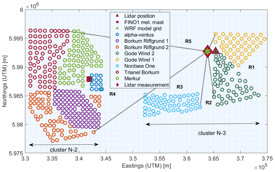
Figure 1 Location of the scanning lidar between the wind farm clusters showing the five sectors (from R1 to R5) into which the data are grouped for the analysis (dashed black lines). The individual wind turbines are represented by circles, and each individual wind farm is shown in a different color. The location of the meteorological mast FINO1 is also indicated (red square). The WRF model grid point investigated in this study is marked with a green star. Lidar system and lidar profile measurement locations are marked with a red triangle and a red diamond, respectively. Coordinates refer to UTM WGS84, zone 32.

A detailed description of the measurement methods can be found in the following sections. For the classification into the five different regions according to the wind direction, the actual position of the profile measurements at a distance of 1.5 km west of the scanning lidar device was used. From here, the positions of the outermost wind turbines of each wind farm cluster were used to limit the area as presented in Table 1. The regions R2 (south of the lidar location) and R5 (northwest) are not influenced by upstream wind farms. Region R1 (east) is influenced by the wind farms Gode Wind 1 and 2. Region R3 is influenced by the wind farm Nordsee One and region R4 by the wind farm cluster N-2 composed of the wind farms Trianel Borkum, Merkur, alpha ventus, and Borkum Riffgrund 1 and 2 (see Table 2 for a summary of the key characteristics of the wind farms surrounding the scanning lidar measurements).

Table 1 Ranges of the individual wind sectors (regions) and distances based on the measurement location of the scanning lidar system.

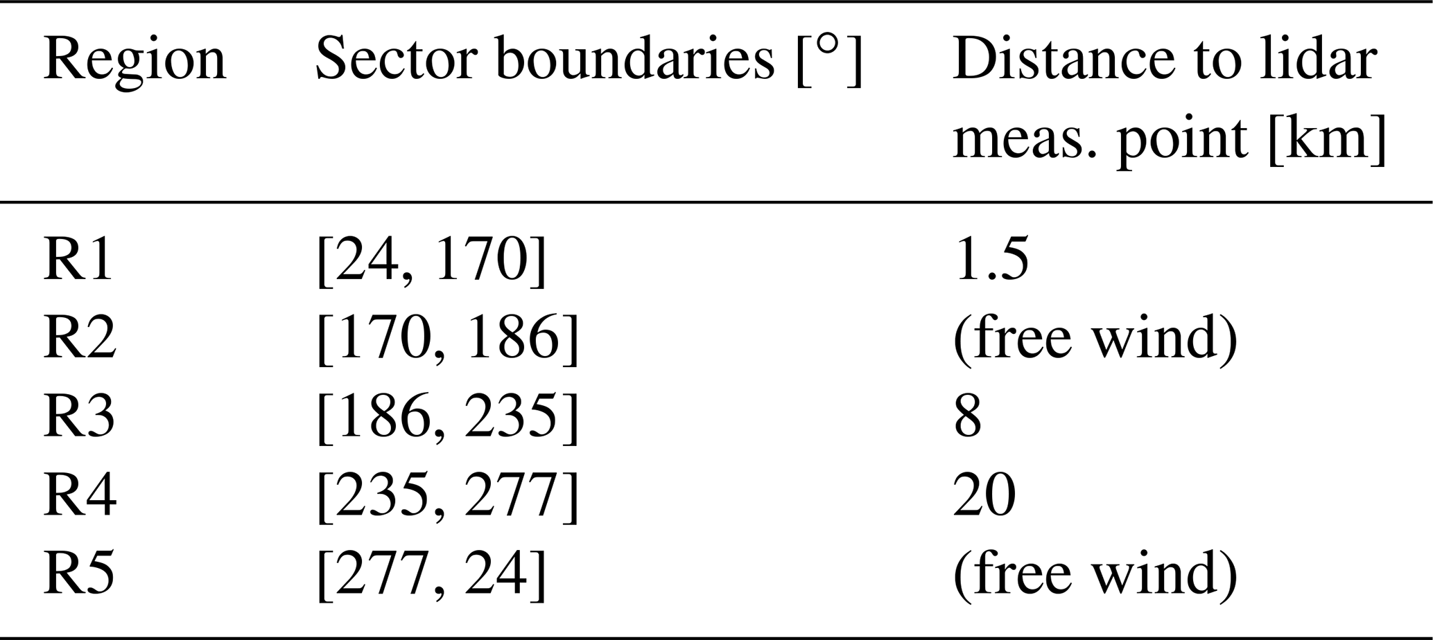
Table 2 Properties of the wind farms (as of May 2020) surrounding the scanning lidar measurement. The cluster name is defined by the German Federal Hydrographic Agency (), wind turbine (WT) type within the wind farms, WT rated power (P_rated), their rotor diameter (D), hub height (h) for LAT (lowest astronomical tide) and the number of wind turbines (No. of WTs).

After dividing the measurements into different regions based on wind direction, the lidar data have been further divided into subsets of atmospheric stability, which is expected to strongly affect the wind speed downstream due to the presence of far-field wind farm wakes (Cañadillas et al., 2020).

In this study, we use the static atmospheric stability, which only takes into account buoyancy effects and is characterized through the lapse rate (γ) based on the temperature gradient at two different altitudes, sea surface temperature (SST) and air temperature at the height of the transition piece (23.3 m) corrected for air pressure and density effects to obtain the virtual potential temperature (θ_v) gradient,

$$\begin{array}{}\text{(1)}& \mathit{\gamma }={\displaystyle \frac{\mathrm{d}{\mathit{\theta }}_{\mathrm{v}}}{\mathrm{d}z}}\approx {\displaystyle \frac{\mathrm{\Delta }{\mathit{\theta }}_{\mathrm{v}}}{\mathrm{\Delta }z}},\end{array}$$

with z the measurement height. Negative values of the virtual potential temperature gradient γ, or lapse rate, represent an unstable stratification of the atmosphere; positive values represent a stable stratification; and values around zero represent a neutral stratification. The stability classes were chosen as follows:

• $\mathit{\gamma }<-\mathrm{0.04}$: unstable stratification,

• $-\mathrm{0.04}\ge \mathit{\gamma }\le \mathrm{0.04}$: near-neutral stratification,

• γ > 0.04: stable stratification.

A thorough discussion of different parameters used to characterize stability and the influence on wakes is provided by Platis et al. (2021), who use similar values to classify atmospheric stability based on lapse rate. Ideally, it would be optimal to measure the air temperature at hub height or above, but due to the lack of measurements and considering that the air temperature measurements at the nacelle are highly biased due to the rotor effect, we consider our estimation to be suitable as a first-order approximation for the framework of this study.

2.1 Scanning wind lidar

Wind data were recorded with a long-range-scanning Doppler wind lidar system of the type Streamline XR manufactured by Halo Photonics, UK (METEK-GmbH, 2021). The lidar system emits short laser pulses into the atmosphere and detects the radiation backscattered by aerosols through optical heterodyning. This makes it possible to determine both the intensity of the backscattered radiation and its Doppler shift in the line-of-sight (LOS) direction, which is proportional to its radial wind speed, also called LOS wind speed.

The lidar system (see Fig. 2) was installed on the transition piece (TP) of the northernmost wind turbine (K01) of the wind farm Gode Wind 1, at a height of approximately 23.3 m LAT (lowest astronomical tide) and positioned on a metal support structure for a clear view in the azimuthal range [160^∘, 20^∘] over the railing to the west. In addition to the scanning lidar device, other sensors for collecting thermodynamic data (namely air temperature and humidity, pressure, precipitation, and water surface temperature) were installed. The purpose of these measurements was to characterize the atmospheric stability regime with the method previously described. The thermometer and hygrometer were mounted on a 50 cm long boom at a height of 22.5 m LAT, and the barometer was located in the control cabinet 50 cm below. The infrared sensor for measuring the SST was located on the railing of the TP and consists of a pair of sensors, with one sensor pointed towards the sea surface and the other towards the sky, which allows the temperature measurements to be corrected for the effects of background radiation (refer to Frühmann et al., 2018, for further details).

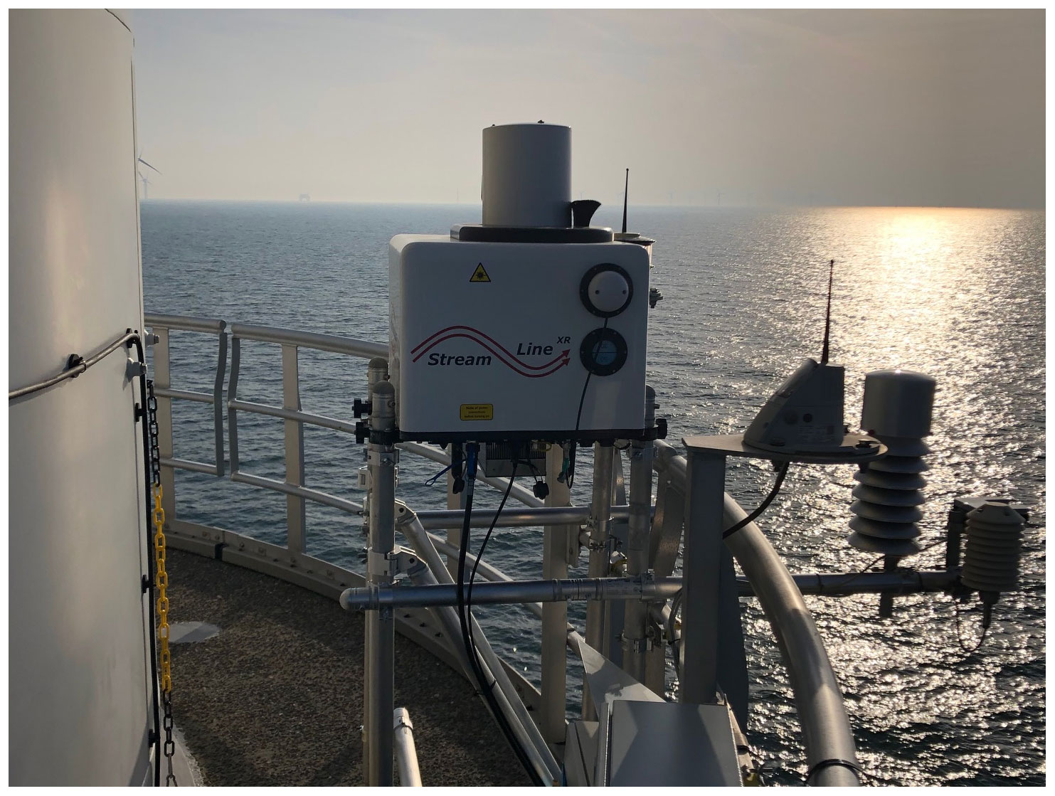
Figure 2 Long-range-scanning lidar and additional measurement systems (on the right side) on the TP of one of the northernmost wind turbines (K01) at the wind farm Gode Wind 1.

The lidar system, with a maximum range of 10 km, was set up with a gate length of 120 m. The sampling rate of the back-scattered signal of 50 MHz gives a spatial resolution of 3 m along the LOS. Furthermore, the accumulation rate can be reduced so that the highest beam sampling rate is 10 Hz. The laser beam is directed by a scanner with an arrangement of mirrors with 2 degrees of freedom, allowing scanning in all directions. The positioning of the scanner at the top of the lidar container box enables scanning of the sky above and a reduced area below the horizontal, without interference with itself.

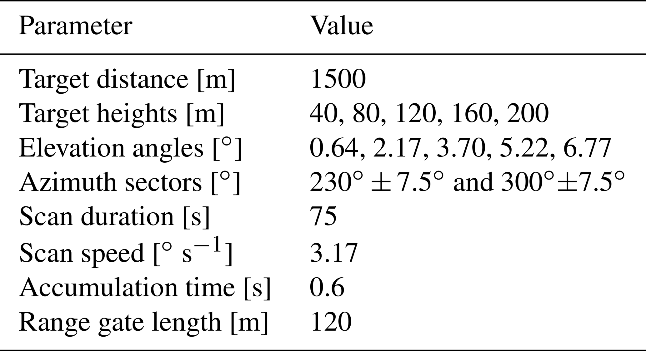
The lidar performed plan position indicator (PPI) scans (at five elevations) with continuous scanner movement in two azimuthal sectors of 15^∘ width upstream of the wind turbine K01. An overview of the lidar set-up is given in Table 3.

Table 3 Overview of scanning lidar set-up during the measurement campaign.

The set-up enabled the measurement of the wind profile in the vicinity of the wind farm Gode Wind 1 (approximately 1.5 km west of the wind turbine K01). To derive vertical profiles, we generate a so-called partial velocity azimuth display (VAD) plot at several altitudes using a sinusoidal function fitted to radial velocity data (Werner, 2005), which is represented as a function of azimuth. Then the results are calculated in terms of the Cartesian velocity components (u, v, w), and finally the wind speed and direction are derived. The classical approach relies on four radial velocities measured at constant elevation and in four quadrants in the azimuth around the lidar. In our approach, we rely on several radial velocities measured continuously on a limited area in azimuth and constant elevation to avoid measurements influenced by the wake of the wind farms Gode Wind 1 and 2. The general sketch of the approach in Fig. 3a shows how data are selected for the VAD plot near a target point and for several heights (panel b). After selecting data for an altitude, a check is made to see if the data meet a minimum carrier-to-noise ratio (CNR), and then a sine function is fitted using random sampling consensus (RANSAC) (Fischler and Bolles, 1981). This last method is used to avoid the remaining outliers and to increase the robustness of the fitting procedure.

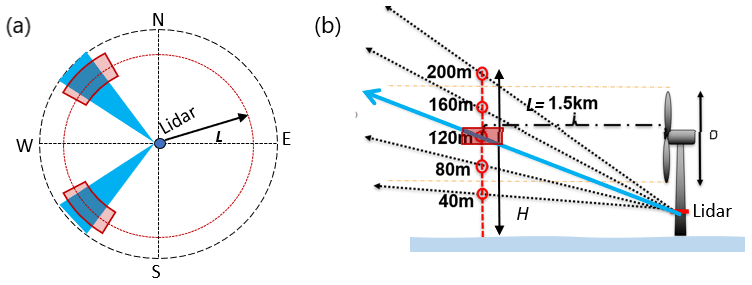
Figure 3 (a) Sketch of scanning for partial VAD. Shaded areas in blue represent areas where the wind is interrogated continuously. Areas in red represent the volumes where data for VAD are selected. (b) Sketch of the vertical profile of the wind speed and wind direction at the five target heights selected in this campaign, where L is the distance from the lidar system to the measurement location.

As the lidar was positioned west of Gode Wind 1, the scanning was performed to the western side, targeting five heights above LAT, namely at 40, 80, 120, 160 and 200 m. In this free sector, we followed the scanning trajectory shown in Fig. 4a and with the scanner set-up shown in Table 3. In Fig. 4b, an example of the VAD results for the wind speed and wind direction for 1500 m and a height of 120 m is shown. In practice, every time a scan is finished, i.e., every 75 s (see key scanning parameters in Table 3), a VAD is performed and wind speed and wind direction at all five heights are stored. Finally, these data are averaged over 10 min.

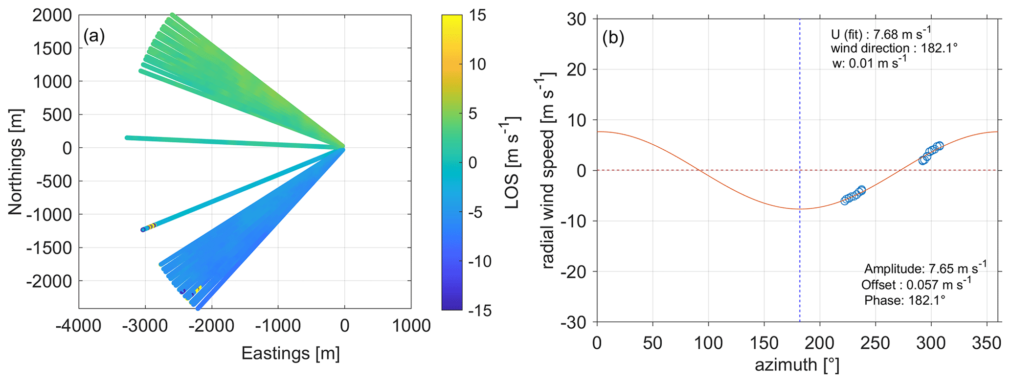
Figure 4 (a) Example of the top view of the radial wind speed (u_r) for a single full scan taking approximately 75 s on 29 August 2020. Eastings and northings are given in meters and relative to the lidar position. (b) Example of VAD data selected from the scan in (a) for a distance of 1500 m ±150 m and a height of 120 m ±5 m. The bottom legend shows results for the radial wind speed fit. The top legend indicates results of the wind speed.

An important point to consider when measuring wind with a lidar system is the orientation of the system. Orientation errors in the scanning lidar affect the exact position at which the wind is interrogated by the laser beam. Three angles are used to fully define the orientation of the lidar in three-dimensional space, namely bearing, tilt and roll. The further the distance to the lidar, the larger the error in positioning is, due to errors in one of these angles. It is therefore necessary to determine these angles at very high accuracy in order to reduce and properly quantify the positioning uncertainty. While the offset in the azimuthal direction between the geographic north and the lidar's north mark can be determined with a compass, this is very inaccurate for the site installation because the turbine structure affects the magnetic field around the lidar. A better option is to use the lidar itself and neighboring turbines of which their position is known (“hard targeting”). In this study, we target turbines of the neighboring wind farm Nordsee One at distances between 8 and 10 km and identified them by their very high backscattered signal with an accuracy of at least 0.1^∘. In addition, the system is equipped with an internal inclinometer, which is used to quantify tilt and roll. However, the manufacturer does not provide calibration information for this sensor. Furthermore, due to the high relevance of these angles, it is desirable, if not mandatory, to perform an on-site assessment of mounting errors and inclinometer performance. For this purpose, we apply the so-called sea surface leveling (SSL) proposed by Rott et al. (2022) during the commissioning of the lidar system at the offshore site. In this procedure, the sea surface is used as a reference to assess the orientation of the lidar system relative to the horizontal plane. Mainly, the scanning lidar, which is installed several meters above the sea, is set to perform a scan with constant downward elevation and constant azimuth velocity. In this set-up, the backscattered lidar signal describes the surface of a cone that extinguishes by absorption as it enters the water. The geometric analysis of the elliptical shape of the intersection of the cone with the water surface (see Fig. 5) provides the tilt and roll angles of the cone axis and thus of the lidar itself.

Figure 5 Example of backscattered signal intensity after SSL scanning. Red dots show the estimated water entrance. The red ellipse and its axes reveal a misalignment of the sensor. The blind area to the east is due to the turbine tower.

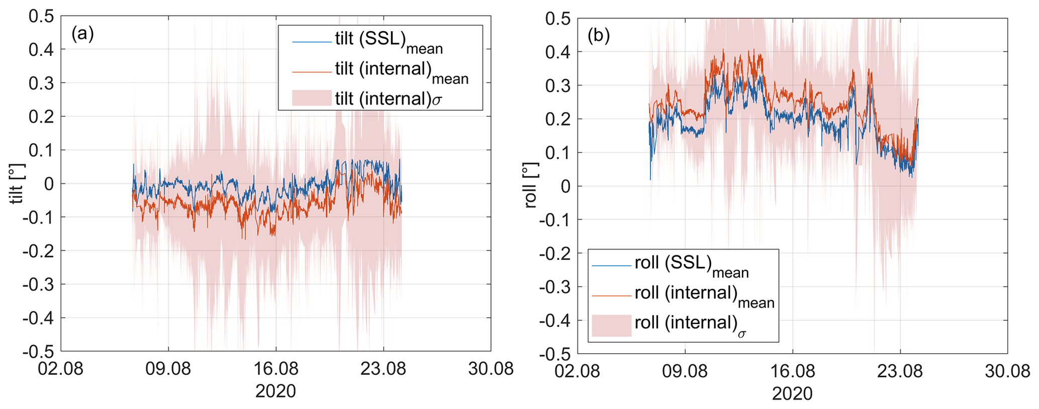
Figure 6 (a) Lidar tilt from internal inclinometer (internal, red) and from SSL (blue). The red band shows the standard deviation (SD) of the inclinometer tilt during each SSL scan. (b) Lidar roll from internal inclinometer (internal, red) and from SSL (blue). The red band shows the standard deviation (σ) of the inclinometer roll during each SSL scan.

We adopt the results of the SSL method as a reference because they show the misalignment of lidar, scanner and support structure combined in a direct way. For this reason, the misalignment results from the SSL can be used in trajectory planning. Eventually, the data could also be used to calibrate the internal inclinometer or any other auxiliary inclinometer used in a campaign. The SSL is performed regularly to check if the alignment has changed.

To assess the robustness of the SSL and its performance against the internal inclinometer of the scanner system, we ran the SSL continuously for almost 18 d from 6–24 August 2020. Figure 6a and b show, respectively, the time series of tilt and roll obtained from the SSL and the internal inclinometer. Each time step represents the result of a full SSL scan (with a duration of about 2.5 min) and the corresponding mean value of the inclinometer data. In addition, the standard deviation of the inclinometer is shown as a band of ±σ. The results show a good correlation between the two signals. The SSL indicates a different bias in each axis of the inclinometer, namely tilt${}_{\mathrm{bias}}=-\mathrm{0.05}{}^{\circ }$ and roll${}_{\mathrm{bias}}=+\mathrm{0.05}{}^{\circ }$. A change in mean tilt and roll over time can be observed. This is due to the varying conditions of the support structure. In particular, the thrust of the wind turbine changes the magnitude and direction of the tower inclination depending on the wind direction and wind speed. The error between the two sensors (now assuming SSL as the sensor) can be seen in Fig. 6a and b. After debiasing both errors, we obtain mean-square errors of ${\mathit{ϵ}}_{\mathrm{tilt}}=\mathrm{0.01}{}^{\circ }$ and ${\mathit{ϵ}}_{\mathrm{roll}}=\mathrm{0.02}{}^{\circ }$. Finally, the variance of the inclinometer is a consequence of the system dynamics, which must be taken into account when assessing the accuracy of the scanner alignment. The total variance of the inclinometer signals is ${\mathit{\sigma }}_{\mathrm{tilt}}=\mathrm{0.23}{}^{\circ }$ and ${\mathit{\sigma }}_{\mathrm{roll}}=\mathrm{0.24}{}^{\circ }$. It should be noted that in the absence of information on the calibration of this sensor, we assume this value to be conservative. This is based on the assumption not only that the sensor perfectly detects rotational changes but also that the resulting values are a superposition of rotational and translational movements.

2.2 Mesoscale model

Mesoscale simulations, including both undisturbed free wind conditions and the wake-disturbed wind field due to the surrounding wind farm, were performed using the WRF model (version 4.2.1) developed by the National Center of Atmospheric Research (Skamarock et al., 2019). In the WRF model, there are prognostic variables for the horizontal and vertical wind components, potential temperature, geopotential and surface pressure of dry air as well as several scalars such as cloud water and water vapor. The WRF model is well known and widely used in the wind energy community (Huang et al., 2014; Hahmann et al., 2020; Kibona, 2020), and in recent years also for wind farm wake simulations (Pryor et al., 2019; Siedersleben et al., 2018b).

Our set-up was optimized within several research projects for wind energy applications, especially with a focus on offshore conditions (Gottschall et al., 2018; Dörenkämper et al., 2020; Gottschall and Dörenkämper, 2021). The studies by Gottschall et al. (2018) and Gottschall and Dörenkämper (2021) compare the mesoscale model data from a similar set-up against vertical lidar and mast measurements. The WRF model set-up is based on the extensive sensitivity studies carried out in the framework of the NEWA (New European Wind Atlas) project (Hahmann et al., 2020; Dörenkämper et al., 2020). The final set-up was validated against almost 300 masts in different terrain complexity. In low terrain complexity this set-up showed a bias of the mean wind speed of 0.06 m s⁻¹ ± 0.49 m s⁻¹ evaluated at 110 masts. To limit the number of grid points in the numerical calculations, a nesting technique is used. Three domains centered around the German Bight area are nested, each of a size of 120 grid points with resolutions of 18, 6 and 2 km. Figure 7a shows the distribution and size of the three domains around the site of interest.

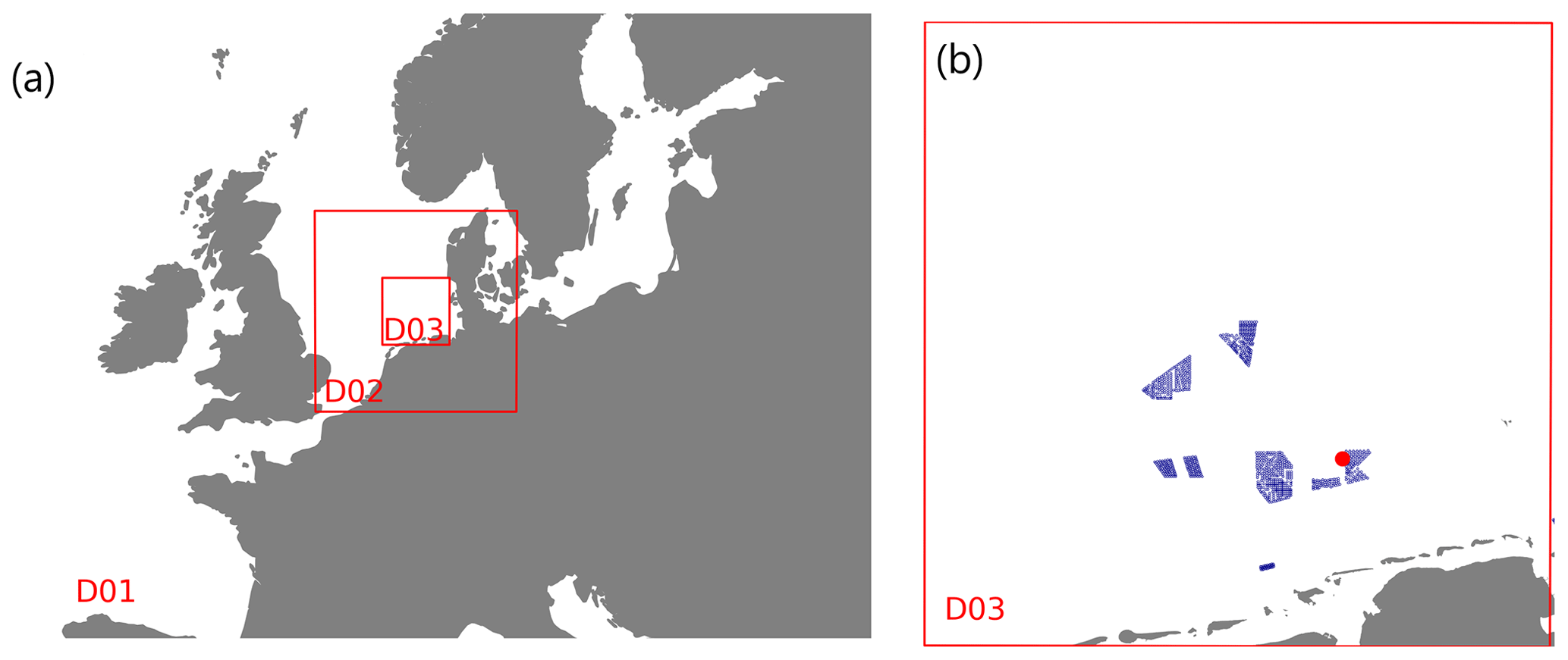
Figure 7 (a) Locations of the three WRF model domains (D01, D02, D03) with a grid sizes of 18, 6 and 2 km, respectively. The innermost domain (D03) of (a) is shown in detail in (b) with the locations of the wind turbines accounted for in the simulations and the location of the lidar measurements marked in red. Note that wind farms with a distance of more than 100 km from the site were ignored.

The wind turbines were parameterized as momentum sinks and source of turbulence using the Fitch wind farm parameterization (Fitch et al., 2012). In every grid that intersects the rotor disk, the horizontal wind components are reduced to represent the drag of the wind turbine. Different thrust and power curves corresponding to all turbine types were applied. Figure 7b shows the locations of the turbines in the model simulations. Boundary conditions for the model were prescribed by the ERA5 dataset (ERA5 resolution, $\mathrm{0.25}{}^{\circ }\times \mathrm{0.25}{}^{\circ }$ (∼30 km), 6-hourly) for the atmospheric variables (Hersbach et al., 2020) and the OSTIA dataset for the sea surface variables (Donlon et al., 2012), which provides near-real-time global sea surface temperature at the grid resolution of $\mathrm{1}/\mathrm{20}{}^{\circ }$ (∼6 km). The WRF version used in this study does account for the turbulent-kinetic-energy advection bug that was recently discovered (Archer et al., 2020).

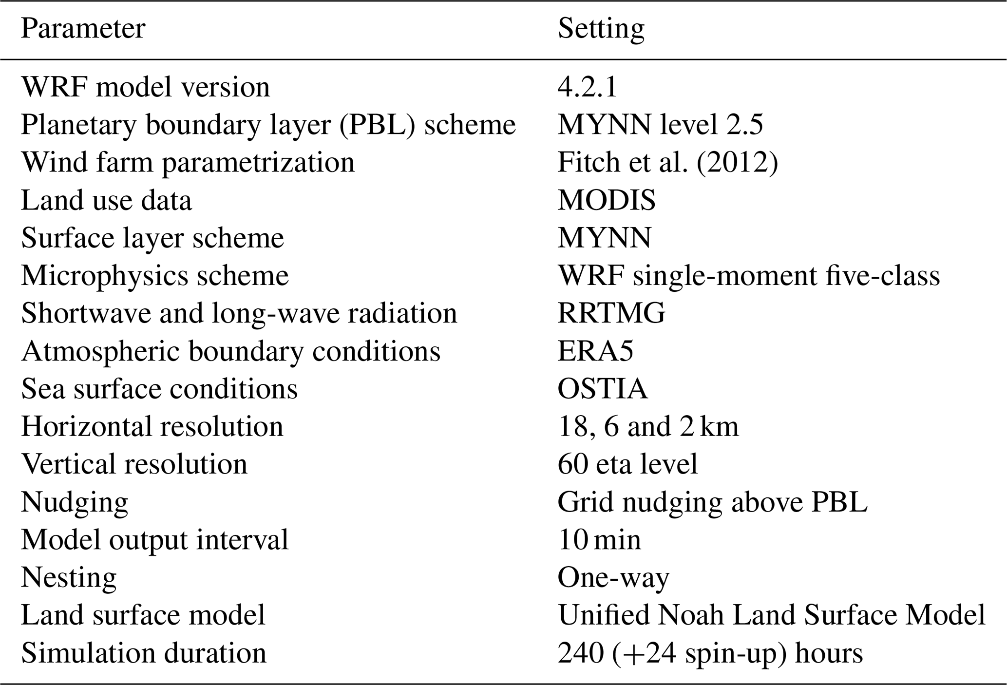
We performed simulations with and without wind farms and extracted the time series from the WRF simulations at the position of the scanning lidar measurements for the same period. The most important settings of the mesoscale model configuration are summarized in Table 4.

Fitch et al. (2012)

Table 4 Relevant parameters of the mesoscale model set-up. The references for the different schemes and models are summarized in WRF Users Page (2020).

2.3 Airborne measurements

The spatial extent of the wind farm wakes can be briefly investigated by considering one of the measurement flights carried out during the scanning wind lidar measurement period with the research aircraft Dornier DO-128 operated by the Technische Universität Braunschweig (Lampert et al., 2020).

Although the flight data are limited to a few hours within a single day, they provide an overview of the wind situation at different distances and vertical profiles both upstream and downstream of the wind farm clusters. The research aircraft is equipped with a nose boom to perform high-resolution measurements of the wind vector, temperature, humidity and pressure, sampling at a frequency of 100 Hz (Corsmeier et al., 2001). Sensors for measuring the surface temperature, a laser scanner for determining sea state characteristics and cameras were also integrated (Lampert et al., 2020). During the measurement flights, both the upstream and downstream areas of the wind farm clusters were investigated. The flight pattern included legs of 45 km length that were aligned perpendicular to the main wind direction, therefore crossing the wakes, and vertical profiles from around 15 m altitude up to 1000 m. The individual straight flight legs were horizontally spaced about 10 km from each other. The measurement height was 120 m above sea level, which corresponds to the hub height of the wind farms Gode Wind 1 and 2.

An example of a flight dataset showing multiple wake-transect profiles perpendicular to the mean wind direction, measured downstream of clusters N-2 and N-3 on 3 July 2020, is briefly presented in the next section.

3 Wind field modification by wind farm clusters

The strong modification of the wind field by the wind farm clusters is clearly evident in scanning lidar measurements, flight measurements and WRF simulations. Flight measurements enable an initial side-by-side evaluation of the WRF model over a larger spatial scale than is possible with just the scanning lidar system and illustrate the strength and extent of wind farm cluster wakes (Sect. 3.1). The lidar measurements are then compared with WRF model results with and without a wind farm parameterization for the different sectors and atmospheric stability conditions, which enables an evaluation of WRF performance for different upstream wind conditions (Sect. 3.2).

3.1 The spatial extension of cluster wakes

Because of the extended range of flight paths around the wind farm clusters, the flight measurements are presented here to complement the lidar measurements. We consider the wake situation of the N-2 and N-3 clusters on 3 July 2020 (10:24–13:02 UTC) when flight legs were performed perpendicular to the mean wind direction ($\approx \mathrm{230}{}^{\circ }$) and taking on average 10 min per traversal. The cluster wake limits in Fig. 8a are defined as the physical cluster extent which expands with distance x at the rate of k_w=0.04 (wake decay constant for offshore as suggested by Sørensen et al., 2008.

The spatial distribution of the measured wind speed is inferred in Fig. 8a from the flight legs extending perpendicular to the wind direction. Darker colors, representing lower wind speed values, are evident directly behind the wind farms and more dense clusters of wind turbines. In particular, the strong reduction in wind speed downstream of cluster N-2, which is located to the west, but also the wind farms Gode Wind 1 and 2, which are located further to the east, can be clearly seen. Behind the northeastern edge of Gode Wind 2, the wind speed is about 7.5 m s⁻¹. Upstream of the wind farm, the wind speed is about 11 m s⁻¹, which corresponds to a reduction in wind speed of about 30 %. Stability during this period was inferred from vertical temperature profiles outside the wake area influenced by the wind farm clusters by steep climbing and descending flight profiles up to an altitude of about 1000 m, which reveal, after an initial close-to-neutral period (−0.005 K m⁻¹), stable conditions (with a maximum value of 0.01 K m⁻¹) for the last legs and thus explain the strong wakes detected.

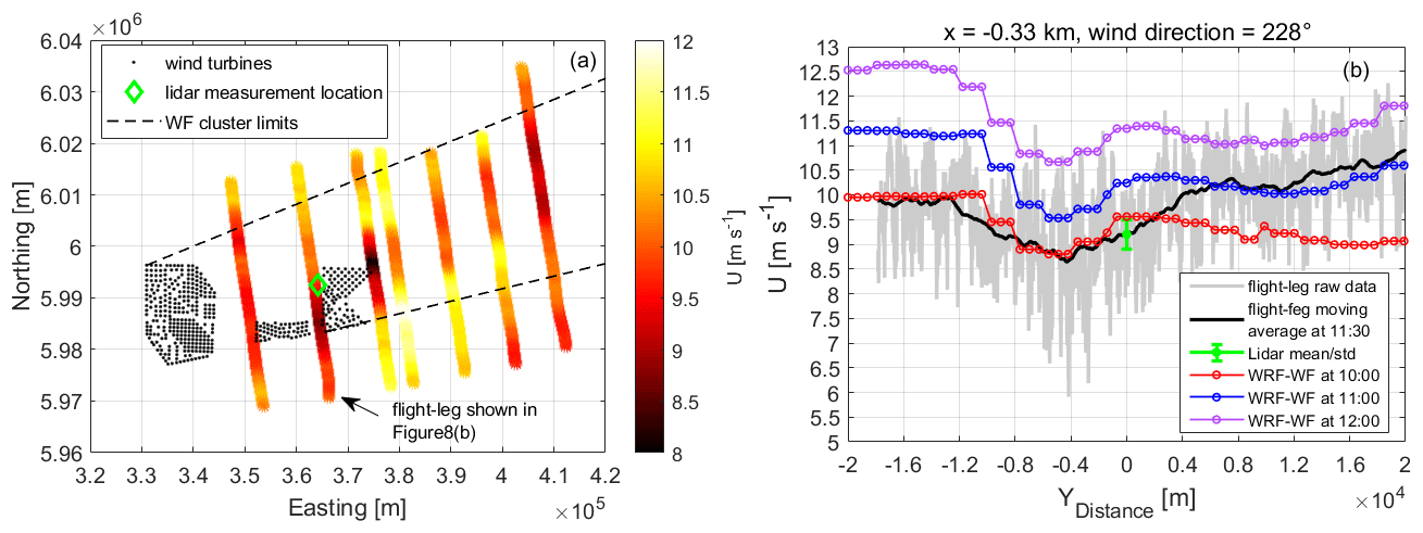
Figure 8 (a) Flight path in the vicinity of the clusters N-2 and N-3 (individual turbines as black points) of the measured wind speed from the measurement flight on 3 July 2020 (10:24–13:02 UTC). The black dashed lines indicate the downstream boundaries of the clusters for the measured wind direction of 230^∘. The flight altitude during the traversals of the wake clusters was ≈120 m, and the coordinates refer to UTM WGS84, zone 32. (b) Horizontal wind speed transect for the closest flight traversal upstream of the lidar measurement point ($x=-\mathrm{0.33}$ km, where the negative sign refers to the left of the location of the measurements obtained by scanning lidar) and perpendicular to the wind direction. The gray line represents the 100 Hz data, the black line shows the data filtered by a moving average and the green diamond with error bars represents the lidar mean wind speed and its standard deviation for the duration of the flight leg (≈10 min). The red, blue and purple dotted lines show the WRF results with a wind farm parameterization (WRF-WF) from a transect of the model results at 10:00, 11:00 and 12:00 UTC, respectively, based on the flight coordinates.

Figure 8b shows the horizontal wind speed transect for the closest flight traversal (black line) upstream of the lidar measurement point ($x=-\mathrm{0.33}$ km) compared with the mean wind speed according to the lidar (green diamond) and standard deviation for the duration of the flight leg (error bars), revealing a suitable agreement between the two measurements for this flight (mean bias = 0.06 m s⁻¹). For this leg, the lapse rate was −0.003 K m⁻¹, implying neutral conditions, which explains the relatively high turbulence signal in the 100 Hz data (gray line). The flight leg was performed between 11:27 and 11:37 UTC.

For comparison, the WRF-WF model results for the times 10:00 (red dotted curve), 11:00 (blue dotted curve) and 12:00 (purple dotted curve) UTC are shown for a transect corresponding to the flight coordinates. Note that for this particular time period, there is an approximate time delay of around 1 h, which is common in WRF results. The flight altitude corresponds to approximately 120 m, corresponding to the mean hub height of the N-2 and N-3 clusters and the mean wind direction of 228^∘ for this transect. While these data also show a decrease in the wind speed between the limits of the cluster N-2, the wind speed of the wake minimum is about 0.5 m s⁻¹ higher than the flight leg. The mean wind direction difference between the flight leg and the simulation is about 10^∘. It is worth mentioning that the WRF simulation does not take into account the wind farms located at about 15 km east of the cluster N-2 (Gemini wind farm), which could explain the difference of more than 1 m s⁻¹ at the northern part of the wind farm wake (negative x axes).

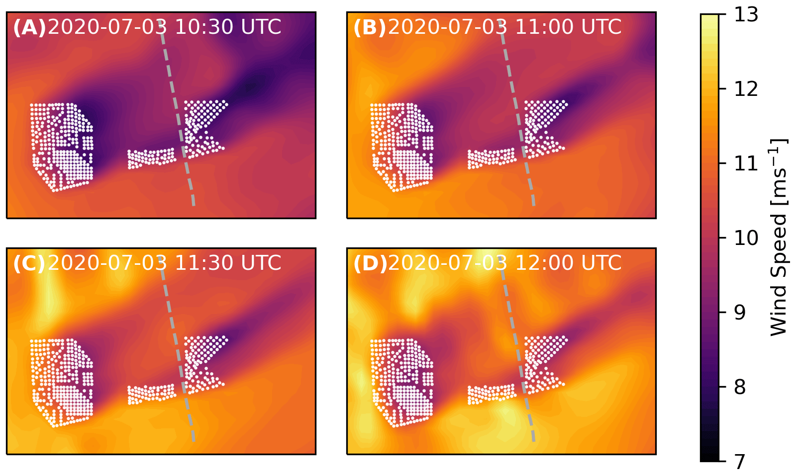
Figure 9 shows the WRF-model-simulated horizontal wind field with the wind farm parameterization at mean hub height (120 m) and at different time steps.

Both the observations (Fig. 8a) and model (Fig. 9) show a wake extending at least 40 km downstream of the N-3 wind farm cluster, meaning this wake was long enough to reach the wind farm cluster N-4 (not shown) located about 60 km downstream of Gode Wind. In the spanwise direction, the wake has dimensions of approximately the maximum width of the wind farms. The simulations for different time steps indicate the temporal variability of the wind field well, which has to be considered for a flight duration of 4 h as well. As shown next, significant wake effects were detected by the scanning lidar for cases such as these for flow from the east.

Figure 9 Spatial distribution of the modeled wind speed (see color bar) from the WRF simulation with a wind farm parameterization on 3 July 2020 at different time steps. The dashed gray line indicates the position of the flight leg shown in Fig. 8b.

3.2 Directional and stability dependence of cluster wakes

We evaluate the lidar-derived wind speed measurements by first dividing the wind direction into five unequal sectors within the cluster wakes (see Fig. 1). The lidar measurements are then compared with mesoscale model results without and with a wind farm parametrization for the different sectors, which enables (1) an estimation of the wind speed deficit when using the model without wind farm parametrization and (2) an evaluation of the model (with wind farm parametrization) performance for the different upstream conditions. Note that because the stability is also wind direction dependent at this site, some sectors are affected more by certain stability conditions.

Figure 10a shows the wind rose from the lidar measurements together with the five wind direction regions R1–5, illustrating the predominance of a west-southwesterly wind direction for the data period presented here, which corresponds to the main meteorological wind direction in the German Bight area (Cañadillas et al., 2020). Figure 10b shows the Weibull distribution for the wind speed together with the scale parameter A and shape parameter k for each region R1–5 at 120 m. This illustrates that meteorological conditions and wind speed distributions within a region are very different, so that a direct comparison of wind data between the different sectors does not make sense due to the different flow conditions found in each sector. (For a more detailed depiction of the lidar data distribution for different sectors, please refer to Appendix B.)

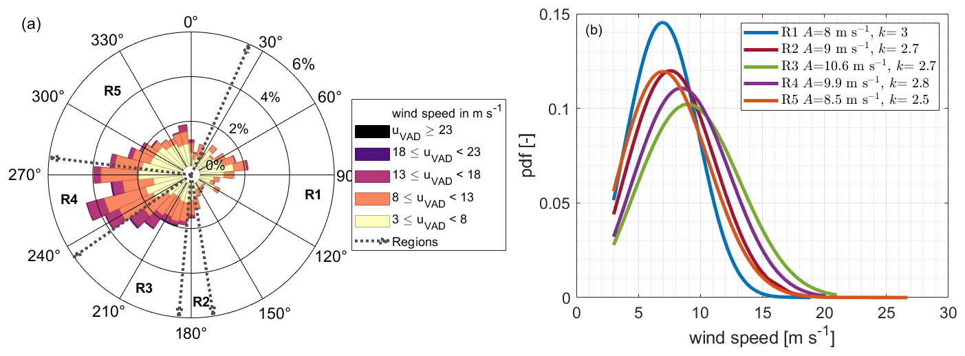
Figure 10 Wind rose (a) and Weibull distribution per regions R1–5 (b) at 120 m altitude measured by the scanning wind lidar for the period from May to September 2020.

The wind roses derived from lidar data for different atmospheric stabilities are shown in Fig. 11, illustrating that a large part of the data obtained during stable atmospheric stratification correspond to flow from the east. With neutral atmospheric stability, southwesterly winds prevail, while in unstable stratification northwesterly winds are predominant. Unstable and neutral conditions are associated with higher average wind speeds than stable conditions.

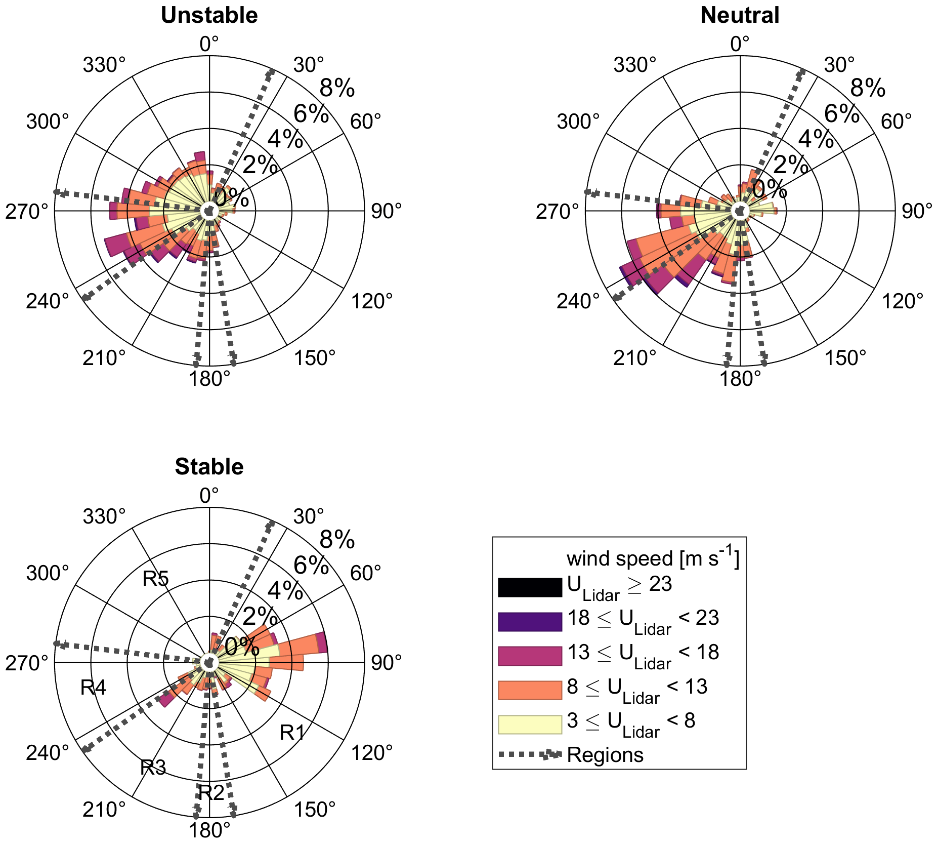
Figure 11 Wind roses measured by the scanning lidar for different atmospheric stabilities at 120 m above LAT. The regions R1–5 are indicated by dashed lines.

The wake-induced wind speed reduction at the position of the lidar measurements is investigated for each wind region using a polar plot for which the mesoscale simulation results (without wind farm parameterization) are used as the reference free wind speed. Since the model data represent an undisturbed state not influenced by wind farms, differences in the wind conditions are to be expected when comparing the two datasets. Especially in the regions R1, R3 and R4, which are directly influenced by the wind farm clusters, lower measured wind speed values are expected. Figure 12 shows the direct comparison of the wind speed values per wind direction of the lidar and the mesoscale model data at 120 m height for (a) unstable, (b) neutral and (c) stable atmospheric conditions. To aid visualization, the boundaries of the regions R1 to R5 and the individual positions of the wind turbines are also indicated.

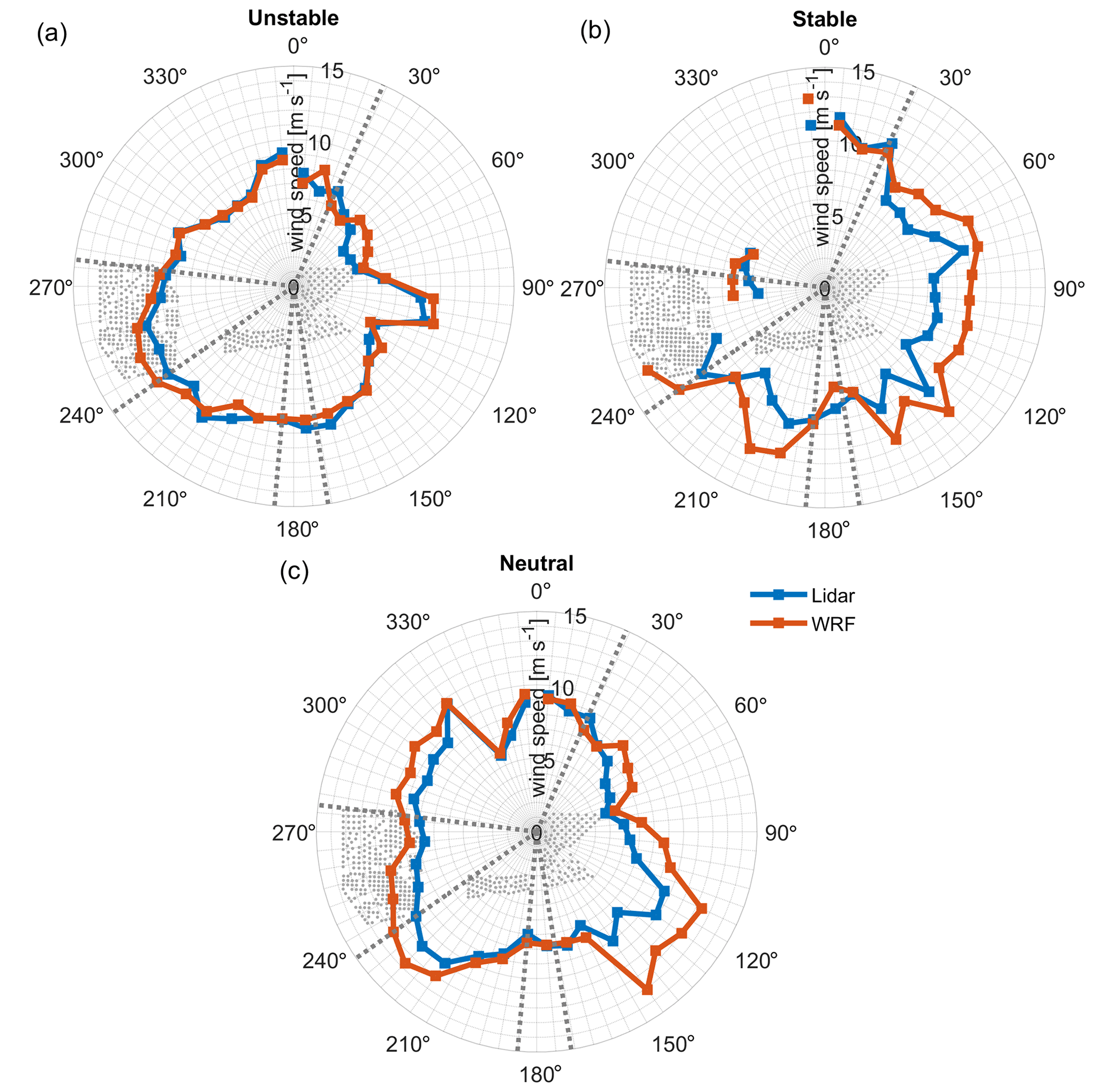
Figure 12 Wind speed polar plots of the lidar measurements and WRF results (without the wind farm parameterization) for (a) unstable, (b) stable and (c) and neutral atmospheric stratification at the height of 120 m. Wind turbines are indicated by gray points and the regions R1–5 by dashed gray lines.

Relatively good agreement is found between both datasets in unstable conditions and in region R2 in neutral conditions. The difference in wind speed in the other regions is also minimal under unstable stratification where the influence of the wind farms is difficult to detect in the measurements since wind farm wakes are not expected to be large. In contrast, a comparison of the datasets for neutral and stable atmospheric stratification shows a clear discrepancy between the measurements and model results, with this difference particularly evident in the regions R1, R3 and R4, which are directly influenced by wind farm clusters. The maximum difference is about 4 m s⁻¹ in region R3 in stable stratification. Even with neutral stratification, a difference can be seen in the two wind speed datasets and the regions influenced by wind farms. In the free-wind region, however, both datasets agree very well. The strong fluctuations in the wind speed of the lidar data in region R1 are due to the very small amount of data in neutral stratification (see Fig. 12). For region R5, in the case of stable atmospheric stratification, there are no or too few data available in some wind direction sectors. A comparison of the data from the free-wind sector is not possible here. Nevertheless, the reduction in wind speed caused by the wind farms in the other regions can be clearly seen.

To quantify the effects of the wind farm wake in the different regions, the wind speed deficit (ϵ_WRF) of the lidar-measured wind speed u_lidar with respect to the mesoscale wind speed u_WRF is defined as

$$\begin{array}{}\text{(2)}& {\mathit{ϵ}}_{\mathrm{WRF}}=\left({\displaystyle \frac{u_{\mathrm{lidar}}}{u_{\mathrm{WRF}}}}-\mathrm{1}\right)\mathrm{100}\mathit{\%}\end{array}$$

and presented in Fig. 13a, which is computed as an average over all points in each wind direction region for unstable, neutral and stable conditions. The bars within a group represent the five measurement heights of 40, 80, 120, 160 and 200 m, and the number of 10 min lidar values within a bar is shown at the end of the bar.

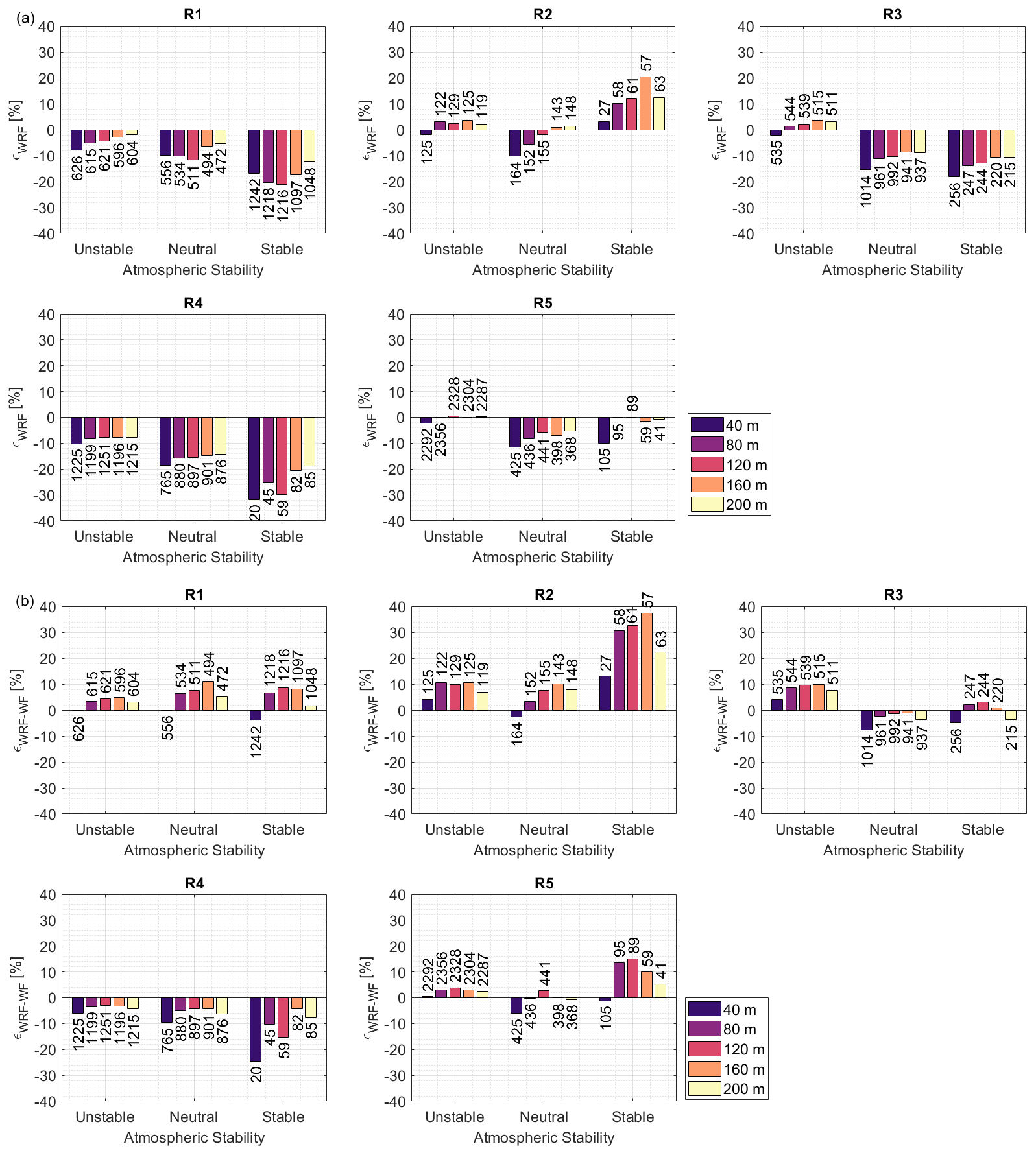
Figure 13 The deficit ϵ_WRF (Eq. 2) in the wind speed between the lidar measurements and WRF model for (a) no wind farm parameterization u_diff(WRF) and (b) with the wind farm parameterization ϵ_WRF-WF for regions R1 to R5; for each measurement height 40, 80, 120, 160 and 200 m; and for each stability class. The number below and above each bar indicates the number of 10 min wind speed values.

The wind speed deficit ϵ_WRF in region R5, the free-wind region, is small for neutral and unstable conditions (<10 %), especially for unstable stratification (1 %–2 %), for all measurement heights. For the second free-wind sector R2, only small differences between the WRF model and lidar data are evident in the case of unstable and neutral atmospheric stratification. However, the results in this sector vary strongly with height. One possible reason for this is that the lateral extent of the narrow undisturbed corridor in region R2 is too small, only about 3 km, and that the boundaries of the wake effects become wider with increasing distance to a wind farm due to the wake expansion. This effect is enhanced by a stable atmosphere. Even when the corridor was further narrowed by changing the region boundaries of R2, no effect similar to R5 was detected. The small horizontal extent of the corridor and the large distance of the lidar measurement site from this area make a differentiated evaluation of region R2 difficult.

The regions R1, R3 and R4 influenced by the wind turbines all show a relatively large wind speed deficit. As expected, the ϵ_WRF values measured are generally lower (negative) than the values from the undisturbed computational model at all heights and stability conditions, particularly in stable stratification. In region R4 and at a measurement height of 120 m, ${\mathit{ϵ}}_{\mathrm{WRF}}\approx -\mathrm{30}\mathit{\%}$ in stable stratification. It is also noticeable that the reduction in wind speed shows a negative trend with increasing height. While the maximum height of the lidar measurements may be 200 m and most of the wind turbines in the surrounding area have a total height between 140 and 180 m, some interaction effects can also be detected above the wind farm due to vertical wake expansion (Siedersleben et al., 2018a; Larsén and Fischereit, 2021). However, as measurements at a height of 200 m are only partially influenced by the wind turbines, as they are no longer completely behind the rotor surface, this probably explains the lower wind speed deficit at 200 m.

The wind speed differences can be further emphasized for different atmospheric stability conditions within a region. Here it is noticeable that, in regions R4 and R3, a strong reduction in wind speed behind the wind farms with increasing atmospheric stability can be seen, but this is much less pronounced in region R1. As regions R3 and R4 have a larger distance to the measuring point of the lidar than region R1, it can be assumed that, in an unstable atmosphere, the wind speed recovers more quickly in the wake of a wind farm than in stable conditions, as also shown in Cañadillas et al. (2020).

The lateral extent of a wind farm, i.e., the number of wind turbines in the flow direction as well as the wind turbine layout, also affects the strength of the change in wind conditions in the wake of a wind farm cluster. Region R3 is influenced by the wind farm Nordsee One. Here, a maximum of six to seven wind turbines are located behind each other in the flow direction. In region R4, which is influenced by the wind farm cluster N-2, the number of wind turbines in the direction of flow is 17 to 20 turbines, depending on the wind direction. This effect is evident when considering the wind speed differences in regions R3 and R4 under unstable atmospheric conditions. Although the distance of the wind farm in region R3 to the measurement location of the lidar is significantly smaller, the reduction in wind speed is smaller than in region R4. A possible reason for this is the size of the wind farm cluster in R4.

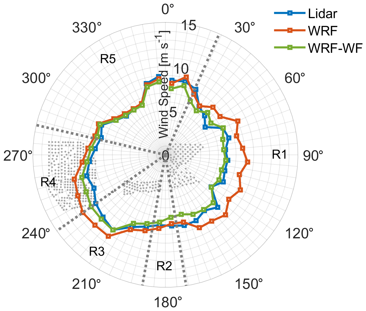
Figure 14 Wind speed polar plot of the lidar (blue) and WRF model without (red) and with wind farm influences (WRF-WF, green) at 120 m. Wind turbines are indicated as gray points, and the sectors are indicated as dashed gray lines.

Figure 14 shows a polar plot comparing WRF results, both without and with wind farms, with the lidar measurements, for all atmospheric stabilities detected during the measurement period. To ensure a fair comparison between the mesoscale (WRF-WF) model and the lidar, hourly production data from energy charts (available at https://www.energy-charts.de/, last access: July 2021) were used for filtering purposes. Only wind farms in operation at the measurement times are included in the mesoscale simulations and thus considered in the comparison.

Wind speed deficits of up to about 30 % are shown for the easterly winds at a distance of 1.5 km and up to 15 % for the southwesterly flow at a distance of about 20 km. On the other hand, the lidar (blue) and WRF-WF (green) data show improved agreement between the two datasets for all directions with a difference in wind speed of about 2 %, indicating that the WRF-WF model with the wind farm parameterization included is capable of capturing the mean wake effects detected by the in situ measurements.

As for Fig. 12, the data presented in Fig. 14 are divided into unstable (a), stable (b) and neutral (c) conditions in Fig. 15 for the WRF model with the wind farm parameterization (green line) and for the scanning lidar (blue line). A good agreement is found for most of the regions (R1, R4 and R5) under unstable conditions with a wind speed difference of around 2 % in wind speed. The larger disagreements in wind speed (almost 15 %–20 %) are found under stable conditions for the regions R1 (downstream of the large wind farm clusters Gode Wind, N-2) and R2 and of around 10 % for the region R3 (downstream of the relatively small wind farm Nordsee One).

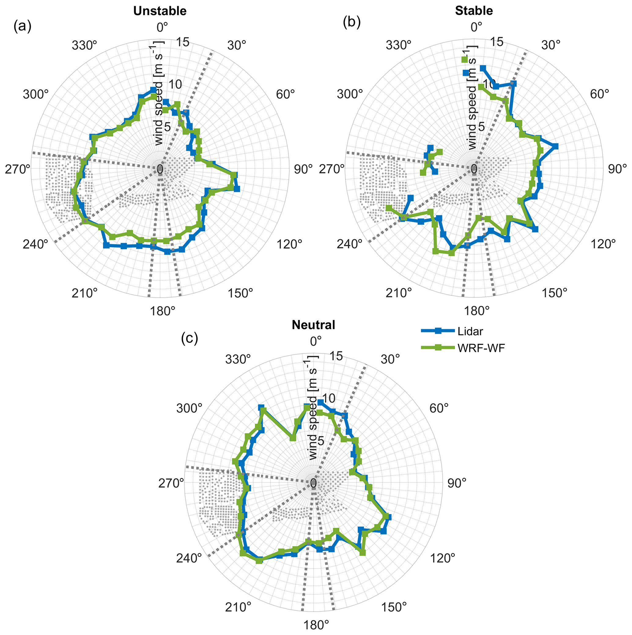
Figure 15 Wind speed polar plots of the lidar measurements and WRF-WF results (with the wind farm parameterization) for (a) unstable, (b) stable and (c) neutral stratification at the height of 120 m. Wind turbines are indicated by gray points and the regions R1–5 by dashed gray lines.

Figure 13 (lower panels) also presents the wind speed difference for the mesoscale model ϵ_WRF-WF. In general, the wind farm parameterization reduces the absolute magnitude of the wind speed difference ϵ_WRF-WF in the waked regions, especially for regions R1 and R4 to, respectively, the east and west of the lidar for all stability classes, and for region R3 to the southwest of the lidar, except for unstable conditions where the value of ϵ_WRF-WF is more positive for all heights. This could be due to coastal effects to the south not being properly captured by the model (see also the southern part of the polar plot in Fig. 15a). The difference in the narrow region R2 to the south is also worsened by the wind farm parameterization, including for all stability classes. Our lidar measurements thus serve as a reference for further improvements in wind farm parameterizations.

4 Discussion

In this study measurements of wakes inside an offshore cluster are reported for the first time. Data of a lidar scanner installed on the transition piece of a wind turbine located within a cluster in the German Bight are collected and analyzed within a 5-month field campaign. As part of the goals of this study, a detailed description of the experimental set-up and an uncertainty estimation have also been presented. We have implemented a method for obtaining a representative wind speed vertical profile with a single scanning lidar for areas nearby offshore wind farms. The method comprises two novelties in the application of scanning lidars offshore. First, we used a lidar VAD analysis to deliver wind characteristics in a domain between 1 and 2 km instead of concentrating on one-point measurements. Second, we used what we call partial VAD to derive area-equivalent wind speed and wind direction. We selected the area-equivalent approach to obtain more representative wind characteristics, especially across inhomogeneous flow. Moreover, we expected the spatial “averaging” effect to make the results more comparable to mesoscale models. The results presented in this paper support our hypothesis that such a measurement approach is also robust in wind farm wakes and can be applied for resource assessment. On the technical side, this is the first time, to our knowledge, that this type of scanning and data processing have been implemented. One usually obtains wind speed profiles with scanning lidars in the vicinity of wind farms using a dual-Doppler-lidar approach. This means that two scanning lidars operate simultaneously. With our approach we considerably reduce the campaign complexity and execution costs. This has advantages for the industry and is potentially an application for campaigns where fixed structures and existing infrastructure can be used to install the scanning lidar. Finally, this could be an alternative to floating lidars for some measurement campaigns near wind farms. Moreover, these systems can be relatively easily installed on the TP of an offshore wind turbine. So far, there is no standard similar to that existing for other remote sensing systems, for instance, vertical ground-based lidars (e.g., as part of IEC-61400-12). In addition to the scanning lidar, we describe a novel way to easily estimate the stability of the atmosphere by installing air temperature and sea surface temperature sensors on the railing of the TP. Normally, air and sea temperature and humidity are not measured in close proximity to wind measurements at offshore locations when using a lidar system. However, several previous studies have shown that the stability of the atmosphere plays a decisive role in the value of the wake deficit, so it is necessary to have an estimate of this parameter. We used a WRF model to estimate the wind deficit as no undisturbed wind measurements are available during the scanning survey campaign in the area, which is a general problem of such an inner wind farm cluster analysis. High-fidelity WRF model simulations are used to (1) estimate the average wind speed deficit and (2) compare the inter-wake effects simulated by the model with the scanning lidar data. Analyses are performed for different in-flow directions based on the obstacle encountered at the measurement position (i.e., a wind farm in the case of Nordsee One or a wind farm cluster) and for different atmospheric stabilities. For the comparison of measurements to the WRF model, 10 min time series of wind simulations were extracted at the position of the scanning lidar measurements and without taking into account the effect of the turbines on the model. We have demonstrated that our lidar measurements are able to quantify wake effects within a modern offshore cluster. The dependency of the results is plausible in the sense of external parameters like atmospheric stability.

5 Conclusions

Interaction effects between wind farm clusters N-2 and N-3 in the German Bight are demonstrated via the analysis of data from a scanning lidar, airborne measurements and a mesoscale model. Lidar measurements combined with meteorological sensors reveal the strong directional and stability dependence of the wake strength in the direct vicinity of wind farm clusters. For sectors without upstream wind farms, the scanning lidar data agree with the mesoscale simulations of the undisturbed flow in unstable, neutral and stable atmospheric conditions. In region R5 (sector free of wind farms to the north), the maximum wind speed deficit is about 2 %, whereas in region R4 a reduction of up to 30 % was observed. The magnitude of the deficit increases in all other regions with increasing atmospheric stability.

The wakes still have an influence at 200 m altitude, but it is much smaller than at hub height. This effect is also apparent when examining the wind speed at other measurement heights.

This observational dataset allows for numerical model validations. Taking into account the mesoscale wind farm parameterization (WRF-WF), overall, the model performs reasonably well and is able to capture the wake trend. A good agreement is found for most of the regions (R2, R3 and R5) in unstable conditions, with a relative deviation of around 2 % in wind speed. As expected, the larger disagreements in wind speed (almost 20 %) are found for stable conditions for the regions R1 and R4, amounting to around 10 % for region R3. This means that mesoscale wake simulations still have deficiencies in correctly reproducing the atmospheric stratification and its influence on the development and decay of wind farm wakes. Scanning wind lidar measurements are therefore a powerful tool for the evaluation and improvement of wind model simulations and in particular wind farm parameterizations. We conclude that the scanning Doppler wind lidar is a flexible, accurate and robust tool for deployment inside wind farm clusters for the investigation of the flow phenomena therein. Further work is ongoing to establish longer-term measurement campaigns and comparisons with standard industry models.

Appendix A: Quantification of scanning wind lidar uncertainties

Any field measurement has inherent uncertainties which have to be estimated. Typically, standards agreed on by the industry are used to quantify them. In the case of scanning wind lidar, no standard has yet been developed, so in this section we explain the uncertainties that we found to be relevant in the context of this study. In Table A1 we show the summary of uncertainty components. Where applicable, the analysis is based on the methods described in IEC-61400-12-1 (2017) and on industry-accepted best practice guidelines (Wagner et al., 2016; Franke, 2018). Each of the individual uncertainty components is explained in the following sections. Some of them are obtained by known procedures, while others are quantified based on procedures we derived specifically for the set-up used in this campaign with a conservative approach.

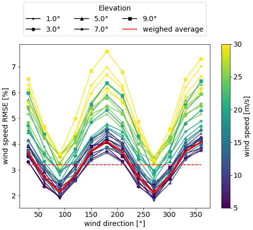
Figure A1 RMSE of simulated VAD. The resulting RMSE is calculated for 100 runs of each combination of parameters as shown in Table A2. Lines in red represent values weighed with the frequency distribution of wind speed and wind direction at the site. The dashed line represents the average of the continuous red line.

Lundquist et al. (2015)

Table A1 Summary of uncertainty components that contribute to the global uncertainty of the wind measurement with the scanning lidar and analysis techniques used during this project.

Table A2 Parameter set-up for the VAD simulation.

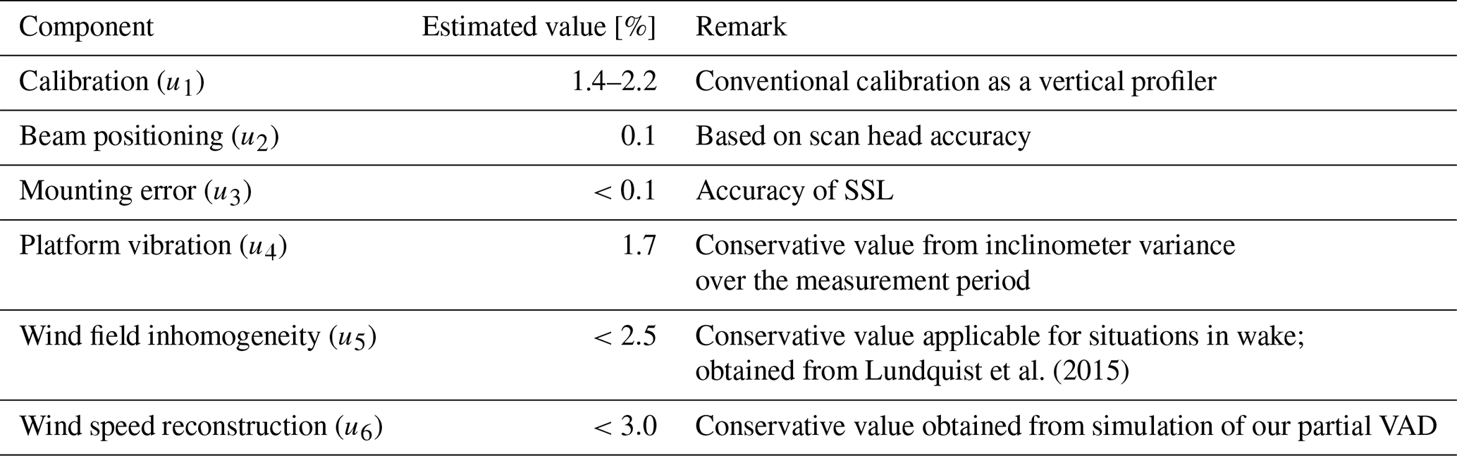
A1 Calibration

Prior to offshore deployment of the lidar, a calibration of the system was performed using a reference measurement. For this campaign, the calibration of the system was performed according to the calibration procedure for conventional vertical profilers (IEC-61400-12-1, 2017) at UL's test field in Wehlens in northern Germany. This means that we reproduced the measurement performed by a short-range vertical profiler with an elevation angle of 60^∘. The uncertainties obtained in this way are assumed to be conservative if compared to a line-of-sight calibration, as suggested by Borraccino et al. (2016). This increased uncertainty is due to the large height span and associated wind shear within a single range gate. During the campaign, the maximum elevation angle was closer to 7^∘, and hence the height range covered by a single range gate is significantly smaller. Accordingly, the actual uncertainty is expected to be smaller than that obtained during the system verification.

A2 Beam positioning

Another uncertainty component is the lidar laser beam positioning, which describes the combined effect of the accuracy of the scanning head in the vertical direction and the vertical wind shear. Here we used scanning lidar precision as given by the manufacturer and used a vertical power-law profile with an exponent α=0.14.

The error of the measurement height due to the curvature of the Earth is considered negligible at the range distance of the measurement location (1.5 km).

A3 Mounting error

The mounting error has been quantified by means of SSL. This has been taken into account in the scanning trajectory design to compensate for it. In this way we almost diminish this error; however there is still a very small remaining error.

A4 Platform vibration

Height variations in the measurement are caused by orientation changes in tilt and roll, due to platform vibration. An analysis of these signals from the internal inclinometer has been performed over the whole campaign. Finally, the effect of wind shear has been evaluated based on an assumption of a power-law profile with an exponent of α=0.14.

A5 Wind field inhomogeneity

The effect of inhomogeneous flow, mainly caused by partial wake effects, has been evaluated based on simulation results from Lundquist et al. (2015). The value is based on the assumption of a wake distance of nine rotor diameters downstream.

A6 Wind speed reconstruction

Additionally, as pointed out in Newsom et al. (2017) with respect to the VAD method, deviations from the perfect sinusoidal occur due to spatial and temporal fluctuations in the velocity field and instrumental errors, and in the context of the VAD algorithm, any departure from the perfect sinusoidal may be regarded as error. Due the lack of a proper physical set-up during this study, numerical simulations have been performed to assess the robustness of the calculation chain of the partial VAD. The results show an average of approximately 3 % mean error due to wind field inhomogeneity on our partial VAD procedure. This can be seen as a conservative estimation of uncertainty in the wind field reconstruction.

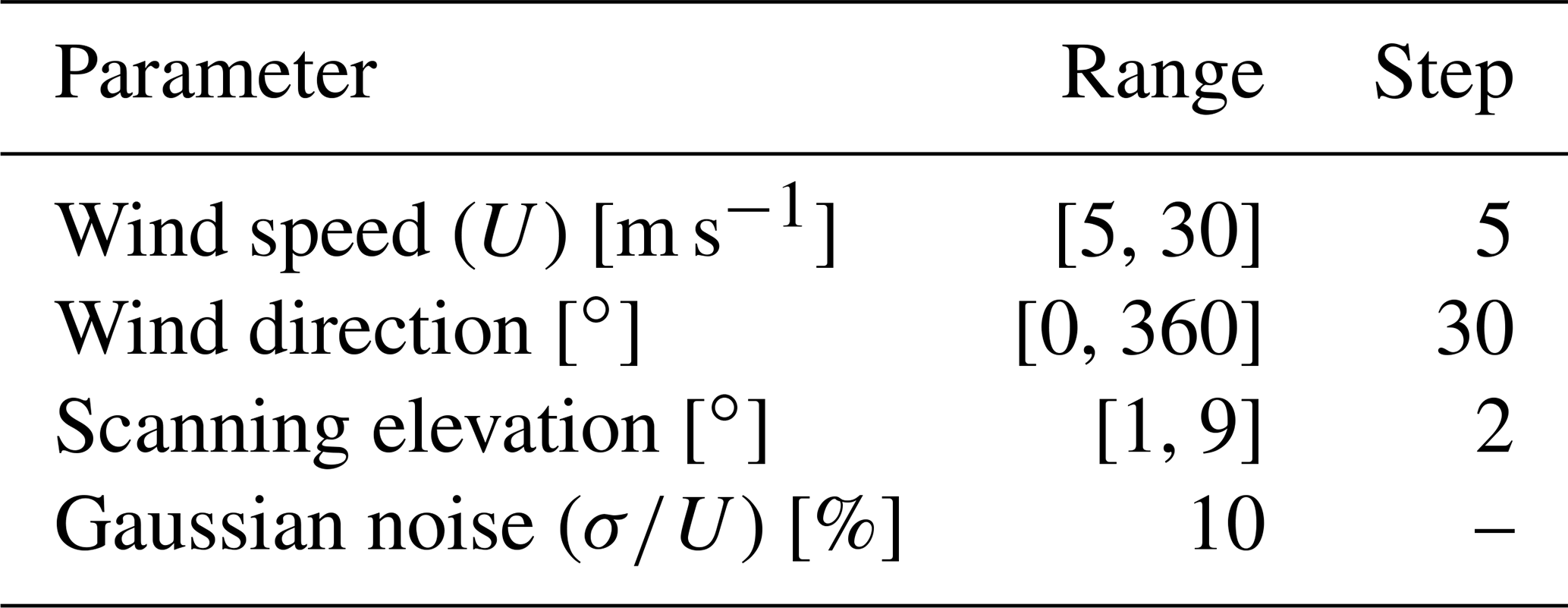
The simulations were based on synthetic fields with a defined mean wind speed (U) with superimposed Gaussian random noise $\mathit{\sigma }/U=\mathrm{10}\mathit{\%}$. The wind field was scanned with the same geometry as our partial VAD and for all combinations of parameters shown in Table A2.

The results in Fig. A1 show the root-mean-square error (RMSE) of simulations against the reference mean wind speed for 100 runs of each parameter combination. A dependence of the wind field reconstruction on both the azimuth opening angle of the scan trajectory and the wind speed can be observed. An average value was obtained based on the dependencies and wind speed distribution.

Six sources of uncertainty have been identified that play a role in the overall uncertainty of the lidar wind speed. Assuming that these uncertainties are independent, they can be combined in quadrature to yield

$$\begin{array}{}\text{(A1)}& u_{\mathrm{lidar}}^{\mathrm{2}}=u_{\mathrm{1}}^{\mathrm{2}}+u_{\mathrm{2}}^{\mathrm{2}}+u_{\mathrm{3}}^{\mathrm{2}}+u_{\mathrm{4}}^{\mathrm{2}}+u_{\mathrm{5}}^{\mathrm{2}}+u_{\mathrm{6}}^{\mathrm{2}},\end{array}$$

and therefore the overall lidar uncertainty in wind speed ranges between 4.4 % and 4.8 %, which is largely dominated by the wind field inhomogeneity and wind speed reconstruction. It is worth noting that these values are very conservative and are expected to be lower in the case of the wind-free sectors.

Appendix B: Weibull probability density function of wind speed scanning lidar per wind sector area

Figure B1 is an extension of Fig. 10 in the main text that shows the probability density function of wind speed scanning lidar per wind sector area using the largest free-wind sector (related to region R5) as reference. The bars shown have a width of 1 m s⁻¹. The height of the bars corresponds to the normalized density function, i.e., the frequency of the measured values contained in a bar multiplied by the bar width.

Figure B1 Weibull probability density function (pdf) of wind speed scanning lidar per wind sector area. The sector R5 is used as a reference.