the Creative Commons Attribution 4.0 License.
the Creative Commons Attribution 4.0 License.
 | 19 Jul 2022
The wide range of factors contributing to wind resource assessment accuracy in complex terrain
Alain Schubiger
Sara Koller
Dominik Eggli
Alexander Radi
Andreas Rumpf
Hermann Knaus
Understanding the uncertainties of wind resource assessments (WRAs) is key to reducing project risks, and this is particularly challenging in mountainous terrain. In the academic literature, many complex flow sites have been investigated, but they all focus on comparing wind speeds from selected wind directions and do not focus on the overall annual energy production (AEP). In this work, the importance of converting wind speed errors into AEP errors when evaluating wind energy projects is highlighted by comparing the results of seven different WRA workflows at five complex terrain sites. Although a systematic study involving the investigation of all possible varying parameters is not within the scope of this study, the results allow some of the different factors that could lead to this discrepancy being identified. The wind speed errors are assessed by comparing simulation results to wind speed measurements at validation locations. This is then extended to AEP estimations (without wake effects), showing that wind profile prediction accuracy does not translate directly or linearly to AEP accuracy. This is due to the specific conditions at the site, to differences in workflow set-ups between the sites and to differences in workflow AEP calculation methods. The results demonstrate the complexity of the combined factors contributing to WRA errors – even without including wake effects and other losses. This means that the wind model that produces the most accurate wind predictions for a certain wind direction over a certain time period does not always result in the most suitable model for the AEP estimation of a given complex terrain site. In fact, the large number of steps within the WRA process often lead to the choice of wind model being less important for the overall WRA accuracy than would be suggested by only looking at wind speeds. It is therefore concluded that it is vitally important for researchers to consider overall AEP – and all the steps towards calculating it – when evaluating simulation accuracies of flow over complex terrain. Future work will involve a systematic study of all the factors that could contribute to this effect.
- Article
(5428 KB) - Full-text XML
- BibTeX
- EndNote


Understanding the uncertainties of wind resource assessments (WRAs) is key to reducing project risks. This is particularly challenging in mountainous terrain, e.g. Bowen and Mortensen (1996), Wood (1995) and Pozo et al. (2017), which accounts for around 30 % of the world's land surface (Sayre et al., 2018).
Several previous studies examine and compare the performance uncertainties of different wind modelling tools at mountainous or complex sites, including the Bolund hill blind test (Bechmann et al., 2011; Berg et al., 2011), the Askervain hill blind test (Bao et al., 2018) and the Perdigão field test (Menke et al., 2019; Barber et al., 2020a). However, they are all limited to comparisons of wind speeds for chosen wind directions or to time periods that are much shorter than those required for WRA.
In order to transform wind speeds into annual energy production (AEP), which is required for WRAs, the expected wind speeds at a planned wind turbine location need to be described in the form of a frequency distribution. If the planned wind turbine hub height differs from the height for which the wind speeds are available, a vertical extrapolation is required. The frequency distribution needs to be obtained for different wind direction sectors, because the wind flow at complex sites varies with direction. As well as this, the frequency distributions need to be extrapolated for the expected lifetime of the wind turbine (usually 20 years). The resulting frequency distributions then need to be converted to power using the expected power curve of the planned wind turbine. The expected powers then need to be multiplied by time, added up and scaled for a 1-year time period to estimate the AEP. If wake effects are expected, i.e. if the wind turbine is located within a wind farm, they need to be estimated using a wake model such as the Jensen model (Jensen, 1983), the Park model (Mortensen et al., 1998), the Larsen model (Larsen, 1988) and the dynamic wake meandering (DWM) model (Larsen et al., 2008). Other losses such as electrical losses, grid losses, curtailment losses, and shutdowns due to maintenance and any environmental restrictions due to bats, birds, noise, flicker, etc., are also estimated. Due to the large number of separate steps, data types and organisations involved in WRAs, it is challenging to accurately and robustly evaluate the accuracy of different tools or workflows for the entire process. A key obstacle is the lack of availability and suitability of relevant validation data.
The only previous studies examining the steps required for full WRAs are the set of CREYAP exercises (Mortensen et al., 2015) and a US-based study on annual energy production (AEP) errors (Lee and Fields, 2021). CREYAP stands for Comparison of Resource and Energy Yield Assessment Procedures and is carried out by Ørsted and the Technical University of Denmark. In the 2021 version, participants estimate the net energy yield for the Walney Extension wind farm, accounting for wind speed variations over time and across the site, as well as for turbine interaction losses (https://windeurope.org/tech2021/creyap-2021/, last access: 18 July 2022). A summary of the findings from the previous exercises concludes that most of the steps involved in WRA require significant improvement, and the study needs extending for complex terrain effects (Mortensen et al., 2015). The US-based study presents a very valuable literature review of the energy yield assessment errors across the global wind energy industry and provides a summary of how the wind energy industry has been quantifying and reducing prediction errors, energy losses and production uncertainties (Lee and Fields, 2021). In their work, a long-term trend indicating a reduction in the over-prediction bias was identified. Both of these studies provide valuable information; however, they are limited due to confidentiality issues connected with collecting data from the industry.
The goal of this work is therefore to examine and compare the accuracies of a range of simulations at different complex flow sites in terms of both wind speed and AEP. In order to achieve this, simulations with seven different wind modelling workflows at five different complex terrain sites were carried out, and the resulting wind speeds were compared to measurements at a validation location. This was then extended to AEP estimations (without wake effects), and the differences were examined. The workflows involved a range of wind modelling tools as well as a range of model set-ups and AEP calculation methodologies.
The paper is organised as follows: the methods applied in this work are described in Sect. 2, the results in terms of wind speed are presented in Sect. 3, the results are extended to AEP in Sect. 4 and the conclusions are discussed in Sect. 5.
2.1 The applied workflows
In this paper, the simulation set-ups are referred to as “workflows” to highlight the fact that each AEP estimation contains an entire workflow, i.e. many steps as well as the wind modelling part. For each workflow, the digital topography and surface roughness data for each site were downloaded from the satellite observation Copernicus database (https://land.copernicus.eu/, last access: 18 July 2022).
This work was part of a larger study developing a new decision process for selecting the WRA workflow that would expect to deliver the best compromise between skill and costs for a given wind energy project that is developed, with a focus on complex terrain (Barber et al., 2022). For this study, a large range of different wind models and WRA set-ups were chosen in order to understand the relationship between skill and costs. This means that for the present paper, a systematic study investigating the effect of different factors on the AEP errors could not be carried out. This is the topic of future work.
2.1.1 Underlying wind models
The workflows applied were associated with different wind models as follows.
-
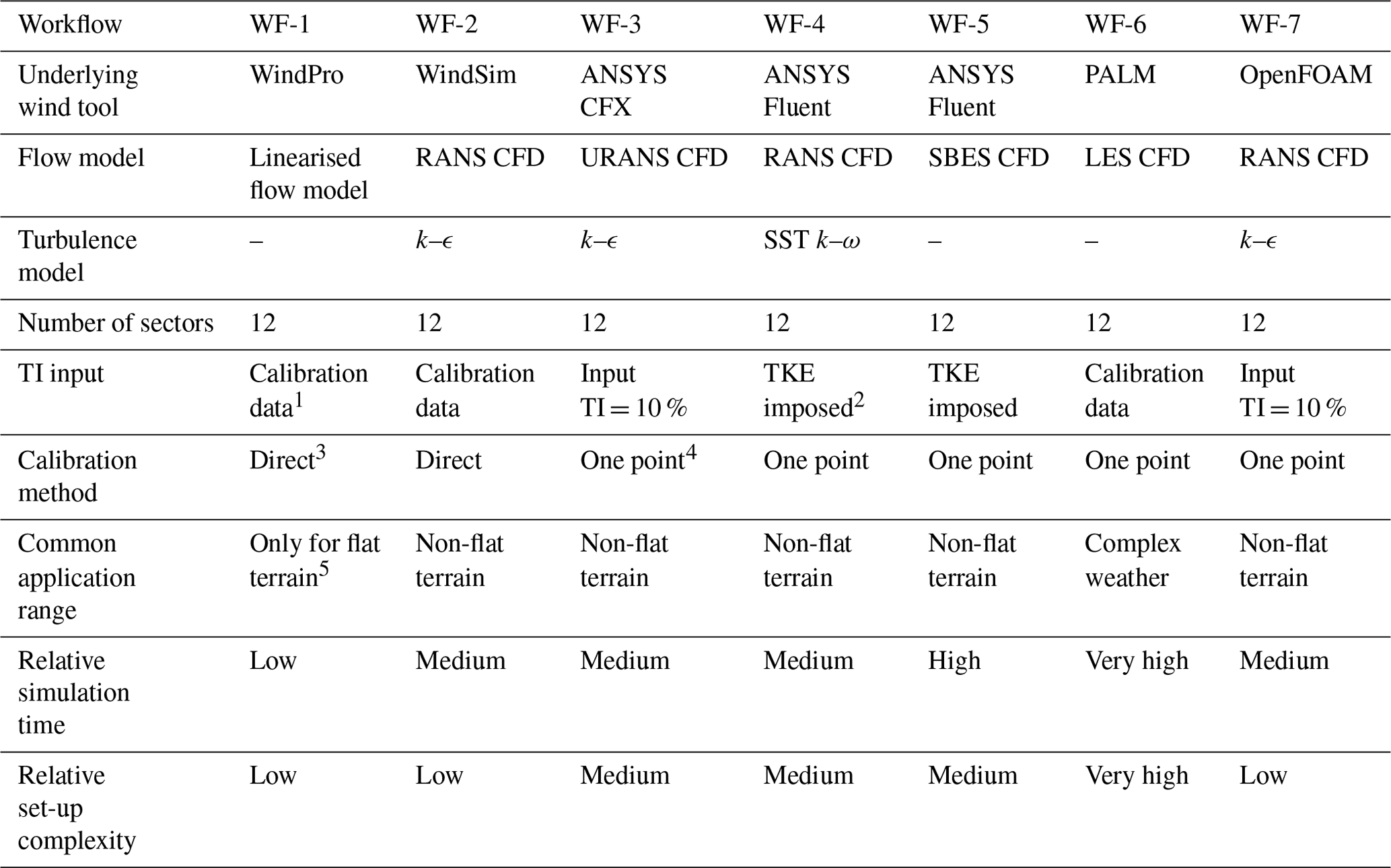
WF-1: WindPro. This is the industry-leading software suite for design and planning of wind farm projects (https://www.wasp.dk/, last access: 18 July 2022). It allows calibration data to be entered directly at the mast location and splits the flow into a total of 12 wind direction sectors. The turbulence intensity is calculated directly from the input met mast data standard deviations and mean values. In this work, the linearised flow model was applied, and no RIX (ruggedness index) corrections were applied.
-
WF-2: WindSim. This is an industry software using a computational fluid dynamics (CFD) model based on the PHOENICS code, a 3D Reynolds-averaged Navier–Stokes (RANS) solver from the company CHAM. It allows calibration data to be entered directly at the mast location and splits the flow into pre-defined wind direction sectors. The turbulence intensity is calculated directly from the input met mast data standard deviations and mean values. In this work, the simulations were conducted using the standard k–ϵ turbulence model (Rodi and Spalding, 1983). The boundary condition at the top was fixed pressure. A total of 12 wind direction sectors were used.
-
WF-3: ANSYS CFX. This is an all-purpose CFD software. In this work, ANSYS CFX (version 19.2) was applied using an unsteady RANS (URANS) approach in combination with the standard k–ϵ model (Rodi and Spalding, 1983). The equation system was extended to an anelastic formulation whereby the density is influenced by buoyancy forces using the Boussinesq approximation (Montavon, 1998). The Earth's rotation was considered with additional terms in the momentum equation to describe the Coriolis force at a given angular velocity. Forested areas were considered through a canopy model (Liu et al., 1996). Individual roughness lengths of the canopy were attributed to each land use and are chosen according to the work of Wiernga (Wiernga, 1993). These methods have previously been applied successfully to other applications (Knaus et al., 2017). Static boundary conditions were applied around the resolved volume for the chosen wind direction and wind speed, forming a Taylor spiral. Since the upper boundary condition of the domain is flat but the ground surface is not, the mass flow rate was balanced at the top surface of the domain in order to prevent an acceleration due to mass conservation of the set-up. Turbulence was introduced by entering a turbulence intensity of 10 % as an input condition. In order to match the WindPro and WindSim simulations, a total of 12 wind direction sectors were simulated. This was implemented by developing a new simulation workflow using a Python script as described in Barber et al. (2020b).
-
WF-4: Fluent RANS. ANSYS Fluent is a commercial CFD tool for modelling the flow in industrial applications and can be set up to solve the RANS equations, as well as for the large eddy simulation (LES) or detached eddy simulation (DES) approach. In this work, Fluent was first set up to solve the RANS equations with the SST k–ω turbulence model (Menter, 2012). The inlet wind speed profiles, turbulent kinetic energy and turbulent dissipation rate were imposed based on the roughness height according to Richards and Hoxey (1993). In order to match the WindPro and WindSim simulations, a total of 12 wind direction sectors were simulated. This was implemented by developing a new simulation workflow using a Python script as described in Barber et al. (2020b).
-
WF-5: Fluent SBES. A technique within ANSYS Fluent called stress-blended eddy simulation (SBES) was applied. SBES is a new model that offers improved shielding of RANS boundary layers and a more rapid RANS–LES transition, amongst other things. The RANS results were used to initialise SBES, which was performed unsteadily with an adaptive time stepping procedure ensuring a Courant–Friedrichs-Lewy number (CFL) ≤ 1. After an additional unsteady initialisation, the wind speeds were averaged over 10 min. The wind rose measured at the met mast was used to choose the main wind directions, and only these directions were simulated. In order to introduce fluctuating velocities at the inlet, the Fluent synthetic turbulence generator was used. In order to save computational power, all 12 wind direction sectors were not simulated. Instead, only the most frequently occurring sectors were simulated, and Fluent RANS results were used for the other sectors. In this work, two separate workflows were applied – for workflow WF-5a, three sectors were simulated with SBES, and for workflow WF-5b, seven sectors were simulated with SBES. This was implemented by developing a new simulation workflow using a Python script as described in Barber et al. (2020b).
-
WF-6: PALM. The model PALM is based on the non-hydrostatic, filtered, incompressible Navier–Stokes equations in Boussinesq-approximated form (an anelastic approximation is available as an option for simulating deep convection). Furthermore, an additional equation is solved for the subgrid-scale turbulent kinetic energy using large eddy simulations (LESs) (https://palm.muk.uni-hannover.de/trac/wiki/palm, last access: 18 July 2022). In this work, due to the long computational time, not all sectors could be simulated. Instead, the most frequent sectors were simulated and complemented with the WindSim simulations. The TKE-1 turbulence model was applied.
-
WF-7: E-Wind. E-Wind solves the 3D RANS equations, with a modified kk–ϵ turbulence closure. The governing equations are implemented in the open-source toolbox OpenFOAM (Alletto et al., 2018). It is based on a steady-state two-equation RANS model and includes the effect of forests, Coriolis force, and buoyancy in the turbulence equations. It has only been applied to Site 3 in this work, due to the interest of the E-Wind developers, Enercon, in that site.
Table 1Summary of the long-term extrapolation methods for each site.

* MCP: measure–correlate–predict method.
2.1.2 Simulation calibration
For each site, measurement data were available for at least two different locations, and the most available and reliable data at the location closest to the planned or existing wind turbine hub height(s) was chosen for calibration. For WindPro and WindSim, the calibration data could be directly input into the tool. For the CFD simulations, the calibration was undertaken for each wind direction sector simulated by inputting a generic logarithmic wind profile calculated using the roughness height value at the simulation input location (Richards and Hoxey, 1993). Then, the simulation results were scaled by a constant calibration factor, defined as the ratio between the simulated and the long-term-corrected measured wind speed at the calibration location.
2.1.3 Simulation validation
For each site, the second measurement point was taken for the validation. The validation was carried out by first calculating the wind speed and direction at the validation location for each calibrated wind direction sector simulation and then by comparing these values to the measurements.
2.1.4 Wind speed long-term extrapolation
For each site, the long-term-corrected measured wind speed was obtained at both the calibration and validation locations by firstly averaging the wind speeds over a time period for which valid data were available for both the calibration and validation measurements. Secondly, these average wind speeds were extrapolated for a 20-year period using the measure–correlate–predict method with long-term reference data. These data were obtained either from a nearby met mast or from MERRA-2 data (https://gmao.gsfc.nasa.gov/reanalysis/MERRA-2/, last access: 18 July 2022), as summarised in Table 1.
2.1.5 AEP calculation
The wind industry tools applied in this work, WindPro and WindSim, as well as E-Wind, offer a user interface containing all the steps required to get from wind measurements to AEP predictions. However, the other CFD tools, Fluent, CFX and PALM needed to be extended in order to calculate the AEP. In previous work (Barber et al., 2020b), automated workflows for carrying out wind flow modelling in complex terrain were developed for the commercial CFD tools ANSYS Fluent and ANSYS CFX. These processes included a pre-processing tool, a meshing script, a simulation script and a pre-processing tool. It was shown that the total simulation costs, including model set-up and post-processing effort costs, could be reduced by a factor of 12 for Fluent and seven for CFX through this automation. For PALM, a slightly different method was applied in order to reduce the computational time in a pragmatic way. This involved firstly searching for a time period in the met mast data for which the wind speed remained relatively stable at the average wind speed for each wind direction sector. For this time period, COSMO-D2 data (http://www.cosmo-model.org/content/tasks/operational/dwd/default_d2.htm, last access: 18 July 2022) were taken for the PALM boundary conditions by reading the data from a dynamic input file (offline nesting). Finally, this time period is simulated with PALM, and the average wind speed is extracted for the calibration and validation positions at the reference height.
Table 2Summary of AEP comparisons for the different methods used in this paper.
In the present work, these workflows were extended to include AEP estimations. The AEP was calculated at the validation location(s) as follows.
-
Speed-up factors between the validation location(s) and the calibration location were calculated from the simulation results for each wind direction sector (in this case, 12 sectors). The speed-up factor is defined as the ratio between the wind speed at the validation location to the wind speed at the calibration location.
-
Option “Time series method”:
-
The amount of wind turning between the validation location(s) and the calibration location was calculated from the simulation results for each wind direction sector.
-
Based on the wind direction sector, each measured 10 min averaged wind speed at the calibration location was multiplied by the relevant speed-up factor to obtain the expected wind speed at the validation location for that 10 min period.
-
For sectors with a wind direction turning larger than ±15∘, each data point was moved to the relevant new sector.
-
The linearly interpolated bin-averaged power curve provided by the manufacturer with 1 m s−1 wide bins was used to obtain the expected power production for every 10 min wind speed at the validation location(s). For this, it was assumed that the wind speed at the validation location remained constant over the entire wind turbine rotor area. The rotor equivalent wind speed was not used because the commercial tools do not use this method and a fair comparison was required.
-
These powers were each multiplied by 10 min and added up to obtain the total energy production over the measurement period.
-
-
Option “Weibull method”:
-
A frequency distribution of the calibration location data was created for each sector.
-
A Weibull distribution was fitted to each frequency distribution.
-
The Weibull distributions were scaled for each sector using the simulated speed-up factors. The shape factor was kept constant.
-
The scaled Weibull distributions were multiplied by the bin-averaged power curve provided by the manufacturer with 1 m s−1 wide bins to obtain the total energy production over the measurement period.
-
-
The total energy production was converted to AEP by scaling the energy production in each wind direction sector linearly with the total measurement time.
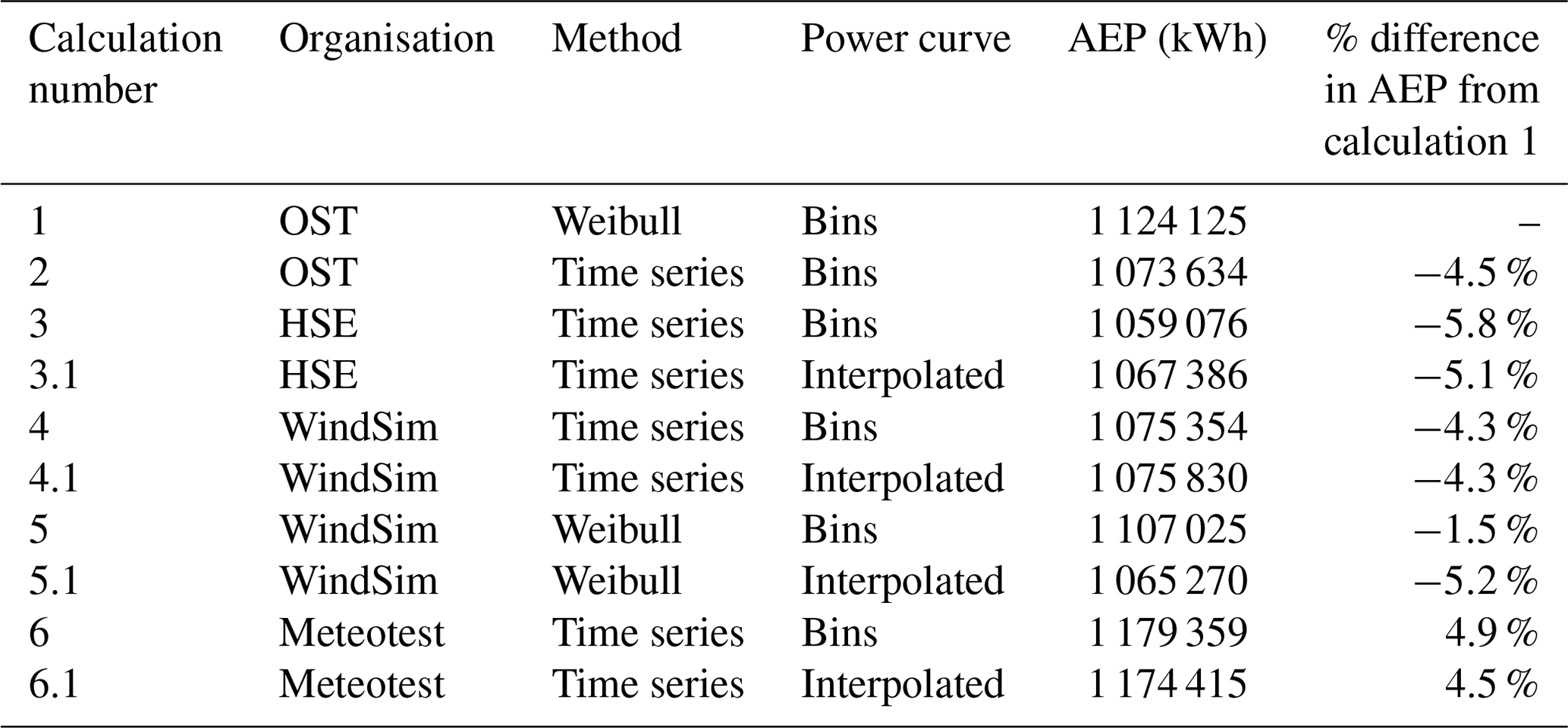
The three research partners in this project, OST (Eastern Switzerland University of Applied Sciences), HSE (Esslingen University of Applied Sciences) and Meteotest, created their own separate workflows for this AEP calculation. For validation purposes, the workflows were firstly compared to each by entering the same simulation results from the WindSim model at one site (Site 1; see description in Sect. 2.2). An overview of the results is shown in Table 2. As well as comparing the results between organisations, the time series method and the Weibull method are compared. Finally, the effect of interpolating the power curve or simply using the 1 m s−1 wide bins is compared.
As can be seen in the right-hand column, which shows the percentage difference in AEP for each calculation compared to calculation number 1, the variation in AEP between the different partners is less than 5 %, giving us a general confidence in the methods. The largest variation is between the Weibull method and the time series method (3.4 % for the OST method). The difference between the power curve bins and the interpolation is small (1.2 % for the OST method, 0.6 % for the HSE method and 0.1 % for the WindSim method). It should be noted that 5 % is not an insignificant amount of energy, and the variations between methods are surprising to the authors. A significant effort in comparing the methods and correcting small errors did not lead to a reduction in these differences.
Table 3Summary of the seven workflows used in this study.
1 Calculated directly from calibration data using mean and standard deviation of wind speed. 2 Turbulent kinetic energy and turbulent dissipation rate imposed based on roughness height at input location from roughness map. 3 Calibration data entered directly. 4 One-point calibration of generic log profile using roughness height. 5 Usually defined as slopes below 30 % (Bowen and Mortensen, 1996).
2.1.6 Summary of workflows
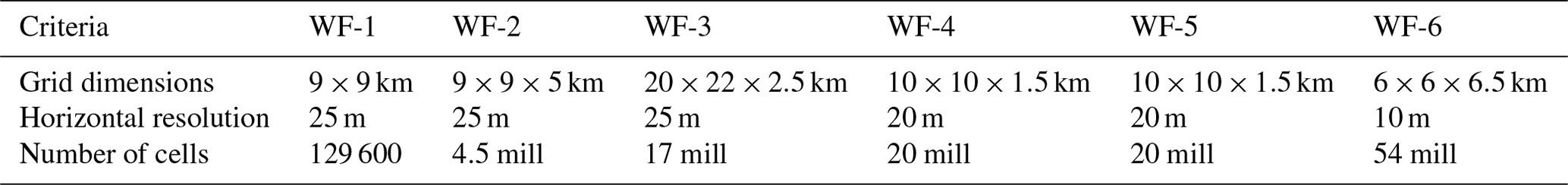
The different set-ups for each workflow are summarised in Table 3. As well as describing the underlying wind tool, the flow model, the turbulence model, the number of wind directions simulated, the turbulence intensity (TI) input method and the calibration method applied, the last three rows compare the common application range of the tools as well as their relative simulation time and relative set-up complexity, in order to give the reader a feel for the type of workflows applied. The relative simulation time and set-up complexity are key factors when choosing the most optimal workflow for a given application. This topic has been studied in detail in a separate paper by the same authors (Barber et al., 2022).
2.2 The simulated sites
An overview of the simulated sites is shown in Fig. 1 and in Table 9, except for Site 5, which is confidential. The details and the workflow set-ups for each site are described in the individual sections below.
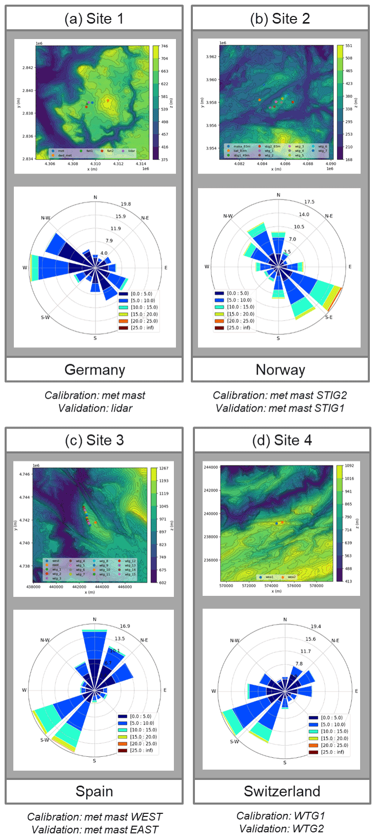
Figure 1An overview of four of the five sites simulated in this work (Site 5 is confidential): (a) Site 1, (b) Site 2, (c) Site 3 and (d) Site 4.
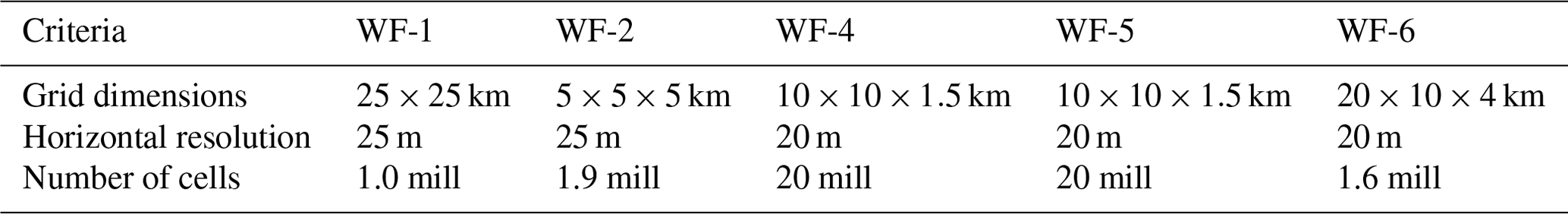
Table 4Set-up of the workflows at Site 1. “mill” stands for millions.
2.2.1 Site 1
Site 1 is a complex terrain, partly forested site close to Stötten in southern Germany, whose central feature is a steep incline above 30 % and a main wind direction of W. Wind speed and direction data were available from a met mast located about 1 km away from the incline, as well as a lidar, as described in Schulz et al. (2014). In this paper, the met mast data from four cup anemometers with an accuracy of 1 % and three 3D sonic anemometers with an accuracy of 1.5 % were used for calibration, and the wind speed data recorded using the SWE (Stuttgarter Lehrstuhl für Windenergie) scanner, a fast pulsed lidar wind scanner based on a Leosphere WindCube V1 system with an adapted scanner unit, were used for validation. The coordinates of the calibration location are (4309721.715, 2838928.447) (coordinate system EPSG3035). For the measurement campaign used in this work, the lidar was positioned approximately 300 m west of the met mast for approximately 1 year (March 2015–February 2016). An overview of the site and the wind rose from the met mast at 98 m over the entire measurement period are shown in Fig. 1. S & G Engineering SG750.54 wind turbines with a hub height of 100 m are planned at the site. The details of the applied workflows are shown in Table 4. WF-7 was not applied to this site.
2.2.2 Site 2
Site 2 is an existing wind farm site in Norway surrounded by a terrain of hills, lakes and forests. The wind farm consists of seven Siemens SWT-DD-130 wind turbines with a hub height of 115 m located on a small hill as shown on Fig. 1. The circles on this figure refer to met masts and wind turbines. Another wind farm consisting of 22 wind turbines is located on the hill to the north of the wind farm. The two main wind directions are SE and NW, as can be seen on the wind rose from the met mast STIG2 in Fig. 1. In this project, the two met masts close to the wind turbines, STIG1 and STIG2, are used. For STIG1, wind speed measurement data are available from Thies First Class cup anemometers at five heights up to 50 m from June 2007 to May 2016 (9 years). For STIG2, wind speed measurement data from cup anemometers are available at five heights up to 83 m from December 2013 to January 2016 (2 years). STIG1 has three sensors at very similar heights (48, 49 and 50 m), whereas STIG2 has two sensors at similar heights (82 and 83 m). An examination of the time series of the measurement data showed that the sensors at 47, 48 and 82 m contained some errors, and therefore the sensors at these heights were not used. STIG2 at 83 m is taken as the calibration mast, with coordinates of (4086674.443, 3958009.528) (coordinate system EPSG3035). The details of the applied workflows are shown in Table 5. WF-3 and WF-7 were not applied to this site.
2.2.3 Site 3
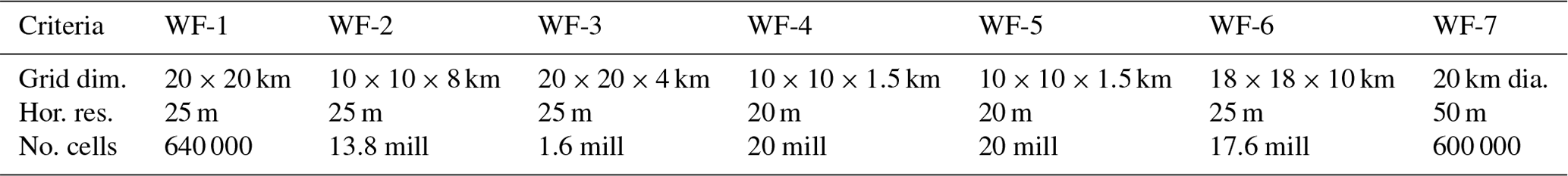
Site 3 is an existing wind farm site in Spain situated in complex terrain. The wind farm consists of 15 Enercon E-40 wind turbines with a hub height of 50 m located at the top of a steep ridge as shown in Fig. 1. The circles on this figure refer to met masts and wind turbines. The two main wind directions are SW and SWW, as can be seen on the wind rose in Fig. 1. In this project, data from two met masts, “east” and “west”, were used. For both of these masts, measurement data were provided from Thies First Class cup anemometers at a range of heights up to 50 m from September 2009 to September 2010. Due to the high amount of overlapping data points (48 941), they can be used for the calibration and validation data reliably. The west mast was used for calibration and the east mast for validation. The coordinates of the calibration location are (442929.200, 4741536.600) (coordinate system EPSG3035). The details of the applied workflows are shown in Table 6. All seven workflows were applied to this site.

2.2.4 Site 4
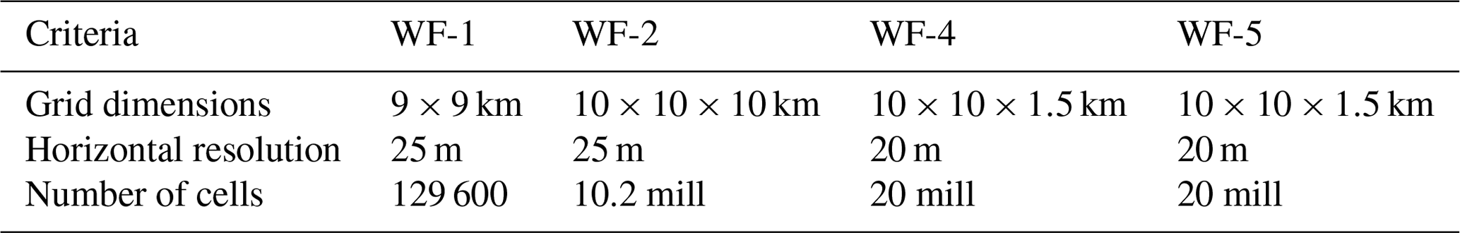
Site 4 is the existing St. Brais wind farm site in Switzerland situated in complex terrain. The wind farm consists of two Enercon E-82 wind turbines with a hub height of 78 m located as shown in Fig. 1. The main wind direction is SW, as can be seen on the wind rose on the figure. In this project, wind speed and direction data from the two wind turbines WEA1 and WEA2 were used, because no met mast data were available. The measurement location on the nacelle of the wind turbines (hub height 78 m) means that the data will be influenced by the wind turbine rotors, and the measurements will not correspond to the freestream wind speed. It is not known if the measurement data include any kind of correction for this effect or not. This means that the data needs to be used carefully in this project, and the results will only be able to be used indicatively. This is discussed further in Sect. 4. The absolute values of the wind speeds may not be correct, but the ratios will still be valid, assuming that there are no large discrepancies in the operation of the wind turbines. For both of these wind turbines, measurement data were provided from January 2010 to December 2020, a time period of 10 years. Due to the high amount of overlapping data points (554 045), they can be used for the calibration and validation data reliably. A long-term extrapolation was not done because the measurement period is already very long. The wind turbine WEA1 was used for calibration and WEA2 for validation. The coordinates of the calibration location are (574452.000, 239147.000) (coordinate system EPSG21781). A good correlation between the WEA1 and WEA2 data could be seen. The details of the applied workflows are shown in Table 7. The workflows WF-3, WF-6 and WF-7 were not applied.
2.2.5 Site 5
Site 5 is a planned site that cannot be described in detail here for confidentiality reasons. However, the results are still included in this work in the form of comparisons. The site is located in hilly terrain. Data from two met masts over a time period of 6 months are available. The met mast closest to the planned wind turbines was chosen for the calibration point. The details of the applied workflows are shown in Table 8. The workflows WF-3, WF-6 and WF-7 were not applied.
For each site, a total of 12 simulations were carried out – one for each 30∘ wind direction sector. In this section, the simulation results are shown in terms of absolute differences between the measurements and simulations at the calibration and validation locations for each site. For locations with data at more than one height, the root mean square error of all measured heights compared to simulations is used as a comparison.
Detailed simulation results for each site can be found in the final project report (Barber et al., 2021). This includes speed-up factors and turning between calibration and validation locations, comparisons of simulated and measured wind speed, and direction profiles for all wind directions and wind speed contours.
3.1 Site 1
The average RMSE values between the simulations and the measurements over all 12 wind direction sectors are shown in Fig. 2. The top row (a and b) shows the calibration location and the bottom row (c and d) the validation location. The left-hand plots (a and c) show the results of a simple averaging of the RMSE values over the 12 wind direction sectors, whereas the right-hand plots (b and d) show RMSE averages weighted for the wind speed frequency distribution measured at the calibration location. This weighted averaging gives more weighting to more frequent wind speeds in an attempt to provide a number more relevant for the AEP. For this site, it can be seen that the weighted averaging does not have a large effect on the results. This indicates that the errors of the most frequent wind directions are close to the average value.

Figure 2Site 1 – RMSE values between the measurements and simulations at (a) the calibration location and (b) the validation location for different numbers of measurement heights, for simple and weighted wind direction sector averaging (m s−1).
The different bars in each plot represent different measurement heights that have been taken to calculate the RMSE, with the number of points increasing with increasing darkness of the colours. The light-green colour refers to just one point, and therefore the RMSE is equal to the absolute difference between measured and simulated wind speed. This number is very low for the calibration location as expected because of the calibration method described in Sect. 2.1,2. The measurement heights used for these calculations were 10, 25, 50, 75 and 100 m. However, the error is not exactly equal to zero because the grid point in the simulation mesh nearest to the calibration position was taken for the calibration. This had a slight deviation in both the horizontal and vertical direction.
For the calibration location, the variable “RMSE 25–100 m” refers to the RMSE value using all the measurement heights except for the lowest point, because this point is difficult to simulate accurately and also less relevant for the AEP calculation as it is not inside the rotor area of the planned wind turbines. “RMSE 10–100 m” refers to the RMSE value using all the measurement heights. The values increase with an increasing number of points, because the simulations become less accurate close to the ground. This is expected, especially for heights below 25 m. In general, the results at the calibration location indicate that the wind speed profile has not been captured well for all workflows, even if the lower points are removed.
For the validation location, the variable “RMSE 75–125 m” refers to the RMSE value using only the heights within the rotor area of the planned wind turbines, and “RMSE 50–150 m” refers to the RMSE value using all the measurement heights. The values increase with an increasing number of points, because the simulations become less accurate close to the ground. This is expected, especially for heights below 25 m. However, this effect is not as large as for the calibration location. In general, the entire profile is predicted fairly inaccurately, which is surprising due to the close location of the calibration and validation location (see Fig. 1). Another thing to notice about the RMSE values at the validation location is the particular low accuracy of WF-1 (WAsP) compared to the other workflows.
Examination of the absolute wind speed contours from the Fluent RANS simulations, shown in Fig. 7, indicate that the wind speeds are not expected to deviate significantly between the calibration and validation locations at any of the three main wind directions. The reasons for these validation errors of almost 1 m s−1 are not entirely clear and could be due to a measurement error. This is being further investigated.
3.2 Site 2
For Site 2, measurement data were only available at one height. Therefore, the average absolute differences between the measurements and simulations over all 12 wind direction sectors at (a) the calibration location and (b) the validation location at hub height are shown in Fig. 3. The different bar colours represent simple and weighted averaging of the wind direction sectors, as introduced in the previous section. The error at the calibration location is very small, remaining below 0.006 m s−1 for each workflow. For the validation location, the errors all remain below 1 m s−1. WF-1 (WindPro) and WF-2 (WindSim) are closer to the measurements than WF-5 (Fluent) and WF-6 (PALM). For these three workflows, the order of the validation errors are similar to Site 1. Examination of the absolute wind speed contours at a height of 100 m above the ground for the three most common wind directions calculated using Fluent RANS in Fig. 8 indicates that varying validation errors between workflows could be caused by varying capabilities of capturing the flow over the hill, especially in the 30∘ direction. This is discussed in more detail in the final project report (Barber et al., 2021). The weighted averaging affects both WF-1 (WindPro) and WF-2 (WindSim), but for WF-1 it increases the error and for WF-2 it decreases the error. The reason for this is not clear and is investigated in Sect. 4.
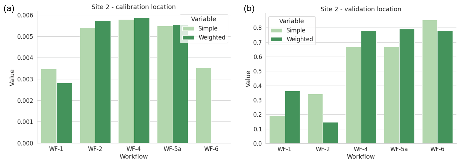
Figure 3Site 2 – absolute differences between the measurements and simulations at (a) the calibration location and (b) the validation location (m s−1).
3.3 Site 3
For Site 3, measurement data were only available at one height. Therefore, the average absolute differences between the measurements and simulations over all 12 wind direction sectors at (a) the calibration location and (b) the validation location are shown in Fig. 4. For the calibration location, the errors for all workflows are all below 0.08 m s−1. These errors are slightly larger than the other sites because the discrepancy between the actual calibration position and the nearest grid point is larger. For the validation location, the errors all remain between about 0.4 and 0.7 m −1, a similar range to Site 2. However, the difference between workflows is less significant. WF-4 (Fluent RANS) and WF-5 (Fluent SBES) are generally more accurate. The weighted averaging generally has a small influence on the results. For these three workflows, the order of the validation errors are similar to Site 1. Examination of the absolute wind speed contours at a height of 100 m above the ground for the three most common wind directions calculated using Fluent RANS in Fig. 9 indicates that varying validation errors between workflows could be caused by varying capabilities of capturing the flow over the hill, especially in the 30∘ direction. This is discussed in more detail in the final project report (Barber et al., 2021).
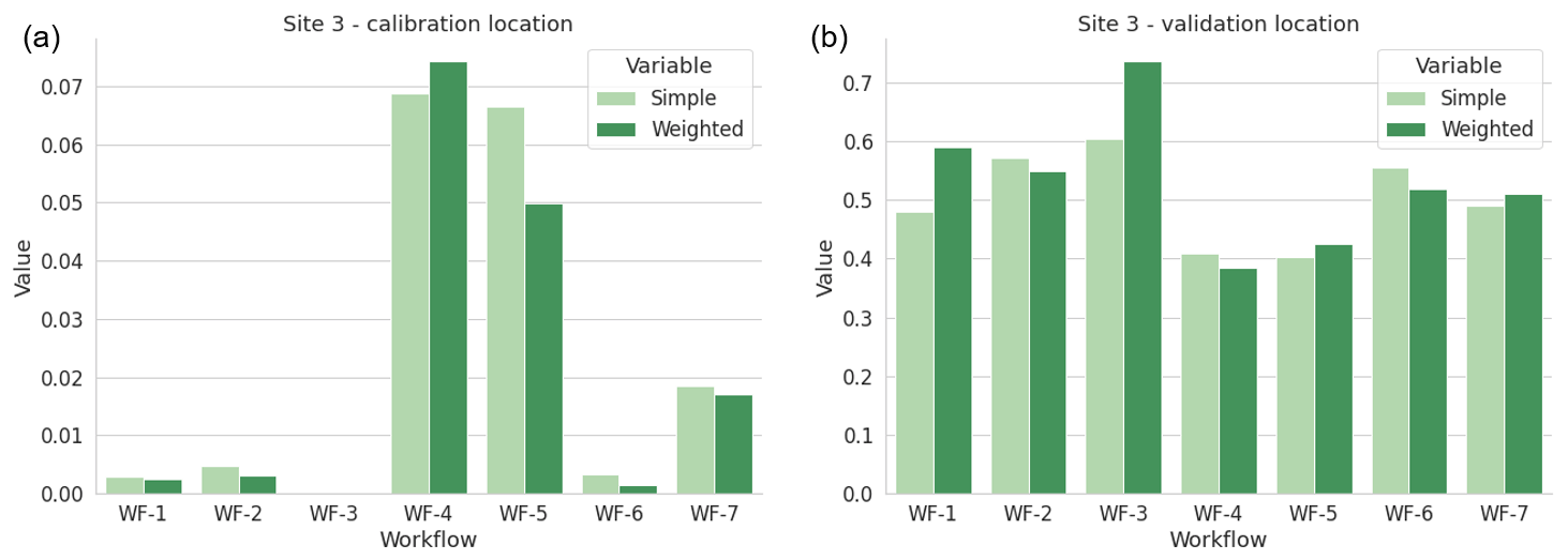
Figure 4Site 3 – absolute differences between the measurements and simulations at (a) the calibration location and (b) the validation location (m s−1).
3.4 Site 4
For Site 4, measurement data were only available at one height. Therefore, the average absolute differences between the measurements and simulations over all 12 wind direction sectors at (a) the calibration location and (b) the validation location are shown in Fig. 5. For the calibration location, the errors for all workflows are all below 0.06 m s−1, for the same reasons as described above. For the validation location, the errors are even lower than the previous sites, remaining below 0.5 m s−1. Similarly to Site 2, WF-1 (WindPro) and WF-2 (WindSim) are closer to the measurements than WF-4 (Fluent RANS) and WF-5 (Fluent SBES). Again, the weighted averaging generally has a small influence on the results. The absolute wind speed contours at a height of 100 m above the ground for the three most common wind directions calculated using Fluent RANS are shown in Fig. 10. Similarly to Site 1, the validation error is unexpectedly large considering the small distance and difference in height between the calibration and validations locations and perhaps reflects the poor quality of measurement data from the wind turbines compared to the met mast measurements at the other sites.
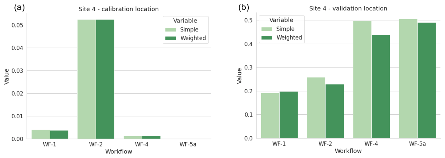
Figure 5Site 4 – absolute differences between the measurements and simulations at (a) the calibration location and (b) the validation location (m s−1).
3.5 Site 5
For Site 5, measurement data were only available at one height. Therefore, the average absolute differences between the measurements and simulations over all 12 wind direction sectors at (a) the calibration location and (b) the validation location are shown in Fig. 6. For the calibration location, the errors for all workflows are all below 0.02 m s−1, for the same reasons as described above. For the validation location, the errors are similar to Sites 1–3, remaining between 0.5 and 1 m s−1. The significant distance between the calibration and validation locations on two separate hills and the corresponding differences in flow modelling capabilities over these hills could cause these validation errors. The wind speed contours cannot be shown here due to confidentiality reasons. Similarly to Site 3, the difference between the workflows is not very large. However, the effect of the weighted averaging is not insignificant. This was found to be because the largest deviations from the measurements occurred at the more frequent wind speeds and is discussed further in Barber et al. (2021).
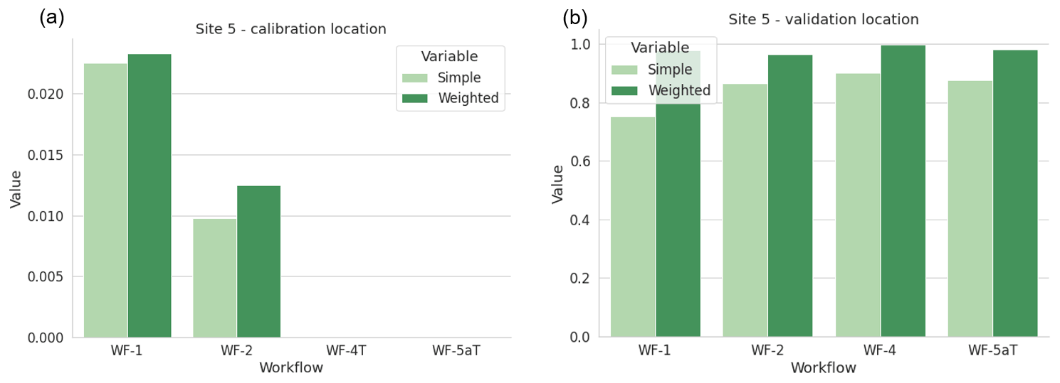
Figure 6Site 5 – absolute differences between the measurements and simulations at (a) the calibration location and (b) the validation location (m s−1).
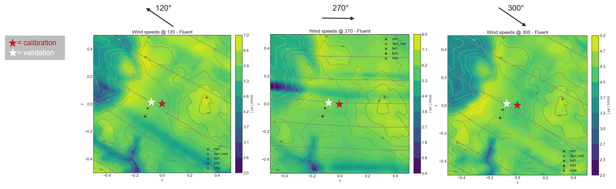
Figure 7Site 1 – absolute velocity contours for the three main wind directions simulated in Fluent RANS at 100 m a.g.l. (above ground level).

Figure 8Site 2 – absolute velocity contours for the three main wind directions simulated in Fluent RANS at 100 m a.g.l.
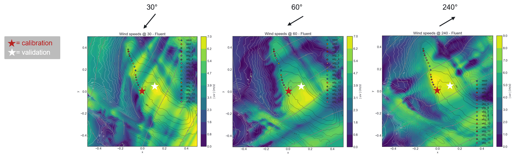
Figure 9Site 3 – absolute velocity contours for the three main wind directions simulated in Fluent RANS at 100 m a.g.l.
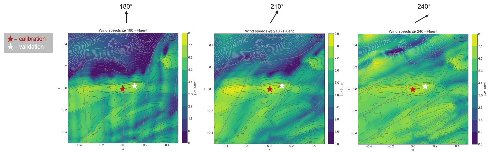
Figure 10Site 4 – absolute velocity contours for the three main wind directions simulated in Fluent RANS at 100 m a.g.l.
In this section, the results at the validation location for each site are shown in terms of AEP, which was calculated from the simulation results for each workflow as described in Sect. 2. There are no AEP measurements to compare the results with, so instead each result was compared to a theoretical value of AEP. This was determined using the AEP time series method described in Sect. 2.1.4, but instead of using the simulation results to scale the calibration data time series, the measured time series at the validation location was used directly. This allowed the effect of the simulated differences in wind speeds to be transferred to differences in AEP. Throughout this work, AEP refers to the gross production, i.e. without any losses or wake effects. Any workflow name with the letter “T” added to it indicated that flow turning effects were considered, as described in Sect. 2.1.5 – i.e. WF-3 refers to workflow WF-3 without turning considered and WF-3T with turning considered.
4.1 Site 1
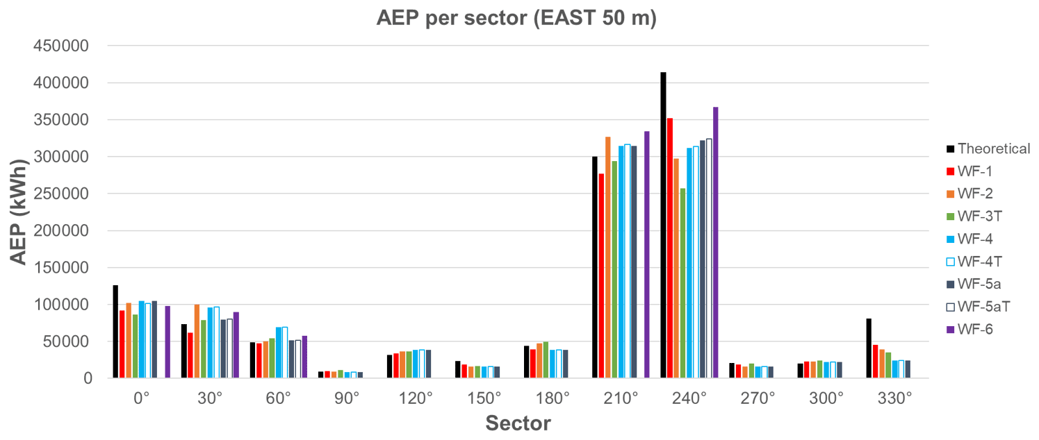
The wind turbine chosen for the AEP calculation at the validation location of Site 1 was a S & G Engineering SG750.54 with a hub height of 100 m, because this is the type planned for this site (construction planned in 2022). This wind turbine has a rated power of 750 kW and a rated wind speed of 11 m s−1. In order to calculate the AEP, each research partner implemented their own script according to the time series method described in Sect. 2.1.4. The results are shown in Fig. 11 in terms of the percentage differences from the theoretical value. All the results are significantly lower than the theoretical value. The differences in AEP are due to the differences in simulation results as well as the differences in the AEP methods between research partners. For WF-3 (CFX), a comparison was additionally made with and without the effects of turning (as described in Sect. 2.1.4). A very small difference due to the effects of flow turning was observed, shown by the difference between WF-3 and WF-3T. Details of the variations of the AEP for each wind direction sector can be found in the Appendix as well as in Barber et al. (2021). It was found that a large variation between model and sector exists, without a particular trend.
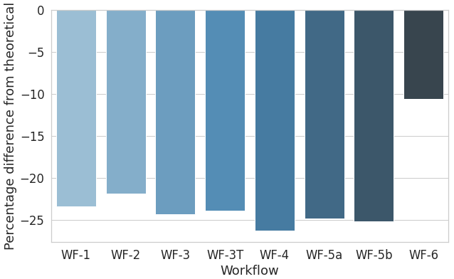
Figure 11Site 1 – percentage difference in gross AEP from the theoretical value for each workflow applied.
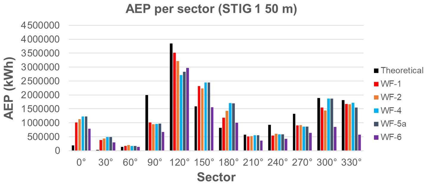
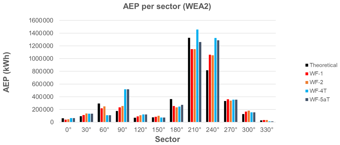
4.2 Site 2
For this site, the AEP has been calculated at the validation location using the power curve of the Siemens SWT-DD-130 wind turbine. A hub height of 50 m instead of the real hub height of 115 m was used in order to avoid additional inaccuracies due to the wind speed profile vertical extrapolation. This wind turbine has a rated power of 3.9 MW and a rated wind speed of 13 m s−1. The results in Fig. 12 show that the results match very well for WF-1 (WindPro), WF-2 (WindSim), WF-4 (Fluent RANS) and WF-5a (Fluent SBES), with deviations less than 3 %. The WF-6 (PALM) result is significantly lower, with a deviation of 32 %. This is due to the under-predicted wind speed shown in Sect. 3.
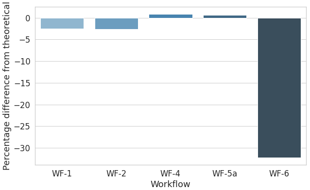
Figure 12Site 2 – percentage difference in gross AEP from the theoretical value for each workflow applied.
Details of the variations of the AEP for each wind direction sector can be found in the Appendix as well as in Barber et al. (2021). It was found that the AEP was under-predicted in the three most frequent sectors (120, 270 and 300∘), leading to an overall under-prediction of AEP. For WF-6 (PALM), the 270 and 300∘ sectors are especially strongly under-predicted, explaining the large deviation compared to the theoretical AEP.
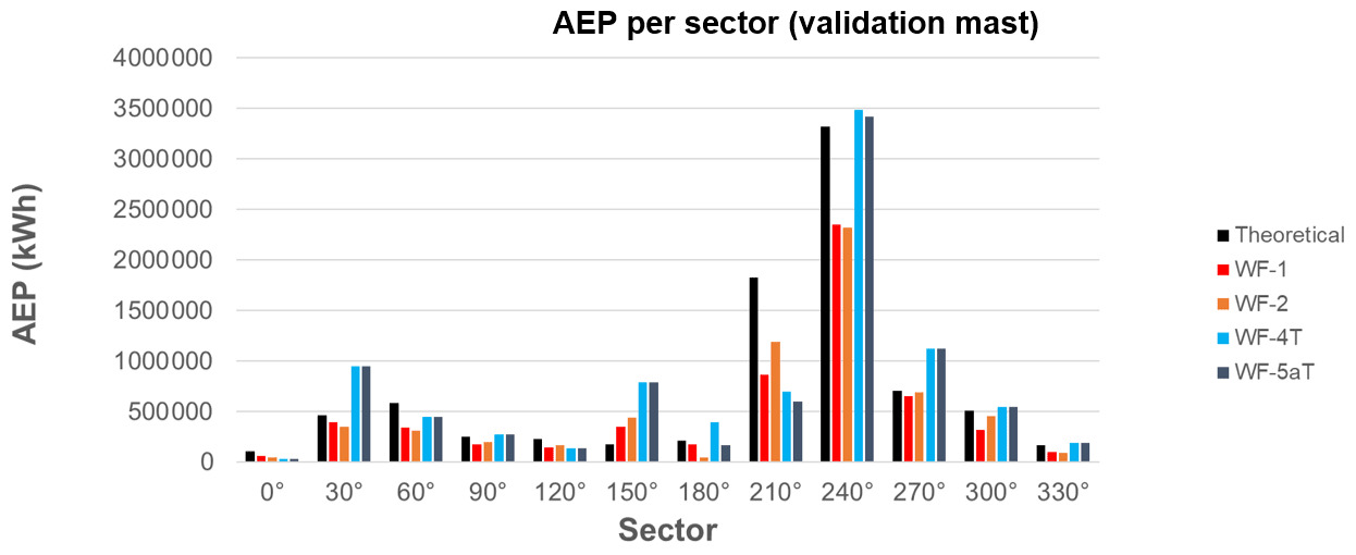
4.3 Site 3
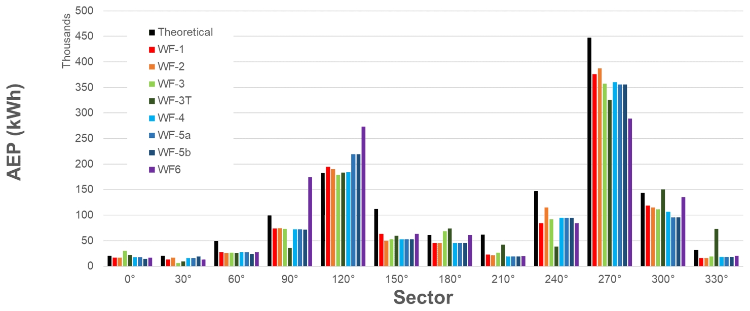
For this site, the AEP has been calculated at the validation location using the power curve of the Enercon E-40 wind turbine. This wind turbine has a rated power of 0.6 MW and a rated wind speed of 12 m s−1. A hub height of 50 m was assumed. The results in Fig. 13 show that the results are all underestimated, due to the underestimations of wind speeds in the most frequent sectors. The underestimation is quite consistent for all models (between 10 % and 15 %) except E-Wind, which underestimates the AEP by 24 %.
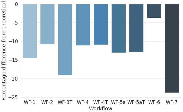
Figure 13Site 3 – percentage difference in gross AEP from the theoretical value for each workflow applied.
Details of the variations of the AEP for each wind direction sector can be found in the Appendix as well as in Barber et al. (2021). It was found that the AEP is significantly under-predicted in the most frequent sector (240∘), leading to an overall under-prediction of AEP. There is no particular pattern in the variation of AEP between each workflow. The very small effect of flow turning on the WF-4 and WF-5a (Fluent) results can be seen for some sectors.
4.4 Site 4
For this site, the AEP has been calculated at the validation location using the power curve of the Enercon E-82 wind turbine. This wind turbine has a rated power of 2 MW and a rated wind speed of 12.5 m s−1. The hub height is 78 m. The results in Fig. 14 show that, as opposed to the Site 3, the results for Site 4 are all overestimated, due to the overestimations of wind speeds in the most frequent sectors. The overestimation is largest for WF-4 (Fluent RANS), and the SBES simulation in WF-5a reduces this slightly. The effect of flow turning is minimal. The overestimation is small for WF-1 (WindPro) and WF-2 (WindSim).

Figure 14Site 4 – percentage difference in gross AEP from the theoretical value for each workflow applied.
Details of the variations of the AEP for each wind direction sector can be found in the Appendix as well as in Barber et al. (2021). It was found that the large over-prediction in AEP by the WF-3 and WF-4 workflows mainly occurs because of the over-prediction in the 240∘ sector, because this is the most frequently occurring sector. Additionally, it was found that an under-prediction of WF-1 (WindPro) and WF-2 (WindSim) in the 210∘ sector is probably compensated for by the over-prediction in 240∘, because both of these sectors occur for a similar proportion of time.
4.5 Site 5
For this site, the AEP has been calculated at the validation location using the power curve of the planned wind turbine type. The results shown in Fig. 15 match very well for WF-4T (Fluent RANS) and WF-5aT (Fluent SBES), with deviations less than 6 %. The WF-1 (WindPro) and WF-2 (WindSim) results are significantly lower, with deviations of 30 % and 26 %, respectively. These deviations may initially be surprising, considering that the wind profile RMSE values between simulations and measurements for the four workflows are similar. However, this has occurred because both under-predictions and over-predictions of the wind speed lead to a positive RMSE, whereas a combination of over-predicted and under-predicted wind speeds cancel each other out for the AEP calculation.
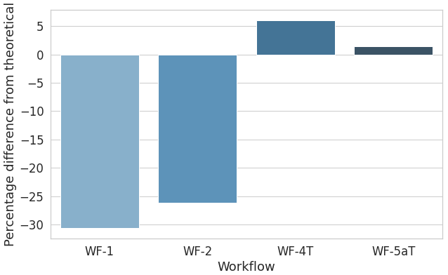
Figure 15Site 5 – percentage difference in gross AEP from the theoretical value for each workflow applied.
Details of the variations of the AEP for each wind direction sector can be found in the Appendix as well as in Barber et al. (2021). It was found that the AEP is particularly under-predicted in the 210∘ sector for all workflows, as well as in the 240∘ sector for WF-1 and WF-2, but not for WF-4T and WF-5aT.
Thus, the large difference in workflow results is attributed to the strongly under-predicted wind speed in the 240∘ sector of WindPro and WindSim. This has such a large influence on the AEP because of the very high average wind speeds in this sector combined with the high frequency of occurrence. It reveals an important point about this work – that the average absolute difference in wind speed over all sectors cannot be used as a reliable metric for the expected difference in AEP, even when it is weighted for the frequency of occurrence.
4.6 Comparison of wind speed and AEP results
In this section, the results of the simulated wind speeds and AEP calculations are compared by first plotting the error in simulated wind speeds against the error in expected AEP at the validation location for each site (Fig. 16). Each row corresponds to one site (from Site 1 to Site 5). The left-hand plots show the average error of all 12 wind speed direction sectors using a simple average, whereas the right-hand plots show the average error of all 12 wind speed direction sectors using an average weighted with wind speed frequency.
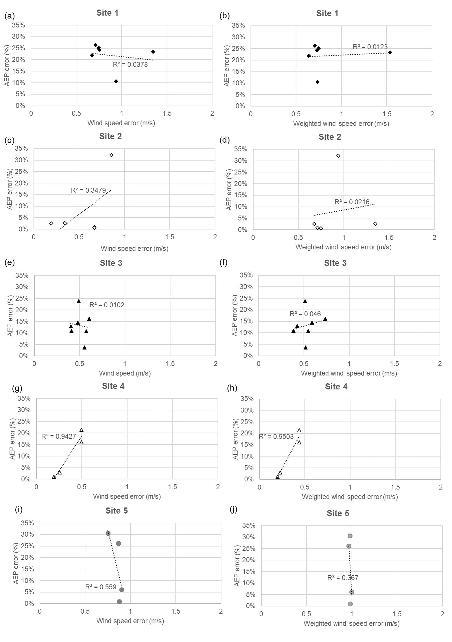
Figure 16Comparison of AEP errors to wind speed errors for all workflows and all sites for each site separately (a, c, e, g i: AEP compared to simple average wind speed; b, d, f, h, j: AEP compared to wind speed weighted for wind speed frequency.)
The correlation coefficients R2 are summarised in Table 10 for both a simple average of the wind speeds and for a weighted average. It should be noted that the low number of points in these correlations, especially for Site 4 with only four points, could lead to the low correlation coefficients. The results should therefore only be used indicatively rather the quantitatively. Generally, the correlation between wind speed error and AEP error is fairly low quality, with R2 ranging from 0.01 to 0.56 for Sites 1, 2, 3 and 5. The exception is Site 4, which has R2=0.94 for simple averaging and 0.95 for weighted averaging. The authors could find no particular reason why Site 4 should result in this significantly better correlation, except for the seemingly coincidental combination of a wide range of different effects that have come together to produce this result. The fact that Site 4 involved wind speed data directly from the wind turbine, rather than at a met mast, cannot explain this, unless the wind speeds were altered by the operator or manufacturer without the knowledge of the authors. The weighting does not have a large effect on the correlation coefficients and in some cases actually reduces the values. This indicates that the absolute value of the wind speed has a larger effect on the AEP accuracy than the actual accuracy in each sector and can be explained by the cubic relationship between wind speed and power. Figure 17 shows the results from all sites on a single plots – on the left for simple averaging and on the right for weighted averaging. This increases the overall correlation coefficient to 0.19 and 0.15 for simple averaging and weighted averaging, respectively.
Table 10Correlation coefficients and main set-up differences between wind speed and AEP errors for all sites.
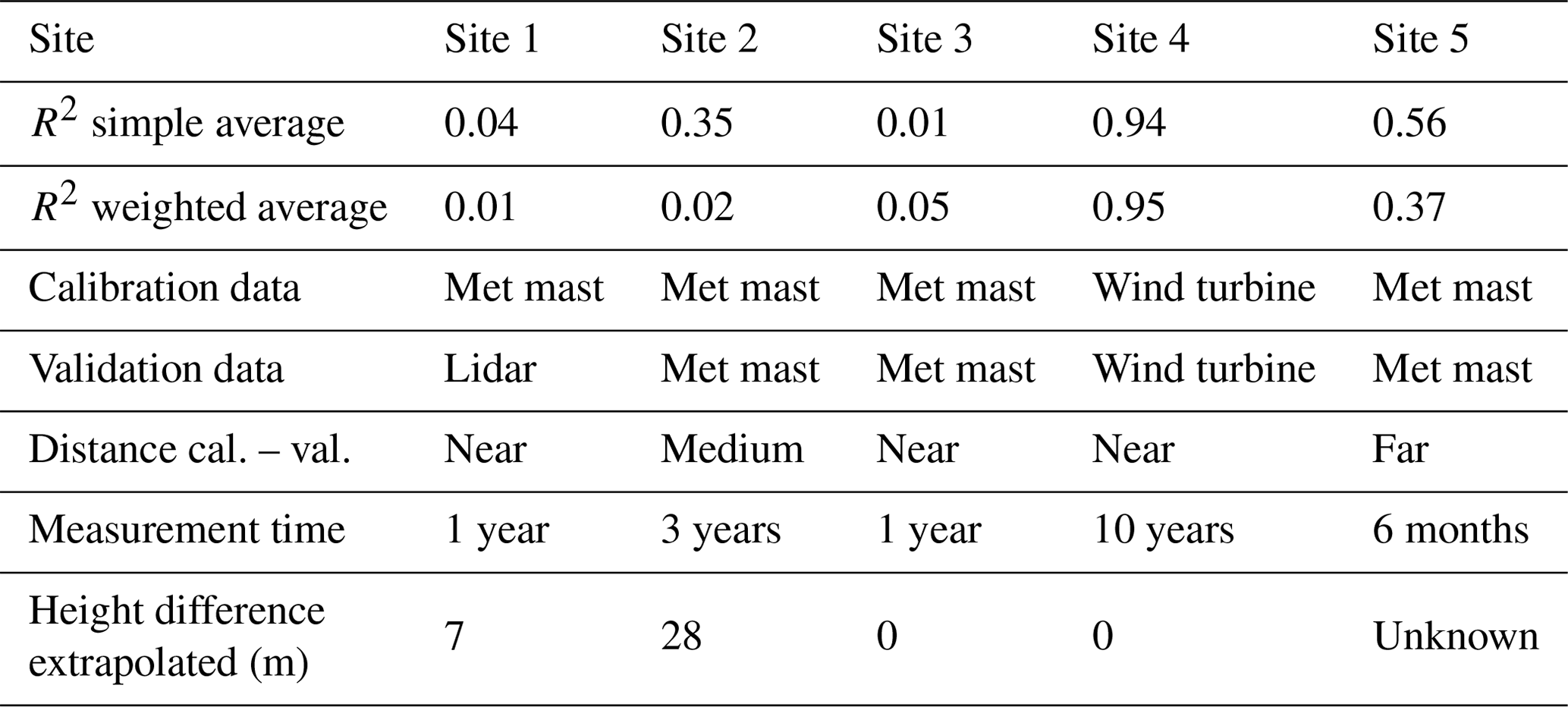
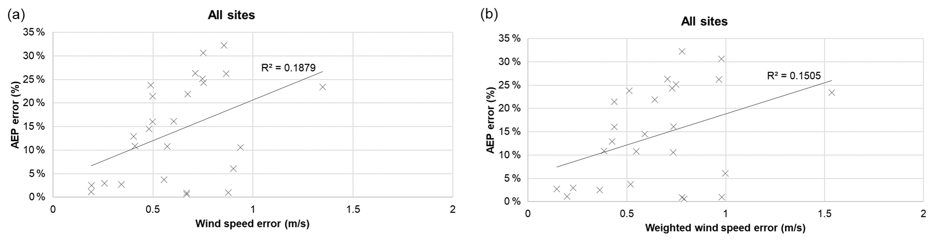
Figure 17Comparison of AEP errors to wind speed errors for all workflows and all sites: (a) AEP compared to simple average wind speed; (b) AEP compared to wind speed weighted for wind speed frequency.
For four out of five sites, there is no clear relationship between wind speed error and overall AEP error. Wind profile prediction accuracy does not translate directly or linearly to AEP accuracy. There could be several reasons for this. It could relate to the specific conditions at the site, to differences in workflow set-ups between the sites and to differences in workflow AEP calculation methods, as summarised below.
-
Specific site conditions:
-
The AEP depends strongly upon the relative strength and occurrence of the wind speed in the most commonly occurring wind direction sectors. The wind speed errors occurring in wind direction sectors that have high average wind speeds transfer to much higher errors in AEP due to the cubic dependency of power on wind speed. Furthermore, the wind speed errors occurring in wind direction sectors that have a higher frequency than other wind directions contribute more to the overall AEP errors. In some cases, these two situations compound, and wind speed errors occurring in wind direction sectors that have high average wind speeds and a high frequency of occurrence dominate the AEP errors. Conversely, high wind speed errors occurring in wind speed sectors that have low average wind speeds and/or low frequencies of occurrence become less important for the overall AEP error.
-
The site complexity is expected to affect the performance of the workflows in different ways for different wind direction sectors. For example, if a steep slope occurs between the calibration and validation locations in a particular wind direction, the accuracy will be reduced in this sector for flow models that cannot capture flow separation correctly. On the other hand, if a forest is located between the calibration and validation locations in a particular wind direction, the accuracy will be reduced in this sector for flow models that cannot correctly predict the canopy effect. This topic is discussed further in a separate paper by the same author (Barber et al., 2022), in which a new method for quantifying the complexity of a site is investigated.
-
-
Differences in workflow set-ups between the sites:
-
As mentioned in the introduction, this present study did not involve a systematic study of the effect of all calculation steps on the wind speed and AEP errors. This was due to the focus of the study on the relationship between cost and skill as can be seen in Barber et al. (2022). This means that it is not possible to quantify the effect of different set-ups on the correlation between wind speed and AEP errors. However, the main differences in workflow set-up between sites include type and accuracy of calibration and validation measurement, relative location of calibration and validation measurements, measurement time period, long-term extrapolation method, steepness of wind turbine power curve, vertical extrapolation method, and height difference between calibration and validation location. In further studies, these factors could be varied systematically for a range of sites. In Table 10, some of the main differences between the AEP calculation set-up between sites are summarised. However, no obvious relationship between the correlation quality and these factors can be seen.
-
-
Differences in workflow AEP calculation methods:
-
As shown in Table 2 in Sect. 2.1.5, differences in AEP calculation methods carried out by different organisations cannot be entirely ruled out and are expected to be larger between different workflows that have not been specifically compared and adjusted within a research project such as this one. A systematic study on this topic would be useful in order to quantify this effect.
-
As well as this, different AEP calculation methods exist and have been shown in Sect. 2.1.5 to have a significant effect on the AEP calculation. These differences can occur when different types and quality of data are available to different organisations. For example, the time series method can only be applied when time series data are actually available.
-
The combination of these different effects, and possibly others, leads to the results obtained in this work. Despite the fact that this work did not involve a systematic study of these effects, the importance of examining AEP errors as well as wind speed errors in any comparison study has been highlighted. As well as this, the complexity of the combined factors contributing to WRA errors has been demonstrated – even without including wake effects and other losses. The results show that the wind model that produces the most accurate wind predictions for a certain wind direction over a certain time period does not always result in the most suitable model for the AEP estimation of a given complex terrain site. In fact, the large number of steps within the WRA process often lead to the choice of wind model being less important for the overall WRA accuracy than would be suggested by only looking at wind speeds. Not only this, but additionally it is not immediately obvious which sites have a high correlation between wind speed and AEP errors and which ones do not. Future work will involve systematic studies of these effects.
It is therefore concluded that it is vitally important for researchers to consider overall AEP – and all the steps towards calculating it – when evaluating simulations of flow over complex terrain. This agrees with similar recent qualitative findings from the CREYAP2021 study (https://windeurope.org/tech2021/creyap-2021/, last access: 18 July 2022).
A range of simulations have been carried out with seven different wind modelling tools at five different complex terrain sites and the results compared to wind speed measurements at validation locations. The study was then extended to AEP estimations (without wake effects), and it was found that wind profile prediction accuracy does not translate directly or linearly to AEP accuracy. This could relate to the specific conditions at the site, to differences in workflow set-ups between the sites or to differences in workflow AEP calculation methods. Although a systematic study of the effect of all the possible varying factors was not done, the work highlighted the importance of examining AEP errors as well as wind speed errors in any comparison study. As well as this, the complexity of the combined factors contributing to WRA errors has been demonstrated – even without including wake effects and other losses. The results show that the wind model that produces the most accurate wind predictions for a certain wind direction over a certain time period does not always result in the most suitable model for the AEP estimation of a given complex terrain site. In fact, the large number of steps within the WRA process often lead to the choice of wind model being less important for the overall WRA accuracy than would be suggested by only looking at wind speeds. Not only this, but additionally it is not immediately obvious which sites have a high correlation and which ones do not. Future work will involve systematic studies of these effects. It is therefore vitally important for researchers to consider overall AEP – and all the steps towards calculating it – when evaluating simulations of flow over complex terrain.
The simulation tools used in this work are commercial tools. The AEP process tool used by OST is available on Zenodo at https://doi.org/10.5281/zenodo.6860048 (Schubiger et al., 2022).
The data sets used for this work are part of commercial projects and are not publicly available.
SB managed and coordinated the project and was responsible for writing the paper. AS carried out the Fluent simulations and developed the script for the AEP calculation process. SK and DE carried out the WindPro, WindSim and PALM simulations. ARa carried out the E-Wind simulations. ARu carried out the CFX simulations and developed the script for the AEP calculation process. HK supervised the work of ARu and provided valuable input for the paper.
The contact author has declared that none of the authors has any competing interests.
Publisher's note: Copernicus Publications remains neutral with regard to jurisdictional claims in published maps and institutional affiliations.
This work was carried out as part of the project “A new process for the pragmatic choice of wind models in complex terrain” funded by the Swiss Federal Office of Energy (SI/501807-01) and the German Federal Environmental Foundation (34933/01). We also thank the partner companies of this project for providing data and input about the simulated sites, including ewz, ADEV, and Enercon, as well as the Institut für Flugzeugbau at the Universität Stuttgart for providing us with the lidar data from the “Lidar complex” project.
This research has been supported by the Bundesamt für Energie (grant no. SI/501807-01) and the Deutsche Bundesstiftung Umwelt (grant no. 34933/01).
This paper was edited by Andrea Hahmann and reviewed by Andrea Vignaroli and one anonymous referee.
Alletto, M., Radi, A., Adib, J., Langner, J., Peralta, C., Altmikus, A., and Letzel, M.: E-Wind: Steady state CFD approach for stratified flows used for site assessment at Enercon, J. Phys.: Conf. Ser., 1037, 072020, https://doi.org/10.1088/1742-6596/1037/7/072020, 2018. a
Bao, J., Chow, F. K., and Lundquist, K. A.: Large-Eddy Simulation over Complex Terrain Using an Improved Immersed Boundary Method in the Weather Research and Forecasting Model, Mon. Weather Rev., 146, 2781–2797, https://doi.org/10.1175/MWR-D-18-0067.1, 2018. a
Barber, S., Buehler, M., and Nordborg, H.: IEA Wind Task 31: Design of a new comparison metrics simulation challenge for wind resource assessment in complex terrain Stage 1, J. Phys.: Conf. Ser., 1618, 062013, https://doi.org/10.1088/1742-6596/1618/6/062013, 2020a. a
Barber, S., Schubiger, A., Koller, S., Rumpf, A., Knaus, H., and Nordborg, H.: Actual Total Cost reduction of commercial CFD modelling tools for Wind Resource Assessment in complex terrain, J. Phys.: Conf. Ser., 1618, 062012, https://doi.org/10.1088/1742-6596/1618/6/062012, 2020b. a, b, c, d
Barber, S., Schubiger, A., Koller, S., Eggli, D., Rumpf, A., and Knaus, H.: A new process for the pragmatic choice of wind models in complex terrain, final report, Eastern Switzerland University of Applied Sciences, https://drive.switch.ch/index.php/s/DGxWeKQ35nnbPMW (last access: 18 July 2022), 2021. a, b, c, d, e, f, g, h, i
Barber, S., Schubiger, A., Koller, S., Eggli, D., Radi, A., Rumpf, A., and Knaus, H.: A New Decision Process for Choosing the Wind Resource Assessment Workflow with the Best Compromise between Accuracy and Costs for a Given Project in Complex Terrain, Energies, 15, 1110, https://doi.org/10.3390/en15031110, 2022. a, b, c, d
Bechmann, A., Sørensen, N. N., Berg, J., Mann, J., and Réthoré, P.-E.: The Bolund Experiment, Part II: Blind Comparison of Microscale Flow Models, Bound.-Lay. Meteorol., 141, 245–271, https://doi.org/10.1007/s10546-011-9637-x, 2011. a
Berg, J., Mann, J., Bechmann, A., Courtney, M. S., and Jørgensen, H. E.: The Bolund Experiment, Part I: Flow Over a Steep, Three-Dimensional Hill, Bound.-Lay. Meteorol., 141, 219–243, https://doi.org/10.1007/s10546-011-9636-y, 2011. a
Bowen, A. J. and Mortensen, N. G.: Exploring the limits of WAsP the wind atlas analysis and application program, in: European Union wind energy conference, edited by: Zervos, A., Ehmann, H., Helm, P., and Stephens, H. S., H. S. Stephens & Associates, Bedford, ISBN 0952145294, 1996. a, b
Jensen, N. O.: A note on wind generator interaction, Risø-M No. 2411, Risø National Laboratory, https://backend.orbit.dtu.dk/ws/portalfiles/portal/55857682/ris_m_2411.pdf (last access: 18 July 2022), 1983. a
Knaus, H., Rautenberg, A., and Bange, J.: Model comparison of two different non-hydrostatic formulations for the Navier-Stokes equations simulating wind flow in complex terrain, J. Wind Eng. Indust. Aerodynam., 169, 290–307, https://doi.org/10.1016/j.jweia.2017.07.017, 2017. a
Larsen, G. C.: A Simple Wake Calculation Procedure, Risø-M No. 2760, Risø National Laboratory. https://backend.orbit.dtu.dk/ws/portalfiles/portal/55567186/ris_m_2760.pdf (last access: 18 July 2022), 1988. a
Larsen, G. C., Madsen, H. A., Thomsen, K., and Larsen, T. J.: Wake meandering: a pragmatic approach, Wind Energy, 11, 377–395, https://doi.org/10.1002/we.267, 2008. a
Lee, J. C. Y. and Fields, M. J.: An overview of wind-energy-production prediction bias, losses, and uncertainties, Wind Energ. Sci., 6, 311–365, https://doi.org/10.5194/wes-6-311-2021, 2021. a, b
Liu, J., Chen, J. M., Black, T. A., and Novak, M. D.: E–ϵ modelling of turbulent air flow downwind of a model forest edge, Bound.-Lay. Meteorol., 77, 21–44, 1996. a
Menke, R., Vasiljević, N., Mann, J., and Lundquist, J. K.: Characterization of flow recirculation zones at the Perdigão site using multi-lidar measurements, Atmos. Chem. Phys., 19, 2713–2723, https://doi.org/10.5194/acp-19-2713-2019, 2019. a
Menter, F.: Zonal Two Equation k–w Turbulence Models For Aerodynamic Flows, https://doi.org/10.2514/6.1993-2906, 2012. a
Montavon, C.: Validation of a non-hydrostatic numerical model to simulate stratified wind fields over complex topography, J. Wind Eng. Indust. Aerodynam., 74–76, 273–282, https://doi.org/10.1016/S0167-6105(98)00024-5, 1998. a
Mortensen, N., Nielsen, M., and Ejsing Jørgensen, H.: Comparison of Resource and Energy Yield Assessment Procedures 2011–2015: What have we learned and what needs to be done?, in: Proceedings of the EWEA Annual Event and Exhibition 2015, European Wind Energy Association (EWEA), paper for poster presentation; EWEA Annual Conference and Exhibition 2015, 17–20 November 2015, Paris, France, https://backend.orbit.dtu.dk/ws/portalfiles/portal/118434032/Comparison_of_Resource_and_Energy_Yield_paper.pdf (last access: 18 July 2022), 2015. a, b
Mortensen, N. G., Landberg, L., Troen, I., and Lundtang Petersen, E.: Wind Atlas Analysis and Application program (WAsP): Vol. 1: Getting started, Risø-I No. 666(v.1)(ed.2)(EN), Risø National Laboratory, https://backend.orbit.dtu.dk/ws/portalfiles/portal/106061302/ris_i_666_EN_v.1_ed.2_.pdf (last access: 18 July 2022), 1998. a
Pozo, J. M., Geers, A. J., Villa-Uriol, M.-C., and Frangi, A. F.: Flow complexity in open systems: interlacing complexity index based on mutual information, J. Fluid Mech., 825, 704–742, https://doi.org/10.1017/jfm.2017.392, 2017. a
Richards, P. and Hoxey, R.: Appropriate boundary conditions for computational wind engineering models using the k–ϵ turbulence model, J. Wind Eng. Indust. Aerodynam., 46-47, 145–153, https://doi.org/10.1016/0167-6105(93)90124-7, 1993. a, b
Rodi, W. and Spalding, D.: PAPER 2 – A Two-Parameter Model of Turbulence, and its Application to Free Jets, in: Numerical Prediction of Flow, Heat Transfer, Turbulence and Combustion, edited by: Patankar, S. V., Pollard, A., Singhal, A. K., and Vanka, S. P., Pergamon, 22–32, https://doi.org/10.1016/B978-0-08-030937-8.50010-6, 1983. a, b
Sayre, R., Frye, C., Karagulle, D., Krauer, J., Breyer, S., Aniello, P., Wright, D. J., Payne, D., Adler, C., Warner, H., VanSistine, D. P., and Cress, J.: A New High-Resolution Map of World Mountains and an Online Tool for Visualizing and Comparing Characterizations of Global Mountain Distributions, Mount. Res. Dev., 38, 240–249, https://doi.org/10.1659/MRD-JOURNAL-D-17-00107.1, 2018. a
Schubiger, A., Hammer, F., and Barber, S.: WEST Wind Energy Simulation Toolbox, Zenodo [code], https://doi.org/10.5281/zenodo.6860048, 2022. a
Schulz, C., Klein, L., Weihing, P., Lutz, T., and Krämer, E.: CFD Studies on Wind Turbines in Complex Terrain under Atmospheric Inflow Conditions, J. Phys.: Conf. Ser., 524, 012134, https://doi.org/10.1088/1742-6596/524/1/012134, 2014. a
Wiernga, J.: Representative roughness parameters for homogeneous terrain, Bound.-Lay. Meteorol., 63, 323–363, 1993. a
Wood, N.: The onset of separation in neutral, turbulent flow over hills, Bound.-Lay. Meteorol., 76, 137–164, 1995. a
- Abstract
- Introduction
- Applied methods
- Simulation results – wind speeds
- Simulation results – annual energy production (AEP)
- Conclusions
- Appendix A: Appendix A1
- Code availability
- Data availability
- Author contributions
- Competing interests
- Disclaimer
- Acknowledgements
- Financial support
- Review statement
- References