the Creative Commons Attribution 4.0 License.
the Creative Commons Attribution 4.0 License.
 | 22 Jul 2022
Spatiotemporal observations of nocturnal low-level jets and impacts on wind power production
Stephanie Fiedler
A challenge of an energy system that nowadays more strongly depends on wind power generation is the spatial and temporal variability in winds. Nocturnal low-level jets (NLLJs) are typical wind phenomena defined as a maximum in the vertical profile of the horizontal wind speed. A NLLJ has typical core heights of 50–500 m a.g.l. (above ground level), which is in the height range of most modern wind turbines. This study presents NLLJ analyses based on new observations from Doppler wind lidars. The aim is to characterize the temporal and spatial variability in NLLJs on the mesoscale and to quantify their impacts on wind power generation. The data were collected during the Field Experiment on Submesoscale Spatio-Temporal Variability (FESSTVaL) campaign from June to August 2020 in Lindenberg and Falkenberg (Germany), located at about 6 km from each other. Both sites have seen NLLJs in about 70 % of the nights with half of them lasting for more than 3 h. Events longer than 6 h occurred more often simultaneously at both sites than shorter events, indicating the mesoscale character of very long NLLJs. Very short NLLJs of less than 1 h occurred more often in Lindenberg than Falkenberg, indicating more local influences on the wind profile. We discussed different meteorological mechanisms for NLLJ formation and linked NLLJ occurrences to synoptic weather patterns. There were positive and negative impacts of NLLJs on wind power that we quantified based on the observational data. NLLJs increased the mean power production by up to 80 % and were responsible for about 25 % of the power potential during the campaign. However, the stronger shear in the rotor layer during NLLJs can also have negative impacts. The impacts of NLLJs on wind power production depended on the relative height between the wind turbine and the core of the NLLJ. For instance, the mean increase in the estimated power production during NLLJ events was about 30 % higher for a turbine at 135 m a.g.l. compared to one at 94 m a.g.l. Our results imply that long NLLJs have an overall stronger impact on the total power production, while short events are primarily relevant as drivers for power ramps.
- Article
(8123 KB) - Full-text XML
- BibTeX
- EndNote


Renewable energy (RE) sources play an important role for meeting targets to mitigate climate change and to improve the access to electricity (Sadorsky, 2021). The RE sector is growing, and it is expected that its consumption will experience a 6.9 % compound annual growth rate in the new policies scenario between 2014 and 2040 (OECD/IEA, 2017). On a global scale, wind power has the potential to cover more than one third of the global energy demand until 2050 (IRENA, 2019). In the European Union, 80 % of the newly installed power capacities is RE technology, and wind power may become a main energy source after 2030 (OECD/IEA, 2017; Ziemann et al., 2020). In Germany, the share of RE to the overall installed power capacity is increasing continuously and largely stems from wind turbines already. A challenge for the success of the energy transition is the dependency of wind power production on meteorological conditions that vary in time and space (Frank et al., 2021; Druecke et al., 2021). This may cause power ramps associated with short-term increases or decreases in wind power production and variability on larger spatiotemporal scales associated with meso- to synoptic-scale weather phenomena.
This article focuses on nocturnal low-level jets (NLLJs) and their impacts on wind power. A NLLJ is a maximum in the vertical profile of the horizontal wind speed in the lower troposphere with a typical core between 50 and 500 m a.g.l. (above ground level) (Ziemann et al., 2020; Shapiro and Fedorovich, 2010). A past study of NLLJs in western Germany indicates that more than 16 % of NLLJs have a core below 200 m a.g.l., which is in the height range of most wind turbines (Marke et al., 2018). Typical hub heights of onshore wind turbines are 80 m to 140 m a.g.l. with rotor diameters of 80–118 m (Rohrig et al., 2019). A precise characterization, forecast and quantification of the uncertainty related to the wind speed at hub heights are crucial for wind power applications (Mirocha et al., 2016) and are needed for grid planning, financial calculations of operators (Rohrig et al., 2019) and site assessments for investors (Ziemann et al., 2020). In addition to the direct increase in the wind speed during NLLJ events, typically allowing increased power output (Abkar et al., 2016; Sharma et al., 2017), the NLLJ-related vertical wind shear (speed changes with height) and veer (directional shift with height) have also impacts on wind turbine power and reliability (Peña Diaz et al., 2012). The wind turbines may, for example, experience suboptimal or superoptimal power production, depending on shear and veer, getting to values of up to 5 % of the rated power for 1.5 MW utility-scale turbines (Wharton and Lundquist, 2012; Vanderwende and Lundquist, 2012; Murphy et al., 2020). Moreover, they impose additional static and mechanical loads on the rotor blades and shift wind turbine vibrations to higher amplitudes (Gutierrez et al., 2016), counteracting the wake effects (Ziemann et al., 2020; Doosttalab et al., 2020). Negative shear (decrease in the wind speed with height) produced by NLLJs at lower heights can also negatively affect wind turbines, which are usually designed assuming positive shear (Gutierrez et al., 2016). The partial presence of negative shear (and partially positive) in the rotor layer can slightly reduce the probability of damaging loads (Gutierrez et al., 2017), indicating that taller wind turbines, with rotors more often within the negative shear region of NLLJs, can be beneficial. The veer impacts are also directly related to the direction of the veer and the rotation of wind turbines (Englberger et al., 2020). Therefore, understanding positive and negative NLLJ impacts on wind turbines with different configurations plays an important role in the wind power industry.
NLLJs are a common phenomenon. Some NLLJ climatologies indicate a frequency of occurrence of about 10 % to 50 % of the nights, depending on the location and the identification criteria (Baas et al., 2009; Lampert et al., 2016). NLLJs were detected at one site in northern Germany, from May 2001 to April 2003, in 19 out of 29 different European synoptic weather patterns (Emeis, 2014), using the classification Großwetterlage (general weather situation) (James, 2007). Different meteorological conditions can generate NLLJs. The classically described development mechanism is associated with the decoupling of nocturnal winds from the surface friction by the formation of a near-surface temperature inversion (Blackadar, 1957). This condition typically happens at night, particularly on days with little cloud cover that allows strong radiative cooling of the surface. The classical theory describes the NLLJ formation using the concept of an inertial oscillation, a process tied to the decoupling of the air flow from surface friction. The associated weaker dynamical friction due to reduced eddy viscosity enables an acceleration of the air aloft (Ziemann et al., 2020; Fiedler et al., 2013), with the development of a pronounced super-geostrophic wind speed maximum in the course of the night (Shapiro and Fedorovich, 2010). Time and strength of the wind speed maximum depend of the geographical position and the time of decoupling. NLLJs also depend on horizontal pressure gradients in the mesoscale, commonly expressed as geostrophic wind (Beyrich et al., 1997; Salio et al., 2007). A near-surface temperature inversion paired with a sufficiently strong geostrophic wind can occur, for instance, at the edge of a mobile high-pressure system with an approaching extra-tropical cyclone. NLLJs typically start developing around sunset, coinciding with the development of a near-surface temperature inversion, and decaying with the onset of vertical mixing during the morning of the following day (Blackadar, 1957; Sisterson and Frenzen, 1978; Beyrich, 1994; Van de Wiel et al., 2010). Also, due to its lower intensity in the upper part of the daytime boundary layer and the largest ageostrophic wind component near ground, NLLJs occur first at higher heights, descending with time while increasing their strength (Beyrich et al., 1997).
Other NLLJ driving mechanisms than inertial oscillations are known. For instance, a NLLJ profile can be detected when an aged cold pool, e.g., generated by downdraft from deep moist convection, glides up over a radiatively formed stable boundary layer. The cold moist air settles then above the nighttime temperature inversion, where a NLLJ forms as the result of reduced frictional deceleration (Heinold et al., 2013). Another possibility is when a near-surface temperature inversion is formed by warm air advection over relatively cooler near-surface air. This happens when air from land is advected over a relatively cold sea during late spring or summer, which is important for offshore wind turbines (Kalverla et al., 2019; Svensson et al., 2019).
There is no past observational study that explores the driving mechanisms of NLLJs with detailed analyses of their duration, mesoscale extent and impacts on wind power. Past works on NLLJ characterization often had the limitation of rarely having measurements of vertical profiles for wind speed and direction on mesoscales, i.e., a few kilometers with a temporal resolution of minutes to hours. Wind properties are routinely measured at stations that are often located hundreds of kilometers apart such that mesoscale characteristics in space can not be analyzed. Such measurements are usually also limited to the height of meteorological masts, typically up to 100 m and sometimes up to 300 m, which are insufficient to fully characterize NLLJs. Another limitation is the representation of NLLJs in atmospheric models (Banta et al., 2002), e.g., those used for numerical weather predictions (NWPs) and reanalysis data. The models typically underestimate the strength and overestimate the height of NLLJs, while the wind veering between the surface and the top of the boundary layer is underestimated (Sandu et al., 2013; Svensson and Holtslag, 2009; Brown et al., 2005, 2008). Potential reasons are multiple and include the common artificial enhancement of the turbulent mixing during stable stratification to represent unresolved processes, e.g., vertical mixing associated with surface heterogeneity, gravity waves and sub-grid-scale variability (Sandu et al., 2013). Reanalysis data can share similar biases for the near-surface wind profile, and coarse vertical and spatial resolutions, including terrain discretization, are an additional contributing factor to those biases (Kalverla et al., 2019; Hallgren et al., 2020; Aird et al., 2021).
An opportunity to overcome these limitations is the deployment of Doppler wind lidars, which can continuously measure wind profiles with high vertical and temporal resolutions (Suomi et al., 2017). Doppler wind lidars emit laser beams in at least three different directions, which are scattered by aerosols. The measurements are used to determine the wind speed and direction based on the Doppler effect (Hallgren et al., 2020). Profiles of the mean wind speed are retrieved within the boundary layer and up to a few kilometers a.g.l., depending on the weather conditions. The quality of the wind retrieval depends on the amount of aerosols affecting the strength of the back-scattered signal (Pearson et al., 2009). In this work, we made use of new data from Doppler lidar instruments at two sites in eastern Germany. The two sites are about 6 km distant from each other, allowing the study of mesoscale spatiotemporal characteristics of NLLJs from June to August 2020. We detected NLLJs with an automated algorithm in this dataset and systematically assessed their mesoscale characteristics, driving mechanisms, including synoptic weather patterns, and impacts on wind power production.
2.1 FESST@home data
The Field Experiment on Submesoscale Spatio-Temporal Variability (FESSTVaL) (FESSTVal, 2020) is a joint field campaign organized by the Hans-Ertel-Centre for Weather Research and involving different partners. The primary goal of FESSTVaL is measuring sub-mesoscale to mesoscale variability by employing a measurement strategy to cover three main aspects: boundary layer patterns, cold pools and wind gusts. Measurements for FESSTVaL were carried out between January 2019 and December 2021. It included a test campaign in 2019, a remote campaign, FESST@home (due to the pandemic), at different locations in Germany during Summer 2020, and the main FESSTVaL campaign in spring and summer 2021. In the present study, we used the observational data from Doppler wind lidars deployed during FESST@home between June and August 2020. The lidars were installed and operated at the Lindenberg Meteorological Observatory – Richard Assmann Observatory (MOL-RAO) of the German Weather Service (DWD) located in Lindenberg (lat 52.21∘, long 14.13∘) and Falkenberg (lat 52.16∘, long 14.14∘), which are located 6 km apart from each other in a rural area in Brandenburg, east of Berlin. The terrain around the Falkenberg site is flat and surrounded by agricultural land. Lindenberg is located in a more complex area with some buildings and a small hill in the vicinity. For this work, data from three lidars were available: two (WL177 and WL78) located in Falkenberg and another (WL44) located in Lindenberg. All data have a temporal resolution of 10 min spanning partly different time periods (Table 1). The lidars operated in different measurement configurations. Lidar WL44 used the velocity azimuth display (VAD) method based on Päschke et al. (2015), WL177 operated in a gust mode with focus on temporally highly resolved wind measurements, inspired by Suomi et al. (2017) and documented in Steinheuer et al. (2022), and WL78 had a mode for measurements of turbulence parameters (Smalikho and Banakh, 2017). In addition to the lidars, Falkenberg also provides measurements from a meteorological mast up to 90 m a.g.l. for air temperature, wind speed and wind direction. The mast data were used for validating the lidar measurements and calculating the atmospheric stability.

Figure 1Data validation. (a) Comparison of the horizontal wind speed from the sonic anemometer against lidar WL177 at about 90 m a.g.l. The comparison in the azimuth range between 15 and 45∘ is shown in red to highlight the effects of the tower shadowing effect. (b) Pearson correlation coefficient (R) of the different lidars against the height a.g.l. WL177 and WL78 are located in Falkenberg, while WL44 is operated ∼6 km away in Lindenberg.
Table 1Location, operation mode, available number of days and periods with missing data of all instruments used to estimate the wind properties.

All lidar data were put through quality control. As the first step, wind profiles with less than 90 % of available data below 500 m were removed prior to the analysis. With this process, 3 %, 4 % and 6 % of the profiles from WL44, WL177 and WL78 were removed. In the second step, the lidar measurements were compared with the sonic anemometer data from 90 m a.g.l. in Falkenberg. Figure 1a shows the comparison for WL177. The other lidar in Falkenberg (WL78) had a similar behavior (not shown). We can see a dependence of the data agreement on the wind direction. The behavior is explained by the shadowing effect of the tower on the sonic anemometer for the 15 to 45∘ azimuth range (shown in red in Fig. 1a). We therefore removed the data in this azimuth range from the validation process. The resulting Pearson correlation coefficient R and the mean bias error (MBE) between the anemometer and the lidars are shown in Table 2. Both WL177 and WL78 obtained measurements closely correlated with the anemometer measurements with R=0.93. The correlation for WL44 is expected to be lower since the instrument is located at a distance of 6 km from the anemometer even though R=0.85 is relatively large. So, considering the anemometer measurements as the ground truth, the second step of the validation consisted in excluding lidar profiles with a wind speed difference larger than 20 % from the anemometer measurements (as in Hallgren et al., 2020). About 4 % of the remaining profiles from WL177 and WL78 were also excluded from this study. This step was not applied to WL44 in Lindenberg due to the large distance from the mast in Falkenberg.
Table 2Pearson correlation coefficient (R) and mean bias error (MBE) between the sonic anemometer and the different lidars at ∼90 m. On the left side, the measurements made in the azimuth range between 15 and 45∘ were excluded.
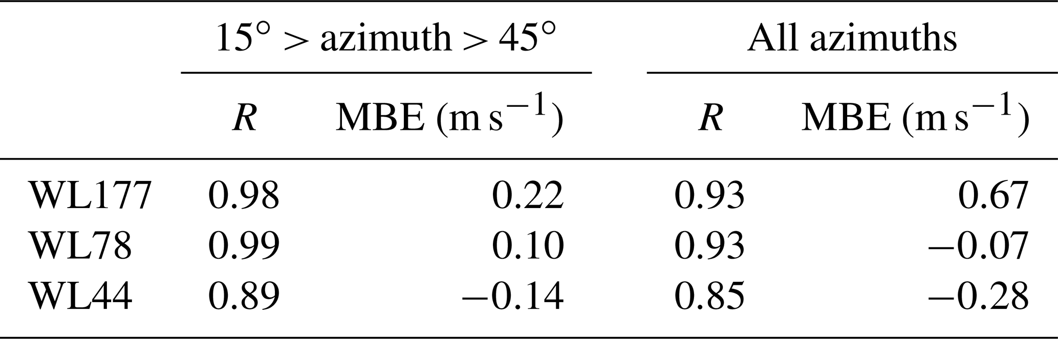
We further intercompared the entire wind profiles from the lidars by calculating the Pearson correlation R between the lidars at different heights (Fig. 1b). For this comparison, we interpolated all lidar data to the height levels of WL177, with a vertical resolution of 26.5 m. The exact procedure is explained in more detail in the next section. Both lidars in Falkenberg (WL177 and WL78) have R>0.98 between 53 m and 500 m a.g.l., while R for both WL177 and WL78 against WL44 is lower, with R around 0.94 between 100 and 1000 m a.g.l.. Note that R near the surface (here ∼26 m) is lower in all comparisons, consistent with the stronger influence from surface differences. Due to the similar results and the larger amount of data from WL177, in comparison to WL78, we used WL177 in most analyses. The lidar in Lindenberg (WL44) was used for assessing the spatial differences of NLLJs on the mesoscale. Hereafter, both WL177 and WL44 are called by the name of their location.
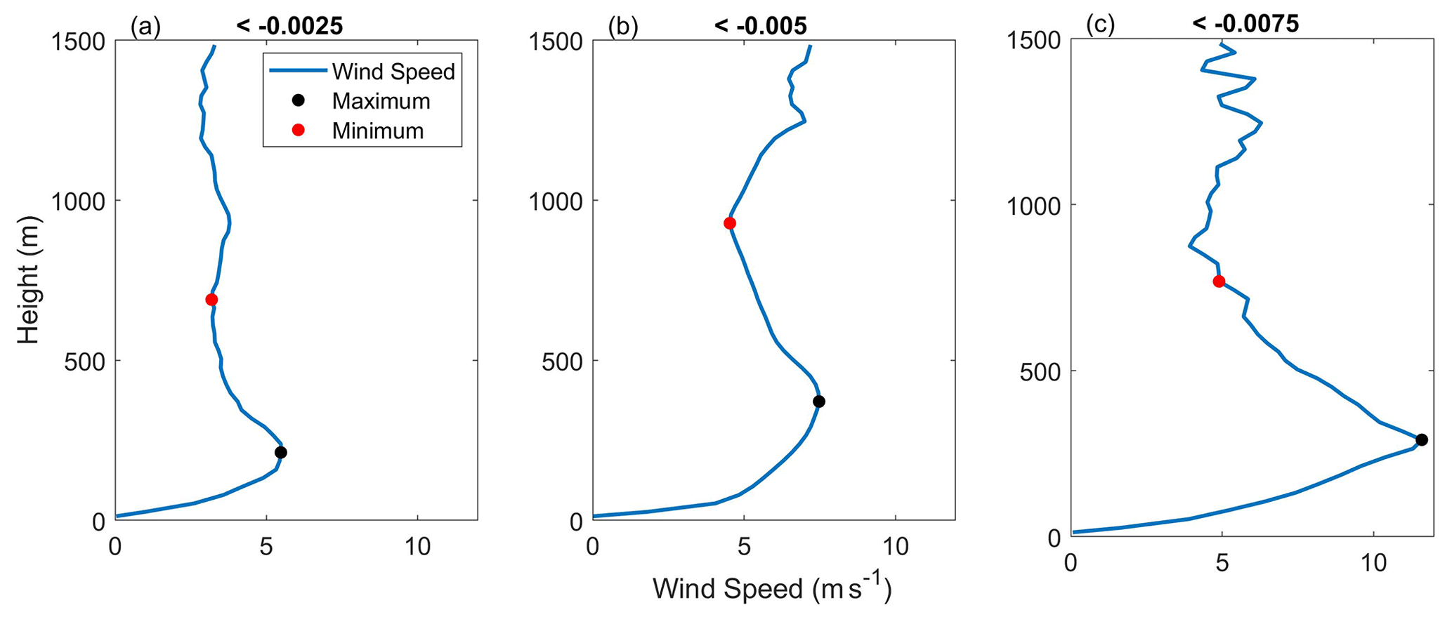
Figure 2Examples of NLLJ profiles identified with wind shear between the jet core and the minimum above it with the thresholds < −0.0025 s−1 (a), s−1 (b) and s−1 (c).
2.2 Automated NLLJ detection
We applied an automated detection algorithm for identifying NLLJs. Since there is no strict definition of a NLLJ, different methods for their identification have been proposed in the past. These include visual inspections of the profiles by eye (Emeis, 2014) and more objective methods using automated detection tools, e.g., a fall-off wind speed from the core of at least 2 m s−1 compared with the minimum value in the wind profile above (Hallgren et al., 2020) and additionally below (Andreas et al., 2000; Banta et al., 2002). Others use relative values, like a 25 % difference between the jet core and the minimum speed above (Baas et al., 2009; Wagner et al., 2019) or below (Tuononen et al., 2017). Some also include criteria for the maximum height and near-surface stratification (Fiedler et al., 2013), namely a jet core below 1500 m paired with a stably stratified surface layer of at least 100 m depth and a vertical wind shear stronger than −0.005 s−1 in the 500 m deep layer above the core. The first criterion was used to reflect the reduced frictional effects in the nocturnal boundary layer as pre-requisite for the formation of NLLJs. According to Aird et al. (2021), the use of a absolute criterion ensures that high-speed NLLJs are detected more reliably, and relative values can extract a higher number of NLLJs with lower wind speed maxima and higher duration.
Here, for the definition of the NLLJ automated detection criteria, only valid profiles with solar height lower than 0∘ from Falkenberg were analyzed. First, we smoothed the vertical profiles to avoid small and fast variability associated with turbulence in the measurements. To that end, we interpolated all lidar vertically onto a single coarse-grained height profile as the middle between every measurement height from WL177 in Falkenberg. This way we obtain the same vertical resolution of 26.5 m for all lidar data. Second, we calculated hourly moving averages for all wind profiles. Both these approaches successfully decreased the number of false detections of NLLJs, e.g., those that are extremely short or false alarms arising from turbulent motion causing maxima in the vertical wind profiles.
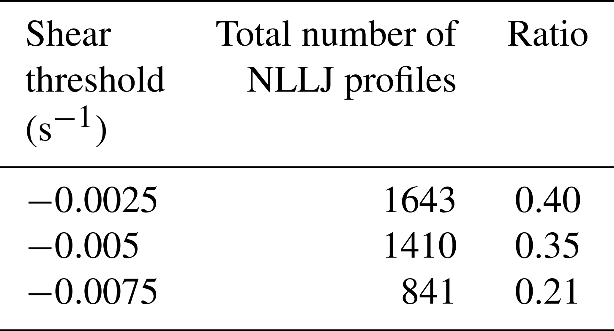
Our automatic identification of NLLJs was based then on detecting the NLLJ core as the wind speed maximum in the lowest 500 m deep layer and a critical mean vertical shear in the wind speed in a 500 m deep layer above the NLLJ core. Following past studies, we required a minimum wind speed difference of 2 m s−1 from the NLLJ core and the minimum above it and tested different mean threshold values for the vertical wind shear in the same layer. Figure 2 shows examples of NLLJ profiles identified with the tested shear criteria: , and s−1. The tests indicated a sensitivity of the number of detected NLLJs to the threshold for the shear criterion (Table 3), with the expected behavior that a weaker threshold resulted in more NLLJ identifications. Since the strongest threshold (−0.0075 s−1) might have missed relevant NLLJs for energy application, we chose the moderate setting of −0.005 s−1 for the shear threshold in the NLLJ detection.
Table 3Number of profiles flagged as NLLJ and the ratio of NLLJ profiles to all valid nocturnal profiles for different thresholds of the vertical shear in the horizontal wind speed.
For an easier characterization of the NLLJs, we filled 10 min gaps in between NLLJ detections; i.e., we flagged non-NLLJ profiles in between two NLLJ profiles also as a NLLJ. This approach allowed us a better estimation of the duration of NLLJ events excluding very short perturbations. We then removed all NLLJ events shorter than 30 min to exclude short-lived events.
Up to here, all NLLJs were detected at nighttime and thus for solar heights below 0∘. However, Fig. 3 shows a large presence of NLLJs also during daytime. To account for the full life cycle of NLLJs, we defined NLLJ nights as follows. Classical NLLJs can persist for up to a few hours after sunrise. We therefore calculated the ratio between early morning and late afternoon NLLJ detection for different solar heights, i.e., from 0∘ up to different positive solar heights. The chosen solar height for the definition of the NLLJ night was 20∘, with 92 % of the NLLJs occurring during early morning. The detection of a small number of NLLJs during late afternoon (8 %) might be associated with cold pools. During the campaign, the mean morning time for 0∘ (20∘) was 03:00 (05:00) UTC and for afternoon was 19:00 (17:00) UTC. All further analysis was made for solar heights smaller than 20∘, which was equivalent to an average period of about 12 h.
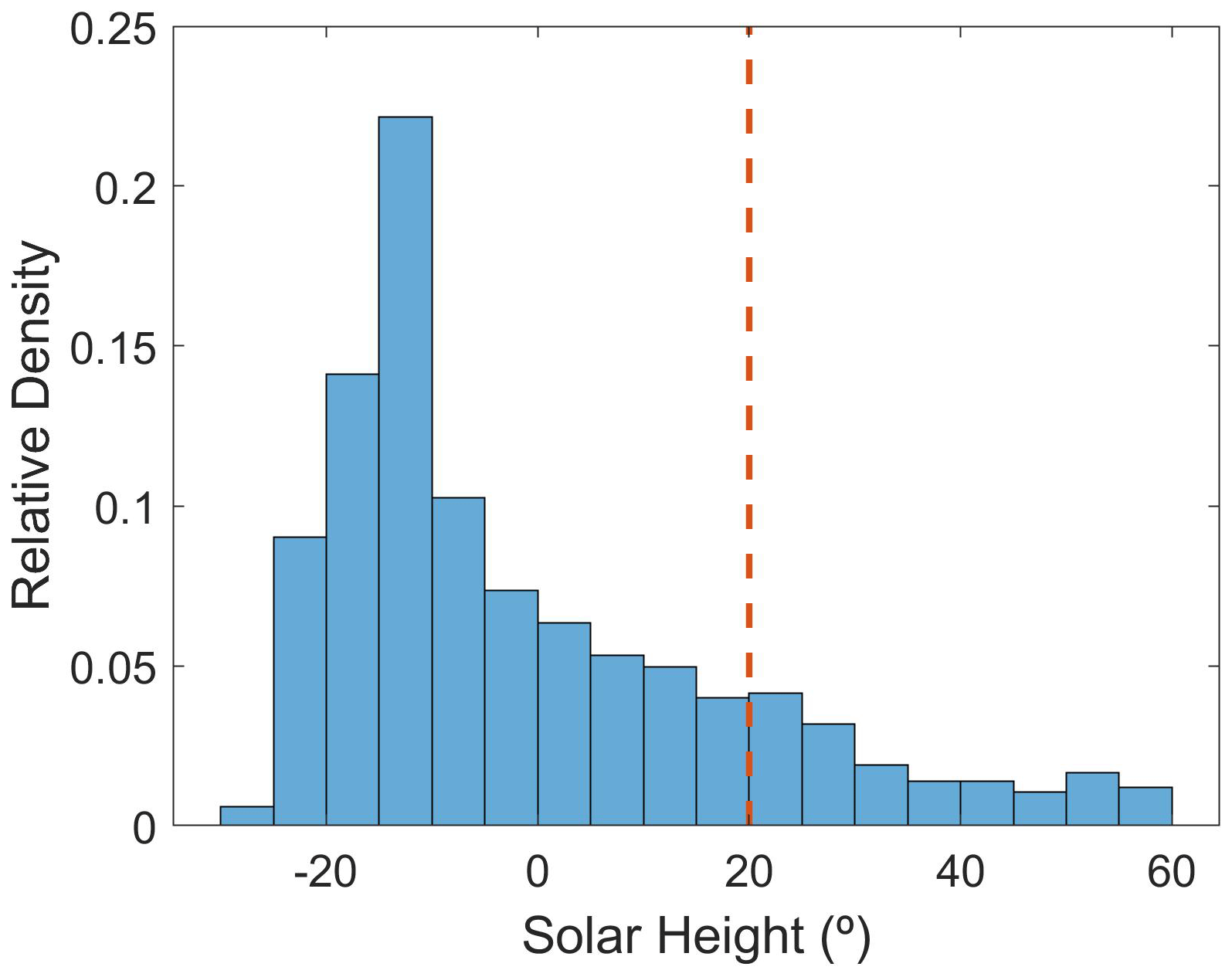
Figure 3Histogram of the relative density of NLLJs by solar height. The dashed red line represents the selected maximum solar height for the definition of a “NLLJ night”.
2.3 Atmospheric stability
For the atmospheric stability and the turbulent mixing of momentum, two different metrics were calculated using data from the mast between 1 and 10 m a.g.l. in Falkenberg. We calculated the temperature difference (dT) for the detection of near-surface temperature inversions as a measure of the static stability. Moreover, the Richardson number (Ri) was used to estimate the degree of turbulent mixing and the timing of downward mixing of momentum. Ri is calculated as the ratio of thermally induced turbulence and mechanically generated mixing by vertical wind shear:
where g=9.81 m s−1, θ is the potential temperature, V is the absolute horizontal wind speed, and h is the height a.g.l. In this work, we limited Ri values to ±3.5 since Ri can have very large or very small values, depending on the atmospheric conditions.
Large Ri values imply that the stratification is stronger than shear-driven mixing. Unstable conditions and turbulent mixing are associated with negative Ri values. The critical threshold for the transition between stable and unstable conditions is about 0.25 (Han et al., 2021); i.e., turbulence occurs when Ri is smaller than 0.25. These theoretical limits are fixed and do not depend on height. Ri can be small below the core of a strong NLLJ despite the stable thermal stratification, indicating mechanically driven turbulence by the strong vertical wind shear (Gutierrez et al., 2016).
2.4 Wind power production
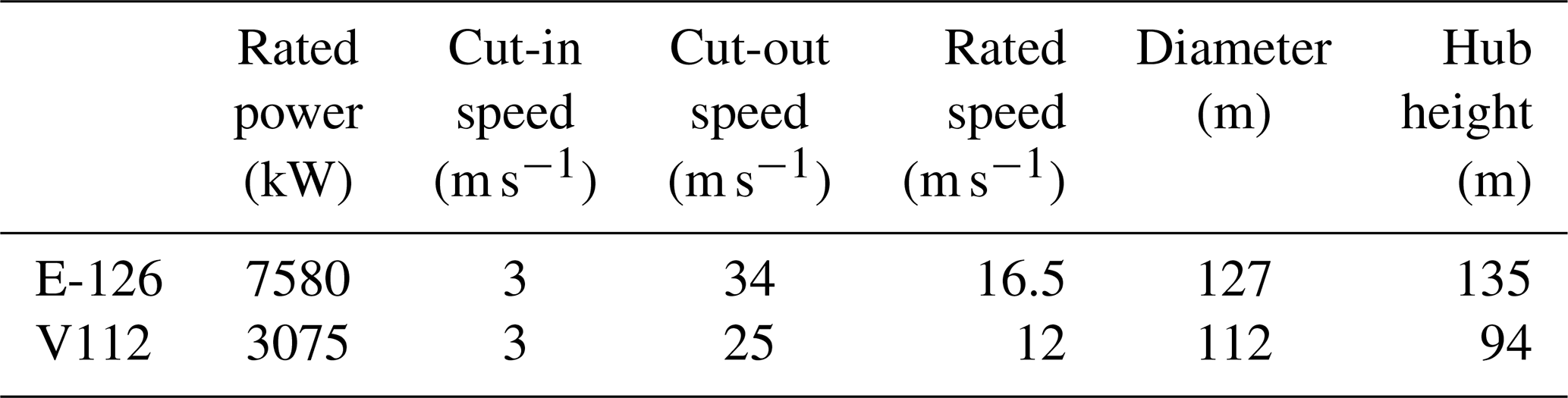
To quantify the impact of NLLJs on wind power production, we calculated the wind power production for two wind turbines: Enercon E-126 and Vestas V112 (Table 4). Their power curves (Figure 4) describe the wind power productions as a function of wind speed. The cut-in and cut-out wind speeds mark their different wind speed ranges for power production. For the power simulations, the wind speed from each lidar profile was interpolated to the hub heights of the wind turbines. It is known that factors other than the wind speed affect the power production. In this study, we estimated the stand-alone influence of wind speeds at hub height based on the power curves; everything else was kept constant. We further calculated the mean shear and veer in the mean rotor layer of ∼50–150 m, following Pichugina et al. (2017). The shear and veer were calculated as the mean wind difference per meter inside the rotor layer.
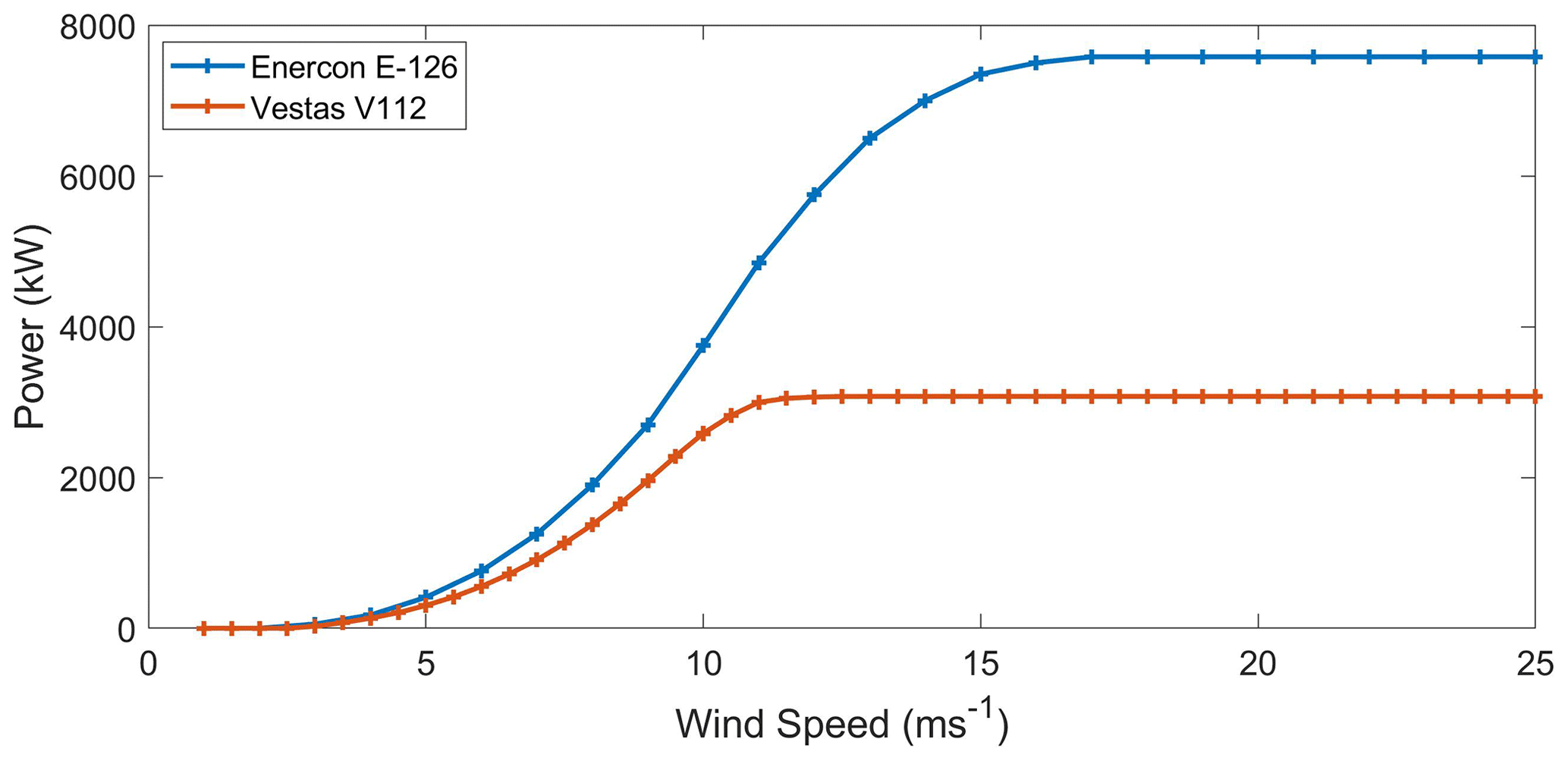
Figure 4Power curves of the Enercon E-126 and Vestas V112 Onshore turbines. The E-126 turbine still produces energy until its cut-out wind speed of 34 m s−1.
Table 4Characteristics of the Enercon E-126 and Vestas V112 Onshore wind turbines.
3.1 Statistics of NLLJs
The mean occurrence frequency of NLLJs was similar at both measurement sites, indicating NLLJs are a typical mesoscale event – here at least in the sub-class meso-gamma (2–20 km). The frequency of occurrence of NLLJ profiles in Falkenberg was 29 %, calculated by dividing all identified NLLJ profiles (1839) by the total of valid observed nocturnal wind profiles (solar height < 20∘). The frequency of occurrence in Lindenberg was 23 %, slightly lower, with a total of 1607 profiles classified as NLLJs.
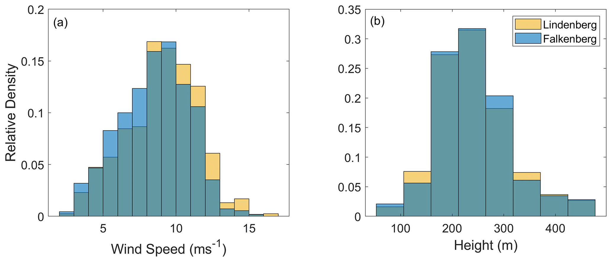
Figure 5NLLJ core wind speed (a) and height (b) in Falkenberg (blue) and Lindenberg (yellow).
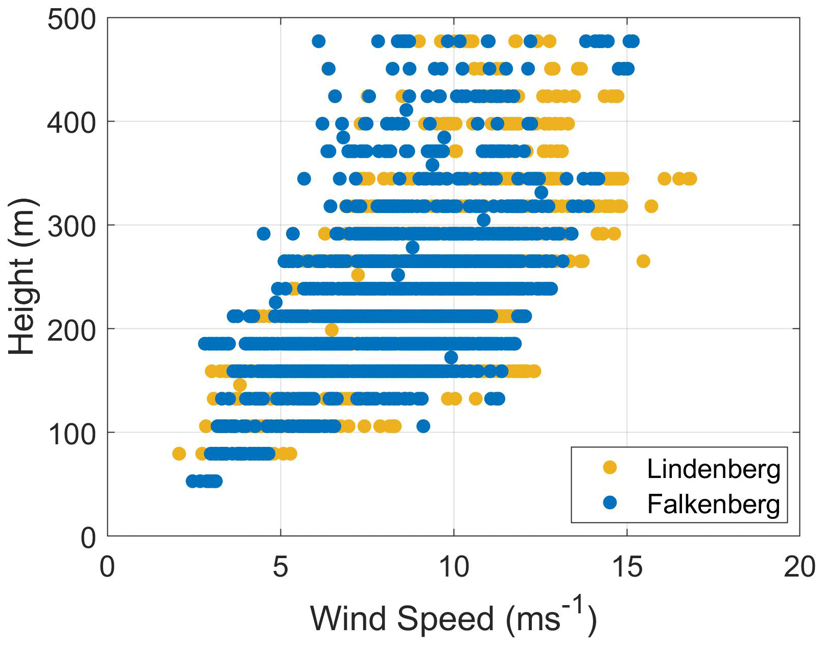
Slightly stronger NLLJs occurred in Lindenberg than Falkenberg, but the NLLJ core heights were very similar at both places (Fig. 5) and indicated a clear increase in the wind speed with height (Fig. 6). The mean wind speed at the jet core was of 8.5 (9.0) m s−1, with a minimum of 2.5 (2.1) m s−1 and a maximum of 15.2 (16.8) m s−1 in Falkenberg (Lindenberg). The mean jet core height was 229.9 (224.1) m, with a minimum of 53 (79.5) m and a maximum of 477 (477) m. In most cases, the height of the NLLJ cores was below 300 m. Interestingly, the horizontal wind speed and height distributions of the NLLJs shown here were similar to statistics from Braunschweig (about 250 km to the west) during the summer months in 2013 (Ziemann et al., 2020). Even Pichugina et al. (2017) identified NLLJs with a mean wind speed of 9.4 m s−1 and mean height of 149.3 m a.g.l. on the east coast of the USA.
Looking at the duration of NLLJ events revealed more apparent differences across the two sites. Figure 7 shows a histogram with the length of the NLLJ events at both places. The minimum NLLJ duration was 30 min due to the applied data filtering, and the maximum duration was about 11 h, limited by the duration of the surface inversion. The time span with the largest number of NLLJ profiles was 0.5 to 3 h. Lindenberg was affected by a larger number of NLLJ events shorter than 1 h.
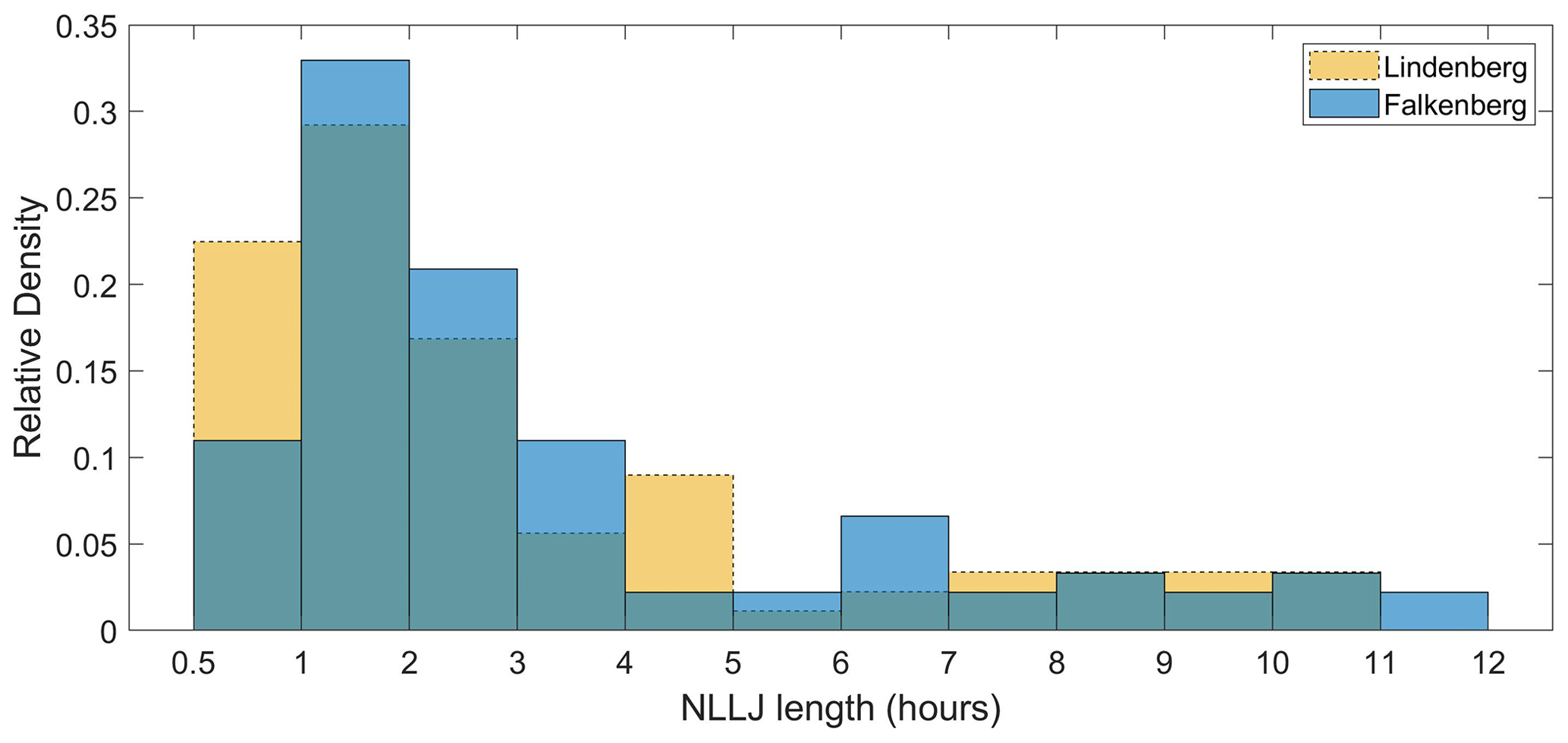
Figure 7Lengths of NLLJs color-coded for the two sites. The data filtering implies that events shorter than 30 min are removed prior to the data analysis.
3.1.1 Short vs. long events
Comparing the NLLJ wind speeds and heights for long events (>3 h) and short events (≤3 h) at both sites highlighted different behaviors. The mean jet core wind speed of long events was stronger, 7.8 (8.4) m s−1 against 6.1 (7.0) m s−1 in Falkenberg (Lindenberg), but the extremes were more frequent for short events (Fig. 8). The highest NLLJs were also the ones that were typically short. Also, the mean core height at 222.9 (218.8) m for long NLLJs was a bit lower than for short events at 244.3 (236.0) m in Falkenberg (Lindenberg). From Fig. 8 we can also see that the longer events had narrower distributions.
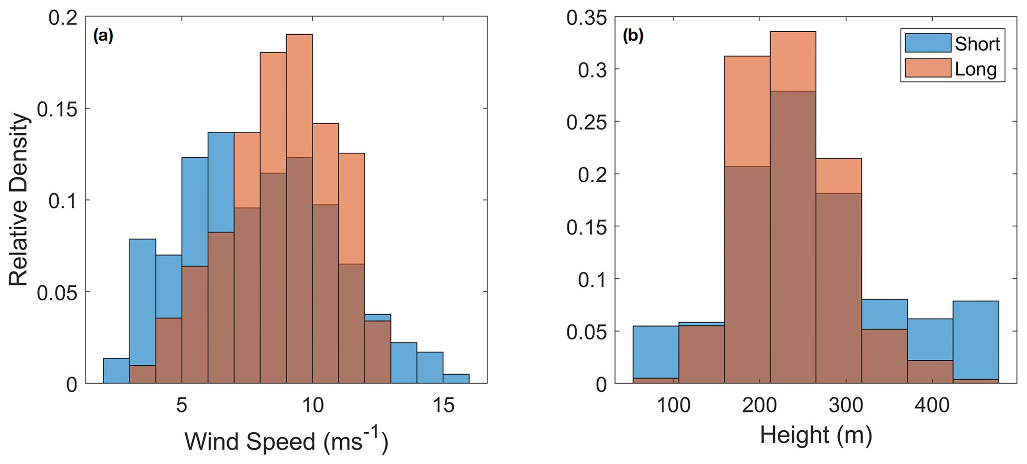
Figure 8Frequency of NLLJ core wind speeds (a) and heights (b) in Falkenberg during short (≤3 h) and long events (>3 h).
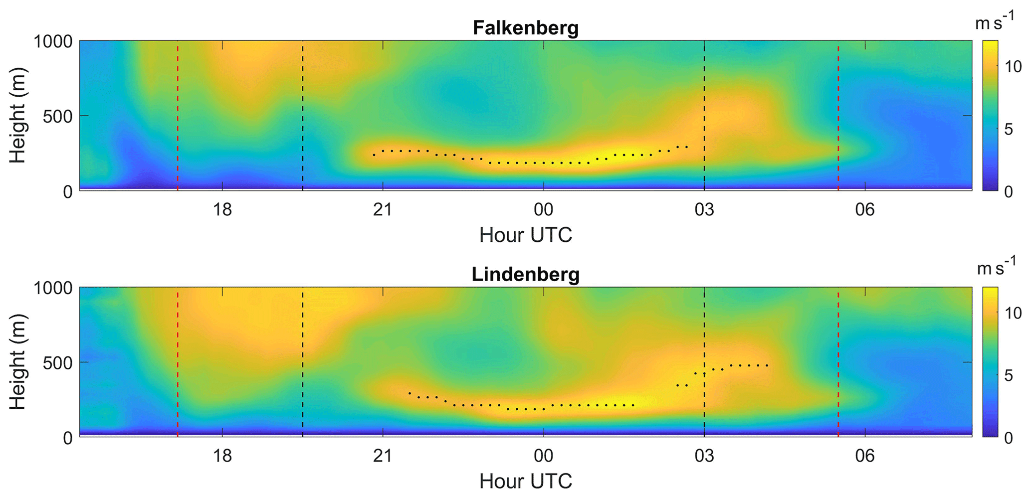
Figure 9Absolute wind speed (m s−1) during the night between 27 and 28 June 2020 in Falkenberg and Lindenberg as a function of time and height a.g.l. The black dots mark the NLLJ core and dashed black (red) lines the time of 0∘ (20∘) solar elevation.
Table 5Total number and percentage of nights with at least one NLLJ event and the number of nights with NLLJs classified by their duration. The percentage for the four latter columns are calculated from the number of all NLLJ nights.
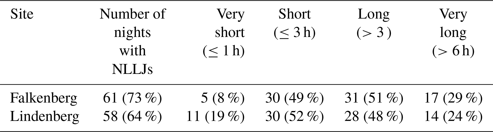
Table 5 shows the number of nights with at least one NLLJ event, as well as the number of nights with NLLJs classified by their duration. The percentage in brackets is the frequency of occurrence of NLLJs relative to the total number of nights (first column) and relative to the total number of NLLJ nights (latter four columns). We can see that 73 % (64 %) of the nights presented at least one NLLJ event in Falkenberg (Lindenberg) with a clear division of about half of those nights having events longer than 3 h. The presence of very long events (>6 h) was similar at both locations at 24 % and 29 % of the NLLJ nights, but the number of nights with only very short events (≤1 h) was more than doubled in Lindenberg (11) compared to Falkenberg (5).
3.1.2 Co-occurring events
Furthermore, we compared co-occurring NLLJs from both lidars. This assessment was inspired by the example of a long NLLJ that occurred during the night of 27–28 June 2020 at both locations but developed differently over time (Fig. 9). While the nocturnal development was very similar between 22:00 and 02:00 UTC, there were differences during the early morning. Falkenberg saw a single long NLLJ that persisted until around 02:00 UTC when the NLLJ detection in Lindenberg was interrupted. In Lindenberg, the NLLJ was detected again around 03:00 UTC but not in Falkenberg. Such differences are associated with intermittent mixing and reflect the local differences in meteorological conditions and possibly the terrain. To better understand such effects, we assessed the spatial differences of co-occurring NLLJ profiles at both sites next.
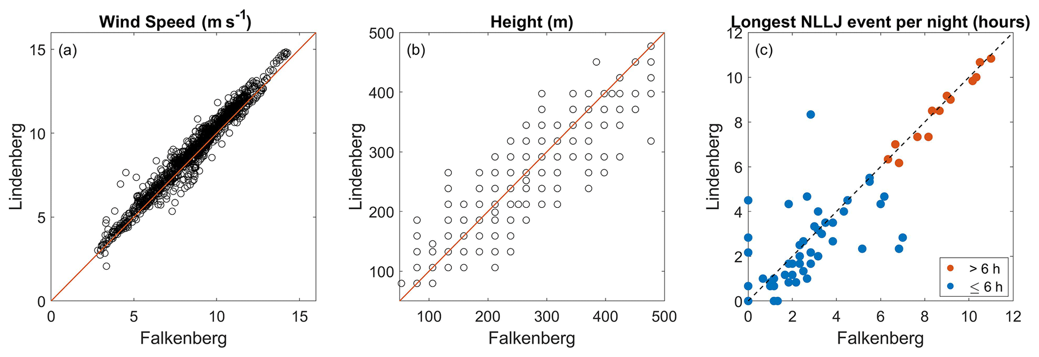
Figure 10Characteristics of co-occurring NLLJs at the two sites. Shown are (a) core wind speed, (b) core height and (c) lifetime of the longest NLLJs per night. In (c), events longer than 6 h at both sites are shown in red.
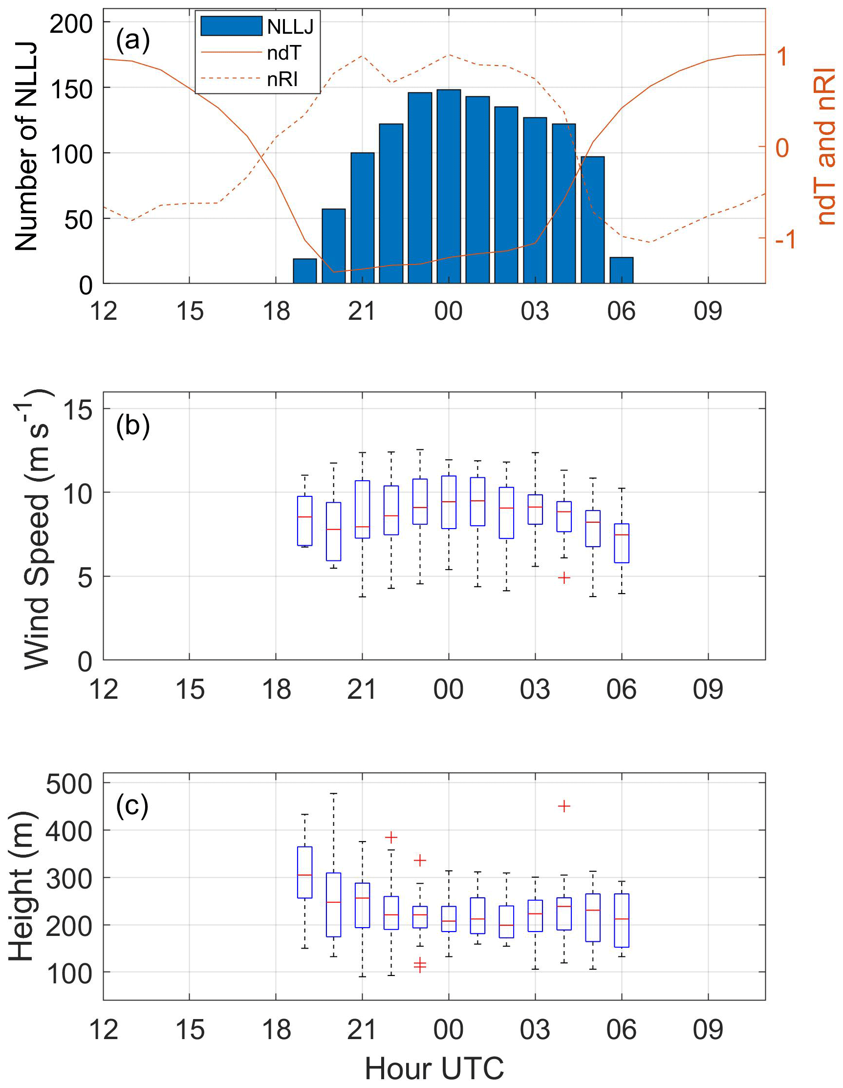
Figure 11Daily cycle of NLLJs in Falkenberg. Shown are (a) the number of long NLLJs per hour, (b) their core wind speed and (c) their core height. Lines in (a) show the hourly averaged and normalized Ri (nRi) and dT (ndT).
We performed a statistical comparison of the core wind speed and height for co-occurring NLLJ profiles at the two sites (Fig. 10a and b). While the wind speeds were often similar at both places, the heights had larger differences between the two places. From the NLLJ profiles identified in Falkenberg, 75 % were also identified in Lindenberg, while for the opposite it was 87 %, underlining the frequent co-occurrence of NLLJs on the mesoscale. Restricting the analysis to short NLLJ events, the percentages were smaller, with values of 48 % and 53 %. This is to be expected since short NLLJ events can be associated with intermittent developments of long NLLJs (as in Fig. 9), driven by density currents from convective cold pools that may not affect both sites simultaneously or even driven by local conditions like terrain differences. This behavior was also reflected in the lifetime of co-occurring NLLJs at the two sites (Fig. 10c). Co-occurring NLLJs lasting for more than 6 h had typically similar lifetimes at both places. This is consistent with the mesoscale spatial extent of NLLJs being driven by reduced frictional coupling of the wind field with surface friction in an inertial oscillation.
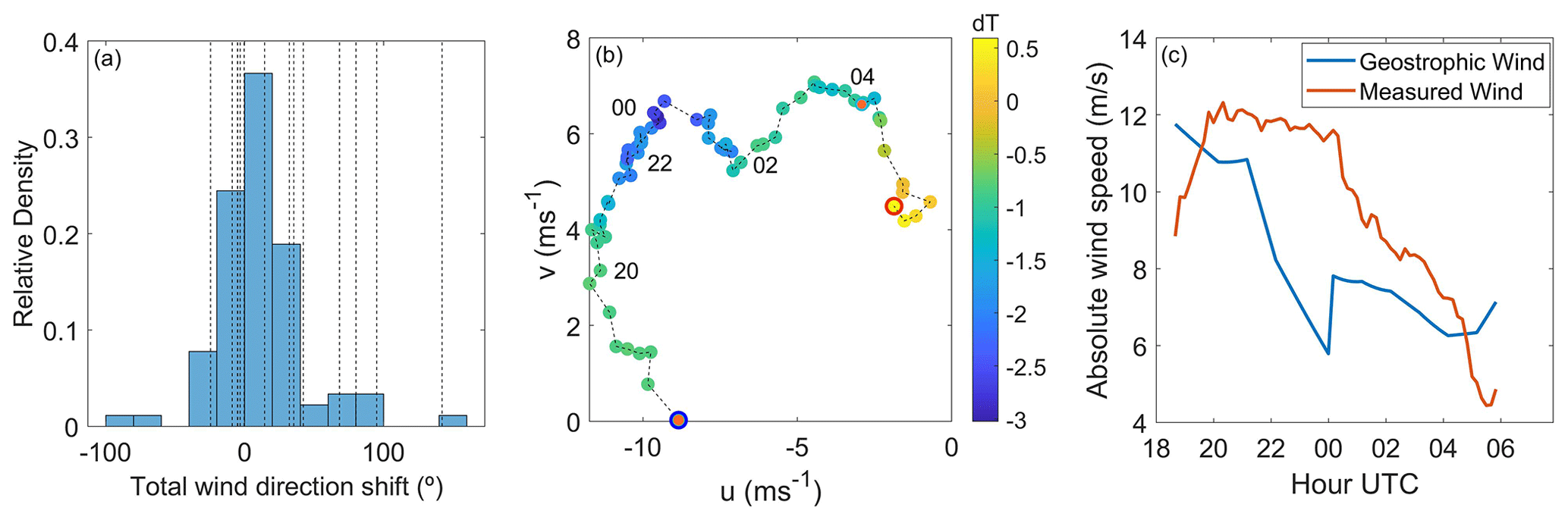
Figure 12Directional shifts during NLLJ development. Shown are (a) frequency of the total wind direction shift in the NLLJ cores for Lindenberg, (b) the zonal (u) and meridional (v) wind components during the NLLJ in the night of 12–13 August 2020 in Falkenberg, and (c) the actual and geostrophic wind speed. In (a) positive values mean a clockwise shift, and dashed lines mark the total directional shift during the very long NLLJs. In (b) the color illustrates the vertical temperature change (dT) in the first 10 m a.g.l., and the blue (red) circle marks the start (end) of the NLLJ. The additional orange circles mark the sunset and sunrise, and the numbers are the UTC times. The geostrophic wind in (c) was calculated from ERA5 data (Hersbach et al., 2020) and interpolated to the measurement times.
3.1.3 Temporal development
Looking at long NLLJ events in more detail revealed a nocturnal development similar to what one expects from inertial oscillations. Figure 11 shows the daily cycles of long NLLJs, including distributions of the jet core speed and height, as well as the normalized mean Ri (nRi) and dT (ndT) between 1 and 10 m a.g.l. The normalization was made by dividing the mean hourly values by their maximum positive values in order to better illustrate the daily cycle. The development of long NLLJs depended on the presence of the near-surface temperature inversion. Take for instance the temperature gradient ndT in Fig. 11a. After sunset, ndT increased, indicating the development of a surface inversion and leading to a reduction in frictional effects on the air flow at some distance from the surface. Stable stratification prevailed until the early morning hours when NLLJs also frequently occurred. It is important to mention that the average nRi and ndT had similar behavior when we included nights without NLLJs. This is a reflex of the higher stability of the atmosphere during night time. We also saw an increase in the mean core wind speed over time up to about 01:00 UTC when it started to decrease until the early morning. Up to 23:00 UTC, the mean jet height decreased and remained about constant thereafter. This behavior is broadly consistent with the process expected for an inertial oscillation, but there are also differences as would expected from the idealized assumption of stationarity in the theory. For example, longer periods of increasing wind speed are predicted from the theory, coinciding with half a period of the oscillation in mid-latitudes (approx. 8 h; Van de Wiel et al., 2010). This difference from the theoretical duration was apparent, especially for the short events. In addition to non-stationarity, reasons for differences between the measurements and the theory are the neglection or simplification of the smaller, yet still present, frictional effects (Blackadar, 1957; Van de Wiel et al., 2010). In reality, NLLJs are affected by intermittent mixing events, i.e., temporally variable frictional coupling of the jet with the surface layer and changes in the geostrophic wind along with the synoptic-scale weather conditions.
The wind directions changed in the course of the development of NLLJs but not as systematic as one would expect for a classical inertial oscillation. We selected the data from Lindenberg for quantifying the changes in wind direction in the core of the NLLJs. Most NLLJ events did not show large changes in wind direction in the course of their lifetime, falling between −40 and 40∘ total directional changes calculated as the total wind direction shift in the NLLJ core. NLLJs more frequently had a clockwise change (positive values in Fig. 12a) than counterclockwise. An inertial oscillation causes the wind field to veer in the course of the night. One therefore expects a larger directional shift in the NLLJ wind the longer the events are. We identified a total shift in the direction of the mean absolute values of 34∘ for short events, 107∘ for long events and 132∘ for very long events, consistent with veering in an inertial oscillation. Indeed, some of the longest events (marked by dashed lines in Fig. 12a) had large wind directional shifts, consistent with the theory of an undisturbed inertial oscillation.
The turning of the wind is very clear for the longest NLLJ event in Lindenberg during the night of 12–13 August 2020 (Fig. 12b). The NLLJ development began around sunset shortly after 18:00 UTC and ended due to turbulent mixing in the early morning hours (04:00–06:00 UTC), indicated by the morning time increase in dT. The perturbations in the turning of the wind are clearly related to fast changes in the geostrophic wind at about 00:00 UTC. This relationship between wind-turning perturbations and fast geostrophic wind changes also happens to other events from the campaign (not shown). This NLLJ event also led to supergeostrophic wind speeds consistent with the theory (Fig. 12c). The supergeostrophy, although already expected from theory, might at least in parts be explained by the slackening geostrophic winds in this example. Thus, changes in the synoptic-scale conditions affected the NLLJ development, although this event is close to characteristics expected from the theory. Other NLLJ events showed larger deviations from the theory (not shown), indicative of intermittent turbulence perturbing the nocturnal acceleration and turning of the wind field paired with temporal changes in the horizontal pressure gradients due to the evolving weather. The NLLJ of 12–13 August 2020 was associated with an anticyclonic southeasterly wind over the measurement sites due to a high-pressure system to the northeast.
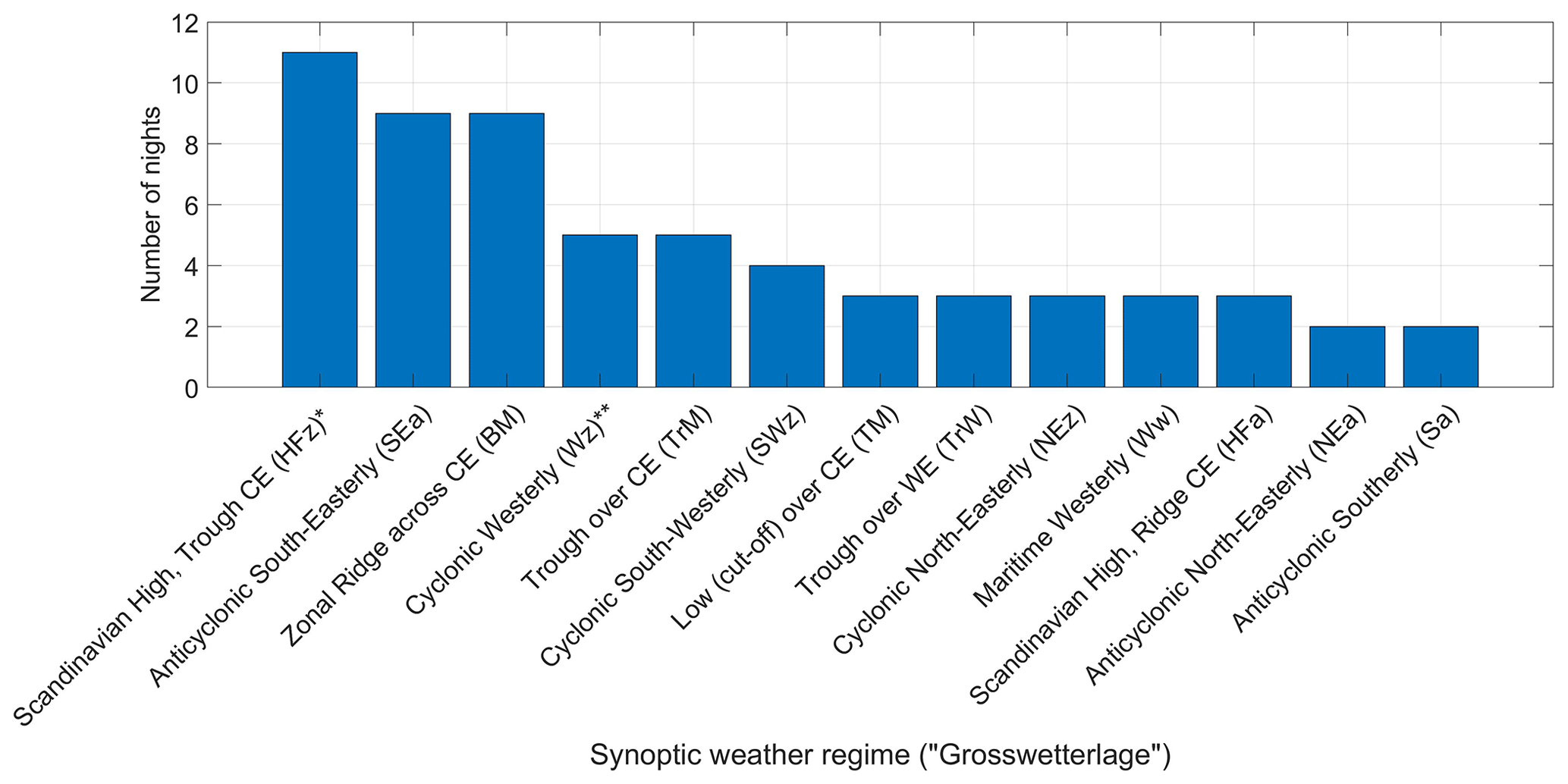
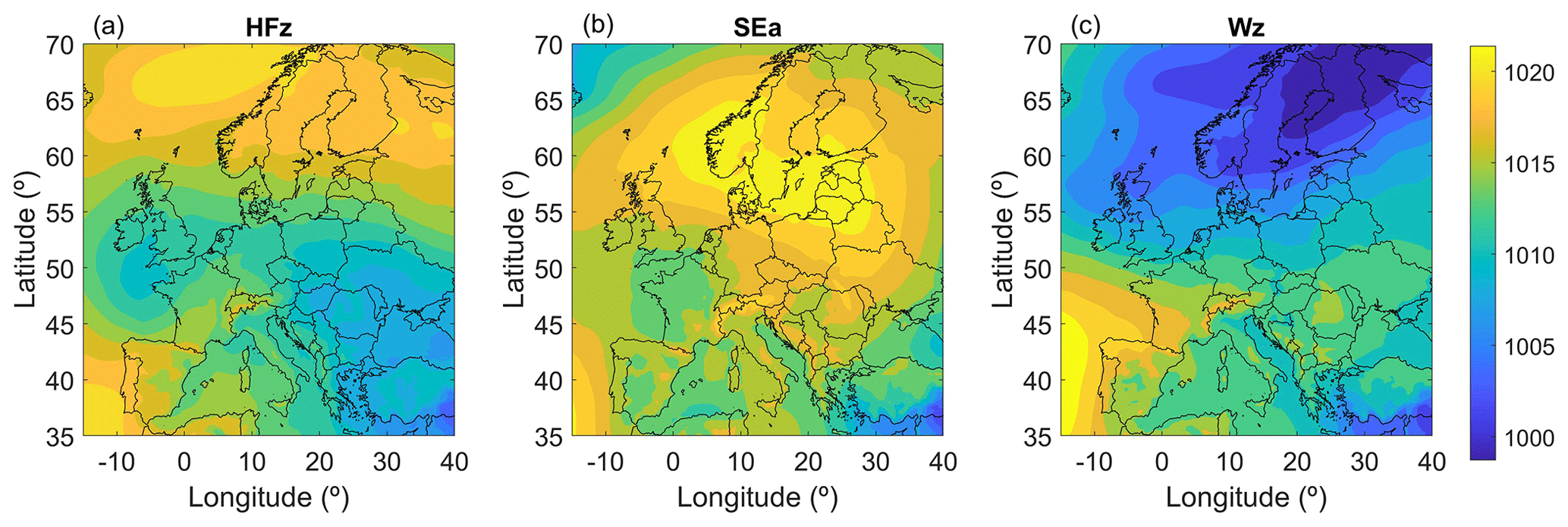
Figure 14Weather patterns favorable for NLLJ development. Shown are composites of the 00:00 UTC mean sea level pressure patterns during FESST@home for the weather patterns: (a) Scandinavian high, trough central Europe (HFz), (b) anticyclonic south-easterly (SEa) and (c) cyclonic westerly (Wz). The mean sea level pressure data were obtained from ERA5 reanalysis (Hersbach et al., 2020).
3.1.4 Weather patterns
We systematically investigated the occurrence of NLLJs under different synoptic weather patterns. Using the Großwetterlagen of the German Weather Service (James, 2007), we detected NLLJs in 13 out of 16 different weather pattern occurrences (Figure 13). Three weather patterns had particularly favorable conditions for NLLJ development. The pattern with the largest amount of NLLJ events was the Scandinavian high, trough central Europe (HFz) pattern (Fig. 14a). The most efficient pattern was the anticyclonic south-easterly (SEa, Fig. 14b), with the highest overall probability, since all nine cases were associated with a NLLJ. Both weather patterns point to inertial oscillations being driven by the sufficiently large geostrophic wind at the margin of a high-pressure system paired with relatively dry conditions allowing stronger nocturnal radiative cooling of the surface. The two synoptic weather patterns are shown as composites in Fig. 14a and b, indicating high-pressure systems in northern Europe and lower pressure towards the south resulting in a large horizontal pressure gradient over the measurement site. The pattern with the largest number of short NLLJ events was the cyclonic westerly (Wz) (Fig. 14c), pointing to NLLJs associated with the passage of low-pressure systems. Northeast Germany was also found in a zone with a strong pressure gradient during this weather pattern.
These results are broadly consistent with findings by Emeis (2014), based on data from May 2001 to April 2003 in Hanover (about 300 km to the west from our sites). They indicate that a short period can be sufficient to assess NLLJs associated with different weather patterns, although longer datasets would be needed for a full climatological assessment. It is interesting that we detected NLLJs during two patterns that were not detected in the previous study, namely cyclonic north-easterly (NEz) and anticyclonic north-easterly (NEa). These differences may be related to the different NLLJ identification methods, different locations or different time periods. In Emeis (2014), SEa also had a very high efficiency; however, the high Scandinavia-Iceland, ridge central. Europe (HFNa), with the highest efficiency in his work, did not occur during our campaign.
3.2 Effects of NLLJ on wind power generation
3.2.1 Power generation
NLLJs have a strong effect on wind power generation since they increase the wind speed at rotor heights. We quantified these effects using wind data at 100 m a.g.l. from lidar WL177 in Falkenberg, representative of typical rotor hub heights (Fig. 15a). The frequency distribution of these hub wind speeds during NLLJ events is clearly shifted to higher values compared to all data. For instance, the mean hub wind speed of 4.8 m s−1 from all data is smaller than the mean of 6.0 m s−1 during NLLJ events.
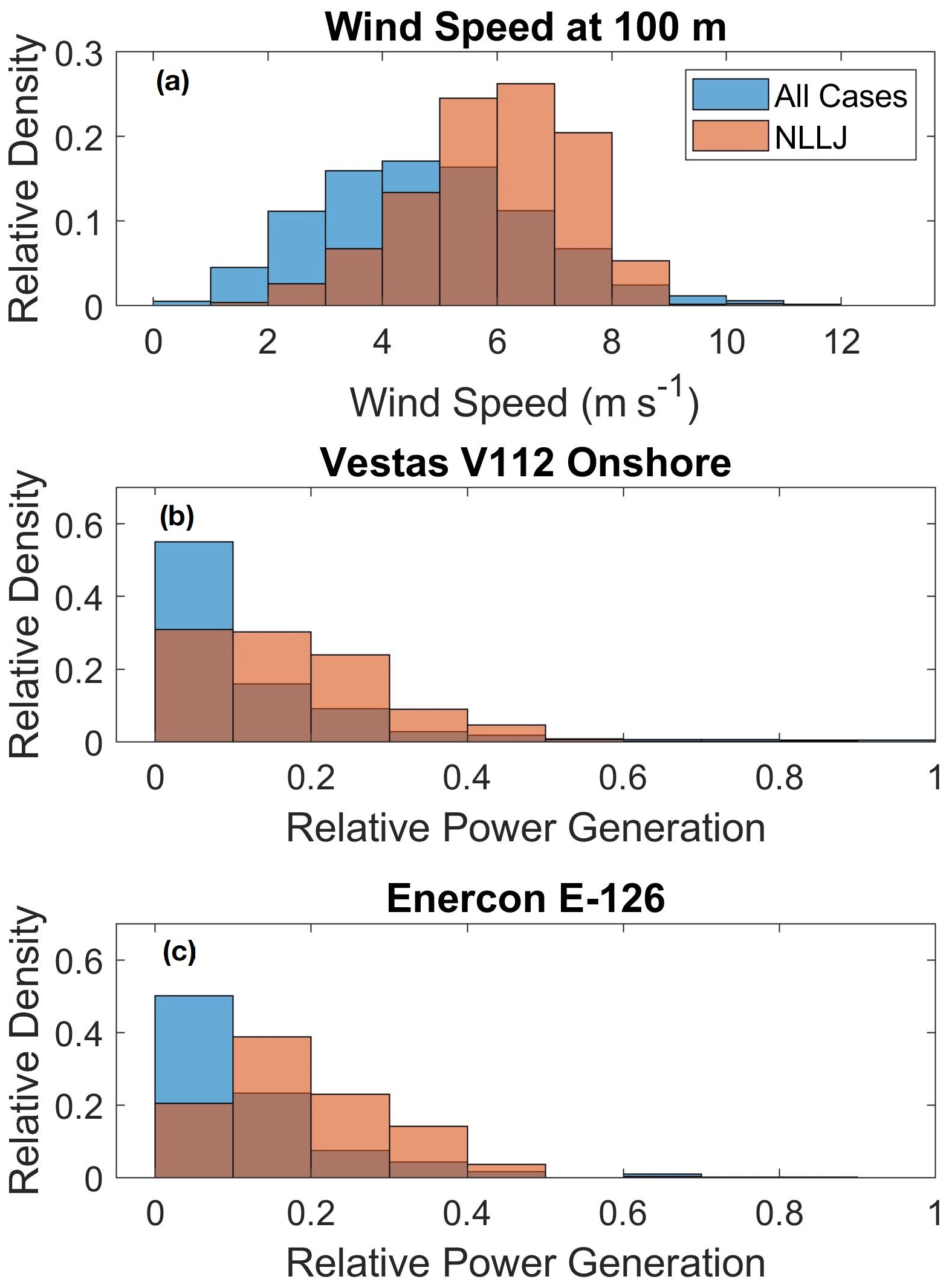
Figure 15Wind power production associated with NLLJs. Shown are the frequency of (a) the wind speed at 100 m a.g.l. and the relative power production from (b) E-126 and (c) V112 for all cases (blue) and NLLJ conditions (red). The relative power generation was calculated relative to the rated power of the turbine types.
We calculated the wind power generation from two wind turbine models: Enercon E-126 and Vestas V112. The former has a much larger rated power and steeper increase in power generation with wind speed. We therefore normalized the wind power estimates by the respective rated power of the turbine for a better comparability of the results (Fig. 15b and c). The results highlighted the shift in the frequency distribution of wind power generation to higher values during NLLJ events. The distributions reflect the production in the lower half of the power curve since the wind speed rarely reached values needed for yielding the rated power.
The additional power generation during NLLJs nonlinearly depends on the turbine type. From the estimated total wind power potential during the campaign, 24 % (28 %) was generated during NLLJ conditions for the V112 (E-126). NLLJs increased the mean power generation of the same turbines by 53 % (80 %) compared to all conditions. This implies mean power values of 382.2 (583.3) kW for V112 and 785.2 (1412.2) kW for E-126 during all conditions (NLLJs). In comparison, the changes in wind speed at rotor heights were not as strong: 23 % for V112 and 32 % for E-126. This behavior reflects nonlinear dependencies of the power generation on NLLJ occurrence and characteristics, depending on the turbine type and hub height. Power production from the higher wind turbines with larger rated power therefore benefits more strongly from the occurrence of NLLJs.
Weak NLLJs (e.g., Fig. 16d) were rare such that most NLLJs were strong enough to reach the cut-in wind speed of both wind turbines and allowed power generation. We observed NLLJ profiles with wind speeds below the cut-in threshold at the rotor heights of the E-126 (135 m) in 12 individual profiles, translating to 0.2 % of all valid NLLJ profiles. For the V112 (94 m) this happened for 45 profiles or 0.7 %. These differences between the two turbine types are primarily explained by the different rotor heights since the cut-in wind speeds are identical.
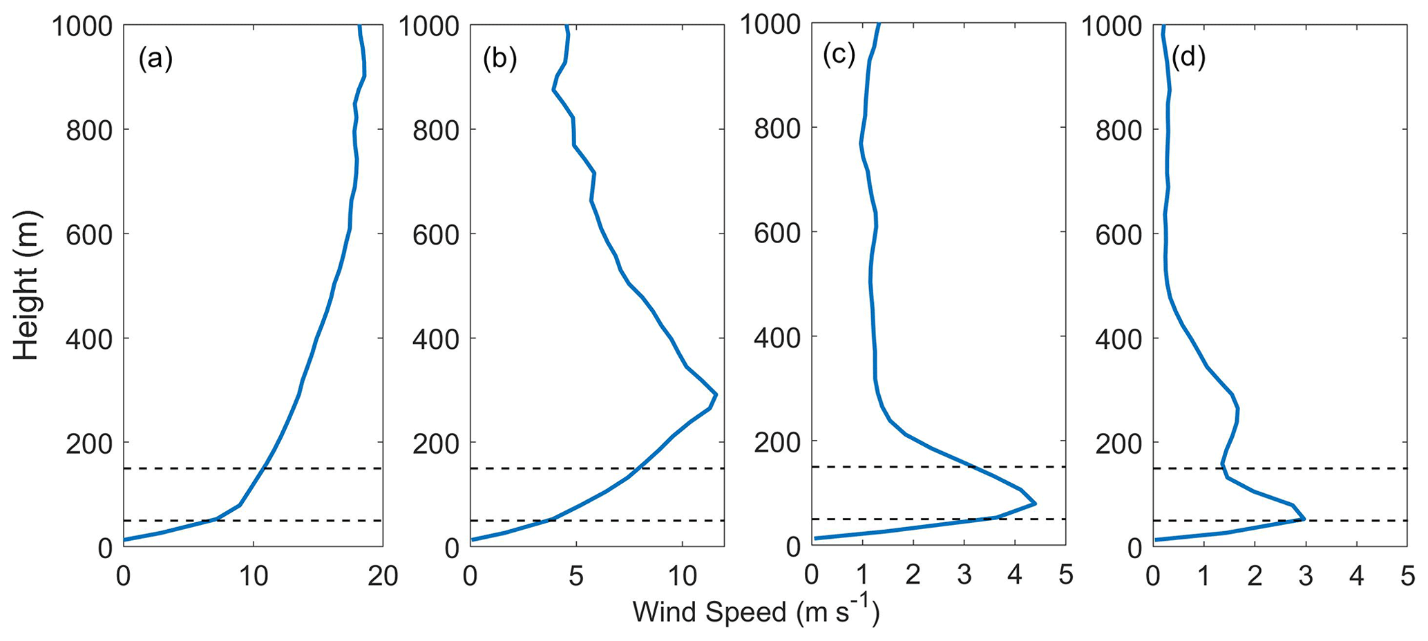
Figure 16Examples of wind profiles with different vertical shears in the horizontal wind speed: (a) strong shear without the presence of a NLLJ, (b) strong shear due to a NLLJ, (c) a NLLJ with the core inside the rotor layer and (d) a NLLJ immediately below the rotor layer. The dashed lines mark the mean rotor layer of 50–150 m a.g.l.
3.2.2 Wind shear and veer through the rotor layer
While NLLJs are beneficial for the nocturnal power generation, their occurrence also has adverse implications for the turbines. Wind shear and veer in the rotor layer, here defined as 50–150 m a.g.l., were considerable during the occurrence of NLLJs, as indicated in the examples of wind profiles with different wind shear values (Fig. 16). These are a case with (a) strong positive shear without the presence of a NLLJ, (b) strong positive shear due to a NLLJ, (c) a NLLJ with the core inside the rotor layer, causing positive shear below and negative shear above the core, and (d) a NLLJ with a core immediately below the rotor layer, which leads to negative vertical shear in the entire rotor layer. It is important to mention that when the NLLJ core falls within the rotor layer, care should be taken of how the shear, and thus the mechanical loading, is calculated. If we were to calculate the mean shear taking positive and negative shear together, it would result in a false impression of small shear. We therefore calculated the shear based on absolute values across the rotor layer for these conditions.
The shear was substantially larger during NLLJs events. The mean wind shear in the mean rotor layer (50–150 m) had an increase of about 67 % during NLLJ events. A similar value was found for V112 since that turbine type has a similar rotor layer (38–150 m). The higher E-126 (71.5–198.5 m) had a mean shear 53 % lower, but the increase during NLLJs was 84 %. We rarely saw negative shear values from cases like those illustrated in Fig. 16d, and those that occurred were often below the cut-in wind speed, consistent with having relatively few and weak NLLJs at very low levels.
Our results indicate that almost half (48 %) of all cases with extreme wind shear coincide with NLLJs (Fig. 17a). It implies that NLLJs are as important as storms for causing strong wind shear. Out of all occurring NLLJs, 37 % of NLLJs lead to extreme shear through the rotor layer. We here defined extreme wind shear through the rotor layer as the 90 % percentile, following Debnath et al. (2021), which corresponded to a similar threshold of 0.0354 s−1. The extreme shear was primarily explained by larger core wind speeds for NLLJs at similar heights rather than stronger NLLJs at higher altitudes. This can be seen by the similar distributions of the NLLJ height paired with a shift in the distribution of core wind speeds during NLLJs with extreme shear (Fig. 17b and c).
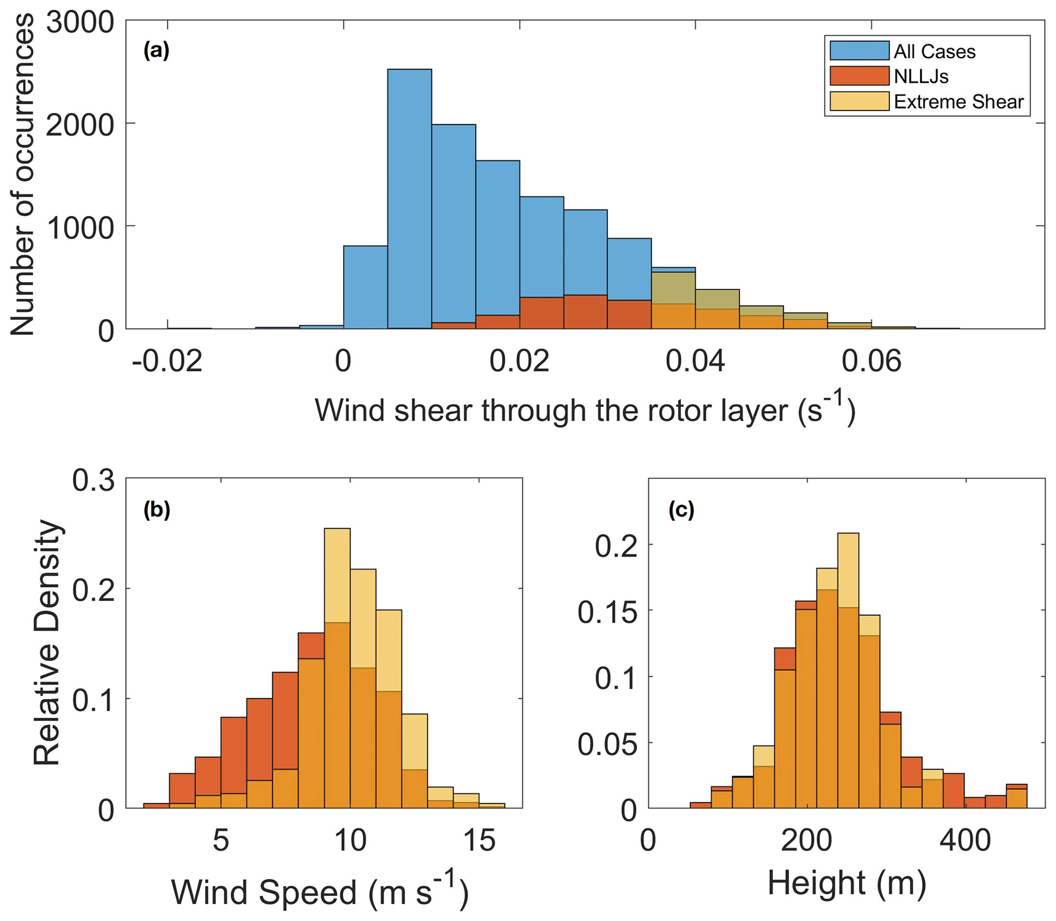
Figure 17Vertical shear of wind speed in the rotor layer. Shown are (a) the number of occurrences of vertical shear in the rotor layer and the frequency of (b) wind speed and (c) height. All conditions are shown in blue, NLLJs in red and extreme shear cases in yellow. Extreme shear was defined by the 90 % percentile (0.0354 s−1).
In addition to shear, the wind veer with height across the rotor layer also has implications for the mechanical loading on the rotors. We therefore quantified the absolute wind veer across the rotor layer during NLLJ events (Fig. 18). The magnitude of the wind veer was typically larger during NLLJ events with a mean of 0.174∘ m−1 against 0.145∘ m−1 during all cases. It corresponded to a mean increase in the veer by about 20 %. The results for V112 were similar and slight differences were seen for E-126. For E-126, the average veer was 11 % lower than for V112 and the mean increase was 12 % during NLLJs.
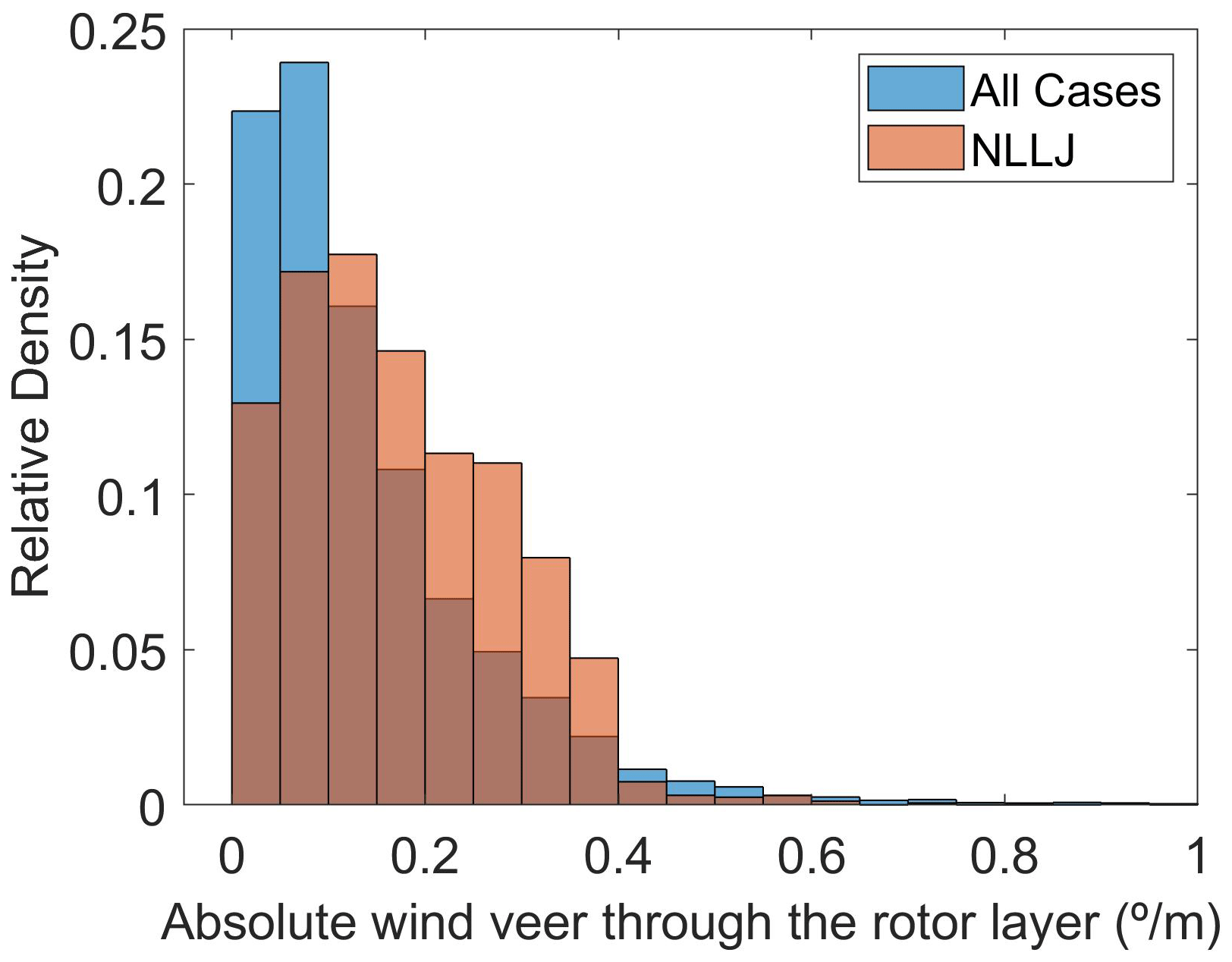
Figure 18Wind veer in the rotor layer. Shown is the frequency of the absolute wind veer in the mean rotor layer (50–150 m a.g.l.) during all nights (blue) and during NLLJs (red).
NLLJs have positive and negative impacts on wind turbines. The wind power production clearly benefits from NLLJ occurrences, and this positive impact increases with the height of the turbine. At the same time, the wind shear and veer during NLLJs also increase with the height a.g.l. Shear and veer can affect both the structure of the turbines and also the expected power output to different values from the power curves (Murphy et al., 2020). These results indicate that installing higher turbines that are able to benefit from this higher wind speed and are sufficiently stable to sustain high shear and veer would be ideal for increasing the wind power production during stable stratification of the near-surface boundary layer. In addition, due to the changes in the expected power output, it is clear that ignoring the shear in the rotor layer and only measuring wind at the hub height would affect wind power estimates. Another important effect is that the NLLJ wind profiles are very different from the often assumed logarithmic or power-law profiles used to extrapolate winds from 10 m to hub heights (Gualtieri, 2019; Hallgren et al., 2020). These approximations can lead to large errors in estimates of wind power potential, especially during NLLJs when the vertical wind profile strongly differs from average conditions. This is a particular problem for wind power estimates in locations with frequent occurrences of NLLJs.
Forecasts and reanalysis data do not fully characterize NLLJs with a sufficient accuracy. Monitoring vertical profiles of winds and temperature for site assessments is therefore important for planning new wind power installations. In this context, accurate representations of NLLJs in atmospheric models is of great importance for grid planning and power forecasting. Our results shows that synoptic-scale weather patterns over all Europe are no clear indication for NLLJ occurrence since most patterns could be associated with a NLLJ. Statistically, however, anticyclonic weather patterns stood out as favoring NLLJ developments. These included weather patterns that can be connected to atmospheric blocking events. Atmospheric models are known to have difficulties in representing the correct onset and decay of such events (Tibaldi and Molteni, 1990; Lupo, 2021), which needs to be resolved in the future for better wind power forecasts. Studies about NLLJs with high temporal and spatial resolution are useful to the extent that they help one to better understand their driving mechanisms including the evolution of boundary layer characteristics and the influence of meso- to synoptic-scale weather developments. The present study is one step in that direction, but more can be done to support the energy transition using more wind power. Other techniques, including machine learning, may be important tools to understand their large-scale driving mechanisms. One such aspect is the extent to which NLLJs change with global warming, which is currently not understood but important for the operation of a future energy system.
This paper analyzes the spatiotemporal characteristics of nocturnal low-level jets (NLLJ) from June to August 2020, during the FESST@home campaign, at two sites in eastern Germany: Falkenberg and Lindenberg. In addition, the impact of NLLJs on wind power production is quantified. NLLJs occurred in 64 % and 73 % of the nights, depending on the site. About half of them had lifetimes exceeding 3 h. The differences between both sites may depend on the different local characteristics (e.g., terrain) and, to a lesser extent, on the different operation modes of the lidars.
Detailed analyses of the NLLJs at the two sites also suggested different driving mechanisms for their development. Very long NLLJs occurred more often simultaneously at both sites, indicating their mesoscale character. In our work, at least in the sub-class meso-gama (2–20 km). Our results suggest that NLLJs with long lifetimes are driven by inertial oscillations perturbed by nocturnal changes in the synoptic-scale horizontal pressure gradient and intermittent turbulent mixing. This was further supported by the prevailing synoptic weather patterns for long NLLJs. Many long NLLJs occurred during anticyclonic weather patterns as one would expect would be favorable for inertial oscillations. These results agree with the classical theory on inertial oscillation linking NLLJ development to stable atmospheric conditions and horizontal pressure gradients in the mesoscale (Stensrud, 1996; Beyrich et al., 1997; Salio et al., 2007).
Shorter NLLJ events are more strongly affected by local conditions. For instance, short NLLJs occurred more frequently in Lindenberg, suggesting stronger local influences on the NLLJ development than in Falkenberg. Short NLLJs can be caused by an earlier breakdown of a NLLJ development or be driven by other meteorological processes, such as jet profiles created by frontal passages or density currents from convective downdrafts. This was again consistent with the prevailing cyclonic weather synoptic-scale weather patterns for short NLLJs. However, it is clear from our analysis that the synoptic-weather pattern alone is no clear indicator for whether a NLLJ forms or not.
NLLJs can have both beneficial and adverse impacts on wind power production. NLLJs increased the nocturnal power generation but also increased wind speed and directional shear across the rotor layer. During the campaign, about 25 % of the power production was generated during NLLJ conditions. The magnitude of the effects depended on the hub height of the turbine. We estimated a wind power production increase by 50 % (80 %) for hub heights of 94 (135) m a.g.l. during NLLJs. Out of all NLLJs, 37 % lead to extreme wind speed shear across the rotor layer. Compared to all extreme shear cases, 48 % were caused by NLLJs. It highlights the strong impact of NLLJs for generating low-level shear during summer in Germany. These results imply that power production with higher turbines would more strongly benefit from NLLJs, particularly when the adverse effect of wind shear and veer from the NLLJs is considered in the turbine construction.
Taken together, long NLLJs driven by perturbed inertial oscillations have a greater importance for wind power production. Long events not only sustained high wind speeds in the rotor layer over a longer time period but also had a mesoscale spatial extension, holding the potential to affect one or several wind parks at the same time. In contrast, short NLLJs were often more local and did not as often affect different sites simultaneously. Short NLLJs are therefore expected to cause power ramps, i.e., fast increases and decreases in power production, increasing the spatiotemporal variability in power production. Future work will address the meteorological processes of NLLJs with longer datasets and for larger regions including offshore regions and complex terrain.
The Doppler lidar data are available from https://doi.org/10.25592/UHHFDM.9758 (Steinheuer et al., 2021).
EWL was responsible for the conceptualization and writing of the original draft. The data validation, methodology and coding were also part of the author's contribution. SF supervised the paper's content conceptualization while also helping with the review and editing, as well as the methodology development.
The contact author has declared that neither of the authors has any competing interests.
Publisher's note: Copernicus Publications remains neutral with regard to jurisdictional claims in published maps and institutional affiliations.
This work was carried out in the framework of the Hans-Ertel-Centre for Weather Research. We thank the instrument operators for carrying out the measurements during FESST@home, as well as the German Weather Service and Julian Steinheuer for providing the Doppler lidar wind data. We also thank Paul James for providing the Großwetterlage weather pattern data used in this work.
This research has been supported by the Hans-Ertel-Centre for Weather Research, “Climate Monitoring and Diagnostic” (grant no. BMVI/DWD 4818DWDP5A).
This paper was edited by Rebecca Barthelmie and reviewed by Fernando Martins and one anonymous referee.
Abkar, M., Sharifi, A., and Porté-Agel, F.: Wake flow in a wind farm during a diurnal cycle, J. Turbulence, 17, 420–441, https://doi.org/10.1080/14685248.2015.1127379, 2016. a
Aird, J. A., Barthelmie, R. J., Shepherd, T. J., and Pryor, S. C.: WRF-simulated low-level jets over Iowa: characterization and sensitivity studies, Wind Energ. Sci., 6, 1015–1030, https://doi.org/10.5194/wes-6-1015-2021, 2021. a, b
Andreas, E. L., Claffy, K. J., and Makshtas, A. P.: Low-Level Atmospheric Jets And Inversions Over The Western Weddell Sea, Bound.-Lay. Meteorol., 97, 459–486, https://doi.org/10.1023/A:1002793831076, 2000. a
Baas, P., Bosveld, F. C., Baltink, H. K., and Holtslag, A. A.: A climatology of nocturnal low-level jets at Cabauw, J. Appl. Meteorol. Clim., 48, 1627–1642, https://doi.org/10.1175/2009JAMC1965.1, 2009. a, b
Banta, R., Newsom, R. K., Lundquist, J. K., Pichugina, Y. L., Coulter, R. L., and Mahrt, L.: Nocturnal Low-Level Jet Characteristics Over Kansas During Cases-99, Bound.-Lay. Meteorol., 105, 221–252, https://doi.org/10.1023/A:1019992330866, 2002. a, b
Beyrich, F.: Sodar observations of the stable boundary layer height in relation to the nocturnal low-level jet, Meteorol. Z., 3, 29–34, 1994. a
Beyrich, F., Kalass, D., and Weisensee, U.: Influence of the nocturnal low-level-jet on the vertical and mesoscale structure of the stable boundary layer as revealed from doppler-sodar-observations, in: Acoustic remote sensing applications, Springer, 236–246, https://doi.org/10.1007/BFb0009568, 1997. a, b, c
Blackadar, A. K.: Boundary Layer Wind Maxima and Their Significance for the Growth of Nocturnal Inversions, B. Am. Meteorol. Soc., 38, 283–290, https://doi.org/10.1175/1520-0477-38.5.283, 1957. a, b, c
Brown, A., Beljaars, A., Hersbach, H., Hollingsworth, A., Miller, M., and Vasiljevic, D.: Wind turning across the marine atmospheric boundary layer, Q. J. Roy. Meteorol. Soc., 131, 1233–1250, 2005. a
Brown, A., Beare, R., Edwards, J., Lock, A., Keogh, S., Milton, S., and Walters, D.: Upgrades to the boundary-layer scheme in the Met Office numerical weather prediction model, Bound.-Lay. Meteorol., 128, 117–132, 2008. a
Debnath, M., Doubrawa, P., Optis, M., Hawbecker, P., and Bodini, N.: Extreme wind shear events in US offshore wind energy areas and the role of induced stratification, Wind Energ. Sci., 6, 1043–1059, https://doi.org/10.5194/wes-6-1043-2021, 2021. a
Doosttalab, A., Siguenza-Alvarado, D., Pulletikurthi, V., Jin, Y., Bocanegra Evans, H., Chamorro, L. P., and Castillo, L.: Interaction of low-level jets with wind turbines: On the basic mechanisms for enhanced performance, J. Renew. Sustain. Energ., 12, 053301, https://doi.org/10.1063/5.0017230, 2020. a
Druecke, J., Borsche, M., James, P., Kaspar, F., Pfeifroth, U., Ahrens, B., and Trentmann, J.: Climatological analysis of solar and wind energy in Germany using the Grosswetterlagen classification, Renew. Energy, 164, 1254–1266, https://doi.org/10.1016/j.renene.2020.10.102, 2021. a
Emeis, S.: Wind speed and shear associated with low-level jets over Northern Germany, Meteorol. Z., 23, 295–304, https://doi.org/10.1127/0941-2948/2014/0551, 2014. a, b, c, d
Englberger, A., Lundquist, J. K., and Dörnbrack, A.: Changing the rotational direction of a wind turbine under veering inflow: a parameter study, Wind Energ. Sci., 5, 1623–1644, https://doi.org/10.5194/wes-5-1623-2020, 2020. a
FESSTVal: FESSTVaL – Field Experiment on Submesoscale Spatio-Temporal Variability in Lindenberg, https://fesstval.de/en/ (last access: 18 July 2022), 2020. a
Fiedler, S., Schepanski, K., Heinold, B., Knippertz, P., and Tegen, I.: Climatology of nocturnal low-level jets over North Africa and implications for modeling mineral dust emission, J. Geophys. Res.-Atmos., 118, 6100–6121, 2013. a, b
Frank, C., Fiedler, S., and Crewell, S.: Balancing potential of natural variability and extremes in photovoltaic and wind energy production for European countries, Renew. Energy, 163, 674–684, 2021. a
Gualtieri, G.: A comprehensive review on wind resource extrapolation models applied in wind energy, Renew. Sustain. Energ. Rev., 102, 215–233, 2019. a
Gutierrez, W., Araya, G., Kiliyanpilakkil, P., Ruiz-Columbie, A., Tutkun, M., and Castillo, L.: Structural impact assessment of low level jets over wind turbines, J. Renew. Sustain. Energ., 8, 023308, https://doi.org/10.1063/1.4945359, 2016. a, b, c
Gutierrez, W., Ruiz-Columbie, A., Tutkun, M., and Castillo, L.: Impacts of the low-level jet's negative wind shear on the wind turbine, Wind Energ. Sci., 2, 533–545, https://doi.org/10.5194/wes-2-533-2017, 2017. a
Hallgren, C., Arnqvist, J., Ivanell, S., Körnich, H., Vakkari, V., and Sahlée, E.: Looking for an offshore low-level jet champion among recent reanalyses: a tight race over the Baltic Sea, Energies, 13, 3670 https://doi.org/10.3390/en13143670, 2020. a, b, c, d, e
Han, Y., Yang, Q., Liu, N., Zhang, K., Qing, C., Li, X., Wu, X., and Luo, T.: Analysis of wind-speed profiles and optical turbulence above Gaomeigu and the Tibetan Plateau using ERA5 data, Mon. Notic. Roy. Astron. Soc., 501, 4692–4702, https://doi.org/10.1093/mnras/staa2960, 2021. a
Heinold, B., Knippertz, P., Marsham, J., Fiedler, S., Dixon, N., Schepanski, K., Laurent, B., and Tegen, I.: The role of deep convection and nocturnal low-level jets for dust emission in summertime West Africa: Estimates from convection-permitting simulations, J. Geophys. Res.-Atmos., 118, 4385–4400, 2013. a
Hersbach, H., Bell, B., Berrisford, P., Hirahara, S., Horányi, A., Muñoz-Sabater, J., Nicolas, J., Peubey, C., Radu, R., Schepers, D., Simmons, A., Soci, C., Abdalla, S., Abellan, X., Balsamo, G., Bechtold, P., Biavati, G., Bidlot, J., Bonavita, M., Chiara, G., Dahlgren, P., Dee, D., Diamantakis, M., Dragani, R., Flemming, J., Forbes, R., Fuentes, M., Geer, A., Haimberger, L., Healy, S., Hogan, R. J., Hólm, E., Janisková, M., Keeley, S., Laloyaux, P., Lopez, P., Lupu, C., Radnoti, G., Rosnay, P., Rozum, I., Vamborg, F., Villaume, S., and Thépaut, J.: The ERA5 global reanalysis, Q. J. Roy. Meteorol. Soc., 146, 1999–2049, 2020. a, b
IRENA: Future of wind: Deployment, investment, technology, grid integration and socio-economic aspects (A Global Energy Transformation paper), Tech. rep., International Renewable Energy Agency, Abu Dhabi, https://www.irena.org/publications/2019/Oct/Future-of-wind (last access: 18 July 2022), 2019. a
James, P.: An objective classification method for Hess and Brezowsky Grosswetterlagen over Europe, Theor. Appl. Climatol., 88, 17–42, 2007. a, b, c
Kalverla, P. C., Duncan, J. B., Steeneveld, G. J., and Holtslag, A. A.: Low-level jets over the north sea based on ERA5 and observations: Together they do better, Wind Energ. Sci., 4, 193–209, https://doi.org/10.5194/wes-4-193-2019, 2019. a, b
Lampert, A., Bernalte Jimenez, B., Gross, G., Wulff, D., and Kenull, T.: One-year observations of the wind distribution and low-level jet occurrence at Braunschweig, North German Plain, Wind Energy, 19, 1807–1817, https://doi.org/10.1002/we.1951, 2016. a
Lupo, A. R.: Atmospheric blocking events: a review, Ann. NY. Acad. Sci., 1504, 5–24, 2021. a
Marke, T., Crewell, S., Schemann, V., Schween, J. H., and Tuononen, M.: Long-term observations and high-resolution modeling of midlatitude nocturnal boundary layer processes connected to low-level jets, J. Appl. Meteorol. Clim., 57, 1155–1170, https://doi.org/10.1175/JAMC-D-17-0341.1, 2018. a
Mirocha, J. D., Simpson, M. D., Fast, J. D., Berg, L. K., and Baskett, R. L.: Investigation of boundary-layer wind predictions during nocturnal low-level jet events using the Weather Research and Forecasting model, Wind Energy, 19, 739–762, https://doi.org/10.1002/we.1862, 2016. a
Murphy, P., Lundquist, J. K., and Fleming, P.: How wind speed shear and directional veer affect the power production of a megawatt-scale operational wind turbine, Wind Energ. Sci., 5, 1169–1190, https://doi.org/10.5194/wes-5-1169-2020, 2020. a, b
OECD/IEA: International Energy Agency (IEA), World Energy Outlook 2017, Tech. rep., OECD/IEA, https://www.iea.org/reports/world-energy-outlook-2017 (last access: 18 July 2022), 2017. a, b
Päschke, E., Leinweber, R., and Lehmann, V.: An assessment of the performance of a 1.5 µm Doppler lidar for operational vertical wind profiling based on a 1-year trial, Atmos. Meas. Tech., 8, 2251–2266, https://doi.org/10.5194/amt-8-2251-2015, 2015. a
Pearson, G., Davies, F., and Collier, C.: An Analysis of the Performance of the UFAM Pulsed Doppler Lidar for Observing the Boundary Layer, J. Atmos. Ocean. Tech., 26, 240–250, https://doi.org/10.1175/2008JTECHA1128.1, 2009. a
Peña Diaz, A., Mikkelsen, T., Gryning, S.-E., Hasager, C. B., Hahmann, A. N., Badger, M., Karagali, I., and Courtney, M.: Offshore vertical wind shear: Final report on NORSEWInD's work task 3.1, Tech. rep., DTU Wind Energy, https://orbit.dtu.dk/en/publications/offshore-vertical-wind-shear-final-report-on-norsewinds-work-task (last access: 18 July 2022), 2012. a
Pichugina, Y. L., Brewer, W. A., Banta, R. M., Choukulkar, A., Clack, C. T. M., Marquis, M. C., McCarty, B. J., Weickmann, A. M., Sandberg, S. P., Marchbanks, R. D., and Hardesty, R. M.: Properties of the offshore low level jet and rotor layer wind shear as measured by scanning Doppler Lidar, Wind Energy, 20, 987–1002, https://doi.org/10.1002/we.2075, 2017. a, b
Rohrig, K., Berkhout, V., Callies, D., Durstewitz, M., Faulstich, S., Hahn, B., Jung, M., Pauscher, L., Seibel, A., Shan, M., Siefert, M., Steffen, J., Collmann, M., Czichon, S., Dörenkämper, M., Gottschall, J., Lange, B., Ruhle, A., Sayer, F., Stoevesandt, B., and Wenske, J.: Powering the 21st century by wind energy – Options, facts, figures, Appl. Phys. Rev., 6, 031303, https://doi.org/10.1063/1.5089877, 2019. a, b
Sadorsky, P.: Wind energy for sustainable development: Driving factors and future outlook, J. Clean. Product., 289, 125779, https://doi.org/10.1016/j.jclepro.2020.125779, 2021. a
Salio, P., Nicolini, M., and Zipser, E. J.: Mesoscale convective systems over southeastern South America and their relationship with the South American low-level jet, Mon. Weather Rev., 135, 1290–1309, 2007. a, b
Sandu, I., Beljaars, A., Bechtold, P., Mauritsen, T., and Balsamo, G.: Why is it so difficult to represent stably stratified conditions in numerical weather prediction (NWP) models?, J. Adv. Model. Earth Syst., 5, 117–133, 2013. a, b
Shapiro, A. and Fedorovich, E.: Analytical description of a nocturnal low-level jet, Q. J. Roy. Meteorol. Soc., 136, 1255–1262, https://doi.org/10.1002/qj.628, 2010. a, b
Sharma, V., Parlange, M. B., and Calaf, M.: Perturbations to the Spatial and Temporal Characteristics of the Diurnally-Varying Atmospheric Boundary Layer Due to an Extensive Wind Farm, Bound.-Lay. Meteorol., 162, 255–282, https://doi.org/10.1007/s10546-016-0195-0, 2017. a
Sisterson, D. L. and Frenzen, P.: Nocturnal boundary-layer wind maxima and the problem of wind power assessment, Environ. Sci. Technol., 12, 218–221, https://doi.org/10.1021/es60138a014, 1978. a
Smalikho, I. N. and Banakh, V. A.: Measurements of wind turbulence parameters by a conically scanning coherent Doppler lidar in the atmospheric boundary layer, Atmos. Meas. Tech., 10, 4191–4208, https://doi.org/10.5194/amt-10-4191-2017, 2017. a
Steinheuer, J., Detring, C., Kayser, M., and Leinweber, R.: Doppler wind lidar wind and gust data from FESTVAL 2019/2020, Falkenberg, data version 01, Universität Hamburg [data set], https://doi.org/10.25592/UHHFDM.9758, 2021. a
Steinheuer, J., Detring, C., Beyrich, F., Löhnert, U., Friederichs, P., and Fiedler, S.: A new scanning scheme and flexible retrieval for mean winds and gusts from Doppler lidar measurements, Atmos. Meas. Tech., 15, 3243–3260, https://doi.org/10.5194/amt-15-3243-2022, 2022. a
Stensrud, D. J.: Importance of low-level jets to climate: A review, J. Climate, 9, 1698–1711, https://doi.org/10.1175/1520-0442(1996)009<1698:IOLLJT>2.0.CO;2, 1996. a
Suomi, I., Gryning, S. E., O'Connor, E. J., and Vihma, T.: Methodology for obtaining wind gusts using Doppler lidar, Q. J. Roy. Meteorol. Soc., 143, 2061–2072, https://doi.org/10.1002/qj.3059, 2017. a, b
Svensson, G. and Holtslag, A. A.: Analysis of model results for the turning of the wind and related momentum fluxes in the stable boundary layer, Bound.-Lay. Meteorol., 132, 261–277, 2009. a
Svensson, N., Bergström, H., Rutgersson, A., and Sahlée, E.: Modification of the Baltic Sea wind field by land‐sea interaction, Wind Energy, 22, 764–779, https://doi.org/10.1002/we.2320, 2019. a
Tibaldi, S. and Molteni, F.: On the operational predictability of blocking, Tellus A, 42, 343–365, 1990. a
Tuononen, M., O'Connor, E. J., Sinclair, V. A., and Vakkari, V.: Low-level jets over Utö, Finland, based on Doppler lidar observations, J. Appl. Meteorol. Clim., 56, 2577–2594, 2017. a
Vanderwende, B. J. and Lundquist, J. K.: The modification of wind turbine performance by statistically distinct atmospheric regimes, Environ. Res. Lett., 7, 034035, https://doi.org/10.1088/1748-9326/7/3/034035, 2012. a
Van de Wiel, B. J. H., Moene, A. F., Steeneveld, G. J., Baas, P., Bosveld, F. C., and Holtslag, A. A. M.: A Conceptual View on Inertial Oscillations and Nocturnal Low-Level Jets, J. Atmos. Sci., 67, 2679–2689, https://doi.org/10.1175/2010JAS3289.1, 2010. a, b, c
Wagner, D., Steinfeld, G., Witha, B., Wurps, H., and Reuder, J.: Low level jets over the southern North Sea, Meteorol. Z., 28, 389–415, https://doi.org/10.1127/metz/2019/0948, 2019. a
Wharton, S. and Lundquist, J. K.: Atmospheric stability affects wind turbine power collection, Environ. Res. Lett., 7, 014005, https://doi.org/10.1088/1748-9326/7/1/014005, 2012. a
Ziemann, A., Galvez Arboleda, A., and Lampert, A.: Comparison of Wind Lidar Data and Numerical Simulations of the Low-Level Jet at a Grassland Site, Energies, 13, 6264, https://doi.org/10.3390/en13236264, 2020. a, b, c, d, e, f