Turbulence in a coastal environment: the case of Vindeby

The one-point and two-point power spectral densities of the wind velocity fluctuations are studied using the observations from an offshore mast at Vindeby Offshore Wind Farm, for a wide range of thermal stratifications of the atmosphere. A comparison with estimates from the FINO1 platform (North Sea) is made to identify shared spectral characteristics of turbulence between different offshore sites. The sonic anemometer measurement data at 6, 18, and 45 m a.m.s.l. (above mean sea level) are considered. These heights are lower than at the FINO1 platform, where the measurements were collected at heights between 40 and 80 m. Although the sonic anemometers are affected by transducer-flow distortion, the spectra of the along-wind velocity component are consistent with those from FINO1 when surface-layer scaling is used, for near-neutral and moderately diabatic conditions. The co-coherence of the along-wind component, estimated for vertical separations under near-neutral conditions, matches remarkably well with the results from the dataset at the FINO1 platform. These findings mark an important step toward more comprehensive coherence models for wind load calculation. The turbulence characteristics estimated from the present dataset are valuable for better understanding the structure of turbulence in the marine atmospheric boundary layer and are relevant for load estimations of offshore wind turbines. Yet, the datasets recorded at Vindeby and FINO1 cover only the lower part of the rotor of state-of-the-art offshore wind turbines. Further improvements in the characterisation of atmospheric turbulence for wind turbine design will require measurements at heights above 100 m a.m.s.l.

1 Introduction

In the early 1990s, the first generations of offshore wind farms were commissioned to test the viability of extracting wind power in the marine atmospheric boundary layer (MABL). The first was Vindeby Offshore Wind Farm, which provided electricity to around 2200 homes during its 25 years of operation, with a total generated power of 243 GW h (Power Technology, 2020). The project was deemed successful and marked the beginning of the offshore wind sector.

Not only was the Vindeby project the first offshore wind farm, but also it provided precious information on meteorological conditions in the MABL using offshore and onshore meteorological masts. The data collected have been used to study the characteristics of the mean wind speed profile under various atmospheric conditions (Barthelmie et al., 1994; Barthelmie, 1999). The masts were also instrumented with 3D sonic anemometers to study turbulence, but these data were used in a limited number of studies only (e.g.  Mahrt et al., 1996, 2001).

The characteristics of the MABL differ from the overland atmospheric boundary layer (ABL) due to the large proportion of non-neutral atmospheric stability conditions (Barthelmie, 1999; Archer et al., 2016) and low roughness lengths. Since the 2010s, several studies have indicated that diabatic wind conditions may significantly affect the fatigue life of offshore wind turbine (OWT) components (Sathe et al., 2013; Hansen et al., 2014; Holtslag et al., 2016; Doubrawa et al., 2019; Nybø et al., 2020; Putri et al., 2020). Recent measurements from the first commercial floating wind farm (Hywind Scotland) have even shown the direct influence of atmospheric stability on the floater motions (Jacobsen and Godvik, 2021). Diabatic conditions are more likely to affect floating wind turbines than bottom-fixed ones as the first few eigenfrequencies of large floating wind turbines are close to or below 0.02 Hz (Nielsen et al., 2006), which is the frequency range mainly affected by the thermal stratification of the atmosphere. To model properly the wind load for wind turbine design, a better understanding of the spectral structure of turbulence in the MABL is necessary, which addresses partly the first of the three great challenges in the field of wind energy (Veers et al., 2019).

The limitations of current guidelines for offshore turbulence modelling, such as IEC 61400-1 (2005), have been highlighted in the past (Cheynet et al., 2017, 2018). Site-specific measurements advised by IEC 61400-1 (2005) are related to the mean flow and integral turbulence characteristics. However, for the spectral characteristics, appropriate scaling can be used to display universal shapes over specific frequency ranges. In this regard, the present study addresses similar challenges to those discussed by Kelly (2018) but focuses on some specific aspects not covered by the spectral tensor of homogeneous turbulence (Mann, 1994). Firstly, the low-frequency fluctuations are generally underestimated by the uniform-shear model, especially under convective conditions (De Maré and Mann, 2014; Chougule et al., 2018). Secondly, the version of the uniform-shear model (Mann, 1994) used within the field of wind energy does not account for the blocking by the ground, which may lead to an overestimation of the co-coherence of both the along-wind and the vertical wind components for near-neutral conditions (Cheynet, 2019). Thus, the co-coherence modelling using the uniform-shear model (Mann, 1994) is not discussed further in the present study.

Using the unexplored sonic anemometer data from the Vindeby database, this study looks at the characteristics of offshore turbulence in the frequency space. The objective is to quantify the similarities between these characteristics and those identified at FINO1 (Cheynet et al., 2018). Such a comparison is relevant to establishing new offshore wind turbulence models that can be used to improve the design of future multi-megawatt offshore wind turbines. Whereas the measurement data from FINO1 were obtained 40 km away from the shore, at heights between 40 m and 80 m a.m.s.l. (above mean sea level), those from the Vindeby database were collected only 3 km from the coast and at heights between 6 m and 45 m a.m.s.l. Therefore, the two datasets offer a complementary description of wind turbulence above the sea.

The present study is organised as follows: Sect. 2 describes the instrumentation and the site topography. Section 3 summarises the data processing, the assumptions, and the models used to study the spectral characteristics of turbulence. Section 4 presents the methodology used to assess the data quality and selection of stationary velocity data. Section 5 first evaluates the applicability of surface-layer scaling for the anemometer records at 6 m a.m.s.l. Then, the one-point velocity spectra and co-coherence estimates from Vindeby are compared with predictions from semi-empirical models which are based on FINO1 observations (Cheynet et al., 2018) to assess the similarities of the spectral characteristics between the two sites. Finally, the applicability of the Vindeby database to the design of an adequate turbulence model for offshore wind turbines is discussed in Sect. 5.5.

2 Instrumentation and site description

Vindeby Offshore Wind Farm operated in Denmark from 1991 to 2016 and was decommissioned in 2017. It was located 1.5 to 3 km from the northwestern coast of the island of Lolland (Fig. 1). Due to its location, Vindeby may be regarded as a coastal site instead of an offshore one. Vindeby has a flat topography with an average elevation of under 11 m a.m.s.l., whereas the water depth around the wind farm ranges from 2 to 5 m (Barthelmie et al., 1994). As pointed out by Johnson et al. (1998), the average significant wave height H_s at Vindeby is under 1 m. The water depth increases from around 3 m in the proximity of the wind farm up to approximately 20 m away from the northern side of the wind farm.

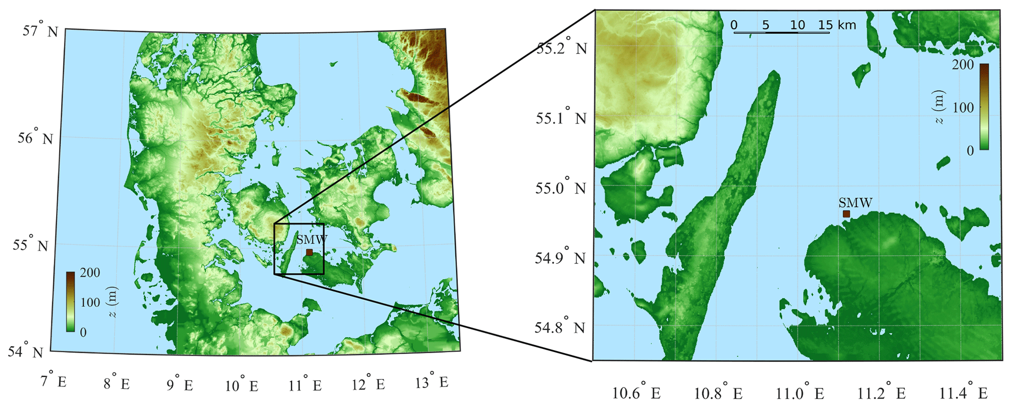
Figure 1 Digital elevation model of southern Denmark showing the location of Sea Mast West (SMW), in a sheltered flat coastal environment. Only the wind from 220 to 330^∘ is considered for SMW.

The wind farm comprised 11 Bonus 450 kW turbines arranged in two rows with 300 m spacing along the 325–145^∘ line and three meteorological masts (Fig. 2). The three masts were Land Mast (LM), Sea Mast South (SMS), and Sea Mast West (SMW), and the latter two were placed offshore (Fig. 2). Both SMS and SMW were installed in 1993 and were decommissioned in 2001 and 1998, respectively. Measurements from LM and SMS were used by Barthelmie (1999) to assess the influence of the thermal stratification of the atmosphere on coastal wind climates. The present study considers only wind measurements from SMW due to the availability of the data.

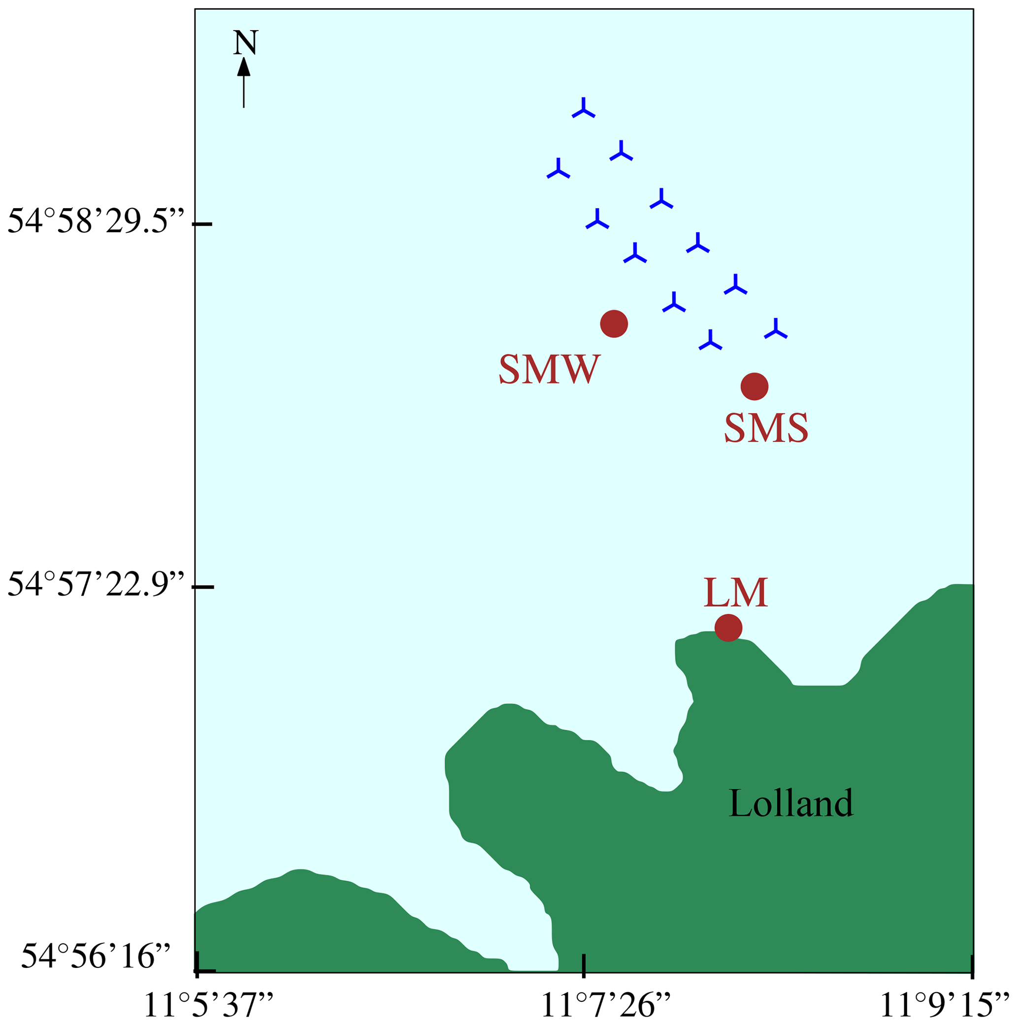
Figure 2 Vindeby Offshore Wind Farm layout with circles marking the position of the masts: SMW, SMS, and LM. SMW is located approximately 1.5 km from Lolland.

SMW was a triangular lattice tower with a height of 48 km a.m.s.l. as sketched in Fig. 3. The booms on the SMW were mounted on both sides of the tower at 46 and 226^∘ from the north and are referred to as the northern and southern boom, respectively. The booms' length ranged from 1.6 to 4 m, and their diameter was 50 mm (Barthelmie et al., 1994). Three F2360a Gill three-axis ultrasonic anemometers (SAs) were mounted on the southern booms at 45, 18, and 6 m a.m.s.l. and operated with a sampling rate of 20 Hz. Two Risø P2021 resolver wind vanes with P2058 wind direction transmitters were located on the northern booms at 43 m and 20 m a.m.s.l. using a sampling frequency of 5 Hz. The height of the vanes' centres above the boom was 600 mm. There were seven cup anemometers mounted on SMW as shown in Fig. 3; however, their measurements were not used here. The air temperature at 10 m a.m.s.l. was recorded using a Risø P2039 PT 100 sensor. The sea surface elevation η was measured using an acoustic wave recorder (AWR) placed on the seabed, 30 m away from SMW, at a depth of 4 m (Johnson et al., 1998). The sea surface elevation data were recorded at a sampling frequency of 8 Hz but stored with a sampling frequency of 20 Hz. The data collected from SMW were transferred to LM using an underwater fibre optic link and stored as time series of 30 min duration. Such a duration is appropriate to study turbulence in coastal and offshore areas (Dobson, 1981). Therefore, the flow characteristics studied herein are based on the averaging time of 30 min.

The fetch around SMW comprises open sea, land, and mixed fetch as shown in Fig. 1. The so-called sea fetch is considered when the wind blows from 220 to 90^∘, with a fetch distance of up to 135 km for the sector ranging from 345 to 355^∘. The direction sectors from 0–50^∘ are those most affected by flow distortion due to the presence of the mast (Barthelmie et al., 1994). Furthermore, the flow from 335–110^∘ might be affected by the wake effects from the wind farm. To exclude the flow disturbed by the presence of the mast and wind turbine wakes and/or internal boundary layers due to roughness changes, only the flow from 220–330^∘ is considered in the present study, which represents 40 % of the velocity data recorded in 1994 and 1995 at SMW. The surface roughness z₀ within the 247-to-292^∘ direction varies with the mean wind speed from 0.00011 to 0.0012 m (Johnson et al., 1998). A more detailed description of the other directional sectors is given by Barthelmie et al. (1994).

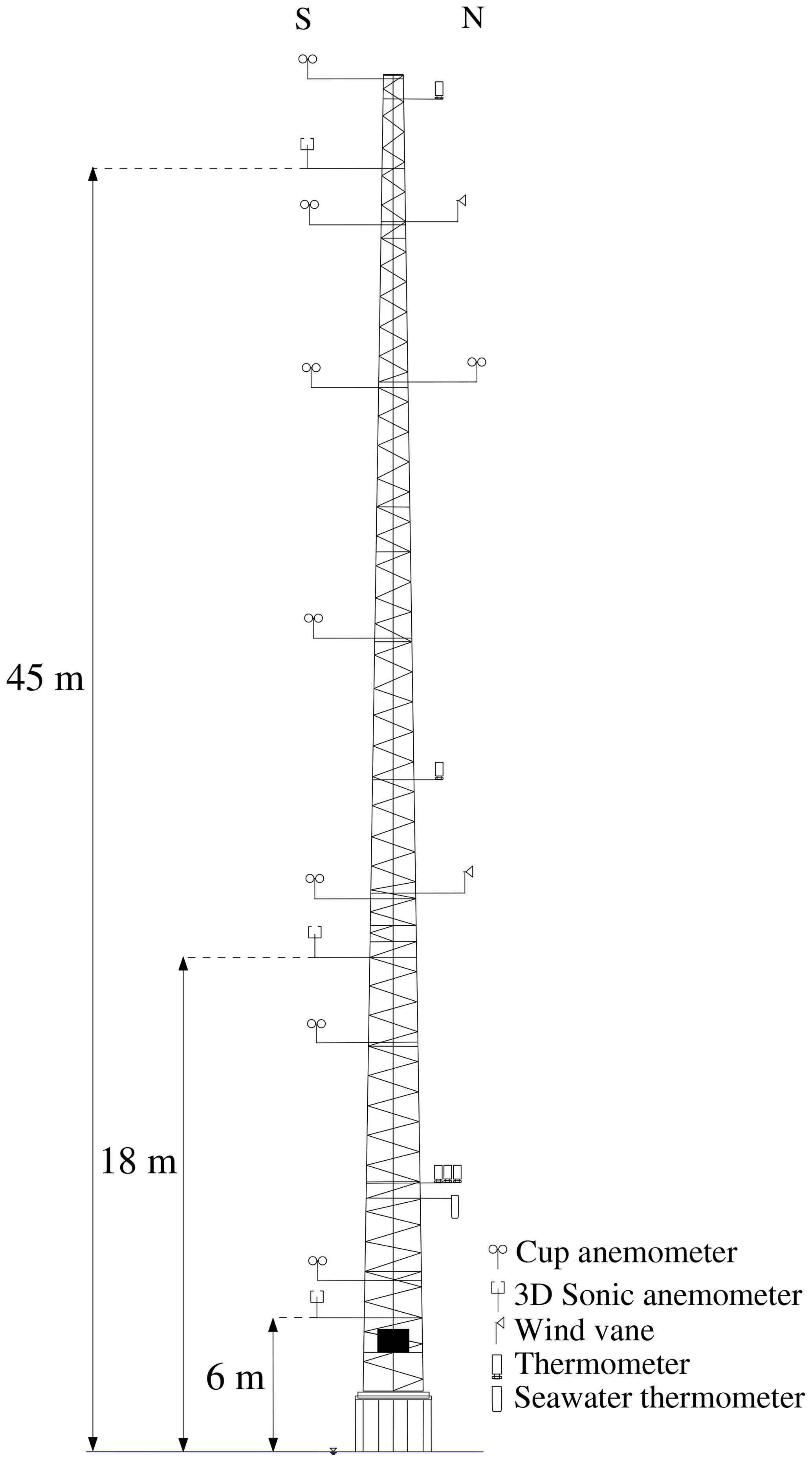
Figure 3 Sketch of the atmospheric instrumentation at SMW. The sonic anemometers are located in the southern boom “S” oriented at 226^∘ from the north.

3 Theoretical background

3.1 Monin–Obukhov theory

The along-wind, cross-wind, and vertical velocity components are denoted as u, v, and w, respectively. Each component is split into a mean ($\stackrel{\mathrm{‾}}{u}$, $\stackrel{\mathrm{‾}}{v}$, $\stackrel{\mathrm{‾}}{w}$) and fluctuating part (u^′, v^′, w^′). In flat and homogeneous terrain, the flow is fairly horizontal; i.e. $\stackrel{\mathrm{‾}}{v}$ and $\stackrel{\mathrm{‾}}{w}$ are approximatively zero. Here, the fluctuating components are assumed to be stationary, Gaussian, ergodic random processes (Monin, 1958).

Although the u component drives the wind turbine's rotor fatigue loads, proper modelling of the v component in terms of power spectral density (PSD) and root coherence may be necessary for skewed flow conditions, which can occur because of a large wind direction shear (Sanchez Gomez and Lundquist, 2020) or wind turbine yaw error (Robertson et al., 2019). To estimate a wind turbine's fatigue loads, the vertical velocity component is likely more relevant in complex terrain than offshore (Mouzakis et al., 1999). Nevertheless, this component is studied here for the sake of completeness. Also, the vertical velocity component provides precious information on the sonic anemometer flow distortion (Cheynet et al., 2019; Peña et al., 2019). The vertical velocity component is also necessary to assess the atmospheric stability using the eddy covariance method and facilitates the study of the waves' influences on the velocity data recorded by the sonic anemometers (e.g. Benilov et al., 1974).

In the atmospheric surface layer, where Monin–Obukhov similarity theory (MOST) generally applies, the scaling velocity is the friction velocity u_*, whereas the scaling lengths are the height z above the surface and the Obukhov length L (Monin and Obukhov, 1954), defined as

$$\begin{array}{}\text{(1)}& L=-{\displaystyle \frac{u_{*}^{\mathrm{3}}{\stackrel{\mathrm{‾}}{\mathit{\theta }}}_{\mathrm{v}}}{g\mathit{\kappa }\left(\stackrel{\mathrm{‾}}{w^{\prime }{\mathit{\theta }}_{\mathrm{v}}^{\prime }}\right)}},\end{array}$$

where ${\stackrel{\mathrm{‾}}{\mathit{\theta }}}_{\mathrm{v}}$ is the mean virtual potential temperature, g=9.81 m s⁻² is the gravitational acceleration, κ≈0.4 is the von Kármán constant (Högström, 1985), and $\stackrel{\mathrm{‾}}{w^{\prime }{\mathit{\theta }}_{\mathrm{v}}^{\prime }}$ is the vertical flux of virtual potential temperature. For a given height z above the surface, the non-dimensional stability parameter $\mathit{\zeta }=z/L$ is used herein to classify the thermal stratification of the atmosphere.

While ${\mathit{\theta }}_{\mathrm{v}}^{\prime }$ can be fairly well approximated by the fluctuating sonic temperature measurement (Schotanus et al., 1983; Sempreviva and Gryning, 1996), the mean value ${\stackrel{\mathrm{‾}}{\mathit{\theta }}}_{\mathrm{v}}$ could not be reliably obtained from the sonic anemometers deployed on SMW (Kurt Hansen, personal communication, 2020). Therefore, ${\stackrel{\mathrm{‾}}{\mathit{\theta }}}_{\mathrm{v}}$ was obtained using the absolute temperature recorded from the Risø P2039 PT 100 sensor at 10 m a.m.s.l., which was converted into the virtual potential temperature using the pressure data from LM and assuming an air relative humidity of 90 % near the sea surface (Stull, 1988). The air pressure data from LM are used due to the absence of air pressure data at SMW and SMS.

Since the covariance between the cross-wind and the vertical component may not be negligible in the MABL (Geernaert, 1988; Geernaert et al., 1993), the friction velocity u_* is computed as suggested by Weber (1999); that is

$$\begin{array}{}\text{(2)}& u_{*}=\sqrt[\mathrm{4}]{{\stackrel{\mathrm{‾}}{u^{\prime }{w}^{\prime }}}^{\mathrm{2}}+{\stackrel{\mathrm{‾}}{v^{\prime }{w}^{\prime }}}^{\mathrm{2}}}.\end{array}$$

A common approach to assess the applicability of MOST is to study the non-dimensional mean wind speed profile ϕ_m defined as

$$\begin{array}{}\text{(3)}& {\mathit{\varphi }}_{\mathrm{m}}\left({\displaystyle \frac{z}{L}}\right)={\displaystyle \frac{\mathit{\kappa }z}{u_{*}}}{\displaystyle \frac{\partial \stackrel{\mathrm{‾}}{u}}{\partial z}}\end{array}$$

as a function of the atmospheric stability (Kaimal and Finnigan, 1994). In the following, ϕ_m is empirically modelled as by Högström (1988):

$$\begin{array}{}\text{(4)}& {\mathit{\varphi }}_{\mathrm{m}}\approx \left\{\begin{array}{ll}(\mathrm{1}+\mathrm{15.2}|\mathit{\zeta }|{)}^{-\mathrm{1}/\mathrm{4}},& -\mathrm{2}\le \mathit{\zeta }<\mathrm{0},\\ \mathrm{1}+\mathrm{4.8}\left(\mathit{\zeta }\right),& \mathrm{0}\le \mathit{\zeta }\le \mathrm{1}.\end{array}\right.\end{array}$$

The validity of Eq. (4) is assessed for each anemometer in Sect. 5.1. It should be noted that the presence of waves, especially swell, may invalidate MOST in the first few metres above the surface (Edson and Fairall, 1998; Sjöblom and Smedman, 2003b; Jiang, 2020), and this possibility will be discussed in Sect. 5.2. Under convective conditions, the validity of MOST may also be questionable if the fetch is only a few kilometres long due to the presence of internal boundary layers (Jiang et al., 2020). In the present case, the choice of wind directions from 220 to 330^∘ limits strongly the possibility that internal boundary layers affect the velocity measurements.

3.2 One-point turbulence spectrum

Appropriate modelling of the one-point velocity spectrum is required to compute reliably the dynamic wind-induced response and the power production of wind turbines (Sheinman and Rosen, 1992; Hansen and Butterfield, 1993). Integral turbulence characteristics, especially the turbulence intensity, are not always appropriate for turbulence characterisation (Wendell et al., 1991), which motivates the study of the spectral characteristics of turbulence herein.

Following Kaimal et al. (1972), the normalised surface-layer one-point velocity spectra express a universal behaviour in the inertial subrange:

$$\begin{array}{}\text{(5)}& {\displaystyle \frac{f{S}_{\mathrm{u}}\left(f\right)}{u_{*}^{\mathrm{2}}{\mathit{\varphi }}_{\mathit{ϵ}}^{\mathrm{2}/\mathrm{3}}}}& {\displaystyle }\simeq \mathrm{0.3}{f}_{\mathrm{r}}^{-\mathrm{2}/\mathrm{3}}\mathrm{at}{f}_{\mathrm{r}}\gg \mathrm{1},\text{(6)}& {\displaystyle \frac{f{S}_{\mathrm{v}}\left(f\right)}{u_{*}^{\mathrm{2}}{\mathit{\varphi }}_{\mathit{ϵ}}^{\mathrm{2}/\mathrm{3}}}}& {\displaystyle }\approx {\displaystyle \frac{f{S}_{\mathrm{w}}\left(f\right)}{u_{*}^{\mathrm{2}}{\mathit{\varphi }}_{\mathit{ϵ}}^{\mathrm{2}/\mathrm{3}}}}\simeq \mathrm{0.4}{f}_{\mathrm{r}}^{-\mathrm{2}/\mathrm{3}}\mathrm{at}{f}_{\mathrm{r}}\gg \mathrm{1},\end{array}$$

where $f_{\mathrm{r}}=fz/\stackrel{\mathrm{‾}}{u}$ and f is the frequency; S_u, S_v, and S_w are the velocity spectra for the along-wind, cross-wind, and vertical velocity components, respectively; and ϕ_ϵ is the non-dimensional turbulent kinetic energy dissipation rate (Wyngaard and Coté, 1971). The latter is given by

$$\begin{array}{}\text{(7)}& {\mathit{\varphi }}_{\mathit{ϵ}}={\displaystyle \frac{\mathit{\kappa }z\mathit{ϵ}}{u_{*}^{\mathrm{3}}}},\end{array}$$

where ϵ is the turbulent kinetic energy dissipation rate.

In the present case, ϕ_ϵ is modelled as (Kaimal and Finnigan, 1994)

$$\begin{array}{}\text{(8)}& {\mathit{\varphi }}_{\mathit{ϵ}}^{\mathrm{2}/\mathrm{3}}=\left\{\begin{array}{lc}\mathrm{1}+\mathrm{0.5}|\mathit{\zeta }{|}^{\mathrm{2}/\mathrm{3}},& \mathit{\zeta }\le \mathrm{0},\\ (\mathrm{1}+\mathrm{5}\mathit{\zeta }{)}^{\mathrm{2}/\mathrm{3}},& \mathit{\zeta }\ge \mathrm{0}.\end{array}\right.\end{array}$$

3.3 The coherence of turbulence

The coherence of turbulence describes the spatial correlation of eddies. The root coherence is defined as the normalised cross-spectral density of turbulence and is a complex-valued function. The real part of the root coherence, known as the co-coherence, is one of the governing parameters for the structural design of wind turbines (IEC 61400-1, 2005). At vertical separations, the co-coherence γ_i, where $i=\mathit{\{}u,v,w\mathit{\}}$, is defined as

$$\begin{array}{}\text{(9)}& {\mathit{\gamma }}_i\left(z_{\mathrm{1}},z_{\mathrm{2}},f\right)={\displaystyle \frac{Re\left\{S_i\left(z_{\mathrm{1}},z_{\mathrm{2}},f\right)\right\}}{\sqrt{S_i\left(z_{\mathrm{1}},f\right)S_i\left(z_{\mathrm{2}},f\right)}}},\end{array}$$

where $S_i(z_{\mathrm{1}},z_{\mathrm{2}},f)$ is the two-point cross-spectral density between heights z₁ and z₂, whereas S_i(z₁,f) and S_i(z₂,f) are the one-point spectra estimated at heights z₁ and z₂, respectively.

Davenport (1961) proposed an empirical model to describe the co-coherence for vertical separations, which depends only on a decay parameter cⁱ and a reduced frequency n:

$$\begin{array}{}\text{(10)}& {\displaystyle }& {\displaystyle }{\mathit{\gamma }}_i\left(n\right)\approx \exp \left(-c^{i}n\right),\text{(11)}& {\displaystyle }& {\displaystyle }n={\displaystyle \frac{\mathrm{2}f{d}_z}{\stackrel{\mathrm{‾}}{u}\left(z_{\mathrm{1}}\right)+\stackrel{\mathrm{‾}}{u}\left(z_{\mathrm{2}}\right)}},\end{array}$$

where $d_z=\left|z_{\mathrm{1}}-z_{\mathrm{2}}\right|$. For three heights $z_{\mathrm{1}}>z_{\mathrm{2}}>z_{\mathrm{3}}$ such that $z_{\mathrm{1}}-z_{\mathrm{2}}=z_{\mathrm{2}}-z_{\mathrm{3}}$, Davenport's model predicts that ${\mathit{\gamma }}_i(z_{\mathrm{1}},z_{\mathrm{2}},f)$ and ${\mathit{\gamma }}_i(z_{\mathrm{2}},z_{\mathrm{3}},f)$ collapse onto a single curve when expressed as a function of n. This behaviour, referred to as Davenport's similarity herein, is questioned by Bowen et al. (1983) for vertical separations and by Kristensen et al. (1981) and Sacré and Delaunay (1992) for lateral separations.

Bowen et al. (1983) modified the Davenport model by assuming that cⁱ was a linear function of the distance; i.e.

$$\begin{array}{}\text{(12)}& c^i=c_{\mathrm{1}}^i+{\displaystyle \frac{\mathrm{2}{c}_{\mathrm{2}}^i{d}_z}{\left(z_{\mathrm{1}}+z_{\mathrm{2}}\right)}},\end{array}$$

where $c_{\mathrm{1}}^i$ and $c_{\mathrm{2}}^i$ are constants. Equation (12) reflects the blocking by the ground or the sea surface, which leads to an increase in the co-coherence with measurement height. This equation implies that the co-coherence decreases more slowly than predicted by the Davenport model if measurements are conducted far from the surface and at short separations. On the other hand, the co-coherence may decrease faster than predicted by the Davenport model if the measurements are associated with large separation distances. This implies that fitting the Davenport model to measurements with short or large separations may lead to an inadequate design of wind turbines.

The model by Bowen et al. (1983) was further modified by Cheynet (2019) by including a third decay parameter $c_{\mathrm{3}}^i$ to account for the fact that the co-coherence cannot reach values of 1 at zero frequency unless the separation distance is zero. This led to the following three-parameter co-coherence function, which is herein referred to as the modified Bowen model:

$$\begin{array}{}\text{(13)}& {\displaystyle }& {\displaystyle }{\mathit{\gamma }}_{ii}\left(z_{\mathrm{1}},z_{\mathrm{2}},f\right)=\exp \left(-f_a\right)\exp \left(-f_b\right),\text{(14)}& {\displaystyle }& {\displaystyle }{f}_a={\displaystyle \frac{\left|z_{\mathrm{2}}-z_{\mathrm{1}}\right|}{\stackrel{\mathrm{‾}}{u}\left(z_{\mathrm{1}},z_{\mathrm{2}}\right)}}\sqrt{{\left(c_{\mathrm{1}}^{i}f\right)}^{\mathrm{2}}+{\left(c_{\mathrm{3}}^i\right)}^{\mathrm{2}}},\text{(15)}& {\displaystyle }& {\displaystyle }{f}_b={\displaystyle \frac{\mathrm{2}{c}_{\mathrm{2}}^{i}f{\left|z_{\mathrm{2}}-z_{\mathrm{1}}\right|}^{\mathrm{2}}}{\left(z_{\mathrm{1}}+z_{\mathrm{2}}\right)\stackrel{\mathrm{‾}}{u}\left(z_{\mathrm{1}},z_{\mathrm{2}}\right)}}.\end{array}$$

It should be noted that both $c_{\mathrm{1}}^i$ and $c_{\mathrm{2}}^i$ are dimensionless, whereas $c_{\mathrm{3}}^i$ has the dimension of the inverse of a time. Following Kristensen and Jensen (1979), $c_{\mathrm{3}}^i\propto \mathrm{1}/T$, where T is a timescale of turbulence. Therefore, low values of $c_{\mathrm{3}}^i$ are associated with a co-coherence converging toward 1 at low frequencies for which the separation distance is small compared to a typical turbulence length scale. The rotor diameter of multi-megawatt OWTs commissioned after 2015 in the North Sea is slightly larger than 150 m. For such structures, assuming $c_{\mathrm{3}}^i\approx \mathrm{0}$ may no longer be appropriate.

IEC 61400-1 (2005) recommends the use of two empirical coherence formulations. The first one was derived based on the exponential coherence proposed by Davenport (1961), which read as

$$\begin{array}{}\text{(16)}& {\mathit{\gamma }}_{\mathrm{u}}\left(f,d_z\right)=\exp \left\{-\mathrm{12}\left[\sqrt{{\left({\displaystyle \frac{f{d}_z}{{\stackrel{\mathrm{‾}}{u}}_{\mathrm{hub}}}}\right)}^{\mathrm{2}}+{\left(\mathrm{0.12}{\displaystyle \frac{d_z}{\mathrm{8.1}{L}_{\mathrm{c}}}}\right)}^{\mathrm{2}}}\right]\right\},\end{array}$$

where ${\stackrel{\mathrm{‾}}{u}}_{\mathrm{hub}}$ is the mean wind speed at the hub height and

$$\begin{array}{}\text{(17)}& L_{\mathrm{c}}=\left\{\begin{array}{ll}\mathrm{0.7}z,& z\le \mathrm{60}\mathrm{m},\\ \mathrm{42}\mathrm{m},& z\ge \mathrm{60}\mathrm{m}.\end{array}\right.\end{array}$$

The second coherence model was derived based on a spectral tensor of homogeneous turbulence (Mann, 1994) but is not described in detail here. Further assessments of this model can be found in, for example, Mann (1994), Saranyasoontorn et al. (2004), and Cheynet (2019).

4 Data processing

Sonic anemometer data monitored continuously from May 1994 to July 1995 were selected. No data were collected in July and October 1994, leading to 13 months of available records. The sonic anemometer at z=18 m was chosen as the reference sensor throughout the data processing. The measurements at z=45 m were associated with higher measurement noise than at the other two heights. Although this noise was almost negligible at wind speeds above 10 m s⁻¹, it was visible in the velocity records at low wind speeds.

Since the wind sensors at 6, 18, and 45 m a.m.s.l. were omnidirectional sonic anemometers, they were prone to flow distortion by the transducer. This flow distortion was investigated in terms of friction velocity estimated from the asymmetric solent anemometer mounted at 10 m a.m.s.l., between May and September 1994 only due to data availability. The corrected friction velocities for the sensors at 6, 18, and 45 m were computed using the data at 10 m, as elaborated in Appendix B. When using the corrected friction velocity, no significant improvement was found for the ensemble-averaged normalised PSD estimates. It was then concluded that for the relatively narrow selected sector (220–330^∘), the application of an ensemble averaging limits the influence of the transducer-induced flow distortion on the spectral flow characteristics. Therefore, it was decided not to apply a correction for both friction velocity and the Obukhov length to avoid over-processing the data.

Both the double-rotation technique and the sectoral planar fit (PF) method (Wilczak et al., 2001) were considered to correct the tilt angles of the SAs. The choice of the algorithm relied on a comparison between the friction velocity u_* estimated using Eq. (2) and the method by Klipp (2018), which does not require any tilt correction. The latter method provides an estimate u_*R of the friction velocity using the eigenvalues of the Reynolds stress tensor. Following this comparison, the double-rotation technique was found to provide, in the present case, slightly more reliable results than the PF algorithm (see Appendix A). It should be noted that this finding is likely specific to the Vindeby dataset as the planar fit method usually provides better estimates of the turbulent fluxes (Wilczak et al., 2001).

The time series were sometimes affected by outliers. Here, the outliers were identified using a moving median window based on a 5 min window length. The same outlier detection algorithm was also used for the sea surface elevation data but with a moving window of 180 s. The local median values were then used to compute the median absolute deviation (MAD), as recommended by Leys et al. (2013). Data located more than five MADs away from the median were replaced with NaNs (NaN denotes “not a number”). The generalised extreme Studentised deviate test (Rosner, 1983) was also assessed to detect outliers but did not bring significant improvements. When the number of NaNs in the time series was under 5 %, the NaNs were replaced using a non-linear interpolation scheme based on the inpainting algorithm by D'Errico (2004) with the “spring” method. A more adequate but slower approach using autoregressive modelling (Akaike, 1969) was also applied but yielded a similar conclusion and therefore was not used. Time series containing more than 5 % of NaNs were dismissed. Although other spike detection and interpolation algorithms exist in the literature (e.g. Hojstrup, 1993), the approach adopted in this study was found to provide an adequate trade-off between computation time and accuracy.

To assess the first- and second-order stationarity of the velocity recordings, the moving mean and the moving standard deviation of the along-wind component were calculated using a window length of 10 min. The time series were considered stationary when the two following criteria were fulfilled: (1) the maximum absolute relative difference between the moving mean and the static mean was lower than a threshold value of 20 %; (2) for the moving standard deviation, the maximum absolute relative difference was also used with a threshold value of 40 %. The choice of a larger threshold value for the moving standard deviation test is justified by the larger statistical uncertainty associated with the variance of a random process compared to its mean (Lumley and Panofsky, 1964).

Velocity records with an absolute value of skewness larger than 2 or a kurtosis below 1 or above 8 are likely to display an unphysical behaviour (Vickers and Mahrt, 1997) and were subsequently dismissed. The statistical uncertainties in the records were quantified as by Wyngaard (1973) and Stiperski and Rotach (2016):

$$\begin{array}{}\text{(18)}& {\displaystyle }& {\displaystyle }{a}_{ii}^{\mathrm{2}}={\displaystyle \frac{\mathrm{4}z}{T\stackrel{\mathrm{‾}}{u}}}\left[{\displaystyle \frac{\stackrel{\mathrm{‾}}{{i^{\prime }}^{\mathrm{4}}}}{{\mathit{\sigma }}_i^{\mathrm{4}}}}-\mathrm{1}\right],\text{(19)}& {\displaystyle }& {\displaystyle }{a}_{\mathrm{uw}}^{\mathrm{2}}={\displaystyle \frac{z}{T\stackrel{\mathrm{‾}}{u}}}\left[{\displaystyle \frac{\stackrel{\mathrm{‾}}{(u^{\prime }{w}^{\prime }{)}^{\mathrm{2}}}}{u_{*}^{\mathrm{4}}}}-\mathrm{1}\right],\end{array}$$

$$\begin{array}{}\text{(20)}& a_{\mathrm{vw}}^{\mathrm{2}}={\displaystyle \frac{z}{T\stackrel{\mathrm{‾}}{u}}}\left[{\displaystyle \frac{\stackrel{\mathrm{‾}}{(v^{\prime }{w}^{\prime }{)}^{\mathrm{2}}}}{u_{*}^{\mathrm{4}}}}-\mathrm{1}\right],\end{array}$$

where a_ij with $i,j=(u,v,w)$ is the uncertainty associated with the variance and covariance estimates. Time series with a large random error, i.e. a_ii>0.20 or a_ij>0.50 with i≠j, were excluded.

The records with a mean wind speed below 5.0 m s⁻¹ at 18 m a.m.s.l. were discarded. Assuming a logarithmic mean wind profile, a near-neutral atmosphere, and a roughness length z₀ of 0.0002 m (WMO, 2008), the corresponding mean wind speed at a typical offshore wind turbine hub height (90 m a.m.s.l.) is 5.7 m s⁻¹. The present choice of a lower mean wind speed threshold is, therefore, consistent with the cut-in wind speed of large offshore wind turbines, which is 5.0 m s⁻¹ at hub height. It also ensures a consistent comparison of the spectral characteristics of turbulence with the data collected at FINO1, where the lowest mean wind speed considered was 5.0 m s⁻¹ at 80 m a.m.s.l.

The PSD estimates of the velocity fluctuations were evaluated using Welch's method (Welch, 1967) with a Hamming window, three segments, and 50 % overlap. The spectra were ensemble-averaged using the median of multiple 30 min time series that passed the data-quality tests described above and were smoothed by using bin averaging over logarithmically spaced bins. The co-coherence estimates were also computed using Welch's method but using eight segments and 50 % overlap to further reduce the statistical uncertainty.

Table 1 displays the percentage of samples at each measurement height that failed the data-quality assessment. It relies on initial data availability of 86 %, 97 %, and 86 % for the anemometers at 6, 18, and 45 m a.m.s.l., respectively. Following the criteria used in the data processing and Table 1, the percentages of data considered for the analysis were 69 %, 76 %, and 45 % at 6, 18, and 45 m a.m.s.l., respectively. These percentages correspond to 1566 time series of 30 min duration for the SA at 6 m, 1771 time series at 18 m, and 854 at 45 m. The data from SA at 45 m showed the highest portion of non-stationary and large statistical uncertainties compared to the other SAs. Furthermore, the SA at 45 m also contained the highest fraction of NaNs in the time series, due to a large number of outliers. The larger fraction of data removal for the anemometer at 45 m is attributed to the observed uncorrelated white noises in the signal. This measurement noise, which may be linked to the length of the cable joining the anemometer and the acquisition system, is usually small for wind speed above 10 m s⁻¹. Therefore, it was decided not to filter it out using digital low-pass filtering techniques. Time series that were flagged as non-physical made up less than 5 % for each SA in the present dataset, likely because the test was applied after the outlier detection algorithm. The portion of non-stationary time series increased with height (see Table 1). Closer to the surface, the eddies are smaller and are less likely to be affected by the sub-mesospheric and mesospheric atmospheric motion, which contributes to non-stationary fluctuations (Högström et al., 2002).

Table 1 Percentage of the records between April 1994 and July 1995 from SMW that failed the data-quality assessment.

5 Results

5.1 Applicability of MOST

In the atmospheric surface layer, the friction velocity u_* is often assumed constant with the height (constant flux layer). However, Fig. 4 shows that the friction velocity is generally larger at 6 m than at the other two measurement heights, especially under stable conditions. The different friction velocity values at 6 m compared to 18 and 45 m were suspected to be due to the transducer-induced flow distortion and/or the contribution of the wave-induced stress to the total turbulent stress (Janssen, 1989; Tamura et al., 2018).

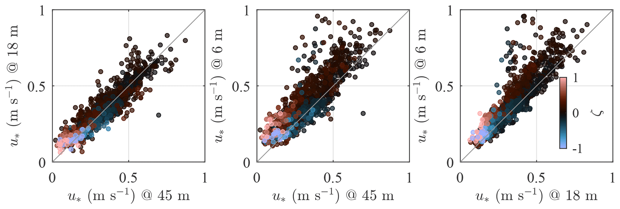
Figure 4 Friction velocity estimated by the three sonic anemometers on SMW for a wide range of stability conditions with $\left|\mathit{\zeta }\right|<\mathrm{2}$.

The applicability of MOST is assessed by studying ϕ_m as a function of ζ. The similarity relation describing the mean wind speed profile agrees well with the sonic anemometer measurements under all stability conditions except between the sensor at 6 m and 18 m a.m.s.l. at ζ>0.3. It should be noted that at 6 m a.m.s.l., the local estimate of ζ shows a much greater portion of near-neutral conditions than at 18 m a.m.s.l. The right panel of Fig. 5 does not show such a deviation, maybe because the friction velocity estimated at 45 m a.m.s.l. is slightly underestimated due to the high-frequency noise in the velocity records of the top sensor. This further justifies the use of the sonic anemometer at 18 m a.m.s.l. to estimate the non-dimensional stability parameter ζ.

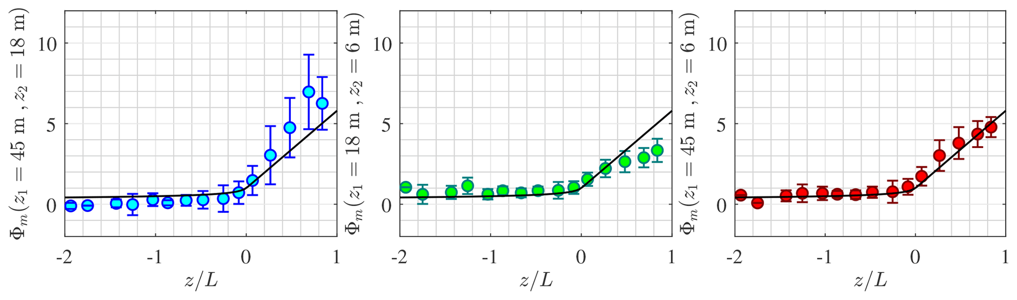
Figure 5 Variation in ϕ_m with the non-dimensional stability parameter ζ estimated from SA at 18 m a.m.s.l. The solid black line is Eq. (4), and the error bar represents the interquartile range.

The distribution of ζ as a function of the mean wind speed $\stackrel{\mathrm{‾}}{u}$ is given in Fig. 6 for the sector between 220 and 330^∘. The majority (82 %) of the stationary record samples were associated with a wind speed between 7–15 m s⁻¹ at 18 m a.m.s.l. Non-neutral conditions are defined herein as situations where $\left|\mathit{\zeta }\right|>\mathrm{0.1}$. They represent 69 % of the samples at $\stackrel{\mathrm{‾}}{u}<\mathrm{12}$ m s⁻¹ and 12 % at $\stackrel{\mathrm{‾}}{u}\ge \mathrm{12}$ m s⁻¹. The distribution of the atmospheric stability conditions is in overall agreement with Barthelmie (1999) and Sathe and Bierbooms (2007) for the Vindeby site.

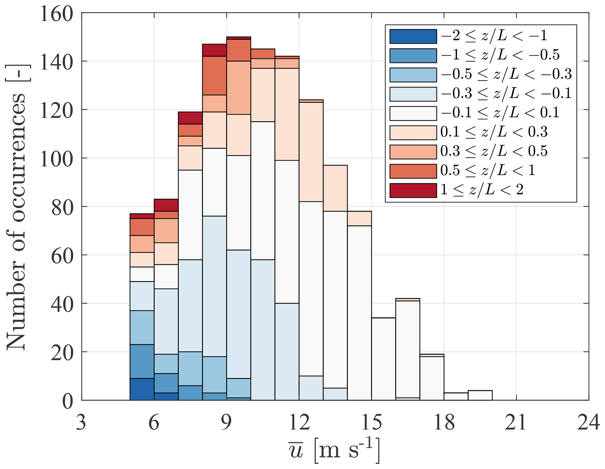
Figure 6 Stability distribution as a function of mean wind speed for the considered fetches (220–330^∘) at height z=18 m.

Strongly unstable or stable stratifications ($\left|\mathit{\zeta }\right|>\mathrm{0.5}$) made up only about 8 % of the total number of samples (Fig. 6). A low number of samples can lead to large uncertainties when comparing the flow characteristics between SMW and FINO1 for specific stability bins. Therefore, only stability conditions satisfying $\left|\mathit{\zeta }\right|\le \mathrm{0.5}$ are discussed herein unless indicated otherwise.

5.2 Wind–wave interactions

The fairly close proximity of the sensor at 6 m to the sea surface is used to study the potential influence of the wave boundary layer (WBL) (Sjöblom and Smedman, 2003a). This layer is also called the wave sublayer by Emeis and Türk (2009), who suggest that its depth is approximately 5H_s, although there is no consensus on this value. The objective of this subsection is to identify whether the wave-induced turbulence can be detected in the velocity records at 6 m a.m.s.l.

The wave elevation data collected by the AWR near SMW are explored herein in terms of wind–wave interactions. A total of 925 high-quality samples collocated in time with the wind velocity data were identified. Each wave elevation record was 30 min long and corresponded to a wind direction between 220 and 330^∘. There exist methods to filter out the wave-induced velocity component from the turbulent velocity component (e.g. Hristov et al., 1998), but these methods are not addressed herein for brevity.

The interactions between wind turbulence and the sea surface were explored in terms of the co-coherence and the quad-coherence (the imaginary part of the root coherence) between the vertical velocity component w and the velocity of the wave surface $\dot{\mathit{\eta }}=\mathrm{d}\mathit{\eta }/\mathrm{d}t$. Similar approaches were adopted earlier by, for example, Grare et al. (2013) or Kondo et al. (1972) but using the coherence and without taking advantage of the ensemble average to reduce the systematic and random error, which are typically associated with the root-coherence function. In the present case, neither the co-coherence nor the quad-coherence between $\dot{\mathit{\eta }}$ and w differs significantly from zero for H_s<0.7 m. For the sensor at 6 m a.m.s.l., a non-zero root coherence was discernible from the background noise at 0.7 m < H_s < 0.9 m. The co-coherence and quad-coherence estimates were significantly different from zero for H_s>0.9 m, as illustrated in Fig. 7, where the ensemble averaging of the 60 samples was applied to reduce the random error. The inset in Fig. 7 shows that the selected records are characterised by a single spectral peak f_p located at frequencies between 0.20 and 0.25 Hz, which is the frequency range where the quad-coherence is substantially different from zero. The observed co-coherence and the quad-coherence at this frequency range show the 90^∘ out-of-phase fluctuations between $\dot{\mathit{\eta }}$ and w, where the latter is lagging. The co-coherence and quad-coherence estimates between $\dot{\mathit{\eta }}$ and the horizontal wind component u were also investigated but were nearly zero for the three sonic anemometers on SMW.

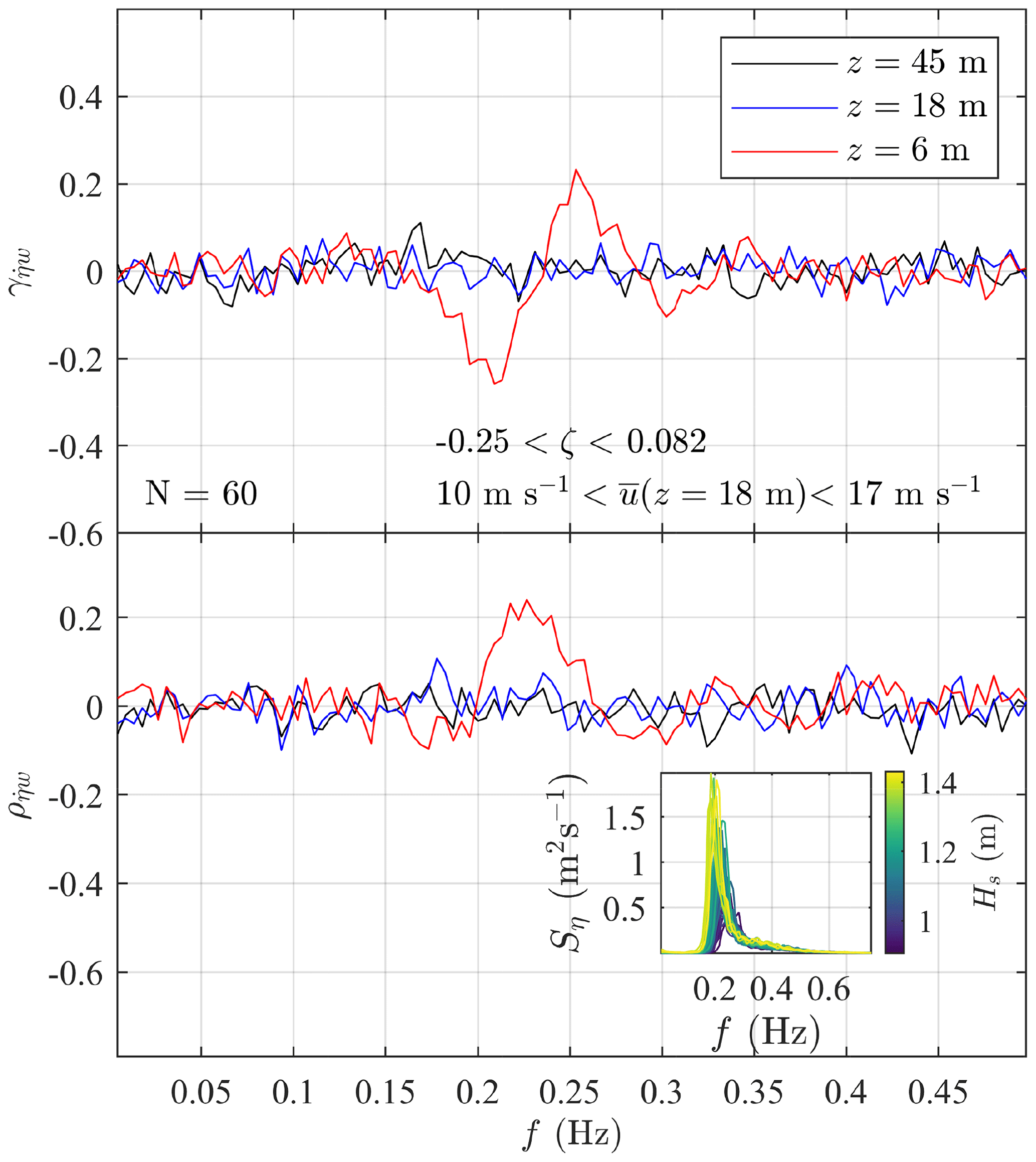
Figure 7 Co-coherence ${\mathit{\gamma }}_{\dot{\mathit{\eta }}\mathrm{w}}$ and quad-coherence ${\mathit{\rho }}_{\dot{\mathit{\eta }}\mathrm{w}}$ between the velocity of the wave surface $\dot{\mathit{\eta }}$ and the vertical wind velocity w from the three sonic anemometers on SMW. The inset shows the individual wave elevation spectra S_η associated with H_s>0.9 m (60 samples) used to estimate ${\mathit{\gamma }}_{\dot{\mathit{\eta }}\mathrm{w}}$ and ${\mathit{\rho }}_{\dot{\mathit{\eta }}\mathrm{w}}$.

The limited number of data showing a clear correlation between the velocity of the sea surface and the vertical wind component implies that the wave-induced turbulence has a limited impact on the anemometer records at 6 m. The influence of the sea surface elevation on the vertical turbulence was not clearly visible in the one-point vertical velocity spectra S_w, except for at H_s>1.2 m, where a weak spectral peak near 0.2 Hz was distinguishable. The wave-induced fluctuating wind component is generally much weaker compared to the wind turbulence as highlighted by, for example, Weiler and Burling (1967), Kondo et al. (1972) and Naito (1983). An exception may be the case of weak wind and swell conditions, which are more likely to result in the observation of a sharp spectral peak near f_p in the S_w spectrum (Kondo et al., 1972). Nonetheless, as previously mentioned, such conditions are rare near SMW, most likely because SMW was located in a relatively sheltered closed-water environment rather than in the open ocean.

5.3 Turbulence spectra

When performing numerical simulations to compute the wind-induced response of wind turbines, an essential input to model the wind inflow conditions is the PSD of the velocity fluctuations. Figures 8–10 depict the PSD estimates for the along-wind, cross-wind, and vertical wind components, respectively, as a function of the reduced frequency f_r for five stability classes. Surface-layer scaling is adopted; i.e. the PSDs are normalised with u_* (Eq. 2) and ${\mathit{\varphi }}_{\mathit{ϵ}}^{\mathrm{2}/\mathrm{3}}$ (Eq. 8). The number of available samples for each stability class is denoted as N and displayed in each panel.

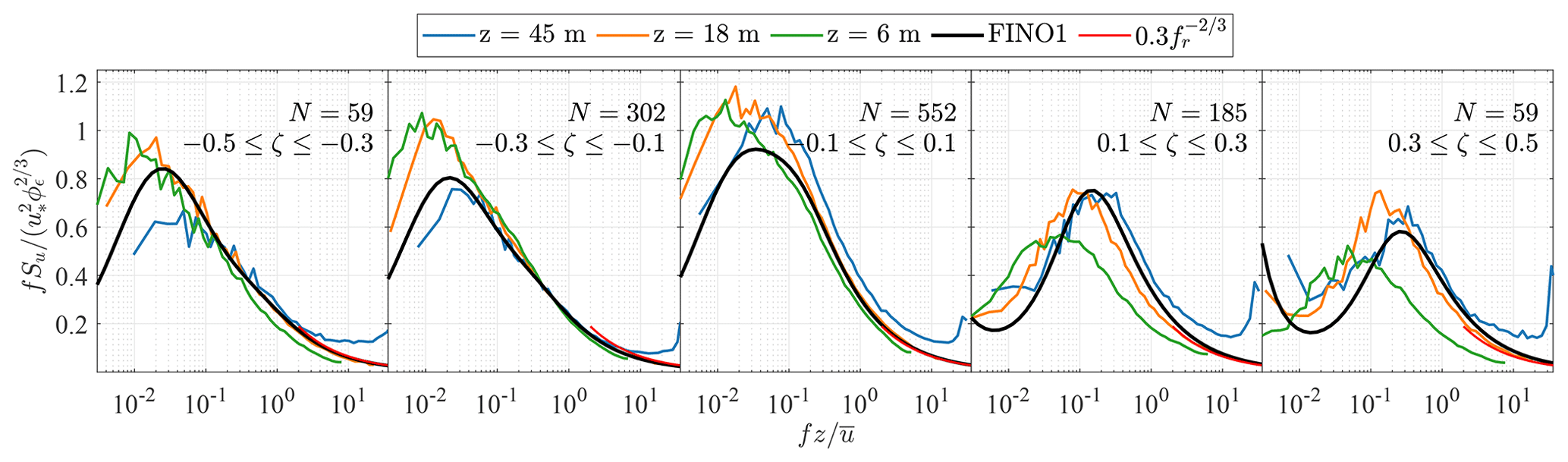
Figure 8 Normalised spectra of the along-wind component at 45, 18, and 6 m a.m.s.l. for various stability conditions. The red curve is derived from Eq. (5), and N denotes the number of samples considered for ensemble averaging.

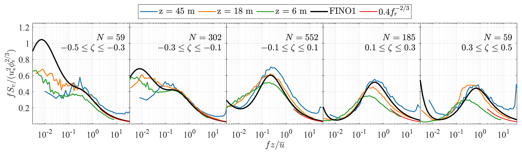
Figure 9 Normalised spectra of the cross-wind component at 45, 18, and 6 m a.m.s.l. for various stability conditions. The red curve is derived from Eq. (6), and N denotes the number of samples considered for ensemble averaging.

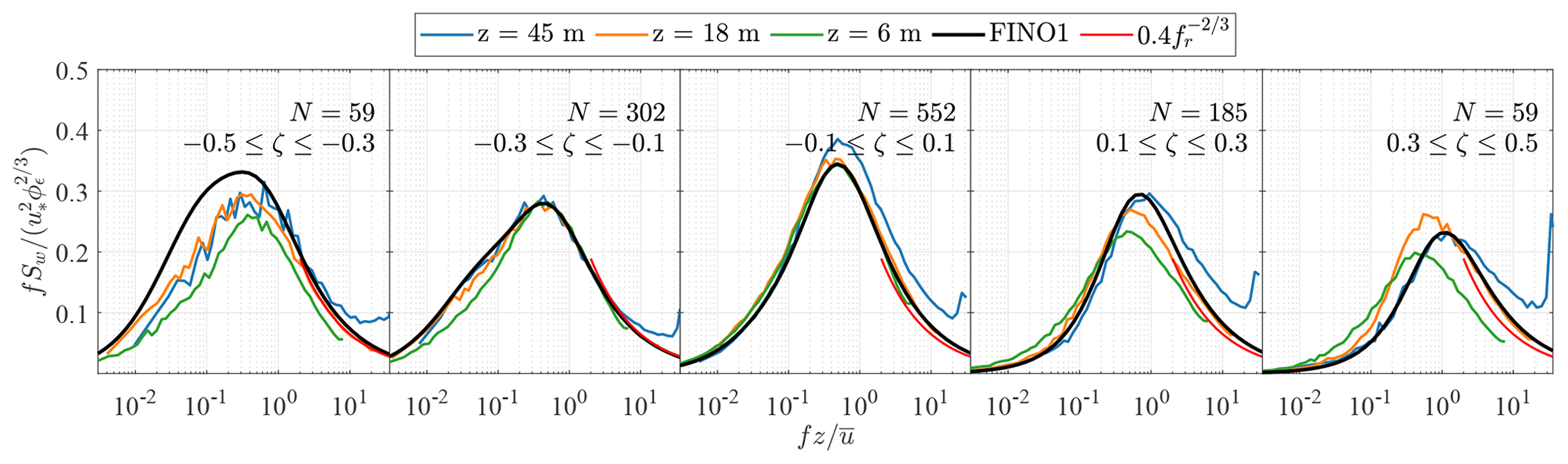
Figure 10 Normalised spectra of the vertical wind component at 45, 18, and 6 m a.m.s.l. for various stability conditions. The red curve is derived from Eq. (6), and N denotes the number of samples considered for ensemble averaging.

Figures 8 to 10 compare the estimated spectra at z=45 m, z=18 m, and z=6 m a.m.s.l. with the empirical model established on FINO1 (solid black line) at z=41 m a.m.s.l. (Cheynet et al., 2018). The red curves represent the high-frequency asymptotic behaviour of surface-layer spectra for each stability class. It should be noted that the latter curves do not indicate when the inertial subrange starts since the frequencies they cover were arbitrarily chosen.

In Fig. 8, the maximum values of the normalised spectra for near-neutral conditions ($-\mathrm{0.1}\le \mathit{\zeta }\le \mathrm{0.1}$) are close to unity, as described by Kaimal et al. (1972). The velocity spectra estimated at 45 m a.m.s.l. sometimes show deviations from the surface-layer scaling under near-neutral and stable conditions, likely due to the observed aforementioned uncorrelated high-frequency noise, which leads to an underestimation of the friction velocity. Under light and moderate unstable conditions, i.e. $-\mathrm{0.3}\le \mathit{\zeta }\le -\mathrm{0.1}$, the velocity spectra at 6 m and 18 m a.m.s.l. are similar, which supports the idea that the wave sublayer is shallower than 6 m. As mentioned in Sect. 5.1, the non-dimensional stability parameter ζ estimated at 6 m reflected the predominance of near-neutral conditions. This results in discrepancies between the spectral estimates at 6 and 18 m in Figs. 8 to 10 which increase with $\left|\mathit{\zeta }\right|$.

Following surface-layer scaling, the normalised spectra at different heights should collapse onto one single curve at high frequencies, which was observed at heights between 40 and 80 m a.m.s.l., at FINO1 for $\left|\mathit{\zeta }\right|<\mathrm{1}$. However, this is not always the case in Figs. 8–10. Deviations from surface-layer scaling may be partly attributed to transducer-induced flow distortion. Regarding the velocity data at 45 m a.m.s.l., the measurement noises lift the high-frequency range of the velocity spectra above the spectral slope predicted by Eq. (5) or Eq. (6). At 18 m a.m.s.l., Eqs. (5) and (6) predict remarkably well the velocity spectra at f_r>3, indicating that surface-layer scaling is applicable at this height.

The presence of the spectral gap (Van der Hoven, 1957), separating the microscale fluctuations from the sub-mesoscale and mesoscale ones, is noticeable at ζ>0.3, in line with previous observations (Smedman-Högström and Högström, 1975; Cheynet et al., 2018). Under stable conditions, the spectral gap seems to move toward lower frequencies as the height above the surface decreases. This contrasts with the observations from an onshore mast on Østerild (Denmark) by Larsén et al. (2018), which indicated that the location of the spectral gap on the frequency axis was relatively constant with height.

As mentioned by Vickers and Mahrt (2003), the spectral gap timescale can be only a few minutes long under stable conditions. For ζ>0.3, the averaging period selected in the present study may be too large to provide reliable integral turbulence characteristics. However, filtering out the mesoscale motion may not be desirable for structural design purposes since operating wind turbines experience both turbulence and mesoscale fluctuations (Veers et al., 2019). In this regard, the use of spectral flow characteristics to parametrise the wind loading on OWTs is preferable.

Under near-neutral conditions, the sensors at 6 and 18 m a.m.s.l. are likely located in the so-called eddy surface layer (Högström et al., 2002; Drobinski et al., 2004), where the sea surface blocks the flow and distorts eddies. This leads to a flat spectral peak. As a result, the integral length scale would be estimated with large uncertainties. Such a spectral behaviour has also been observed above the eddy surface layer (Drobinski et al., 2004; Mikkelsen et al., 2017), but its consequences for wind turbine loads are unclear.

Overall, the velocity spectra estimated at 18 and 45 m a.m.s.l. at Vindeby match well with the empirical spectra estimated at 41 m a.m.s.l. on FINO1 for $-\mathrm{0.5}\le \mathit{\zeta }<\mathrm{0.5}$. This comparison is encouraging for further explorations of the surface-layer turbulence characteristics at coastal and offshore sites. Nonetheless, detailed wind measurements at heights of z≥100 m are needed to obtain a complete overview of the turbulence characteristics in the MABL that is relevant for OWT designs.

Figure 11 Co-coherences of the along-wind (top panels), lateral (middle panels), and vertical velocity components (lower panels) for $\left|\mathit{\zeta }\right|\le \mathrm{0.1}$ at three different vertical separation distances. The dots represent the measurement, and the lines mark the predictions using the IEC exponential coherence model (dashed line) and the modified Bowen model (solid line) with the fitted coefficients from FINO1 (Cheynet, 2019).

5.4 Co-coherence of turbulence

The vertical co-coherence of the along-wind, cross-wind, and vertical wind components are denoted by γ_u, γ_v, and γ_w, respectively. Under near-neutral conditions ($\left|\mathit{\zeta }\right|\le \mathrm{0.1}$), these are expressed as a function of kd_z in Fig. 11 where $k=\mathrm{2}\mathit{\pi }f/\stackrel{\mathrm{‾}}{u}$ is the wave number, assuming that turbulence is frozen (Taylor, 1938). The co-coherence estimates are presented for three separation distances d_z because three measurement heights (z₁=45 m, z₂=18 m, and z₃=6 m) were used. The co-coherences estimated on SMW are compared to the IEC coherence model (Eq. 16) and the modified Bowen model (Eq. 13). For the latter model, the parameters estimated on FINO1 (Cheynet, 2019) are directly used. The decay coefficients used for Eq. (13) were, therefore, $[c_{\mathrm{1}}^{\mathrm{u}},c_{\mathrm{2}}^{\mathrm{u}},c_{\mathrm{3}}^{\mathrm{u}}]=[\mathrm{6.0},\mathrm{17.8},\mathrm{0.02}]$ and $[c_{\mathrm{1}}^{\mathrm{w}},c_{\mathrm{2}}^{\mathrm{w}},c_{\mathrm{3}}^{\mathrm{w}}]=[\mathrm{2.7},\mathrm{4.0},\mathrm{0.16}]$ as well as $[c_{\mathrm{1}}^{\mathrm{v}},c_{\mathrm{2}}^{\mathrm{v}},c_{\mathrm{3}}^{\mathrm{v}}]=[\mathrm{0},\mathrm{23.0},\mathrm{0.09}]$.

Figure 11 shows that the coefficients of the modified Bowen model estimated on FINO1 apply very well to γ_u estimated on SMW. Larger deviations are observed for the cross-wind components, for which γ_v displays large negative values, especially for separations between 6 and 45 m a.m.s.l. At FINO1, the negative part of γ_v was relatively small, which justified the use of Eq. (13) with no negative co-coherence values. Following Bowen et al. (1983), ESDU 85020 (2002), or Chougule et al. (2012), the negative part is a consequence of the phase difference and is non-negligible for the cross-wind component, which is also observed in the present case. Since this phase difference increases with the mean wind shear, it is more visible at SMW than at FINO1, where the measurements are at greater heights than at SMW. The co-coherence of the vertical component estimated on SMW deviates from the one fitted to observations at the FINO platform. The source of such deviations remains unclear.

The IEC exponential coherence model over-predicts γ_u when the measurement height decreases and when the separation distance increases because this model follows fairly well Davenport's similarity, except at kd_z<0.1. In Cheynet (2019), the Davenport model was suspected to lead to an overestimation of the turbulent wind loading on OWTs. The present results indicate that a similar overestimation may be obtained if the IEC exponential coherence model is used. Further studies are, however, needed to better quantify this possible overestimation in terms of dynamic wind loading on the wind turbine's rotor and tower, as well as on the floater's motions in the case of a floating wind turbine. Finally, additional data collection is needed to study the co-coherence at lateral separations, which is required for wind turbine design since it was not available at FINO1 or SMW.

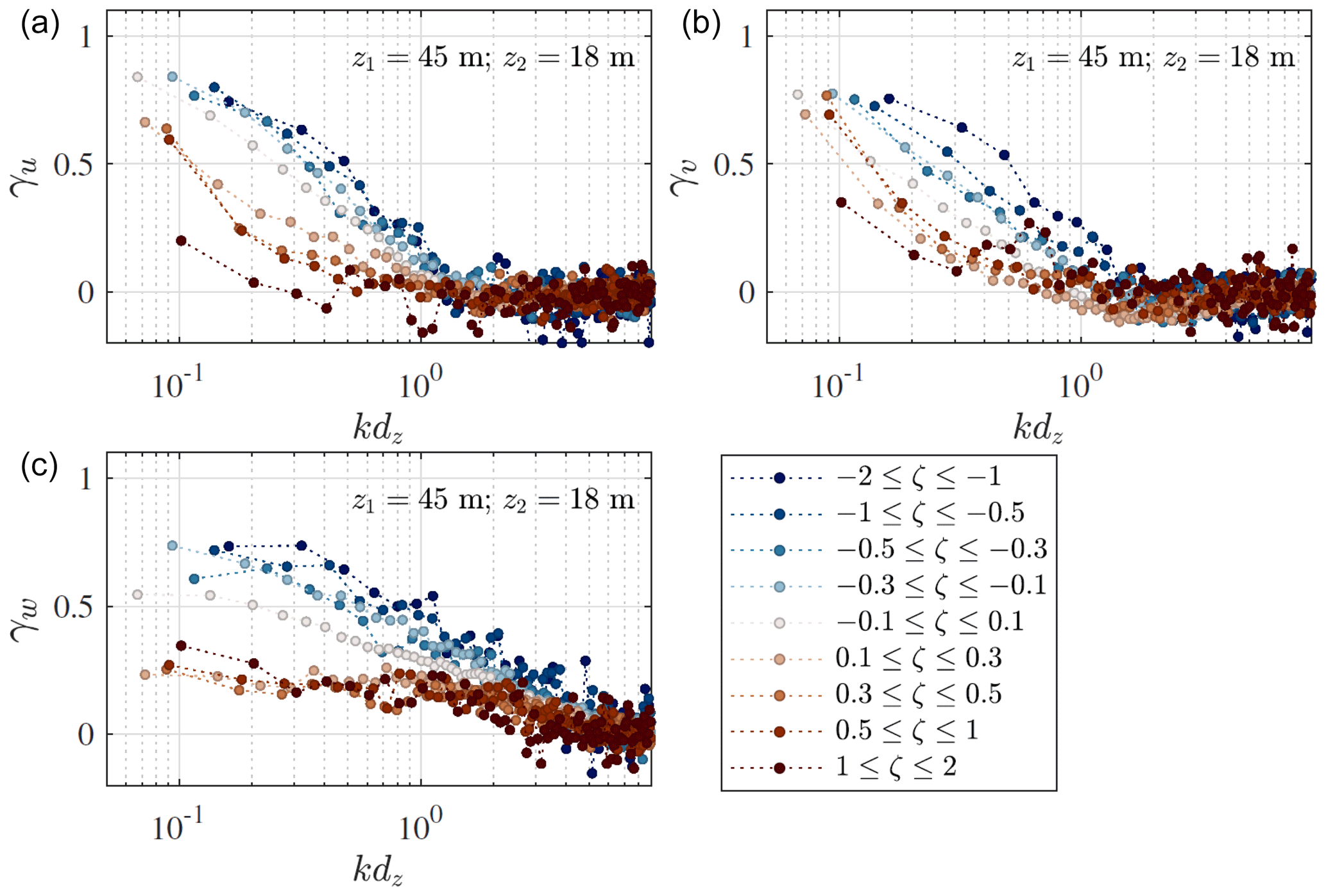
Figure 12 Co-coherence of the along-wind (a), cross-wind (b), and vertical (c) velocity components for nine stability classes, given by $\mathit{\zeta }=z/L$. The separation distance is 27 m between the sensors at 18 m and 45 m a.m.s.l.

To demonstrate the effect of the thermal stratification on the observed co-coherence at SMW, Fig. 12 shows the estimated co-coherence for $-\mathrm{2}\le \mathit{\zeta }\le \mathrm{2}$ for the three turbulence components. As observed by, for example, Soucy et al. (1982) or Cheynet et al. (2018) and modelled by Chougule et al. (2018), the vertical co-coherence is generally highest for convective conditions and smallest for stable conditions. Such results reinforce the idea that modelling the turbulent loading on offshore wind turbines using a coherence model established for neutral conditions may only be appropriate for the ultimate limit state design but not for the fatigue life design.

5.5 Relevancy of the database for load calculation of OWTs

This study provides a thorough overview of the MABL spectral turbulence characteristics with respect to the variation in the atmospheric stability at SMW. However, its direct applicability for the designs of OWTs should be assessed carefully due to the assumptions made in the data analysis.

The presented results do not include the non-stationary conditions encountered in the field, which were removed before the analysis. About 20 % of the data were disregarded as non-stationary to establish reliable spectra and co-coherence estimates. In the present case, non-stationary fluctuations were mainly associated with frequencies close to or below 0.05 Hz. For typical spar-type and semisubmersible OWT floaters, these frequencies encompass the quasi-static motions and a few of the lowest eigenfrequencies of the floaters (Jonkman and Musial, 2010; Robertson et al., 2014). Additionally, the non-stationary turbulence fluctuations could result in non-Gaussian loadings, which could further lead to underestimation of fatigue loading (Benasciutti and Tovo, 2006, 2007).

Furthermore, the present dataset was recorded at heights lower than the hub height of the recent and the future OWTs, which is around 130 m (e.g. GE Renewable Energy, 2021). At such heights, MOST may no longer be applicable (Peña and Gryning, 2008; Cheynet et al., 2021). Above the surface layer, the velocity spectra may become independent of the height above the surface, which is coarsely accounted for in IEC 61400-1 (2005).

6 Conclusions

This study explores the turbulence spectral characteristics from wind records of a year duration on an offshore mast called Sea Mast West (SMW) near the first offshore wind farm Vindeby. We aim to identify similarities between the turbulence characteristics estimated on the FINO1 platform in the North Sea and those at Vindeby. Such an investigation is crucial to establish appropriate turbulence models relevant for the design of offshore wind turbines (OWTs). The dataset analysed was acquired by 3D sonic anemometers at 6, 18, and 45 m a.m.s.l., which complements the dataset collected between 40 m and 80 m a.m.s.l. on FINO1 (Cheynet et al., 2018).

The correlation between the sea surface elevation and the vertical turbulent fluctuations at 6 m a.m.s.l. is quantified in terms of co-coherence between the vertical turbulent component and the velocity of the sea surface elevation. However, it is clearly visible for significant wave heights H_s exceeding 0.9 m only. Therefore, it is concluded that the sonic anemometers are located above the wave boundary layer most of the time.

The measurements at 18 m a.m.s.l. follow fairly well surface-layer scaling, as expected. Because the sensors at 6 and 18 m are located in the lower part of the surface layer, a wide spectral peak for near-neutral stratification is observed, which reflects the distortion of the eddies as they scrape along the surface. For $\mathit{\zeta }=|z/L|\le \mathrm{0.3}$, the power spectral density of the along-wind velocity component at 18 and 45 m is consistent with the empirically defined spectral models estimated at 41 m on FINO1 (Cheynet et al., 2018). In the present case, most of the wind records are associated with $\left|\mathit{\zeta }\right|<\mathrm{0.3}$. Nonetheless, for $\left|\mathit{\zeta }\right|>\mathrm{0.3}$, deviations from the empirical spectral model fitted to the data recorded on the FINO1 platform may be attributed to transducer-induced flow distortion and/or limited applicability of the surface-layer scaling.

The co-coherence estimates of the along-wind component for neutral atmospheres are well described by the same three-parameter exponential decay function as used at FINO1 (Cheynet, 2019). However, this is not the case for the lateral wind components due to the closer distance to the sea surface, which amplifies the phase differences between measurements at two different heights. For the vertical component, the co-coherence decreases faster than the predicted values at FINO1 (Cheynet et al., 2018). Under stable stratification, the co-coherence estimates of the three turbulent components (γ_u, γ_v, and γ_w) are significantly lower than for near-neutral conditions, in particular for kd_z<1. On the other hand, γ_u, γ_v, and γ_w are slightly higher for convective conditions compared to near-neutral conditions at kd_z<1. Since the co-coherence is one of the governing parameters for wind loading on structures, its dependency on the atmospheric stability, which is rarely documented in the marine atmospheric boundary layer, may become essential to establishing design criteria for OWT fatigue life. The variability in Hywind Scotland wind turbines’ floater motion with atmospheric stability (Jacobsen and Godvik, 2021) may be one example that demonstrates the importance of stability-corrected co-coherence in OWT responses.

Although the Vindeby dataset is located below recent wind turbines' sizes, this does not mean that the dataset may not be useful for wind turbine design purposes. In fact, the widely known Kansas spectra were based on the observations at heights not exceeding 30 m (Kaimal et al., 1972) and have been adopted in IEC 61400-1 (2005). From the Vindeby dataset, we found some similarities with the Kansas spectra for near-neutral conditions. For non-neutral conditions, the turbulence spectra at height 45 m a.m.s.l. have a consistent behaviour with the predicted spectra at FINO1 at 41.5 m a.m.s.l. The comparison between the turbulence characteristics at Vindeby and FINO1 is therefore valuable to further develop comprehensive spectral turbulence models that are suitable for modern OWT designs. Nevertheless, future atmospheric measurements at heights up to 250 m a.m.s.l. are necessary to obtain the knowledge of turbulence characteristics where the surface-layer scaling may no longer be applicable.

Appendix A: Sonic anemometer tilt correction

The friction velocity estimates using the double-rotation technique, sectoral planar fit, and the method by Klipp (2018) are compared in Fig. A1. In general, the friction velocity estimates from all methods are in good agreement. The average correlation coefficient for all heights is 0.985 for $\left|\mathit{\zeta }\right|\le \mathrm{2}$. The PF algorithm leads to a slightly larger scatter between u_*R and u_*, where the average correlation coefficient from all heights is 0.976 for $\left|\mathit{\zeta }\right|\le \mathrm{2}$ (Table A1). The double-rotation algorithm seems to give a smaller deviation between u_*R and u_* than the PF algorithm in the present study, which justified the adoption of the double rotation as a tilt correction method herein.

Klipp (2018) noted that u_*R is appropriate to estimate the friction velocity if the thermal stratification of the atmosphere is neutral only. Yet, Fig. A1 suggests that Klipp's method performs well for non-neutral conditions too, as highlighted by the correlation coefficients in Table A1, which vary between 0.963 and 0.989. Additional studies using measurements from other coastal or offshore sites are needed to assess if such observations are recurring.

The angle between the stress vector and the wind vector is given as $\mathit{\alpha }=\arctan \left(\stackrel{\mathrm{‾}}{v^{\prime }{w}^{\prime }}/\stackrel{\mathrm{‾}}{u^{\prime }{w}^{\prime }}\right)$ (Grachev et al., 2003). It is found that α increases from 8^∘ at 6 m a.m.s.l. to 13^∘ at 45 m a.m.s.l. when $\stackrel{\mathrm{‾}}{v^{\prime }{w}^{\prime }}<\mathrm{0}$. When $\stackrel{\mathrm{‾}}{v^{\prime }{w}^{\prime }}>\mathrm{0}$, α is almost constant with the height with an average value of −7^∘. The relatively low value of α, therefore, suggests that the direction of the wind–wave-induced stress is fairly well aligned with the mean wind direction near SMW.

Table A1 Correlation coefficients between u_*R and u_* using the planar fit (PF) or double rotation (DR).

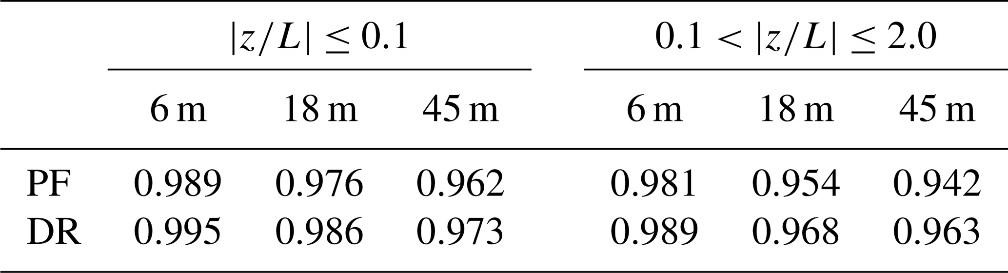
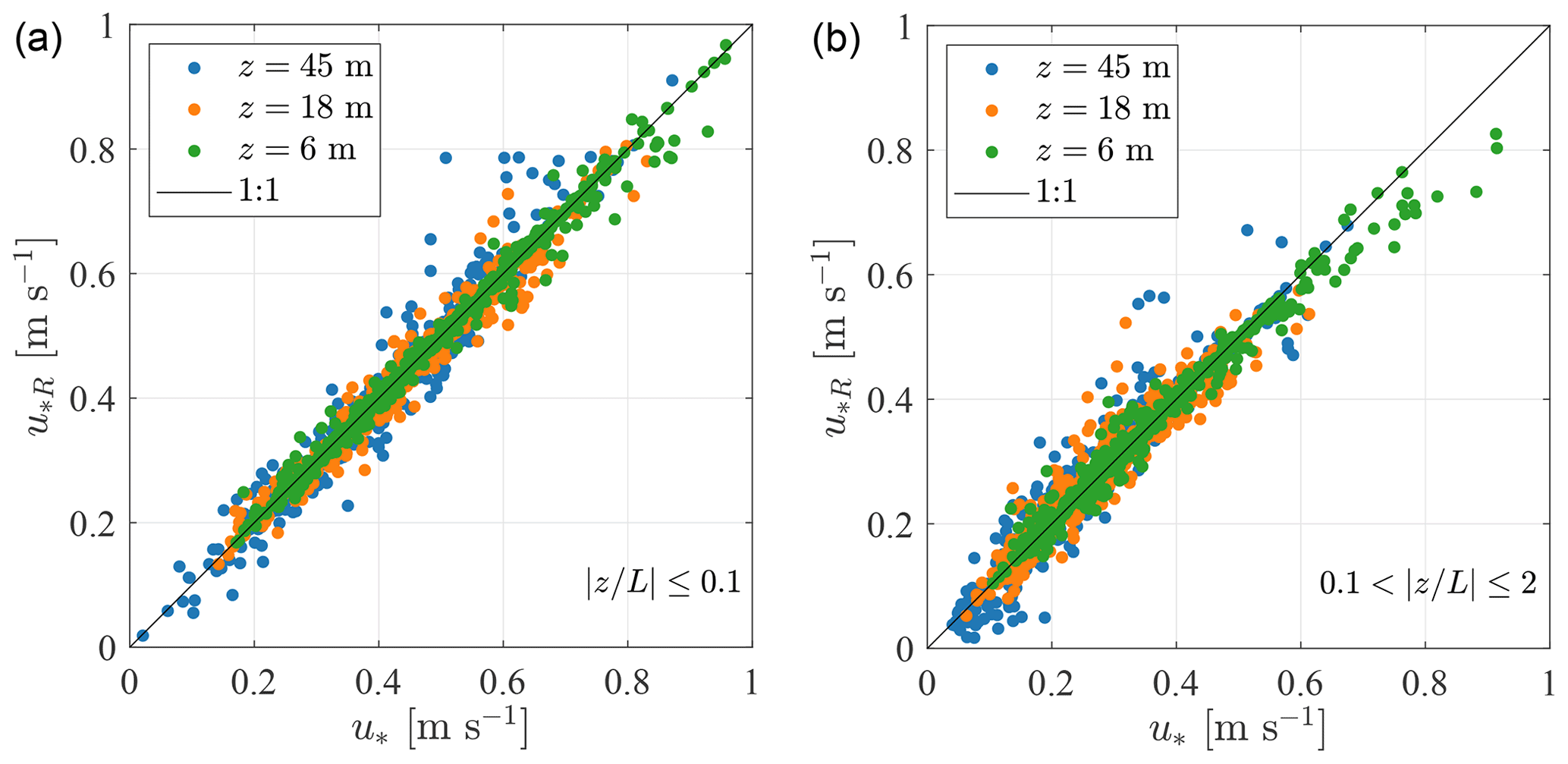
Figure A1 Friction velocity computed using the eddy covariance method with the double-rotation method compared with the Klipp method. Panel (a) considers only $|z/L|\le \mathrm{0.1}$, and panel (b) considers $\mathrm{0.1}<|z/L|\le \mathrm{2}$.

Appendix B: Transducer-shadow effect

The sonic anemometers mounted at 6, 18, and 45 m a.m.s.l. were omnidirectional solent anemometers, which can be prone to flow distortion by the transducer. Between May and September 1994, a Gill solent anemometer with an asymmetric head was installed at 10 m a.m.s.l. on the southern boom of SMW (i.e. on the same side as the other three anemometers). The asymmetric head reduces the flow distortion by the transducer, at least for a specific wind sector. Although the flow distortion by the asymmetric solent was actually unknown, this sensor was used to assess the error in the friction velocity calculated with the omnidirectional solent anemometers. Only wind directions from 220 to 330^∘ were selected as they corresponded to the sector investigated in the present study.

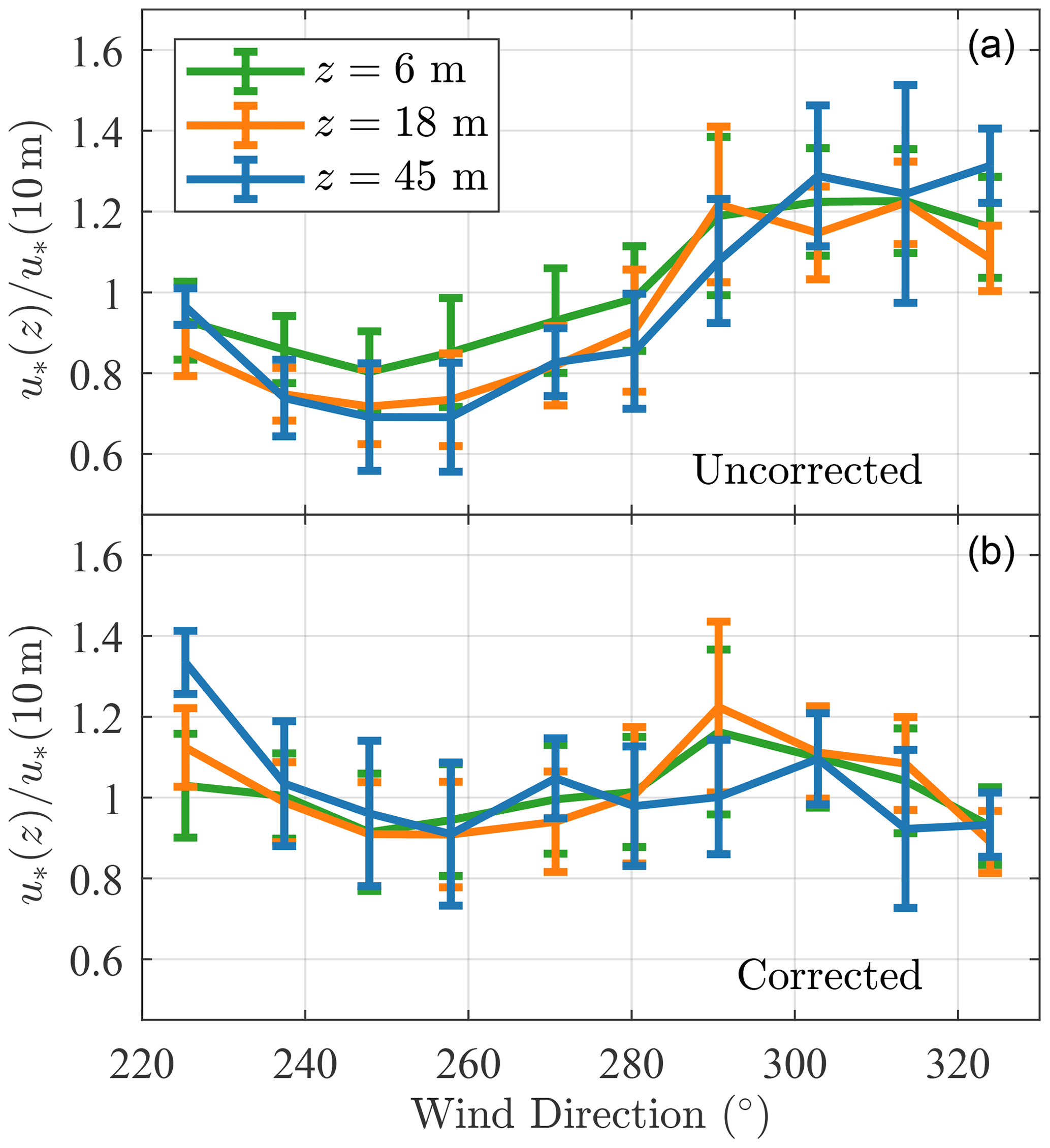
Figure B1 Ratio of the friction velocity by the omnidirectional solent anemometers to the one estimated at 10 m (asymmetric solent anemometer) before (a) and after (b) correction using a multivariate regression analysis. Velocity data recorded between May and September 1994 for the sector 220–330^∘ were used (480 samples of 30 min duration), and $|z/L|<\mathrm{2}$ at 10 m a.m.s.l.

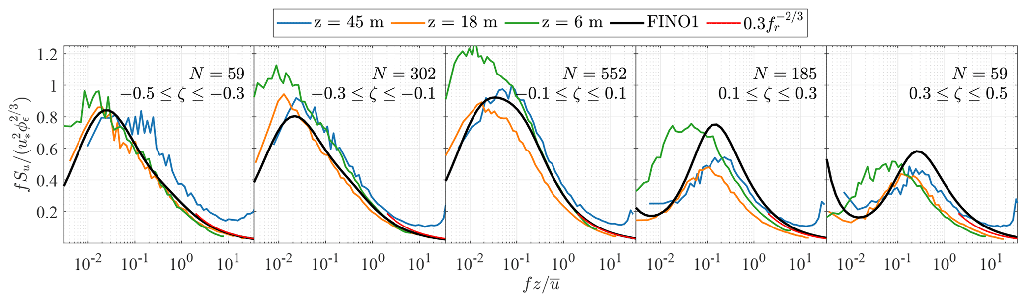
Figure B2 Normalised spectra of the along-wind component on SMW with the corrected friction velocity and five stability bins. The red curve is derived from Eq. (5), and N denotes the number of samples considered for ensemble averaging.

Flow distortion is assumed to be a function of the angle of attack α(z) and wind direction θ(z) only. Therefore, using a multivariate regression analysis, it is possible to quantify the variability in u_*(z) with its value at 10 m, denoted (u_*)₁₀, as a function of α(z) and θ(z). For the relatively narrow sector selected, it was found that cubic functions of α(z) and θ(z) were sufficient to describe this variability. This leads to the following relationship between the friction velocity at 10 m and the one u_* at height z:

$$\begin{array}{}\text{(B1)}& u_{*}\left(z\right)={\left(u_{*}\right)}_{\mathrm{10}}\cdot {\mathbf{AX}}^{\top },\end{array}$$

$$\begin{array}{}\text{(B2)}& {\displaystyle }& {\displaystyle }\mathbf{A}=\left[\begin{array}{cccccc}{a}_{\mathrm{1}}& a_{\mathrm{2}}& a_{\mathrm{3}}& a_{\mathrm{4}}& a_{\mathrm{5}}& a_{\mathrm{6}}\end{array}\right],\text{(B3)}& {\displaystyle }& {\displaystyle }\mathbf{X}=\left[\begin{array}{cccccc}\mathit{\theta }\left(z\right)& \mathit{\theta }(z{)}^{\mathrm{2}}& \mathit{\theta }(z{)}^{\mathrm{3}}& \mathit{\alpha }\left(z\right)& \mathit{\alpha }(z{)}^{\mathrm{2}}& \mathit{\alpha }(z{)}^{\mathrm{3}}\end{array}\right],\end{array}$$

where A is the matrix of coefficients to be determined with the regression analysis. In Eqs. (B1)–(B3), the friction velocity is not forced to be constant with the height and we do not assume that the flow distortion is similar for the three omnidirectional anemometers.

In the top panel of Fig. B1, the maximum variations in the friction velocity between the sonic anemometer at 10 and 18 m are ±20 %, when all the samples in the sector 10 m are 4 %, 12 %, and 11 %, respectively. After the multivariate regression, the sector-averaged error is nearly zero, although it is clearly not zero for a given wind direction. On average, the friction velocity estimates at 6 and 10 m are, therefore, almost identical, given that the random error in the friction velocity is above 10 % for a sample duration of 30 min (Kaimal and Finnigan, 1994). As shown in Fig. B1, the use of sector-averaged flow characteristics may mitigate the influence of transducer-induced flow distortion of the spectral flow characteristics estimated at 6, 18, and 45 m.

A comparison of the power spectral densities of the u component was conducted with and without the corrected friction velocity. Only data between May and September 1994 were selected, and the Obukhov length was computed at 10 m a.m.s.l. Five stability bins were identified in this dataset. However, limited improvement was observed after the application of the correction algorithm. A further comparison was also conducted for the entire dataset, i.e. between May 1994 and July 1995, as shown in Fig. B2. This resulted in similar conclusions, where the uncorrected (Fig. 8) and the corrected PSDs of the u component are not too far off each other. Therefore, it was decided not to use any correction for the friction velocity to avoid over-processing the data.