Experimental analysis of the dynamic inflow effect due to coherent gusts

The dynamic inflow effect describes the unsteady aerodynamic response to fast changes in rotor loading due to the inertia of the wake. Fast changes in turbine loading due to pitch actuation or rotor speed transients lead to load overshoots. The phenomenon is suspected to be also relevant for gust situations; however, this was never shown, and thus the actual load response is also unknown. The paper's objectives are to prove and explain the dynamic inflow effect due to gusts, and compare and subsequently improve a typical dynamic inflow engineering model to the measurements. An active grid is used to impress a 1.8 m diameter model turbine with rotor uniform gusts of the wind tunnel flow. The influence attributed to the dynamic inflow effect is isolated from the comparison of two experimental cases. Firstly, dynamic measurements of loads and radially resolved axial velocities in the rotor plane during a gust situation are performed. Secondly, corresponding quantities are linearly interpolated for the gust wind speed from lookup tables with steady operational points. Furthermore, simulations with a typical blade element momentum code and a higher-fidelity free-vortex wake model are performed. Both the experiment and higher-fidelity model show a dynamic inflow effect due to gusts in the loads and axial velocities. An amplification of induced velocities causes reduced load amplitudes. Consequently, fatigue loading would be lower. This amplification originates from wake inertia. It is influenced by the coherent gust pushed through the rotor like a turbulent box. The wake is superimposed on that coherent gust box, and thus the inertia of the wake and consequently also the flow in the rotor plane is affected. Contemporary dynamic inflow models inherently assume a constant wind velocity. They filter the induced velocity and thus cannot predict the observed amplification of the induced velocity. The commonly used Øye engineering model predicts increased gust load amplitudes and thus higher fatigue loads. With an extra filter term on the quasi-steady wind velocity, the qualitative behaviour observed experimentally and numerically can be caught. In conclusion, these new experimental findings on dynamic inflow due to gusts and improvements to the Øye model enable improvements in wind turbine design by less conservative fatigue loads.

1 Introduction

The dynamic inflow phenomenon is an unsteady aerodynamic effect relevant for helicopters (Peters, 2009) and wind turbines (Snel and Schepers, 1994). It is considered for a fast load variation through a blade pitch step or fast change in rotor speed. Due to the inertia of the wake, the induced velocity cannot change instantaneously but only gradually to a fast load event in the rotor plane. This dynamic transition in the wake leads to load and power overshoots between the two steady states. For wind turbines, Snel and Schepers (1994) also suspect variations in inflow velocity, especially due to coherent wind gusts, to lead to relevant dynamic inflow effects.

Aeroservoelastic simulations are used to obtain relevant turbine loads in the design and certification process of wind turbines. The aerodynamic part of these simulations is based on the blade element momentum (BEM) theory that gives the aerodynamic forces acting on the rotor blade segments. BEM, however, is inherently based on steady-flow assumptions, and engineering models are needed to catch dynamic phenomena, like the dynamic inflow effect. Widely used examples are the ECN model (Snel and Schepers, 1994) in Phatas and the ECN (now TNO) Aero-Module, the recent DTU model (Madsen et al., 2020) in HAWC2, and the Øye model (Øye, 1986, 1990; Snel and Schepers, 1994) in GH Bladed and OpenFAST. They all have the main working mechanism that they filter the induced velocity based on time constants. One time constant is used for the ECN model and two time constants for the DTU and Øye model.

In addition to the need of engineering models for dynamic inflow effects, blade element momentum (BEM) theory is based on the assumption of axial and uniform inflow. Free-vortex wake methods (FVWMs) on the other hand model dynamic inflow effects and also non-uniform inflow intrinsically. Boorsma et al. (2020) looked at the influence of turbulent wind fields with shear on the loading of wind turbines. They found relevant lower fatigue loading for the out-of-plane blade root bending moments and tower bottom fore–aft bending moment for the higher-fidelity FVWM-type simulations, compared to BEM-type simulations. The implementation of how non-uniform inflow influences the induced velocities over one rotation in BEM was identified as one relevant contribution to this behaviour; however, they also suspected the dynamic inflow effect to be responsible for some of the differences between BEM and FVWM in turbulent inflow.

Within two historic EU projects on dynamic inflow (Snel and Schepers, 1994; Schepers and Snel, 1995) a 1.2 m diameter model wind turbine was exposed to a step change in wind velocity generated by a manually operated gust generator in a wind tunnel. This experiment did not observe a dynamic inflow effect due to gusts. Snel and Schepers (1994) related this to the slow step change in wind velocity, compared to the typical dynamic inflow time constant. BEM-based simulations with engineering models suggested a slight load overshoot for the investigated case. Shirzadeh et al. (2021) investigated dynamic load and power characteristics due to extreme shear and gusts based on tower base force and power measurements. They used a 2.2 m diameter model wind turbine with very low design tip speed ratio and constant generator resistance in the WindEEE Dome. They exposed it to a gust, where the wind velocity increased from 5 to 9 m s⁻¹ and back again within 5 s. They did not look specifically into the dynamic inflow phenomenon, and an effect is also not clearly indicated in the presented plots.

Until now, there is no conclusive information on the relevance or even existence of dynamic inflow effects due to gusts. Consequently, it is also not known if current engineering models can model this expected effect.

The objective of this work is to experimentally prove and quantify the dynamic inflow effect due to gusts and to investigate the behaviour in engineering models. The work continues and builds on the methods of the radially resolved induction factor measurements of a pitch step experiment in Berger et al. (2021a) and the comparison of that experiment to engineering models in Berger et al. (2020) but here for gusts. An active grid is used in the wind tunnel to create coherent gust situations. Two experimental cases are compared to extract the dynamic inflow effect due to a gust, as the difference between those cases. The first case is a dynamic measurement of loads and axial velocity in the rotor plane. Secondly, a quasi-steady measurement is emulated by interpolation from a detailed experimental characterisation of loads and axial velocity, based on the gust velocity. An enhancement for gusts is proposed based on analytical assumptions for engineering models and implemented for the Øye dynamic inflow model. The dynamic inflow behaviour due to gusts of the original and the gust-improved Øye dynamic inflow model and a FVWM are compared to the experimental behaviour.

2 Methods

Within this study various methods are combined, and a short overview of the methods is given as a guideline. Firstly the experimental setup is introduced (Sect. 2.1). In the following the gusts are quantified (Sect. 2.2). In the measurement matrix, all measurement cases, positions and repetitions are outlined (Sect. 2.3). Moving forward, the wake induction measurements and the additional load reconstruction from the flow measurements are introduced (Sect. 2.4). The construction of the dynamic (Sect. 2.5.1) and the quasi-steady (Sect. 2.5.2) case is described in the next step. Next, the concept of dynamic inflow engineering models is outlined, and an enhancement for gust situations is proposed (Sect. 2.6). In the last part, the simulation models for BEM and FVWM are presented (Sect. 2.7).

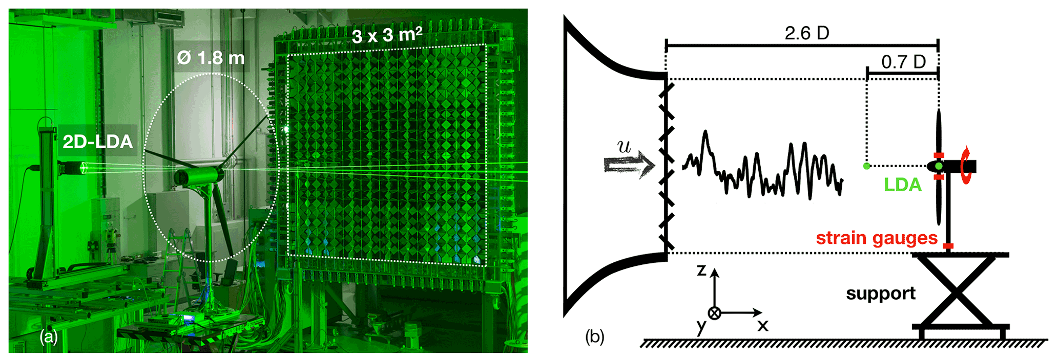
Figure 1 (a) Picture of MoWiTO 1.8 and 2D-LDA in a wind tunnel with active grid. Note the visible shift of grid flap angles between the centred inner square and outer compensating axes, demonstrated in the picture for a smaller inner square part than used in the investigation. (b) Schematic of setup with coordinate system in the wind tunnel.

2.1 Experimental setup

2.1.1 Wind tunnel

The experiments were performed in the large wind tunnel of ForWind – University of Oldenburg. The Göttingen-type wind tunnel has an outlet section of 3 m by 3 m. The wind tunnel was operated in an open-jet test section configuration with a test section length of 30 m (maximum wind velocity of 32 m s⁻¹). The wind tunnel is described in more detail in Kröger et al. (2018).

2.1.2 Active grid

An active grid is attached to the wind tunnel nozzle to manipulate the flow (Kröger et al., 2018; Neuhaus et al., 2021). The grid consists of 80 individually controllable shafts with rectangular flaps to control the distribution of blockage of the flow. Thus, wind variations can be repeatedly generated, as shown by Kröger et al. (2018). The active grid is shown in Fig. 1a.

2.1.3 Model turbine

The Model Wind Turbine Oldenburg with a diameter (D) of 1.8 m (MoWiTO 1.8) is used for the investigation (see Fig. 1a). The turbine is aerodynamically scaled based on the NREL 5 MW reference turbine (Jonkman et al., 2009) and maintains the design tip speed ratio (TSR; 7.5), thrust and power characteristics, and the non-dimensional lift and thus induction distribution. The turbine blades are scaled by a geometrical factor of $n_{\mathrm{length}}=\frac{\mathrm{1}}{\mathrm{70}}$. Influenced by structural constraints, the time scaling of the design is n_time=50. This leads to n_time-times-faster rotor speeds, $\frac{\mathrm{1}}{n_{\mathrm{time}}}$-times-shorter gust length, and a factor of n_time⋅n_length on the wind velocity. Low Reynolds number profiles are used for the stiff carbon-fibre-made blades. The blades have an estimated maximum tip deflection of less than 0.015 m at the maximum wind velocity (8.6 m s⁻¹) in this study and a first eigenfrequency of 32 Hz. The turbine has no rotor tilt or blade coning. It features individual pitch motors, torque control, and encoders for rotor rotation and position. Further, strain gauges for flapwise blade root bending moment, rotor torque and tower bottom bending moment (to derive the rotor thrust) are used. The turbine position in the wind tunnel is shown in Fig. 1b. Along the distance of 2.6 D behind the wind tunnel nozzle, the induction zone of the turbine can freely develop (see Medici et al., 2011). The turbine control and data acquisition are handled by a National Instruments CompactRIO system. The turbine scaling and design are described in detail in Berger et al. (2018).

2.1.4 Laser Doppler anemometer

A 2D laser Doppler anemometer (LDA) by TSI Inc., with a beam expander with a focus length of 2.1 m, is used. The optical measurement device is placed well outside of the wind flow. It is mounted on a motor-driven three-directional traverse with 1.5 m travel distance in each direction (see Fig. 1a). A LDA has no fixed sampling frequency but depends on various parameters, including the seeding of the wind flow with small oil particles. Typical LDA sampling frequencies in this experiment are 2 kHz.

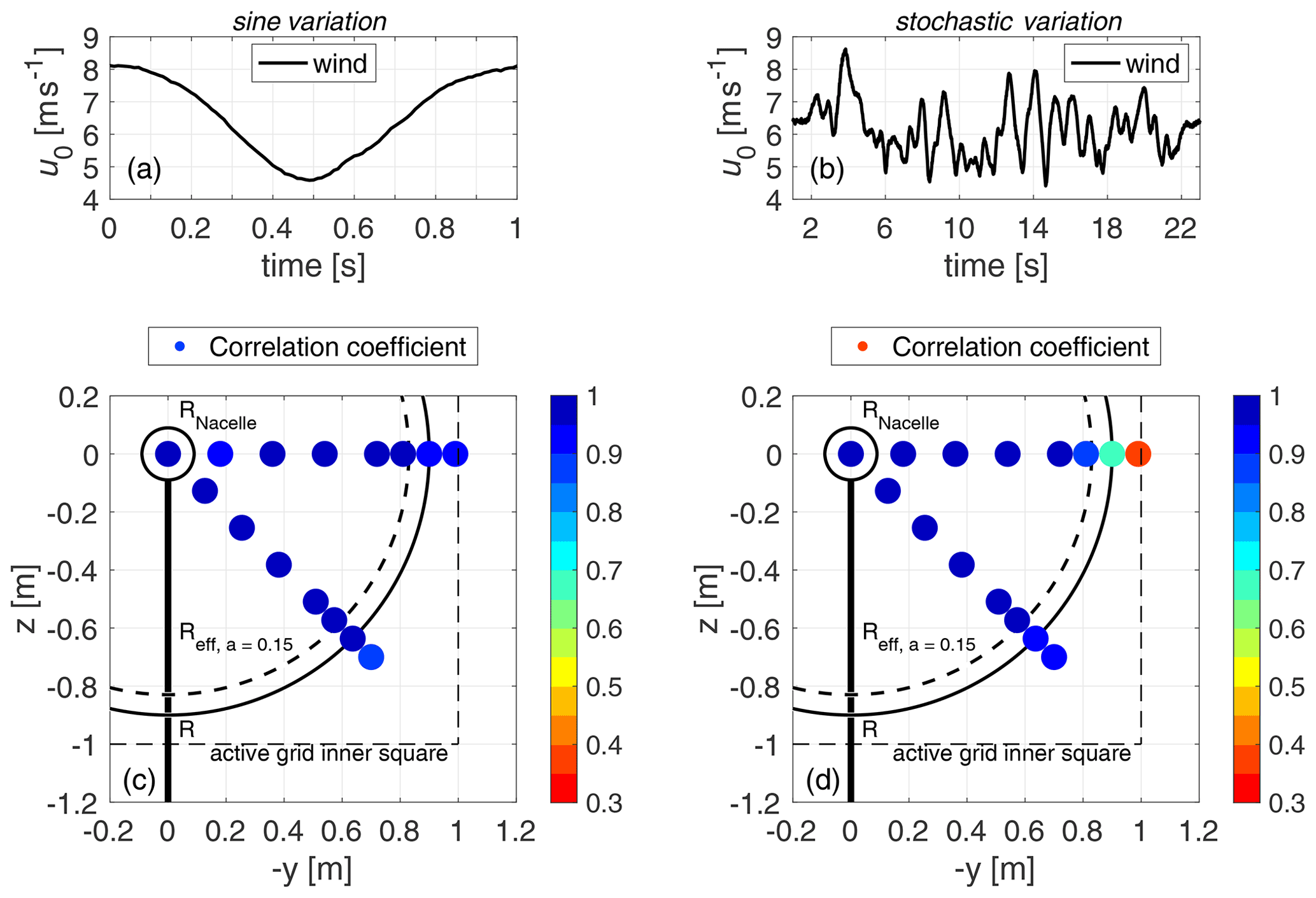
Figure 2 Undisturbed mean wind field of the sine (a) and stochastic (b) variation. Front view on the lower-right-hand-side quarter of the swept area of the turbine looking downstream. The colour-coded measurement positions show the Pearson correlation coefficient of the local measurement position wind velocity to the mean wind velocity for the sine (c) and stochastic (d) variation.

2.2 Wind fields

In this research the active grid is controlled by an overall constant blockage approach, where the inner square part (2 m by 2 m) of the grid impresses the desired gust conditions. The outer axes are used to keep the mean blockage of the grid constant. This way, fast velocity fluctuations with a high amplitude and degree of coherence can be achieved (Neuhaus et al., 2021). Two different types of transient wind fields with a high coherence over the swept area of the turbine are designed for this study. The wind tunnel fans are operated at constant speed, and the velocity patterns are impressed by the flaps of the active grid. The first wind field is based on a continuous sinusoidal wind velocity variation (sine) with a frequency of 1 Hz, mean wind velocity of 6.4 m s⁻¹ and an amplitude of 1.8 m s⁻¹. The second wind field has effectively 20 s of stochastic variations (stochastic), with a mean wind velocity of 6.2 m s⁻¹, maximum value of 8.6 m s⁻¹ and minimum value of 4.4 m s⁻¹.

The wind fields are quantified based on LDA measurements at 15 positions 0.7 D upstream of the turbine at standstill. The streamwise position of the measurements is indicated in Fig. 1b. The positions are located in a y–z plane (parallel to rotor plane). We measure on a horizontal (−y direction) and diagonal line (−y and −z direction) starting from the centreline of the wind tunnel in steps of 0.2 to 0.8 R and finer step width of 0.1 R from 0.8 to 1.1 R, where R is half of the rotor diameter D. Due to the symmetry of the square grid, the measurement points within the considered quarter of the rotor give a good representation of the whole swept area. For the sine variation 40 repetitions are considered, and for the stochastic variation 10 repetitions per position are considered.

These measurements are synchronised with the grid movement. For each wind field, a spatial mean wind velocity is defined by firstly binning all time series of the positions up to 0.9 R from the rotor axis to bins of 0.01 s and then averaging each bin. This gives a 100 Hz sampled spatial mean wind signal, as shown in Fig. 2a and b.

The level of uniformity over the swept area is assessed based on the Pearson correlation coefficient, as a measure of correlation of the wind velocity at single positions to the mean wind signal. It is calculated for the separately binned and averaged different positions in comparison to the spatial mean wind signal. These values are plotted colour coded at the measurement positions alongside relevant turbine dimensions in Fig. 2c and d. Additionally, a local stream-tube radius (R_eff) is plotted that takes into account the widening of the stream tube due to the induction zone at a rotor-averaged axial induction of a=0.15 for the running turbine.

Correlation coefficients within the local stream-tube radius are very high for both wind fields and for the sine variation for all measured positions, as expected based on the investigation by Neuhaus et al. (2021). For the stochastic variation the correlation decreases towards the edge of the active grid inner square, with still high values within R_eff. The level of uniformity over the rotor swept area is evaluated as sufficient for the planned investigation. In the later analyses, 95 % CIs (confidence intervals) are determined for various measured quantities. They are based on the binned data of all measurements within R_eff.

Cross-correlation between the mean velocity 0.7 D upstream of the turbine and the spatial mean velocity of three standstill (locked rotor) measurements in the rotor plane (0.4, 0.6 and 0.8 R) is used to obtain the time delay the wind field needs to reach the turbine from the upstream characterisation point. This time delay is needed later to align the dynamic and quasi-steady measurement signals. Comparing the measurements 0.7 D upstream of the turbine and in the rotor plane, we only see minor differences between signals. To account for possible small changes in the wind field while travelling from 0.7 D upstream of the turbine to the rotor plane, the uncertainty band will be altered in later analyses at few single instances, in order to always encase the spatial mean velocity measured in the rotor plane.

2.3 Measurement matrix

Aerodynamic rotor torque, thrust and flapwise blade root bending moments are obtained based on strain gauge measurements.

Additionally to the two wind fields, a staircase variation with 12 steps with a length of 25 s each and velocity range from 4.6 to 9.0 m s⁻¹ is performed for a turbine characterisation. For this wind field, the speed of the wind tunnel fans is changed, and the grid flaps are at the constant open position, acting as a passive grid. The turbine is operated at a steady rotational speed of 480 min⁻¹ and a constant pitch setting of 1^∘ (towards feather) for all measurements with operating turbine.

The staircase wind field is characterised at five horizontal positions between 0.1 and 0.9 R at 0.7 D upstream of the turbine. LDA measurements of the streamwise velocity are performed in the rotor plane at nine radial (along x axis) positions (for the range 0.3 to 0.9 R in steps of 0.1 R and additionally at 0.25 and 0.95 R) for the operational sine and staircase variation. An overview of the test matrix with additional information on the repetitions for each wind field is given in Table 1.

Table 1 Experimental test cases including number of measurement positions of the LDA and repetitions.

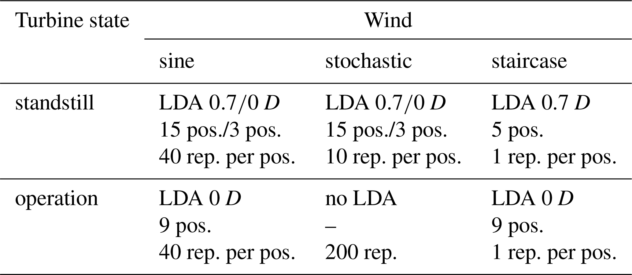
pos. = position; rep. = repetition.

2.4 Wake inductions

2.4.1 Measurement

The method by Herráez et al. (2018) is used to derive the wake induction factors. These are equal to the induction factors of a ring of an actuator disk and do not consider the induction contribution from the individual blades. The method is derived based on the theorem of Biot–Savart. For axial and uniform flow, the rotor blades have identical loading and circulation distribution at all azimuth positions. The velocity is probed in the bisectrix of two blades. Each blade's influence on the induced velocity due to its bound circulation is counterbalanced and thus cancels out, apart from the tip and root region due to the tip and root vortex, respectively. For the main part of the blade, however, Herráez et al. (2018) demonstrate the good applicability to derive the actual angle-of-attack distribution and thus velocity triangles at the blade segments from the measurement-derived wake induction factors. The method was developed for steady operation; however, it was shown in a prior study in Berger et al. (2021a) to be also applicable to study the transient changes in induction factors, maintaining axial and uniform conditions.

In Fig. 3a the turbine is shown with the LDA laser beams and the probed axial (u_ax) and tangential (u_ta) velocity components at a specific radius. In Fig. 3b the concept of the counterbalanced bound circulation of the evenly loaded blades is sketched. At the indicated line of measurement, the downwash of the blade ahead of the indicated line counteracts the upwash of the blade behind it, and they cancel each other out. The blade at the 9 o'clock position has no influence on the measurement. Herráez et al. (2018) outline that the trailed vorticity cannot be captured well due to the high distance between the measurement position and the blade tip. Therefore, this method is less suited for the root and tip region of the blade. The results at 0.25 and 0.95 R should therefore be interpreted with care. The application of this method with the same 2D LDA setup on MoWiTO is presented in detail and validated for an axial velocity probe over all azimuth angles at operation near design conditions in Berger et al. (2021a) (Sect. 2.1.3 and Appendix A). The same threshold value for the bisectrix position of the rotor azimuth angle of ±3^∘ was applied, as this was shown to be a good compromise between data samples and quality.

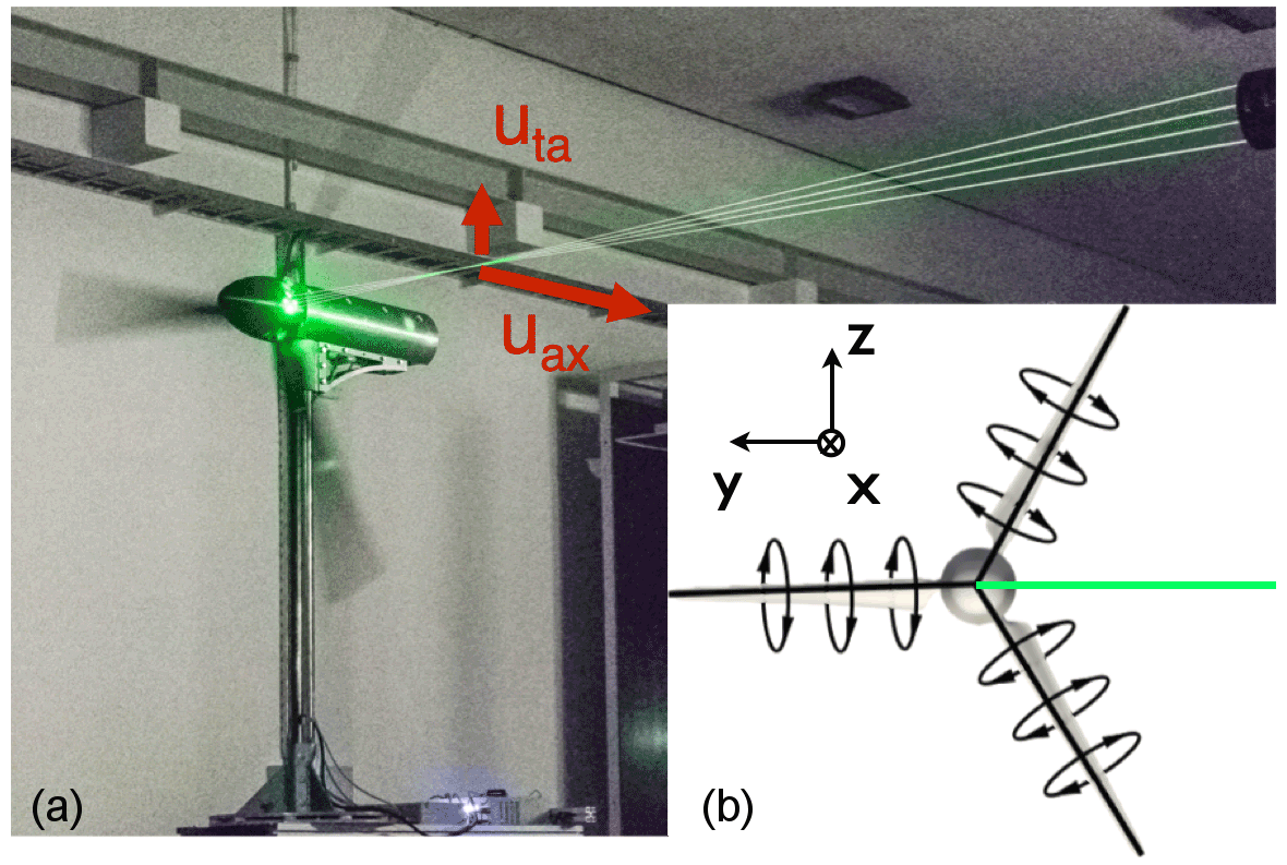
Figure 3 (a) MoWiTO 1.8 with 2D-LDA measurement in the bisectrix of two blades of axial and tangential velocity. (b) Counterbalancing of bound circulation for the evenly loaded blades (modified from Herráez et al., 2018).

The axial and tangential wake induction factors are defined by Eqs. (1) and (2), respectively. The undisturbed inflow velocity is u₀ and the rotor angular velocity Ω. With the geometrical angle of the blade segment γ, consisting of twist and pitch, the local angle of attack α at radius r can be calculated by Eq. (3).

$$\begin{array}{}\text{(1)}& {\displaystyle }& {\displaystyle }a=\mathrm{1}-{\displaystyle \frac{u_{\mathrm{ax}}}{u_{\mathrm{0}}}}\text{(2)}& {\displaystyle }& {\displaystyle }{a}^{\prime }={\displaystyle \frac{u_{\mathrm{ta}}}{\mathrm{\Omega }\cdot r}}\text{(3)}& {\displaystyle }& {\displaystyle }\mathit{\alpha }=\arctan \left({\displaystyle \frac{u_{\mathrm{ax}}}{u_{\mathrm{ta}}+\mathrm{\Omega }\cdot r}}\right)-\mathit{\gamma }\end{array}$$

2.4.2 Load reconstruction from inductions

The measurements of u_ax and u_ta are further used to reconstruct the turbine loads. The approach is based on the blade element theory (BET), usually used within a BEM code as outlined in detail by Hansen (2008) to obtain the aerodynamic forces from the flow information. The relative velocity at the blade segments is defined by Eq. (4). The angle of attack along the span is derived from the experiment through Eq. (3). The aerodynamic forces for single blade elements are calculated in the normal direction (F_N) by Eq. (7) and in the tangential direction (F_T) by Eq. (8). The inflow angle is the sum of α and γ and defined by θ. The lift and drag forces of the segment are given by Eqs. (5) and (6), respectively.

$$\begin{array}{}\text{(4)}& {\displaystyle }& {\displaystyle }{u}_{\mathrm{rel}}=\sqrt{u_{\mathrm{ax}}^{\mathrm{2}}+{\left(u_{\mathrm{ta}}+\mathrm{\Omega }r\right)}^{\mathrm{2}}}\text{(5)}& {\displaystyle }& {\displaystyle }{F}_{\mathrm{L}}={\displaystyle \frac{\mathrm{1}}{\mathrm{2}}}\cdot C_{\mathrm{L}}\left(\mathit{\alpha }\right)\cdot \mathit{\rho }\cdot \mathrm{\Delta }r\cdot c\cdot u_{\mathrm{rel}}^{\mathrm{2}}\cdot F\text{(6)}& {\displaystyle }& {\displaystyle }{F}_{\mathrm{D}}={\displaystyle \frac{\mathrm{1}}{\mathrm{2}}}\cdot C_{\mathrm{D}}\left(\mathit{\alpha }\right)\cdot \mathit{\rho }\cdot \mathrm{\Delta }r\cdot c\cdot u_{\mathrm{rel}}^{\mathrm{2}}\cdot F\text{(7)}& {\displaystyle }& {\displaystyle }{F}_{\mathrm{N}}=F_{\mathrm{L}}\cos \mathit{\theta }+F_{\mathrm{D}}\sin \mathit{\theta }\text{(8)}& {\displaystyle }& {\displaystyle }{F}_{\mathrm{T}}=F_{\mathrm{L}}\sin \mathit{\theta }-F_{\mathrm{D}}\cos \mathit{\theta }\end{array}$$

The lift and drag coefficients are given by C_L(α) and C_D(α), respectively, and obtained from XFoil (Drela, 1989) simulations for the respective Reynolds numbers. Three-dimensional effects are accounted for through the correction model for the lift coefficient at high angles of attack by Snel et al. (1993), which is mainly relevant for the root sections. The width of a blade segment is defined by Δr and the chord length by c. The tip losses are accounted for by the tip loss model by Shen et al. (2005) with the factor F. The segmented aerodynamic loads are integrated along the blade span to obtain the integral load signals.

2.5 Dynamic and quasi-steady cases

The dynamic and quasi-steady case during a gust is compared for different load and rotor flow signals. The difference between both cases results from the dynamic inflow effect. The dynamic measurement is denoted as the dynamic case. The quasi-steady case is the respective signal during the same gust without dynamic effects. They are interpolated from lookup tables based on the instantaneous gust wind speed. These lookup tables are based on a quasi-steady characterisation experiment. The processing of both the dynamic and quasi-steady signals is introduced in this subsection.

2.5.1 Dynamic experiment

Ensemble averages are calculated for each of the loads from the various repetitions of the two dynamic cases. For the sine gust the ensemble average of the flapwise blade root bending moment (M_flap) is thus based on the N=360 repetitions of the sine movement, according to Eq. (9).

$$\begin{array}{}\text{(9)}& M_{\mathrm{flap}}\left(t\right)={\displaystyle \frac{\mathrm{1}}{N}}\sum _{i=\mathrm{1}}^N{M}_{\mathrm{flap},\mathrm{single}\mathrm{cycle},\mathrm{all}\mathrm{blades}}^{\left(i\right)}\left(t\right)\end{array}$$

With this approach, noise and non-deterministic variations can be reduced. Even some deterministic fluctuations, like the blade–tower interaction, are smoothed out as the start of the active grid wind protocols and the rotor azimuth position are not synchronised.

The LDA-based induction measurement data for the sine variation are processed with a similar approach. The data points within the threshold in the bisectrix of the single repetitions are synchronised with the wind field and combined to one single signal. As the rotational frequency of 8 Hz of the rotor is a multiple of the frequency of the sine at 1 Hz, there are 24 data point clusters for this three-bladed turbine over one sine period (in Sect. 3.2.1 and Fig. 9a to c). These data are binned to clusters, and the mean value of each bin is taken as a representative value.

Corrections are applied to the torque and thrust signals based on the strain gauge measurements. To obtain the aerodynamic rotor torque, the measurement signal is corrected for two effects. Firstly, the friction in the main shaft bearings and slip ring is added to the measured torque. This correction increases the torque by 3 % at the mean velocity of the wind fields. Secondly, there is an inertial effect of the rotor due to slight changes in the rotor speed up to ±3 %, as the controller cannot keep the rotor perfectly constant for the fast changes in wind velocity. Equation (10) is used to correct the torque signal by the contribution ΔM(t) associated with the angular acceleration of the rotor $\dot{\mathrm{\Omega }}$ and inertia of the rotor and drivetrain I_rot.

$$\begin{array}{}\text{(10)}& \mathrm{\Delta }M\left(t\right)=I_{\mathrm{rot}}\cdot \dot{\mathrm{\Omega }}\left(t\right)\end{array}$$

As introduced, dynamic inflow effects can also be triggered by fast changes in rotor speed. The influence of the slight changes in rotor speed in the presented experiment are investigated with a BEM tool with the Øye dynamic inflow engineering model (see Sect. 2.6). As a result the influence of the dynamic inflow effect due to the rotor speed changes is considered negligible in the context of this work.

The thrust is derived from the tower bottom bending moment in fore–aft direction. The measurement is corrected for the influence of tower and nacelle drag. This drag was estimated based on a quadratic fit to a measurement of the tower bottom bending moment at various wind speeds with the turbine without installed blades.

2.5.2 Quasi-steady behaviour

Quasi-steady turbine loads and rotor flow are obtained based on linear interpolation from non-dimensional lookup tables for a range of TSR and dimensionalised again. These lookup tables are based on a detailed characterisation of the turbine with the staircase wind protocol. The uncommon blade root bending moment coefficient C_flap is defined in Eq. (11). The reference bending moment is the denominator of the thrust coefficient multiplied with an additional characteristic length of $\frac{\mathrm{2}}{\mathrm{3}}R$, based on the representative attack point of the load for an idealised triangular normal force distribution, and the reciprocal of the number of blades n_b. C_flap and the common thrust coefficient C_T and torque moment coefficient C_M are presented over TSR in Fig. 4.

$$\begin{array}{}\text{(11)}& C_{\mathrm{flap}}={\displaystyle \frac{n_{\mathrm{b}}{M}_{\mathrm{flap}}}{\frac{\mathit{\rho }}{\mathrm{2}}{u}_{\mathrm{0}}^{\mathrm{2}}\mathit{\pi }{R}^{\mathrm{2}}\frac{\mathrm{2}}{\mathrm{3}}R}}\end{array}$$

Error bars indicate the quadratically added up uncertainty of inflow wind velocity and the 95 % CI of the load measurement for the 20 s long considered measurement length per wind velocity step. The additional plus sign represents an extrapolated value slightly outside of the staircase wind protocol. This extra value is needed to construct the quasi-steady loads at a single negative wind gust for the stochastic wind variation case.

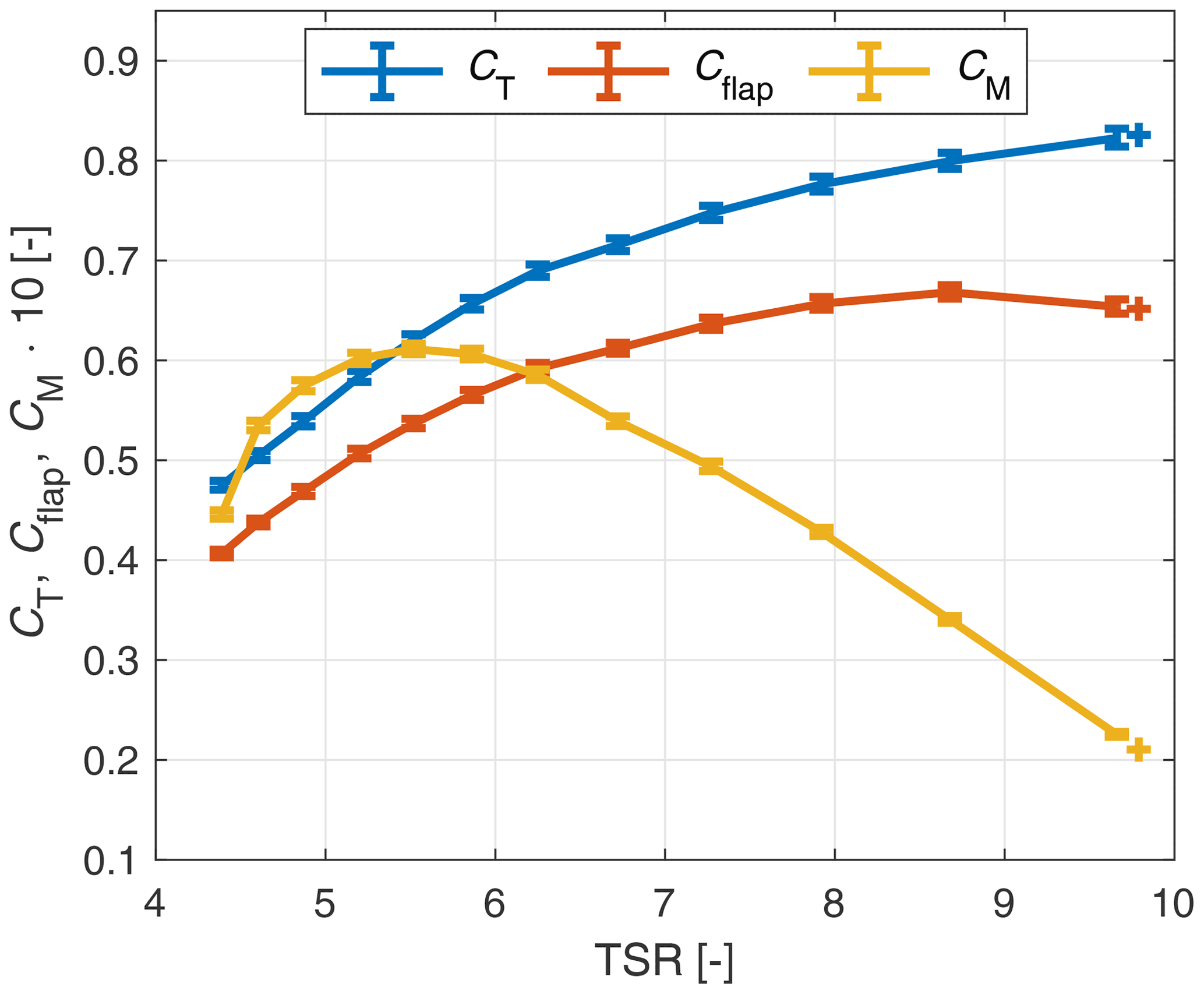
Figure 4 Turbine characteristics for construction of the quasi-steady case. Relevant TSR range for the sine and stochastic wind variation is TSR 5.6 to 9.5 and 5.4 to 9.8, respectively.

The axial (see Eq. 1) and tangential (see Eq. 2)) induction factors are obtained with the same staircase wind protocol. Based on these also the angle of attack (see Eq. 3) is obtained. The lookup tables for the quasi-steady rotor flow are constructed for the nine considered radii and nine different TSR values (in TSR range 5.6 to 9.5). For clarity only three representative measured distributions over radius are shown in Fig. 5a–c.

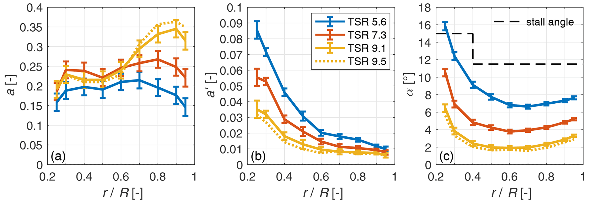
Figure 5 Distributions of (a) axial induction factor, (b) tangential induction factor and (c) angle of attack for different TSR. The dotted line represents a linear extrapolation.

The solid lines represent the highest, lowest and middle operational TSR configurations for the needed range of the sine case within the staircase characterisation. The error bars indicate the quadratic error of the inflow uncertainty and the 95 % CI of the induction measurement for the inductions and the propagated error for the angle of attack. Another high-TSR state is extrapolated and shown in dashed lines. This extrapolation, however, is only minor. At the highest TSR operational point in the characterisation, the rotor speed dropped due to the chosen controller settings. This led to a lower TSR value than needed for the construction of the quasi-steady signals. For the load characterisation, additional characterisations at higher rotor speed were recorded. Therefore, the highest recorded TSR in the characterisations of loads and inductions differs.

The trends for the axial and tangential induction and angle of attack are as expected. The axial induction factor (Fig. 5a) for the low and middle TSR setting shows a uniform spanwise distribution. We see higher values of a for higher TSR. For the high-TSR settings these values in the inner rotor half decrease again, whereas the axial induction factor is increased in the outer rotor half, compared to the TSR 7.3 case. Axial induction factors are below the design induction factor for optimal power extraction of $\mathrm{1}/\mathrm{3}$, apart from the tip region at the high-TSR settings where the maximum value is found at 0.36. Thus, the turbine is not operating within the turbulent wake state throughout the experiments, as can also be seen at the maximum C_T value of 0.83.

The tangential induction factor (Fig. 5b) has high values near the root, which decrease towards the outer part. Also, the tangential induction values generally decrease with increasing TSR for the respective radii, as expected from the decreasing momentum coefficient from the low to high TSR (see Fig. 4).

The angle of attack (Fig. 5c) is higher towards the root and similar for the range from 0.5 R to the tip. The general distributions show the highest radius-dependent angles of attack for the low-TSR setting and decrease with increasing TSR. The stall angle is estimated to be at the highest lift coefficient at 15^∘ for the root airfoil up to 0.4 R and at 11.5^∘ for the airfoil used from 0.5 R to the tip. This limit is exceeded at the lowest TSR setting for the radius at 0.25 R. For the remaining radii at this TSR and higher TSR in general, the angles of attack are within the stall limits.

The quasi-steady turbine loads and inductions, lacking the dynamic inflow effects, are obtained for the dynamic wind field by interpolation from this characterisation. The reference wind speed of the gust at the rotor plane position is used for the construction. This reference speed is the mean of the measured 15 positions in front of the turbine, and a time delay was obtained based on minimising the root mean square error in the cross-correlation of the mean wind to the mean velocity of the three reference wind measurements in the rotor plane.

2.6 Øye dynamic inflow model and improved formulation for gusts

In BEM simulations, engineering models are needed to catch the dynamic inflow effect. By filtering the induced velocity, the inertia of the wake is considered, leading to a load overshoot for a sudden change in rotor load, e.g. by a fast pitch step.

The dynamic inflow effect due to a pitch step should be described by two time constants (Pirrung and Madsen, 2018; Yu et al., 2019; Berger et al., 2021a). The faster time constant τ_fast can be attributed to the sudden change in the trailed vorticity near the rotor plane and has relevant radial dependency. When that change in trailed vorticity is convected downstream with the wake, it has a more global effect and slower rate of change, described by the slower time constant τ_slow with little radial dependency.

A gust can also lead to fast changes in u_ind within relevant timescales to the dynamic inflow effect (${\mathit{\tau }}_{\mathrm{typ}}=R/u_{\mathrm{0}}$, see Snel and Schepers, 1994). Such gust cases differ physically from the more classic dynamic inflow cases of a fast pitch step or rotor speed change. Considering a turbine model without any dynamic effects at constant rotational speed, a fast increase in u₀ due to a gust leads to a decrease in a (due to the reduced TSR). With the induced velocity being $u_{\mathrm{ind}}=a\cdot u_{\mathrm{0}}$, the effect of increase in u₀ on u_ind is partly compensated for by the decrease in a. Therefore, the dynamic inflow effect is expected to be less significant than for a pitch step (only changes a), as outlined in Snel and Schepers (1994).

In the following are the formulations of the Øye dynamic inflow model and a suggested improvement to the model.

2.6.1 Øye model

In the Øye dynamic inflow model the steady induced velocities are filtered through two first-order differential equations as in Eqs. (12) and (13) (Snel and Schepers, 1994; Hansen, 2008).

$$\begin{array}{}\text{(12)}& {\displaystyle }\begin{array}{rl}{u}_{\mathrm{ind},\mathrm{int}}\left(t\right)& +{\mathit{\tau }}_{\mathrm{slow}}{\displaystyle \frac{\mathrm{d}{u}_{\mathrm{ind},\mathrm{int}}\left(t\right)}{\mathrm{d}t}}=u_{\mathrm{ind},\mathrm{qs}}\left(t\right)+k\\ & \cdot {\mathit{\tau }}_{\mathrm{slow}}{\displaystyle \frac{\mathrm{d}{u}_{\mathrm{ind},\mathrm{qs}}\left(t\right)}{\mathrm{d}t}}\end{array}\text{(13)}& {\displaystyle }{u}_{\mathrm{ind}}\left(t\right)+{\mathit{\tau }}_{\mathrm{fast}}{\displaystyle \frac{\mathrm{d}{u}_{\mathrm{ind}}\left(t\right)}{\mathrm{d}t}}=u_{\mathrm{ind},\mathrm{int}}\left(t\right)\end{array}$$

u_ind,qs is the quasi-steady induced velocity, u_ind,int is an intermediate and u_ind is the final filtered induced velocity. The time constants τ_slow and τ_fast are defined by Eqs. (14) and (15), respectively, and their weighting ratio k by Eq. (16).

$$\begin{array}{}\text{(14)}& {\displaystyle }& {\displaystyle }{\mathit{\tau }}_{\mathrm{slow}}={\displaystyle \frac{\mathrm{1.1}}{(\mathrm{1}-\mathrm{1.3}a)}}{\displaystyle \frac{R}{u_{\mathrm{0}}\left(t\right)}}\text{(15)}& {\displaystyle }& {\displaystyle }{\mathit{\tau }}_{\mathrm{fast}}=\left[\mathrm{0.39}-\mathrm{0.26}{\left({\displaystyle \frac{r}{R}}\right)}^{\mathrm{2}}\right]{\mathit{\tau }}_{\mathrm{slow}}\text{(16)}& {\displaystyle }& {\displaystyle }k=\mathrm{0.6}\end{array}$$

2.6.2 Improved formulation of Øye model for gusts

The Øye model is developed for the assumption of constant wind velocity and filters the induced velocity through two first-order differential equations. In Schepers (2007) the dynamic inflow effect is described for a fast change in thrust alongside the reproduced Fig. 6a. The trailed vorticity is formed at the blade and convected with the total local velocity, which is in parts induced by the wake. A change in bound vorticity through a pitch step modifies that vorticity, trailed into the wake. Due to the convection with a finite velocity, a mixed wake forms that consists of “old” and “new” vorticity. This mixed wake influences then the induced velocities.

Figure 6 Wake with mixed vorticity as a result of a fast change in thrust (modified from Schepers, 2007) (a) and simplified turbulent box with coherent gust-like sudden drop in wind velocity (b).

Schepers (2007) estimates that the effect of this mixed wake influences the rotor flow until it has travelled 2 to 4 D, before the induced velocity has reached a new equilibrium. In Berger et al. (2021a) a relevant distance of 2 D is estimated based on a comparison of wake measurements and dynamic turbine loads.

In Fig. 6b a coherent gust, in this case a rapid decrease in wind velocity, is sketched as a turbulent box with only one grid point. When this box is pushed through the wind turbine above (e.g. with the mean wind velocity of the seed as is done in BEM and FVWM simulations) in Fig. 6a, it also causes a change in bound vorticity that is trailed into the wake. This is covered by the original Øye model.

However, the wake with the old and new vorticity is convected by the local wind velocity, partly wake induced. For the shown case, this local wind velocity in the relevant wake distance is in parts higher than in the rotor plane. The wake is convected faster than in the assumption for the Øye model. This effect is expected to increase the axial velocity as additional air volume is pulled through the rotor by the inertia of the wake. This increases the angle of attack during the step change to lower wind velocity and thus leads to a more gradual change in the turbine load.

To include this effect in the dynamic inflow model, an additional time derivative on the undisturbed wind velocity u₀(t) is added to the computation of the intermediate induced velocity (u_ind,int(t)) in the Øye dynamic inflow model to the right-hand side of Eq. (12), which is then written as Eq. (17). With this extra term ($k_u\cdot {\mathit{\tau }}_{\mathrm{slow}}\frac{\mathrm{d}{u}_{\mathrm{0}}\left(t\right)}{\mathrm{d}t}$) any change in wind velocity drives the time filter of u_ind,int(t). For constant wind velocity, the extra term has no impact and the model is essentially the original Øye dynamic inflow model.

$$\begin{array}{}\text{(17)}& \begin{array}{rl}{u}_{\mathrm{ind},\mathrm{int}}\left(t\right)& +{\mathit{\tau }}_{\mathrm{slow}}{\displaystyle \frac{\mathrm{d}{u}_{\mathrm{ind},\mathrm{int}}\left(t\right)}{\mathrm{d}t}}=u_{\mathrm{ind},\mathrm{qs}}\left(t\right)\\ & +\cdot {\mathit{\tau }}_{\mathrm{slow}}\left(k\cdot {\displaystyle \frac{\mathrm{d}{u}_{\mathrm{ind},\mathrm{qs}}\left(t\right)}{\mathrm{d}t}}+k_u\cdot {\displaystyle \frac{\mathrm{d}{u}_{\mathrm{0}}\left(t\right)}{\mathrm{d}t}}\right)\end{array}\end{array}$$

A good initial fit to the experiment was found with the slow time constant τ_slow and the factor k_u=0.2.

2.7 Comparing simulations

Two different kinds of simulations, a BEM and a FVWM based, are used for comparison with the experimental data. For the BEM simulation the dynamic inflow engineering model is disabled to get the steady case. For the FVWM the quasi-steady cases are generated similar to the experiment. A lookup table with relevant quantities is generated based on a staircase wind input, and the quasi-steady case is obtained from linear interpolation by the respective wind field. The same airfoil polars as in Sect. 2.4.2 are used.

The first simulation environment is a BEM model programmed in MATLAB and based on Hansen (2008). The BEM program considers axial and uniform inflow, considers equal loading for all blades, and features a Shen tip loss model and high thrust correction (Buhl, 2005). The Øye dynamic inflow engineering model and the improved version for gusts (see Sect. 2.6) are implemented.

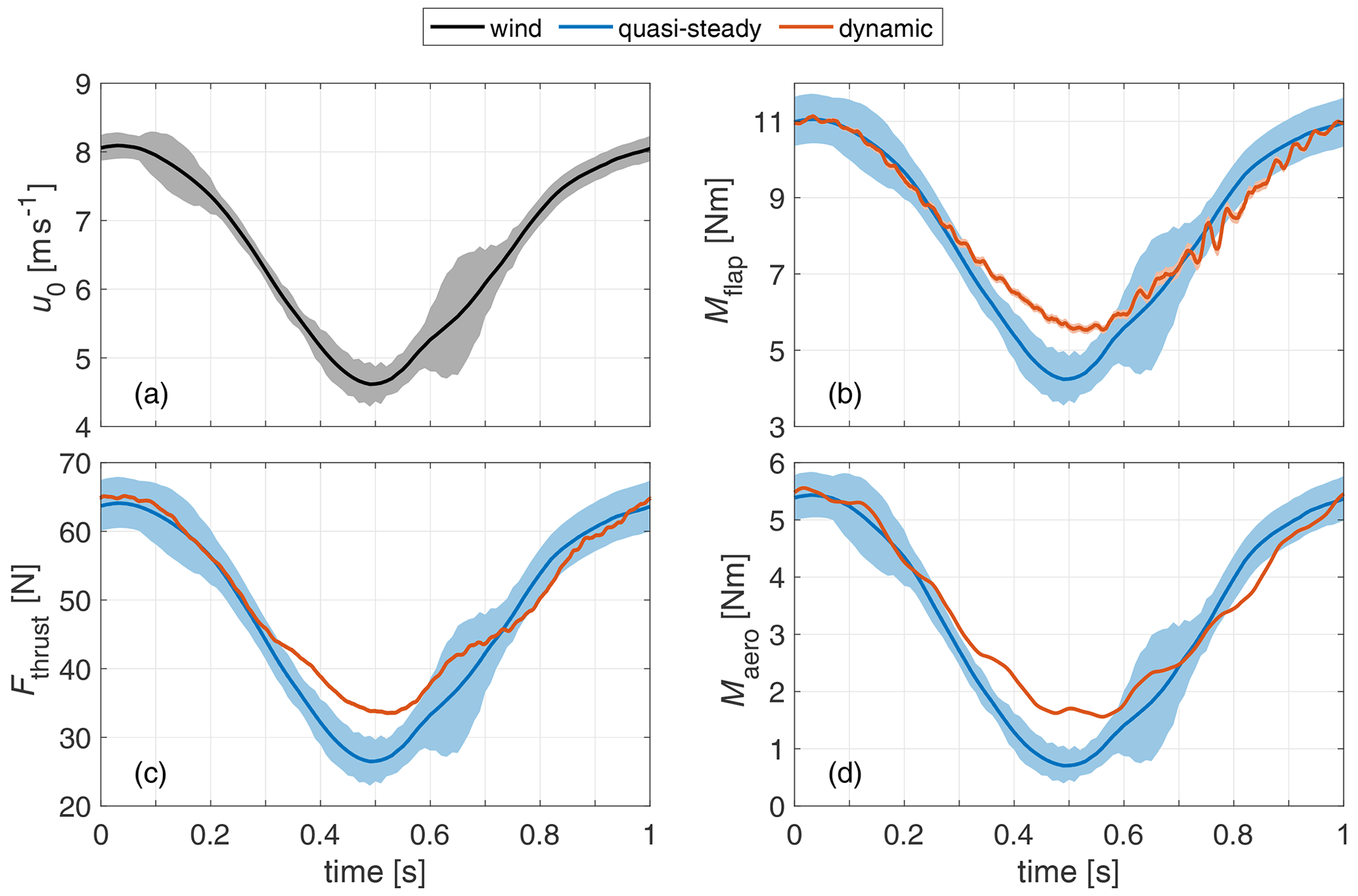
Figure 7 Sine wind field (a) and quasi-steady and dynamic experiment loads for flapwise blade root bending moment (b), thrust (c) and aerodynamic torque (d). The wind uncertainty shows the degree of uniformity. The uncertainty for the quasi-steady loads accounts for this non-uniformity and the uncertainty in the aerodynamic characterisation. The dynamic loads are shown along the 95 % CI.

The second simulation environment is the FVWM model implemented in QBlade (Marten et al., 2016). It is based on the principles of Van Garrel (2003). The flow field is modelled as a potential flow. The MoWiTO blade is discretised in 15 elements, which are each modelled by a bound ring vortex, thus forming a lifting line. The circulation of these vortices is calculated iteratively based on the airfoil polars and relative velocity. The vorticity is shed and trailed at each time step. The wake convection is obtained by forward integration with a first-order method. A turbulent wind field is handled as a turbulent box that is moved through the wind turbine domain with the hub height mean wind velocity of the turbulence seed. The turbulent wind field is also used for the convection of the wake vortices. The induced velocity is influenced by the physical representation of the convecting wake, thus intrinsically modelling the dynamic inflow effect. The wake of 12 revolutions is considered, and the azimuthal discretisation is 10^∘.

Both model setups were already used in Berger et al. (2020) and showed a good match to an experimental dynamic inflow focused pitch step experiment (Berger et al., 2021a) with MoWiTO. For both models neither unsteady profile aerodynamics nor structural flexibility are considered, but only the aerodynamic degrees of freedom at constant rotation.

3 Results

At first, the integral loads for sine and stochastic wind fields are presented, comparing the quasi-steady experiment and dynamic experiment. Next, the radially resolved axial velocity and induced velocity of the sine gust is investigated. The thrust force is reconstructed based on these induction measurements. Lastly, a comparison of thrust and induced velocity for the sine gust of BEM and FVWM simulations to the experiment is presented.

3.1 Loads

3.1.1 Sine inflow variation

In Fig. 7, the sine wind field (Fig. 7a) and loads for flapwise blade root bending moment M_flap (Fig. 7b), thrust F_thrust (Fig. 7c), and aerodynamic rotor torque M_aero (Fig. 7d) of the quasi-steady experiment case and dynamic experiment case are plotted over time. The uncertainty band around the wind field shows the 95 % CI of the sine wind field altered to higher error at few positions to enclose the mean wind vector based on the three standstill measurements in the rotor plane (see Sect. 2.2). These alterations are mainly in the range t=0.1 to t=0.2 s and t=0.6 to t=0.7 s. The uncertainty band around the quasi-steady loads accounts for the quadratically added uncertainty in the wind velocity and the estimated error in the load characterisation (see Fig. 4). The uncertainty of the dynamic experiment shows the 95 % CI of the load measurement.

In the comparison of the quasi-steady case with the experiment case, the three considered load channels show similar behaviour. At the positive gust peak at t=0 s, the steady case and experiment case show similar values, but they differ at the negative gust peak at t=0.5 s. Here the experiment shows higher absolute loads than the quasi-steady case, thus leading to a reduction in load amplitude of the dynamic experiment by 20 % to 23 %, based on the amplitude of the quasi-steady case.

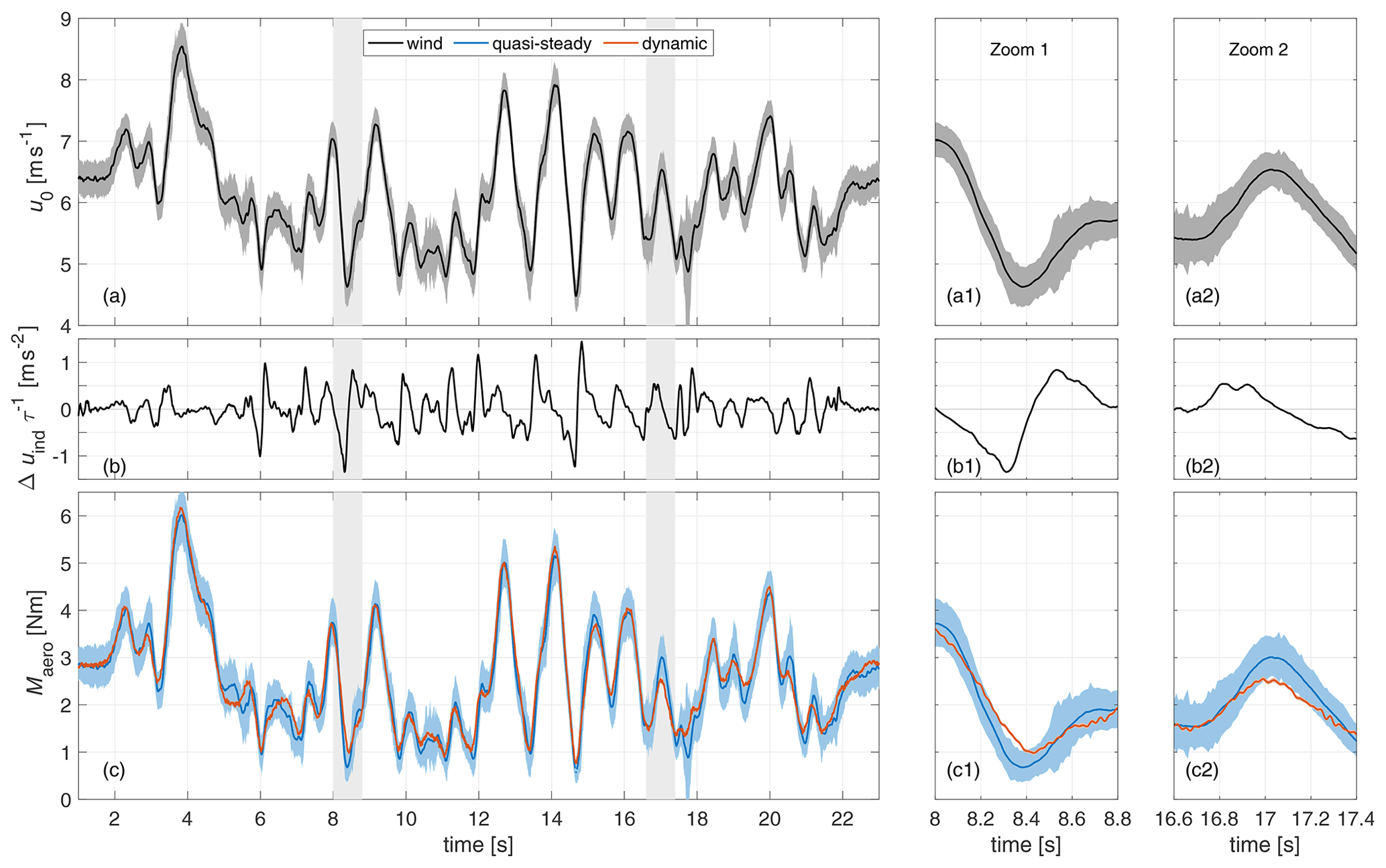
Figure 8 Stochastic wind variation (a), difference quotient of velocity with τ to obtain the instances of largest relevant velocity change (b), and flapwise blade root bending moment (c) for the steady case and dynamic case. Furthermore, two zoomed-in views (marked in grey in the whole time series) of situations of interest of the same data series are presented (a1, a2, b1, b2, c1, c2).

The steady and dynamic curves differ mainly for the range of t=0.3 to $t=\mathrm{0}.$6 s, where the wind velocity decreases quickly and the turbine operates at high TSR and thus thrust coefficients. The dynamic loads react with a reduced change in load from t=0.3 s on and reach the quasi-steady curve again after the wind velocity increases at t=0.6 s. For the torque, this behaviour can also be seen less pronounced for the increasing wind velocity slope around t=0.8 s.

3.1.2 Stochastic inflow variation

Figure 8 shows the wind velocity of the stochastic wind variation in Fig. 8a, the difference quotient of the rotor equivalent induced velocity to a relevant dynamic inflow time constant τ in Fig. 8b, and M_aero for the quasi-steady case and dynamic case in Fig. 8c. The uncertainty for the wind and M_aero(t) is shown as for the sine gust. The induced velocity is estimated based on the quasi-steady thrust coefficient via the momentum balance ($C_{\mathrm{T}}=\mathrm{4}a(a-\mathrm{1})$). The reference time constant ($\mathit{\tau }=\frac{\mathrm{1}}{\mathrm{2}}{\mathit{\tau }}_{\mathrm{typ}}$) was chosen to be half of the typical dynamic inflow value (${\mathit{\tau }}_{\mathrm{typ}}=\frac{R}{\stackrel{\mathrm{‾}}{u_{\mathrm{0}}}}$) as introduced in Schepers and Snel (1995)) for a simple evaluation of the dynamic inflow effect with a single time constant. This τ=0.07 s also equals the duration of the fast pitch step in Berger et al. (2021a) with MoWiTO, thus giving a relatable time frame for a change in turbine loading that can lead to a clear dynamic inflow effect with this similar MoWiTO setup. The typical time constant is also commonly used as a scaling parameter in two-time-constant dynamic inflow models as can be seen in Eq. (14). With the difference in induced velocity $\mathrm{\Delta }{u}_{\mathrm{ind}}\left(t\right)=u_{\mathrm{ind}}\left(t\right)-u_{\mathrm{ind}}(t-\mathit{\tau })$, the difference quotient is $\frac{\mathrm{\Delta }{u}_{\mathrm{ind}}\left(t\right)}{\mathit{\tau }}$. A high amount shows a fast change in induced velocity and thus indicates instances where dynamic inflow effects are to be expected based on current engineering models. Additionally, two zoomed-in views of interest, based on relevant differences between steady M_aero(t) and dynamic M_aero(t), are shown.

The comparison of the quasi-steady and dynamic M_aero(t) shows a good fit, with only two instances where the dynamic values are outside of the quasi-steady range. The first instance is shown in zoom 1. The wind velocity (Fig. 8a1) decreases quickly from t=8 s to t=8.4 s, and the dynamic torque (Fig. 8c1) shows a less pronounced response, similar to the negative gust for the sine variation. The difference quotient of the induced velocity (Fig. 8b1) shows the absolute minimum at t=8.3 s, coinciding with the maximum difference between experiment and quasi-steady case.

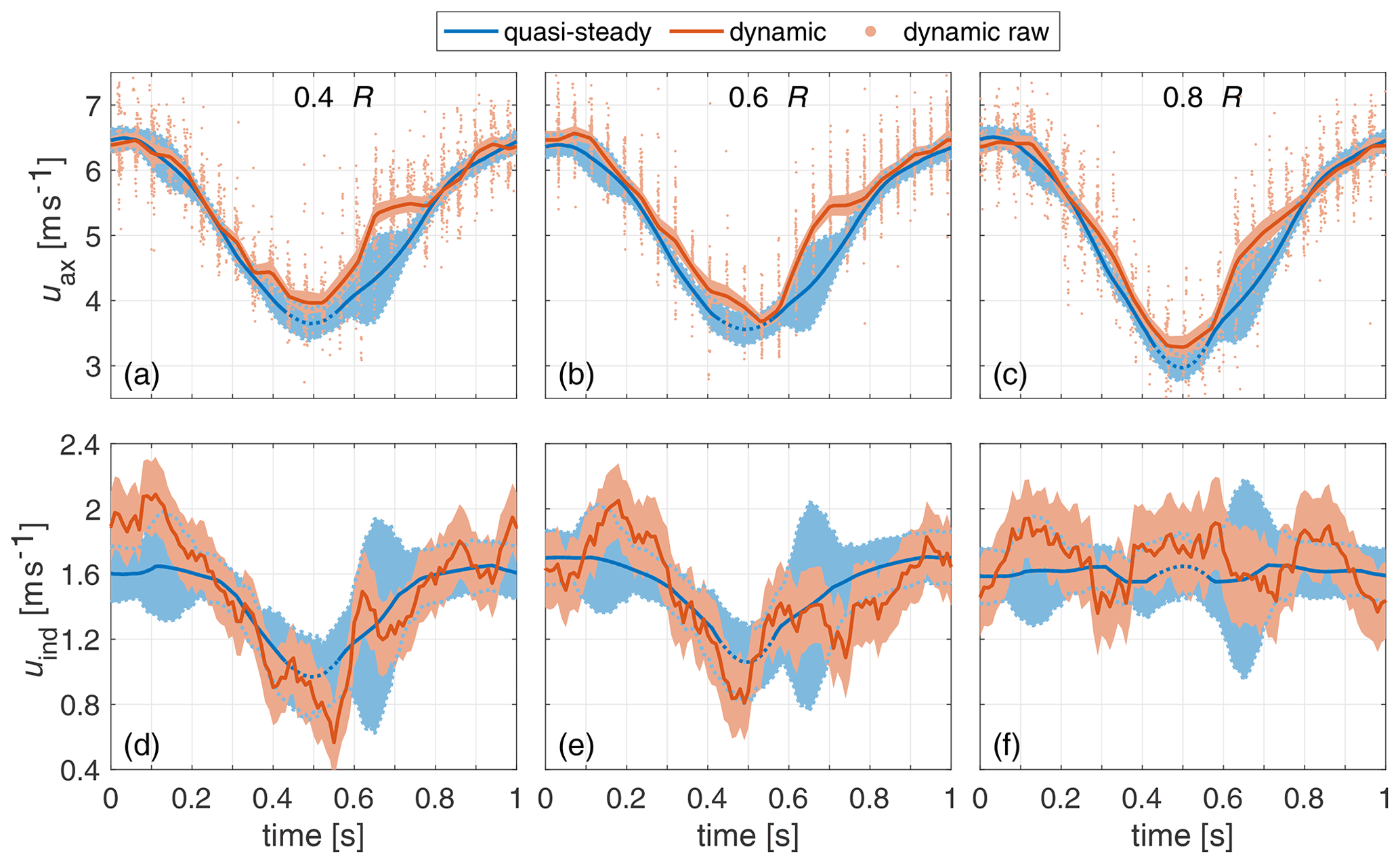
Figure 9 Quasi-steady and dynamic axial velocity and induced velocity for sine wind field at radii 0.4 R (a, d), 0.6 R (b, e) and 0.8 R (c, f). The 95 % CIs are given, and errors for the quasi-steady case and the induced velocity of the dynamic case were quadratically added. Note that the reference velocity values for the quasi-steady and dynamic induced velocity slightly differ.

The second instance is around t=17 s. There is a fast increase in wind velocity (Fig. 8a2), and the dynamic M_aero(t) (Fig. 8c2) does not increase as fast as for the quasi-steady case, thus leading to a less pronounced load peak for the dynamic case. The difference quotient of the induced velocity (Fig. 8b2), in contrast to Fig. 8b1, does not show an extreme value here. In general there is a slightly reduced variation of M_aero(t) of the dynamic case in comparison to the steady case, especially at the lower tipping points. Apart from the two introduced instances, these differences are all within the uncertainty range. For the two described instances, no extrapolated values were needed for the quasi-steady M_aero(t) signal.

3.2 Radially resolved measurement

For the sine wind field, quasi-steady and dynamic u_ax(t) and u_ind(t) are directly compared for three radii. In the next step all considered radii are used to reconstruct the rotor thrust based on the flow measurement (see Sect. 2.4.2). This way, the radial measurements are combined to a global signal, reducing uncertainty and noise.

3.2.1 Axial and induced velocity

In Fig. 9a–c, the axial velocity u_ax(t) values for three radii for the dynamic and quasi-steady cases for the sine wind field are shown. For the dynamic case the raw data samples are additionally plotted. The 95 % CI is given for both signals. For the quasi-steady case this is again altered by the mean wind velocity in the rotor plane at single instances. The dotted line for the quasi-steady case indicates the extrapolated range of the characterisation.

The steady and dynamic axial velocity shows similar behaviour for the three chosen radii. However, differences are evident at the lower tipping points. For all three radii the dynamic case shows higher u_ax(t) values here. At all radii but especially 0.4 and 0.6 R, a plateau can be seen in the dynamic case around t=0.7 s. This effect is also indicated in the uncertainty band of the quasi-steady case but not in the dynamic load measurements. This indicates a local flow pattern that is smoothed out globally.

In Fig. 9d–f, the induced velocity $u_{\mathrm{ind}}\left(t\right)=u_{\mathrm{0}}\left(t\right)-u_{\mathrm{ax}}\left(t\right)$ values for the steady case and dynamic case are plotted for the three radii. The reference velocity values for the steady case and dynamic case are the wind velocity u₀(t) as shown in Fig. 7a and the corresponding local in-plane standstill measurement u_0,local(t), respectively. The local reference velocity is used for a smoother representation of the sensitive induced velocity, as the local reference velocity also contains the described local flow patterns.

The quasi-steady values show a dip by 0.4 m s⁻¹ between t=0.3 and t=0.5 s for the radii 0.4 and 0.6 R. For 0.8 R the induced velocity is nearly constant for the whole sine wind variation.

In general the dynamic u_ind(t) has a high level of signal noise. This can be related on the one hand to the combination of small values for u_ind(t) and the noise in the signals u_0,local(t) and u_ax(t). On the other hand u_0,local(t) and u_ax(t) consider the same position; however, the effect of the widening stream tube around the rotor is not considered, leading to some possible mismatches in u_0,local(t). Still the comparison gives valuable insights in the phenomenon.

At 0.8 R the dynamic u_ind(t) does indicate a steady value but with a higher noise level. For the radius at 0.6 R, steady u_ind(t) and dynamic u_ind(t) start at the same level, whereas the dynamic u_ind(t) increases from t=0.1 to t=0.2 s and the quasi-steady signal stays levelled. In the further course the dynamic signal decreases quicker and further from t=0.3 to t=0.5 s below the quasi-steady value. From there, the dynamic u_ind(t) does increase to the steady value and again below it around t=0.7 s, before reaching the steady level again at the end of the sine wind variation. The 0.4 R case is similar, with the exception that the dynamic signal already starts at a higher value than the quasi-steady one. The differences between steady u_ind(t) and dynamic u_ind(t) are indications, as the uncertainty range of the quasi-steady case and experiment overlay. However, for some instances, e.g. for 0.4 R at t=0 to t=0.2 s around t=0.55 and t=1 s, as well as for 0.6 R around t=0.2 and t=0.75 s, there are more clear indications, as the experimental mean values are outside the uncertainty range of the quasi-steady case.

3.2.2 Reconstructed load

In Fig. 10, the thrust F_thrust,recon, reconstructed from the measured axial and tangential velocities by blade element theory (see Sect. 2.4.2), is presented. This reconstructed thrust signal essentially is a spanwise weighted representation of all the axial velocity measurements in one signal, which also can be directly compared to the strain gauge measurement and thus makes both measurements directly comparable. The steady case is based on the spatial mean wind field, as shown in Fig. 7. The qualitatively same effect between the quasi-steady experiment and dynamic experiment and also the general steady values as for the direct load measurements in Fig. 7 can be seen. The load levels at the top tipping point between the dynamic case and the quasi-steady case are similar. At the bottom tipping point the dynamic case suggests a higher load, leading to lower load amplitude for the dynamic experiment. Due to the uncertainty range of the cases the effect is just clear around t=0.45 s. The difference at t=0.7 s can be linked to the plateau in the axial velocity that partially is also indicated by the high uncertainty in the quasi-steady case just before that instance. In comparison to the local dynamic measurements shown in Fig. 9a and b, this plateau is smoothened, supporting the assumption of this plateau being a local phenomenon.

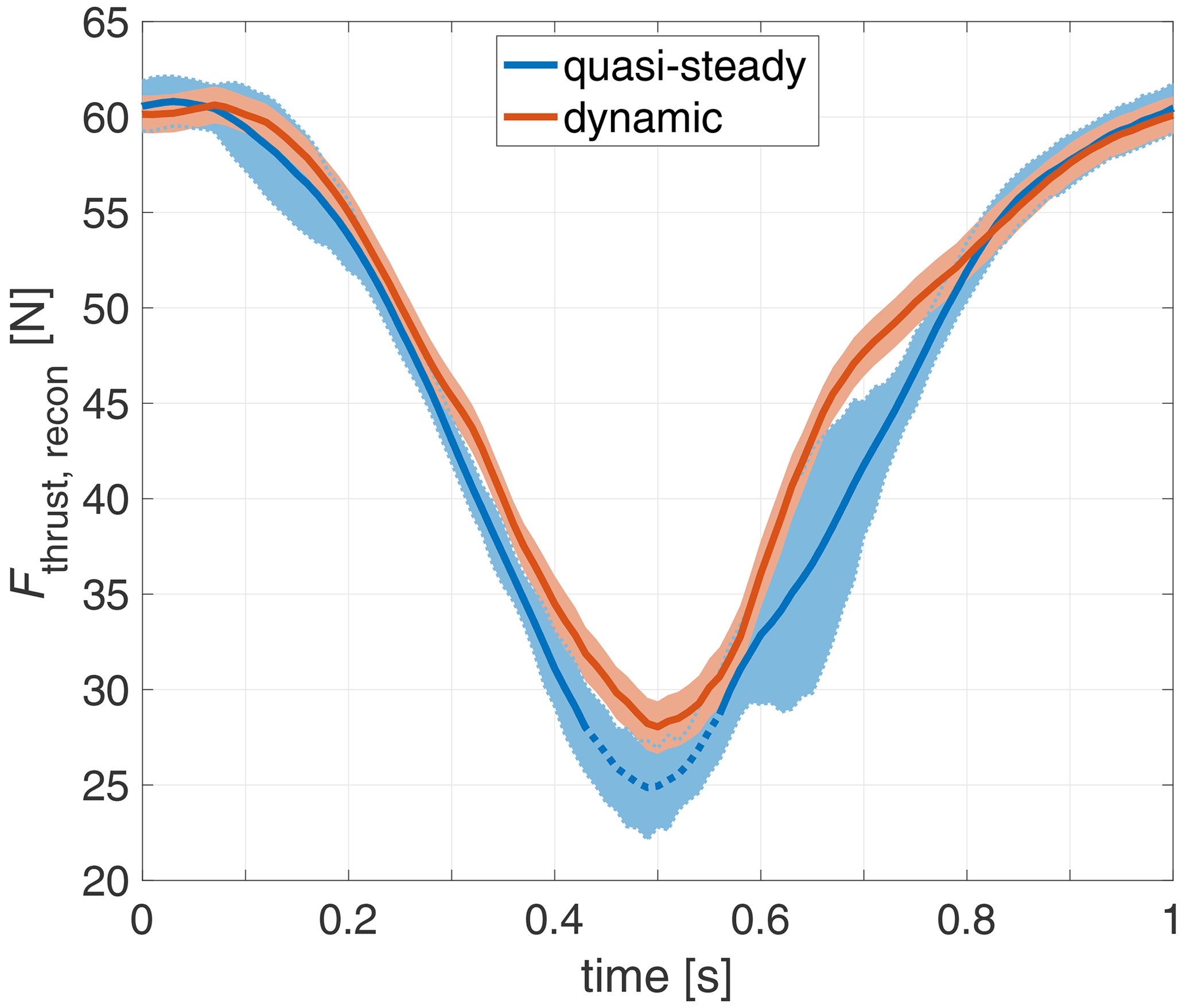
Figure 10 Thrust force reconstructed for the quasi-steady experiment and dynamic experiment from u_ax(t) and u_ta(t) for the sine wind variation. Quasi-steady u_ta(t) is used for both cases due to the low impact. Error bars are based on the quadratically added 95 % confidence intervals. Dotted values indicate the extrapolated characterisation.

3.3 Sine gust in BEM and FVWM

In Fig. 11a F_thrust(t) is shown for the sine wind field in BEM for steady operation without an engineering model and for dynamic operation with the Øye and the improved Øye dynamic inflow model (see Sect. 2.6). A clear difference can be seen between the Øye and the improved Øye model. In relation to the steady case, the Øye model leads to an increase in the load amplitude and the improved Øye model to a decrease. The difference is seen mainly at the lower tipping point.

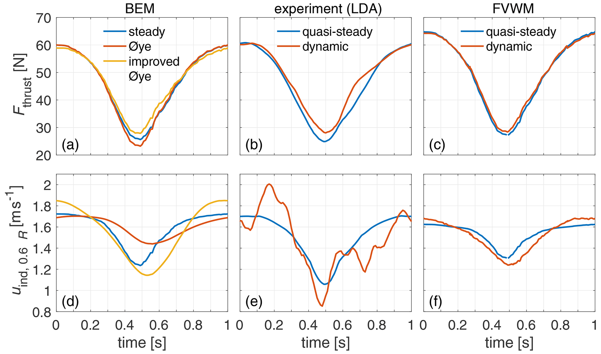
Figure 11 Steady and dynamic thrust (a) and induced velocity (d) at 0.6 R for the sine gust for BEM simulation with the original and improved Øye dynamic inflow model and correspondingly for the experiment (b, e) and the FVWM simulation (c, f). Note that (quasi-)steady cases relate to the specific experimental/simulation setup of the dynamic case.

In Fig. 11b and c, F_thrust is shown for the quasi-steady case and experimental/dynamic case for the experiment (reconstructed from the LDA measurements; reproduced from Fig. 10) and the FVWM simulation, respectively. In comparison to the steady BEM simulation, quasi-steady values are similar for the experiment and overall slightly higher (about 10 %) for the FVWM simulation. These differences are negligible here, as the analysis is based on the comparison of different cases of the same simulation environment and experiment.

For experiment and FVWM, the behaviour of the dynamic case shows a reduced load amplitude in relation to the respective quasi-steady case, with the main difference at the lower tipping point at t=0.5 s. The dynamic inflow effect modelled by the improved Øye implementation for BEM performs similar to the experiment, whereas the effect is less prominent but qualitatively similar in the FVWM simulation. In contrast to the experiment and FVWM, the original Øye model suggests the dynamic effect to increase the load amplitude.

In Fig. 11d the induced velocity u_ind(t) at the radius of 0.6 R is presented for the steady and dynamic BEM simulation – once with the original and once the improved Øye dynamic inflow model. As by design, the course of the dynamic Øye case is the filtered steady signal, reducing the amplitude of u_ind(t) compared to the steady case. In contrast, the improved Øye model leads to a higher amplitude in u_ind(t) compared to the steady case.

In Fig. 11e and f, the different quasi-steady and dynamic cases of induced velocity u_ind(t) at the radius of 0.6 R are presented for the experiment (smoothed; reproduced from Fig. 9e) and FVWM simulation, respectively. The quasi-steady cases of experiment and FVWM have a similar course as for the BEM simulation, with similar u_ind(t) values at t=0 s and some differences at the lower tipping point at t=0.5 s. As for the thrust these differences are of secondary relevance in this analysis.

The dynamic u_ind(t) of the FVWM simulation shows a very similar course to the improved Øye dynamic inflow model, compared to the respective (quasi-)steady case. This leads to an increased amplitude of the dynamic u_ind(t) compared to the quasi-steady case, with slightly higher values at the high tipping point of F_thrust(t) at t=1 s and lower values at the lower tipping point at t=0.5 s. The course of the experimental u_ind(t), compared to the respective quasi-steady case, is less explicit due to the signal noise (see Sect. 3.2.1). However, the global comparison still shows similarity to the FVWM and improved Øye, leading to an increase in the experimental signal amplitude with lower values at t=0.5 s.

In Appendix A two further comparison cases between the BEM simulations and FVWM are presented for validation. In the first comparison, the sine frequency is once doubled and once halved. In the second comparison the stochastic wind field is used as a case with different gust amplitudes. For both comparisons, the improved Øye model shows a similar performance to the here presented sine case.

4 Discussion

4.1 Turbine loads

The comparison of the steady and dynamic loads of the sine wind variation (see Fig. 7) shows a clear unsteady aerodynamic effect with a reduction in load and rotor torque amplitude for the dynamic case. The main difference is seen around the lower wind tipping point with high TSR and thus also high C_T.

The dynamic and quasi-steady loads differ for a duration of Δt=0.3 s between t=0.3 and t=0.6 s (see Fig. 7). In contrast, time constants for unsteady aerodynamic effects on the profile level, like dynamic stall and the Theodorsen effect, range from 1 to 10 ms here, estimated by the ratio of chord length to relative wind velocity. The exceeding of the stall level at the root (up to 0.25 R) at the high wind velocity tipping point further does not coincide with the phase of interest of the sine gust. As Δt is at least 30 times higher than the typical time constant for unsteady aerodynamic effects on the profile level, a relevant contribution of unsteady profile aerodynamics on the observed effect can be ruled out.

For the stochastic wind variation (see Fig. 8) the same reduction in load amplitude as for the sine gust is seen. The difference quotient in mean rotor induced velocity $\left(\frac{\mathrm{\Delta }{u}_{\mathrm{ind}}\left(t\right)}{\mathit{\tau }}\right)$ indicated this reduced response during a fast negative gust.

For the observed reduced load peak due to a positive gust, the $\frac{\mathrm{\Delta }{u}_{\mathrm{ind}}\left(t\right)}{\mathit{\tau }}$ does not give a clear indication. Similar and higher values are seen for other instances without a clear effect in M_aero(t). In contrast to other positive gust peaks, the wind tipping point at t=17 s is at a lower wind speed of 6.5 m s⁻¹, corresponding to a C_T value of 0.75 in contrast to 0.65 for the highest wind peaks and 0.83 for the lowest wind tipping points. Load variations at high C_T lead to more prominent dynamic inflow effects for the classic case of pitch steps.

4.2 Velocities in the rotor plane in experiment

The described differences between the steady and dynamic axial velocity (see Fig. 9) at the lower wind tipping point for the sine gust correspond to the effect seen in the load measurements. The lower drop of the axial velocity for the dynamic case at the lower load tipping point corresponds to a smaller reduction of the angle of attack at the respective radius and thus lower fluctuations in both local lift forces and integral load. This lower drop in axial velocity translates to a higher drop in induced velocity.

For 0.8 R, the steady case experiences a nearly constant induced velocity. Also, the dynamic case does not show strong deviations from that level. The levelled behaviour of the steady case and dynamic case at this radius is in line with current dynamic inflow modelling, which only reacts on changes in induced velocity. Amplification of the induced velocity is seen for the inner two radii for the dynamic case in comparison to the steady case for the decrease in induced velocity up to the lower tipping point.

The reconstructed steady thrust (see Fig. 10) based on these axial velocity measurements (see Sect. 2.4.2) shows a good match to the one based on the strain gauge measurement (see Fig. 7). The slight differences in the absolute levels at the tipping points (lower −1 %; upper −5 %) can be attributed to a wide range of influencing parameters including airfoil polars, tip loss model and low numbers of radii where the inductions from the experiment are available. For the direct comparison of the steady case and dynamic case, these influences cancel out as the same model is used.

For the reconstructed thrust, qualitatively the same effect as for the direct load measurement at the lower tipping point is seen, leading to a lower load amplitude for the dynamic case. The difference at the lower tipping point between the steady case and the dynamic case here is smaller, with 8 % compared to 20 % for the strain gauge measured load, each normalised by the respective quasi-steady maximum-to-minimum load difference. Considering the 95 % CI, these differences range from −2 % to 20 % for the LDA reconstructed thrust and from 10 % to 29 % for the strain gauge measured load and do show some overlap.

For the steady and dynamic axial velocity, induced velocity, and reconstructed thrust from the rotor flow, a consistent picture to the independent load measurement is given. Therefore, despite the noticeable uncertainty range of these measurements and derived flow quantities, these data give a strong indication of the dynamic inflow effect due to gusts directly in the flow.

4.3 Comparison to simulations

The Øye dynamic inflow model was experimentally validated several times, showing accurate predictions for pitch steps, e.g. for integral turbine loads in Snel and Schepers (1994), for the flow field transients in the wake by Yu et al. (2016) and for axial induction transients by Berger et al. (2020). For the investigated sine gust, an increase in dynamic load amplitude is modelled (see Fig. 11a). In contrast to the BEM simulation with the Øye dynamic inflow model, the experiment and FVWM simulation (see Fig. 11b and c) suggest a decrease in dynamic load amplitude.

The increase in dynamic load within the Øye dynamic inflow model is due to the filtering of the induced velocity. Approaching the lower load tipping point in the sine gust, the lower drop in induced velocity is equivalent to a higher drop of the dynamic axial velocity. This leads to a higher drop of the angle of attack and thus lower load. This general trend of an increase in load amplitude is therefore present for all engineering models that are based on solely filtering the induced velocities (see Schepers and Snel, 1995, for the Øye and ECN models; Yu et al., 2019, for the Yu model; and Madsen et al., 2020, for the new DTU model).

The improved Øye dynamic inflow model (see Sect. 2.6) shows the same trend of a decrease in load amplitude as the experiment and the FVWM simulation. Quantitatively the difference between steady load and dynamic load at the lower wind tipping point is at 7 %, close to the difference in thrust force based on the reconstructed thrust at 8 %. The very slightly lower dynamic load at the higher wind tipping point is seen for both the improved Øye model and the FVWM simulations.

The general trend of the induced wind velocity in the improved Øye is similar to the FVWM simulation; however, the amplification of the dynamic signal is more pronounced. In comparison, the experiment also indicates a more pronounced amplification of the induced velocity than the FVWM simulations.

This lower amplification in induced velocity of FVWM is in line with the less prominent dynamic load reduction of the FVWM compared to the experiment and the BEM simulation with the improved Øye dynamic inflow model. Together, the FVWM simulations and the experiment give a first validation of the analytically motivated improvements to the Øye dynamic inflow model.

As expected, the dynamic inflow effect due to gusts is caught by the FVWM modelling approach. The less pronounced effect on the loads is suspected to be connected to the non-perfect wake convection method, which was observed in a pitch step comparison with the same FVWM model in Berger et al. (2020). Well-tuned FVWM simulations, however, are expected to be a perfect basis for the development, tuning and validation of dynamic inflow models for gusts.

Given a wider experimental and numerical data basis, the additional term ($k_u\cdot {\mathit{\tau }}_{\mathrm{slow}}\frac{\mathrm{d}{u}_{\mathrm{0}}\left(t\right)}{\mathrm{d}t}$) for the Øye model can be further tuned. Options are to use a dedicated time constant τ_gust instead of τ_slow and to tune the parameter k_u.

4.4 Normalised comparison to Joule experiment and free field

In contrast to our findings, Snel and Schepers (1994) found no dynamic inflow effect due to gusts in their wind tunnel study with a 1.2 m diameter model wind turbine and a gust generator for approximating stepwise changes in wind velocity. Starting at an initial wind speed of 5.7 m s⁻¹ they reduced the wind velocity by 0.8 m s⁻¹ within 0.4 s, leading to a nearly linear decrease in induced velocity for the step to lower wind velocity by a maximum amount of 0.3 m s⁻¹, estimated from simulations. Divided with the respective representative dynamic inflow time constant $\mathit{\tau }=\frac{\mathrm{1}}{\mathrm{2}}\frac{R}{\stackrel{\mathrm{‾}}{u_{\mathrm{0}}}}$ (see Sect. 3.1), the maximum difference quotient of the induced velocity accounts to $\frac{\mathrm{\Delta }{u}_{\mathrm{ind}}\left(t\right)}{\mathit{\tau }}=\mathrm{0.34}$ m s⁻².

For the presented experiment, there are nearly 4 times higher values at $\frac{\mathrm{\Delta }{u}_{\mathrm{ind}}\left(t\right)}{\mathit{\tau }}=\mathrm{1.28}$ m s⁻², with Δu_ind(t)=0.4 m s⁻¹ within 0.2 s for 0.6 R at approximately t=0.4 s for the sine variation. Snel and Schepers (1994) already concluded that their change in wind velocity is not sufficiently fast to trigger clear dynamic inflow effects. This nearly 4 times higher $\frac{\mathrm{\Delta }{u}_{\mathrm{ind}}\left(t\right)}{\mathit{\tau }}$ is a plausible explanation for why the effect can be seen in the present study.

Using scaling (see Sect. 2.1) the corresponding gust events for multi MW turbines can be estimated. This would result in a sine gust with a mean wind velocity of 9.0 m s⁻¹ and amplitude of 2.5 m s⁻¹ for the NREL 5 MW reference turbine with a gust length of 50 s. This is a realistic value for a gust in the open field.

5 Conclusions

We experimentally proved the dynamic inflow effect due to gusts for wind turbines. We tested if the Øye dynamic inflow engineering model is able to predict the effect and proposed an improvement.

Firstly, experiments under reproducible gust conditions and highly resolved measurements of the longitudinal wind field proved a dynamic inflow effect due to gusts. The effect leads to damped load amplitudes and thus reduced fatigue loads. This was observed most clearly for negative gust cases at high thrust coefficients and attributed to high changes in induced velocity. For positive gusts, the effect was less pronounced and only seen for one high-thrust-coefficient configuration.

The dynamic inflow effect is also seen in the measurements of axial flow and induced velocity in the rotor plane. The effect leads to an amplification of the induced velocities. The effect is also seen in FVWM simulations for the loads and induced velocity but with slightly lower amplitudes for the induced velocity than in the experiment. Widely applied engineering models filter the induced velocities, e.g. the Øye model (Snel and Schepers, 1994) in GH Bladed and OpenFAST, the new DTU model (Madsen et al., 2020) in HAWC2, and the ECN model (Snel and Schepers, 1994) in Phatas. Exemplified by the Øye model and by analytical considerations, it was shown that such an approach cannot adequately catch the dynamic inflow phenomenon due to gusts. The filtering damps the induced velocity, thus leading to higher fatigue loads. As an initial attempt to tackle the dynamic inflow effect due to gusts, we proposed an improvement in the implementation of the Øye model, adding an additional term with a time derivative filter on the wind velocity.

Now that the effect is known further, pinpointed wind tunnel experiments are needed for the development, tuning and validation of dynamic inflow models for gusts. One focus should be to further reduce uncertainties, especially in the inflow. Furthermore, the typical operation of variable-speed-controlled wind turbine in the free field is more complex than the presented wind tunnel test. Comparisons between FVWM and BEM simulations similar to Boorsma et al. (2020) and Perez-Becker et al. (2020) but without sheared inflow can further shed light on the effect, and they can help to quantify the actual reduction in fatigue loads in realistic turbine operation for new dynamic inflow models. These new findings of dynamic inflow due to gusts are a major step to improved dynamic inflow modelling of gusts. The proposed improvement to the Øye dynamic inflow model already provides a possible first-generation dynamic inflow model to catch the general effect in BEM simulations. As this effect leads to lower fatigue loading of wind turbines, a proper and validated model opens up new design opportunities. For this aim, further coordinated research work is proposed, consisting of wind tunnel experiments and FVWM simulations.

Appendix A: Additional numerical validation cases

Two additional comparisons between the BEM model variants (steady, Øye and improved Øye model) are presented to demonstrate the applicability of the suggested approach for varying gust scenarios. The comparison is based on u_ind(t) at a radius of 0.6 R.

The first comparison is designed to qualitatively relate the reaction on a sine gust case with three different frequencies. Therefore, the time period T of one sine is doubled and halved, leading to frequencies of 0.5 and 2 Hz, respectively. The results are shown in Fig. A1a and b for the BEM variants and the FVWM simulations, respectively. The steady BEM and quasi-steady FVWM curves as well as the solid curves at T=1 s are identical to the ones on Fig. 11d and f. These curves and the differences in the (quasi-)steady values have been discussed in the context of Fig. 11. Here the focus is on the comparison of the additional curves in relation to the dynamic curve at T=1 s. For the BEM model with the Øye dynamic inflow model, T=2 s leads to a larger amplitude in u_ind(t) and T=0.5 s to a reduced amplitude, as is expected. For the improved Øye model, the change to T=2 s does not impact the minimum level at 0.5 T but just shifts it to a slightly earlier instance. For the maximum level these are slightly below the dynamic reference case. The same qualitative observations are made for the corresponding FVWM curve. For T=0.5 s, the improved Øye model and FVWM predict similar maximum values as for their respective dynamic reference case and higher minimum values closer to the minimum values of the respective (quasi-)steady curves but both with a time delay that is most obvious in the rise from the minimum to the maximum u_ind(t).

The qualitative changes for doubling and halving the sine frequency are caught by the improved Øye model as suggested by the FVWM.

In Fig. A2a and b a similar comparison is shown for the stochastic (see Fig. 8a) wind variation, providing various gust amplitudes starting from different wind velocities.

For the BEM case the original Øye dynamic inflow model gives a reduction in amplitude through the filtering approach, as is expected. The improved Øye model as well as the dynamic FVWM lead to higher amplitudes, compared to the respective (quasi-)steady cases. In general the behaviour in relation to the respective (quasi-)steady case of the improved Øye model and the FVWM are similar. However, amplitudes for the dynamic FVWM are lower than estimated by the improved Øye model, especially when the induced velocity increases. In parts these differences also reflect the difference in the respective steady signal, which shows higher amplitudes for the BEM model than for the FVWM. Also, in the comparison of a pitch step experiment in Berger et al. (2020) with this FVWM simulation setup, an offset for the fitted slow time constant, mainly for the pitch step to high load, was seen. There it was reckoned that this is related to the wake convection in the simulation model. For a further dynamic inflow gust model development based on this FVWM setup, these differences should be further investigated.

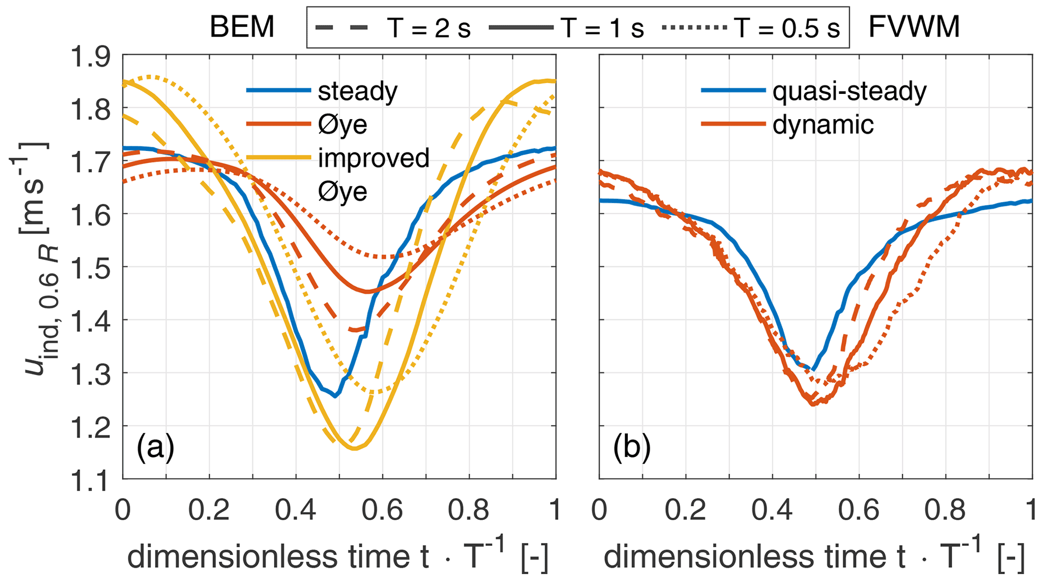
Figure A1 Steady and dynamic induced velocity at 0.6 R for the sine gust with variations in time periods for BEM simulation with the original and improved Øye dynamic inflow model (a) and FVWM simulation (b).

For a quantitative comparison, the difference between the (quasi-)steady and dynamic induced velocity at each time point is compared in a scatter plot in Fig. A3a and b, where the y axis refers to the FVWM and the x axis to the original Øye model in Fig. A3a and to the improved Øye model in Fig. A3b.

Based on the Pearson correlation coefficient (ρ_xy), the improvements in the Øye model lead from a low negative correlation to a high positive correlation, showing the good match of improved Øye and FVWM. This trend is similar for other radii. The lower y slope (0.47 x) is related to the mentioned general differences in amplitude of u_ind(t) between the models.

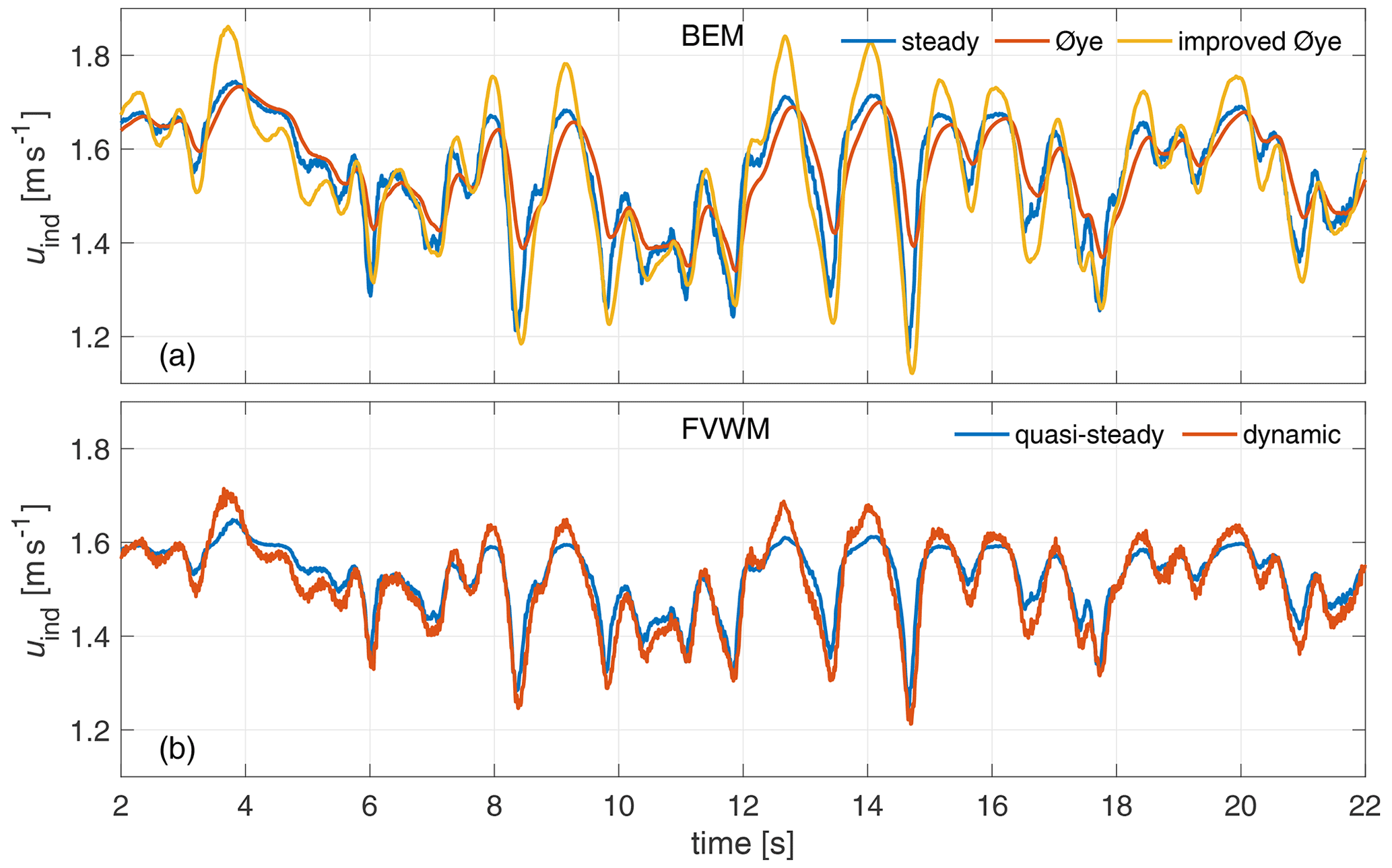
Figure A2 Steady and dynamic induced velocity at 0.6 R for the stochastic gust for BEM simulation with the original and improved Øye dynamic inflow model (a) and FVWM simulation (b).

Figure A3 Scatter plot with correlation coefficients of the differences in u_ind between the (quasi-)steady and dynamic cases of the stochastic gust at 0.6 R. Comparison of FVWM and Øye in panel (a) and FVWM and improved Øye in panel (b).

Appendix B: List of symbols

Symbol	Definition
α	angle of attack
γ	twist-and-pitch angle
θ	inflow angle
ρ	air density
ρxy	Pearson correlation coefficient
τ	time constant used for analysis
τtyp	typical single time constant for dynamic
	inflow
τfast, τslow	time constants for two-time-constant Øye
	model
Ω	angular rotor speed
a, a′	axial and tangential wake induction
c	chord length
CL, CD	lift and drag coefficients
CM, CT, Cflap	coefficients for rotor moment, thrust
	and flapwise blade root bending
	moment
D	rotor diameter
F	tip loss correction factor
FN, FT	normal and tangential force
	components
FL, FD	lift and drag force components
Fthrust	thrust force
Irot	rotational inertia of rotor and
	drivetrain
k	constant for Øye model
ku	constant for improved Øye model
Maero	aerodynamic rotor torque
Mflap	flapwise blade root bending moment
nb	number of blades
nlength, ntime	length and time scaling factors
R, r	total radius and radial position
T	time period
u0, $\stackrel{\mathrm{‾}}{u_{\mathrm{0}}}$	global (spatial mean) reference wind
	velocity (time resolved and mean)
u0,local	local reference wind velocity
uax, uta	axial and tangential velocity component
uind	induced velocity
urel	relative velocity at rotor segment