the Creative Commons Attribution 4.0 License.
the Creative Commons Attribution 4.0 License.
 | 19 Oct 2022
Offshore reanalysis wind speed assessment across the wind turbine rotor layer off the United States Pacific coast
Lindsay M. Sheridan
Raghu Krishnamurthy
Gabriel García Medina
Brian J. Gaudet
William I. Gustafson Jr.
Alicia M. Mahon
William J. Shaw
Rob K. Newsom
Mikhail Pekour
Zhaoqing Yang
The California Pacific coast is characterized by considerable wind resource and areas of dense population, propelling interest in offshore wind energy as the United States moves toward a sustainable and decarbonized energy future. Reanalysis models continue to serve the wind energy community in a multitude of ways, and the need for validation in locations where observations have been historically limited, such as offshore environments, is strong. The U.S. Department of Energy (DOE) owns two lidar buoys that collect wind speed observations across the wind turbine rotor layer along with meteorological and oceanographic data near the surface to characterize the wind resource. Lidar buoy data collected from recent deployments off the northern California coast near Humboldt County and the central California coast near Morro Bay allow for validation of commonly used reanalysis products. In this article, wind speeds from the Modern-Era Retrospective analysis for Research and Applications version 2 (MERRA-2), the Climate Forecast System version 2 (CFSv2), the North American Regional Reanalysis (NARR), the European Centre for Medium-Range Weather Forecasts Reanalysis version 5 (ERA5), and the analysis system of the Rapid Refresh (RAP) are validated at heights within the wind turbine rotor layer ranging from 50 to 100 m. The validation results offer guidance on the performance and uncertainty associated with utilizing reanalyses for offshore wind resource characterization, providing the offshore wind energy community with information on the conditions that lead to reanalysis error. At both California coast locations, the reanalyses tend to underestimate the observed rotor-level wind resource. Occasions of large reanalysis error occur in conjunction with stable atmospheric conditions, wind speeds associated with peak turbine power production (> 10 m s−1), and mischaracterization of the diurnal wind speed cycle in summer months.
- Article
(13761 KB) - Full-text XML
- BibTeX
- EndNote


This work was authored by the Pacific Northwest National Laboratory, operated for the U.S. Department of Energy (DOE) by Battelle (contract no. DE-AC05-76RL01830). The views expressed in the article do not necessarily represent the views of the DOE or the U.S. Government. The U.S. Government retains and the publisher, by accepting the article for publication, acknowledges that the U.S. Government retains a nonexclusive, paid-up, irrevocable, worldwide license to publish or reproduce the published form of this work, or allow others to do so, for U.S. Government purposes.
As countries around the globe endeavor to decarbonize their economies, offshore wind is gaining momentum to help achieve targeted emission goals. In 2020, the cumulative global offshore wind capacity stood at 33 GW, with Europe leading the world in offshore deployment, followed by China (Musial et al., 2021). In North America, offshore wind is still nascent and only recently became an important resource of focus. This is primarily due to improvements in rates of return, technological efficiencies, transmission, and confidence stemming from European success (Dong et al., 2021). In 2020, the US offshore wind project development and operational pipeline stood at a potential generating capacity of 35 GW (Musial et al., 2021). While much of the offshore wind project development and operational pipeline activity is currently concentrated along the Atlantic coast, enthusiasm for harvesting the wind resource along the Pacific coast is building (Wang et al., 2019).
Stemming from their essential role in the onshore wind market, reanalysis models are supporting global offshore wind development and operation in a multitude of ways. These decades-long meteorological and climate data assimilation products are utilized by the offshore wind community to produce site assessments (Nehzad et al., 2021), simulate long-term power generation (Hayes et al., 2021), and provide estimates of the levelized cost of energy (de Assis Tavares et al., 2022). Given their crucial position in the offshore wind development and operation cycles, validation of reanalyses is imperative to instill and maintain investor confidence and to set appropriate expectations of power production for load-balancing operatives.
Validations of reanalysis-based wind resource assessments in an offshore wind energy context have been limited in the past due to a scarcity of observations, particularly across typical turbine rotor layer heights, which range from approximately 25 to 200 m for current turbine technology and are projected to range from approximately 25 to 275 m for future turbine technology (Musial et al., 2019). Recent advancements in floating lidar technology, however, have propelled opportunities to enhance understanding of the marine boundary layer while providing the necessary rotor-level height observations for comparisons with commonly employed reanalyses. Using a lidar system off the coast of India, Jani et al. (2019) noted that the European Centre for Medium-Range Weather Forecasts (ECMWF) ERA-Interim reanalysis underestimates observed 80 and 100 m above sea level (a.s.l.) wind speeds by 1.2 m s−1. Comparing the ECMWF Reanalysis v5 (ERA5) with observations from a meteorological tower aboard an oil platform, Fernandes et al. (2021) found zero bias, a root-mean-square error (RMSE) of 2.3 m s−1, and a Pearson correlation coefficient of 0.8 at 100 off the coast of Brazil. In the United States, Pronk et al. (2022) utilized a floating lidar off the coast of New Jersey and noted that ERA5 produces rotor-level biases near −1 m s−1, centered root-mean-square errors (CRMSEs) around 1.5 m s−1, and squared correlation coefficients near 0.9 at heights ranging from 58 to 198
The U.S. Department of Energy (DOE) lidar-mounted buoys deployed for a year off the coasts of New Jersey and Virginia showed consistent reanalysis and model underestimation of wind speed at 90 (Sheridan et al., 2020). For these Atlantic locations, ERA5 and Rapid Refresh (RAP) showed high correlation with the 90 m wind speed observations (Pearson correlation coefficient of ∼ 0.9) and a RMSE of ∼ 1.9 m s−1. Significant reanalysis underestimation and reduced correlation was noted during the summer at the New Jersey and Virginia buoy locations (Sheridan et al., 2020). Atlantic meteorological and synoptic conditions such as sea breezes, tropical storms, and coastal upwelling and downwelling conditions were identified as some of the typical causes for reanalysis-based wind speed errors (Sheridan et al., 2020).
In this article, multi-season measurements from two buoy deployments off the coast of California are analyzed. The wind resource along the Pacific coast of California is influenced by diverse physical characteristics, such as low-level jets (Parish, 2000), coastally trapped wind reversals (Bond et al., 1996), atmospheric hydraulic jumps (Juliano et al., 2017), Santa Ana winds (Rolinski et al., 2019), and California expansion fans (Parish et al., 2016). The marine boundary layer along the western coast is heavily influenced by the coastline. The points and capes near the two lidar buoys (Cape Mendocino near Humboldt and Point Conception near Morro Bay) significantly impact the marine boundary layer. These features influence the wind and temperature fields, creating stronger gradients along the coast. These conditions can also result in horizonal ducting, which influences microwave transmission within the region (Haus et al., 2022). Fog and low-level stratus are also frequently observed along the California coast (Koracin et al., 2014). Fog formation within the region is primarily due to advection of moist air over cold upwelled waters. Fog is observed mostly during summer months. Clouds also influence satellite retrievals of various sea state parameters (such as sea surface temperature), which are typically used in reanalysis models. A lack of long-term offshore boundary layer observations for data assimilation into reanalysis models results in larger errors in offshore conditions. In general, complex conditions are observed along the coast of California, and modeling of the wind resource remains a continuous challenge to the research community. The sources of error in reanalysis models could vary and compound due to different model grid resolution, vertical extrapolation errors due to Monin–Obukhov similarity theory, an appropriate choice of climate models in various reanalysis, planetary boundary layer schemes chosen within each model, local conditions, and different data assimilation data types in each reanalysis.
Analysis of the wind observations collected during the California deployments of the DOE lidar buoys is provided in Sect. 2, along with descriptions of the models and satellite observations used in this study. Section 2 concludes with a discussion of the error metrics selected to validate each reanalysis and analysis model. Section 3 examines the overall performances of the models during the California deployment period and continues with a breakdown of performance according to a variety of temporal and physical characteristics, such as trends according to seasonal and diurnal cycles, atmospheric stability, wind shear, wind reversals, and case studies on major atmospheric phenomena observed during the buoy deployments. Finally, Sect. 4 summarizes the results to provide an understanding of the capabilities and limitations associated with reanalysis-based wind resource assessment in California coastal areas of offshore wind development interest.
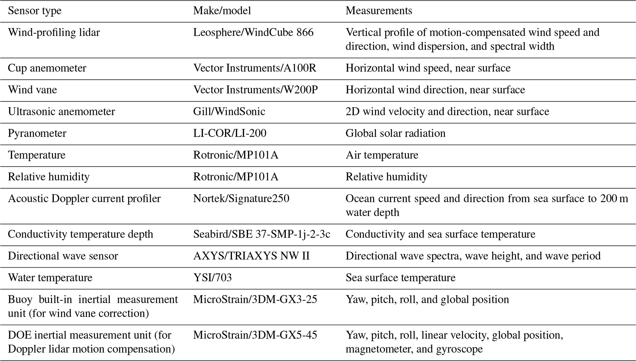
The DOE owns two AXYS WindSentinel™ buoys mounted with Leosphere WindCube v2 lidar systems and surface meteorological and oceanographic (metocean) instruments (Severy et al., 2021). Prior to their deployment off the California coast, the DOE lidar buoys underwent extensive validation administered by Ocean Tech Services and Det Norske Veritas (DNV) at the Martha's Vineyard Coastal Observatory operated by Woods Hole Oceanographic Institute in the spring of 2020. The validation was performed against an International Electrotechnical Commission-certified (IEC) reference lidar approximately 250 m away on an offshore platform (Air–Sea Interaction Tower). The comparison yielded wind speed coefficients of determination (R2) greater than 0.98 and wind direction R2 values greater than 0.97 at heights up to 200 (Gorton and Shaw, 2020).
In the fall of 2020, the buoys were deployed off the northern and central coasts of California (Fig. 1). The central buoy was deployed in 1100 m of water approximately 40 km from the shore near Morro Bay (35.7107∘ N, 121.8581∘ W). The Morro Bay buoy was deployed from 29 September 2020 to 19 October 2021. The northern buoy was deployed in 625 m of water approximately 40 km off the coast of Humboldt County (40.97∘ N, 124.5907∘ W). The Humboldt buoy deployment period began on 1 October 2020 and is estimated to conclude in May 2022. A large wave event in December 2020 disabled the buoy power supply, which resulted in a significant gap in the data availability during the first year of deployment (Fig. 2d). In this article, the period of study for both buoys is 1 October 2020 to 27 December 2020 and 25 May 2021 to 30 September 2021. Additionally, the full seasonal cycle of 1 October 2020 to 30 September 2021 is analyzed for Morro Bay.

Figure 1Locations of the DOE buoys and nearby National Data Buoy Center buoys 46022 and 46028. The purple-shaded regions around the buoys show Bureau of Ocean Energy Management wind energy areas as of 12 January 2022. GEBCO: General Bathymetric Chart of the Oceans. NGDC: National Geophysical Data Center.
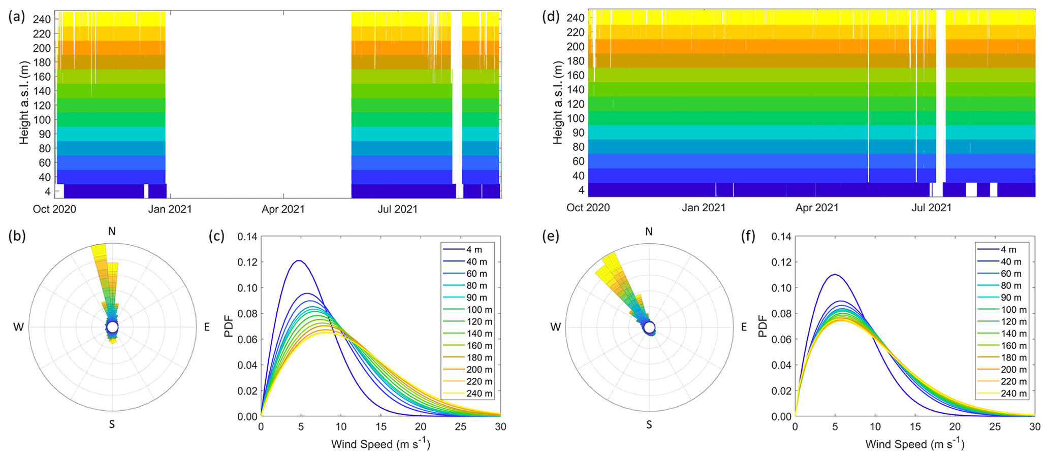
Figure 2Observational coverage of the (a) Humboldt and (d) Morro Bay deployments, observed 100 m wind roses from the (b) Humboldt and (e) Morro Bay deployments, and Weibull fits to wind speed observations from the (c) Humboldt and (f) Morro Bay deployments. PDF: probability density function.
2.1 Buoy instrumentation and observations
During the California deployments, the instruments were identical on both buoys as listed in Table 1. The buoys collect metocean observations including wind speed and direction from the surface up to 250 and current profiles down to 200 m below the sea surface. A complete description of the instrumentation aboard the buoys is provided in Severy et al. (2021).
The winds at the buoy deployment locations predominantly follow the California coastline, northerly at Humboldt (Fig. 2b) and northwesterly at Morro Bay (Fig. 2e). The average wind speed at 100 is 9.0 m s−1 over the Humboldt deployment, 7.9 m s−1 at Morro Bay during the overlapping Humboldt period, and 8.6 m s−1 over the full Morro Bay deployment. Applying the reference 6 MW power curve of Musial et al. (2019), the 100 m wind speeds translate to deployment-wide gross capacity factors (the ratio of simulated deployment-wide energy in kilowatt hours with the product of turbine rated capacity and the number of hours in the deployment) of 55.5 % at Humboldt, 45.7 % at Morro Bay during the overlapping Humboldt period, and 51.0 % at Morro Bay during the full seasonal cycle (without taking into effect any operational losses, such as wakes and turbine availability).
Table 2Characteristics of the models that produce rotor-level wind speed estimates.

a 1979–2010 is available as CFSR. b The data have been converted from the native reduced Gaussian grid to a regular latitude–longitude grid at 0.5∘ (Saha et al., 2011). c The data have been converted from the native reduced Gaussian grid to a regular latitude–longitude grid at 0.25∘ (Hersbach et al., 2020).
2.2 Reanalysis and analysis models
Five reanalysis and weather forecast analysis models are investigated for their performance in representing the offshore wind resource at the lidar buoy locations off the California coast. MERRA-2 (Modern-Era Retrospective analysis for Research and Applications version 2) from the National Aeronautics and Space Administration (NASA) Global Modeling and Assimilation Office (GMAO) is a global reanalysis that covers the modern satellite era (Gelaro et al., 2017). The Climate Forecast System version 2 (CFSv2) from the National Oceanic and Atmospheric Administration (NOAA) National Centers for Environmental Prediction (NCEP) is a global operational forecast model that runs four times daily and is extended temporally by its reanalysis component, the Climate Forecast System Reanalysis (CFSR) (Saha et al., 2011, 2014). NARR (North American Regional Reanalysis) from NOAA NCEP is a reanalysis with spatial coverage over North America and temporal coverage over the modern satellite era (Mesinger et al., 2006). ERA5 from ECMWF is a global reanalysis with the longest temporal coverage of the five models assessed in this work, extending from 1950 (Hersbach et al., 2020). RAP is an operational forecast model covering North America with a temporal extent covering the last 10 years (Benjamin et al., 2016). The analysis system of RAP is considered in this study. Since this study uses a combination of analysis and reanalysis data, we will refer to these collectively as model data henceforth for simplification. Spatial and temporal characteristics of the five models are provided in Table 2.
Several of the models provide wind data at turbine hub heights in support of the wind energy industry (Ramon et al., 2019). MERRA-2 outputs wind data at 50 m, which are interpolated from the lowest native level using the Helfand and Schubert scheme (Helfand and Schubert, 1995). The Helfand and Schubert scheme uses modified Monin–Obukhov similarity theory (MOST) with roughness length parameterized as in Large and Pond (1981). RAP outputs wind data at 80 m, which are determined by interpolation between the surrounding prognostic model levels (Benjamin et al., 2020). ERA5 outputs wind data at 100 m, which are derived using MOST with open-terrain roughness (Ramon et al., 2019). Additionally, three models (RAP, CFSv2, and NARR) output wind data at the lowest 0–30 mbar layer above sea level. This variable represents the average wind speed over the layer from the surface to the height at which the air pressure is equal to the surface pressure minus 30 mbar. This output layer is frequently used by the industry to be representative of hub height winds. Therefore, a thorough evaluation of this output with lidar measurements at various altitudes would help the wind industry tailor their wind resource expectations from the models.
2.3 Near-surface wind data
In order to provide a more comprehensive analysis of the wind off the California coast, two additional data sources providing near-surface wind speed data are considered. The NOAA National Data Buoy Center (NDBC) maintains historical and current observational data from a network of buoys across US waterways (NDBC, 2021). Two NDBC buoys are located near the DOE lidar buoy deployment locations at Humboldt and Morro Bay, each of which provide wind speed information at 4 , which is consistent with the anemometer height aboard the DOE buoys. NDBC buoy 46022 is located at 40.748∘ N, 124.527∘ W, approximately 25 km south-southeast of the DOE Humboldt buoy, and provides wind speed observations with a data recovery of 91 % over the period 1 October 2020 through 30 September 2021. NDBC buoy 46028 is located at 35.77∘ N, 121.903∘ W, approximately 8 km northwest of the DOE Morro Bay buoy and provides wind speed observations with a data recovery rate of 96 % over the period 1 October 2020 through 30 September 2021.
Ribal and Young (2019) provide a 33-year collection of satellite-derived 10 m wind speeds from 14 altimeters with global coverage. Satellite near-surface wind data from CryoSat-2, Jason-3, SARAL (Satellite with ARgos and ALtiKa, Ka-band altimeter), Sentinel-3A, and Sentinel-3B with a quality control flag of 1, indicating good data, are utilized in this study, and the uncalibrated version is chosen in order to align with the data that are assimilated into the reanalyses. The satellite data offer sporadic near-surface wind speed measurements because satellites follow multi-day repeat tracks. The temporal resolution along the tracks is high, approximately 1 Hz (Ribal and Young, 2019). At total of 627 and 203 satellite data points are collected between October 2020 and September 2021 within a 30 km radius of the Humboldt and Morro Bay buoys, respectively, at times spanning the diurnal cycle, though no individual days provide complete representation of the diurnal cycle. Seasonally, satellite data representation is balanced across all months between October 2020 and September 2021, except July, August, and September, when little to no satellite data are available due to the possible presence of low-level clouds or fog.
2.4 Atmospheric stability data
Atmospheric stability is a major influence on the shape of the vertical wind speed profile and therefore on the amount of power that can be derived from a wind turbine (Wharton and Lundquist, 2012). To assess the impact of atmospheric stability on model wind speed performance, the Obukhov length L is estimated using the Tropical Ocean-Global Atmosphere Coupled Ocean–Atmosphere Response Experiment (TOGA COARE) version 3.6 algorithm using the near-surface DOE buoy metocean observations at Humboldt and Morro Bay (Fairall et al., 1996; Edson et al., 2013). Typically, L is defined as
where Tv is the virtual temperature, u∗ is the friction velocity, k is the von Kármán constant, g is gravitational acceleration, and is the kinematic virtual temperature flux. In COARE version 3.6, the Obukhov length can be expressed as an effective function of the bulk Richardson number (Grachev and Fairall, 1997). The bulk Richardson number is defined purely using standard meteorological and oceanic mean observations and is given by
where Δθv is the virtual potential temperature difference between the water surface and atmosphere, T is the air temperature, U is the magnitude of the mean wind vector, and z is the height of measurement.
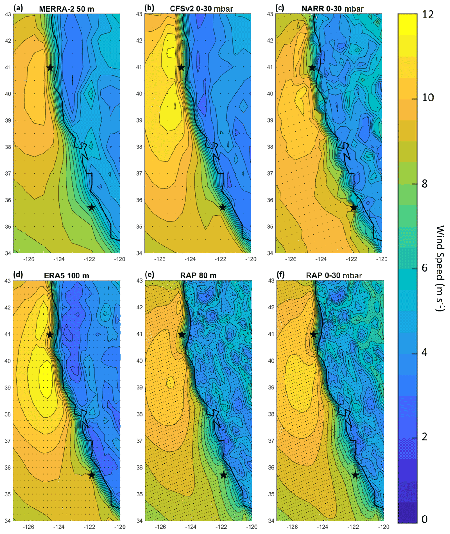
Figure 3Average wind speed over the period 1 October 2020 through 30 September 2021 from (a) MERRA-2 at 50 , (b) CFSv2 over the lowest 0–30 mbar layer above sea level, (c) NARR over the lowest 0–30 mbar layer above sea level, (d) ERA5 at 100 m, (e) RAP at 80 m, and (f) RAP over the lowest 0–30 mbar layer above sea level. Buoy deployment locations are indicated with stars. Model grid points are indicated with dots.
2.5 Methodology
Given the location of both DOE buoys within or near the dense wind speed contours along the coastline (Fig. 3), selecting the nearest-neighbor model grid point does not provide a representative baseline for comparison between simulated and observed wind speeds. Therefore, distance-weighted interpolation using the surrounding model grid points is applied to approximate the simulated wind speed at the buoy locations. Vertically, models with single-level output heights that align with the lidar output heights, i.e., RAP at 80 and ERA5 at 100 , are directly compared with the observations at that height. For MERRA-2 at 50 m, a height that does not align with the lidar output heights, the observations at 40 and 60 m are linearly interpolated to 50 m to provide comparison at that height. For the three models that output wind speed data over the lowest 0–30 mbar layer above sea level (CFSv2, NARR, and RAP), comparisons are performed using the lidar buoy observations at all output heights between 80 and 120 m to determine which hub height(s) the layer best represents.
Temporally, comparisons between observed and model wind speeds are performed according to the resolution of the model, namely on a 3-hourly basis for NARR and a 1-hourly basis for MERRA-2, CFSv2, ERA5, and RAP. The processed lidar buoy observations are averaged over a 10 min period, with the timestamp reflecting the start of the averaging period. The lidar buoy observations at the top of each hour are selected for comparison with the models. The NDBC buoy observations are averaged over a 10 min period, with the timestamp reflecting the end of the averaging period. The NDBC buoy observations at 10 min after the hour are therefore selected to align with the averaging period of the lidar buoy observations. Given the temporal coarseness of the satellite winds, wind data from this collection are down-selected within a 30 km radius of the buoys and considered for their average and distribution characteristics.
In order to assess the accuracy of model representation of observed wind speeds, the wind speed validation employs three error metrics: wind speed bias, centered root-mean-square error (CRMSE), and correlation coefficient. The wind speed bias, i.e., the average difference over a time series of length N between the modeled (vmod) and observed (vobs) wind speeds, conveys whether a model tends to overestimate (positive bias), underestimate (negative bias), or accurately represent (zero bias) the observed wind resource:
The CRMSE describes the variation in error between modeled and observed wind speeds, with larger values corresponding to larger error:
Finally, the Pearson correlation coefficient describes the degree to which the modeled and observed wind speeds are linearly related, with values close to one indicating a high degree of correlation:
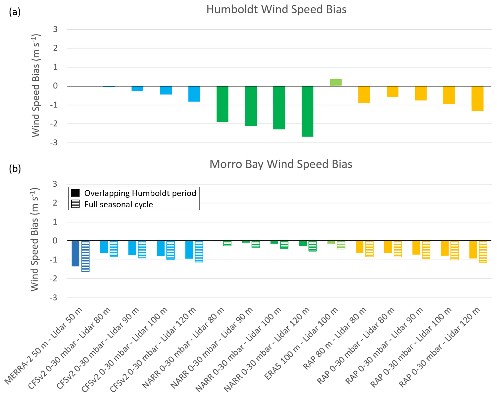
Figure 4Wind speed biases during the (a) Humboldt and (b) Morro Bay deployments. The Morro Bay biases are provided for the overlapping Humboldt recovery periods of 1 October 2020–27 December 2020 and 25 May 2021–30 September 2021 (solid) and for the entire Morro Bay collection period that covers a full seasonal cycle (striped).
3.1 Model wind speed performance over the California deployments
At the Humboldt and Morro Bay sites, the models tend to underestimate the observed rotor-level wind speeds (Fig. 4). Beginning with the direct model level to lidar level comparisons at Morro Bay, MERRA-2, the coarsest of the models, strongly underestimates the average observed wind speed at 50 with a bias of −1.6 m s−1 over the full deployment period and 1.3 m s−1 over the overlapping Humboldt data recovery periods of 1 October 2020–27 December 2020 and 25 May 2021–30 September 2021. Meanwhile at Humboldt, MERRA-2 exhibits almost no bias at 50 m. ERA5 overestimates the observed 100 m wind speed at Humboldt by 0.4 m s−1 and underestimates the observed 100 m wind speed at Morro Bay with biases of −0.1 and −0.4 m s−1 for the overlapping Humboldt periods and full seasonal cycle, respectively. At 80 , RAP underestimates with similar biases at each deployment site, −0.9, −0.6, and −0.8 m s−1 at Humboldt, Morro Bay (overlapping Humboldt period), and Morro Bay (full seasonal cycle), respectively.
Using the lowest 0–30 mbar layer above sea level to approximate the hub height, wind resource produces negative biases at both lidar buoy sites regardless of the observed hub height selected for comparison (Fig. 4). At each site and for each model (CFSv2, NARR, and RAP), the average simulated wind speed produced using the lowest 0–30 mbar layer is closest to the average observed wind speed at 80 m. Comparable in horizontal resolution to MERRA-2, CFSv2 similarly produces an 80 m wind speed bias near zero at Humboldt and biases of −0.7 and −0.8 m s−1 at Morro Bay for the overlapping Humboldt period and the full seasonal cycle, respectively. NARR exhibits zero bias at Morro Bay during the overlapping Humboldt period, underestimates the observed 80 m wind speed by 0.3 m s−1 at Morro Bay over the full seasonal cycle, and drastically underestimates the observed 80 m wind speed by 1.9 m s−1 at Humboldt. Using the lowest 0–30 mbar layer above sea level, RAP produces 80 m wind speed biases of −0.8, −0.6, and −0.6 m s−1 at Morro Bay (full seasonal cycle), Morro Bay (overlapping Humboldt period), and Humboldt, respectively, the last of which is smaller than the bias produced using the direct RAP 80 m output level at Humboldt.
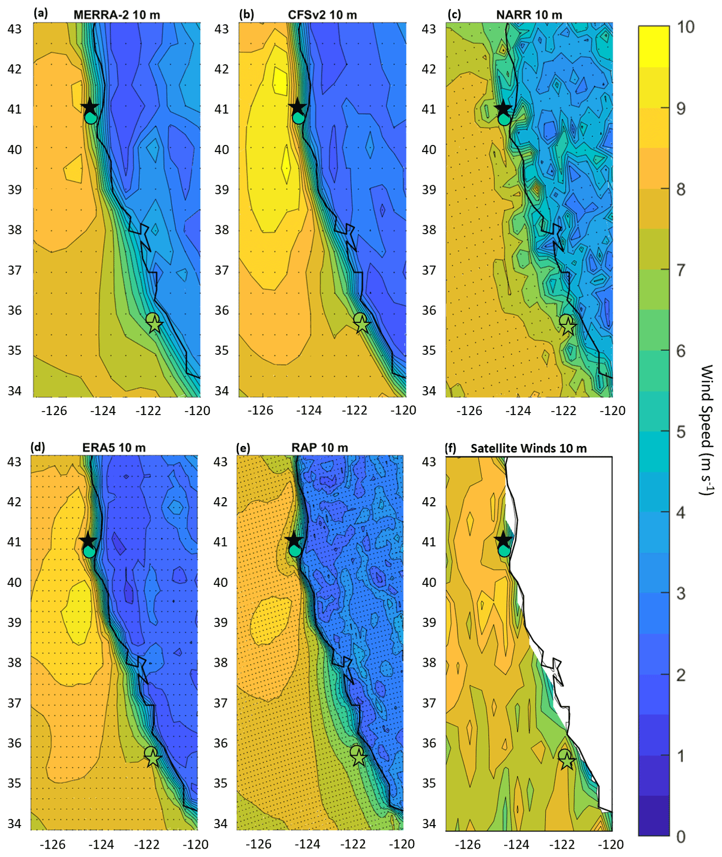
Figure 5Average wind speed over the period 1 October 2020 through 30 September 2021 from (a) MERRA-2 at 10 , (b) CFSv2 at 10 , (c) NARR at 10 , (d) ERA5 at 10 , (e) RAP at 10 , and (f) the satellite winds at 10 . Model grid points are indicated with dots. DOE buoy locations are indicated with stars, and Morro Bay is colored to reflect the average 4 wind speed over the period 1 October 2020 through 30 September 2021 (6.6 m s−1). NDBC buoy locations are indicated with circles and are colored to reflect the average 4 wind speed over the period 1 October 2020 through 30 September 2021 (5.8 m s−1 at the northern Humboldt location and 6.7 m s−1 at the central Morro Bay location).
An examination of modeled and observed wind speed behavior near the surface, the level at which buoy observations and satellite winds are assimilated into reanalyses, is performed. With the exception of NARR, the models and the satellite winds at 10 m capture the enhanced wind speeds within the expansion fan caused by the bend in the California coastline at 40∘ N (Fig. 5). MERRA-2, CFSv2, and the satellite winds show two locations of wind speed maxima, to the north and south of the Humboldt buoy, while ERA5 and RAP concentrate the fastest wind speeds to the south of the Humboldt buoy.
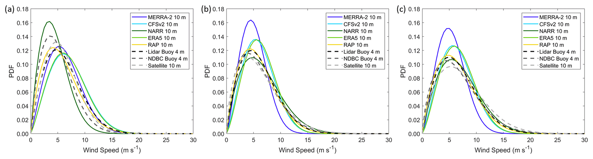
Figure 6Weibull fits to near-surface observed, modeled, and satellite winds at (a) Humboldt, (b) Morro Bay during the overlapping Humboldt period, and (c) Morro Bay during the full seasonal cycle.
The supercritical flow that is developed south of Humboldt at Cape Mendocino results in increasing wind speeds south of the cape creating an expansion fan (Dorman and Winant, 1995; Haack and Burk, 2001). The satellite winds and models show the DOE Humboldt buoy and neighboring NDBC buoy 46022 located within a swath of rapid wind speed deceleration between the expansion fan zone and the California coast (Fig. 5). Weibull fits to the near-surface wind speeds at Humboldt reveal consistent distributions for the buoy observations; satellite winds; and MERRA-2, CFSv2, ERA5, and RAP wind speeds, with the buoy observations yielding slightly slower distributions reflective of the lower measurement height of 4 m (Fig. 6a). NARR at 10 m shows substantially slower wind speeds than the observations, satellite winds, and other models at Humboldt, consistent with the trends in rotor layer wind speed bias (Fig. 4a).
The satellite winds, CFSv2, and ERA5 show a swath of 10 m wind speed between 7.5 and 8 m s−1 extending toward the DOE Morro Bay buoy and neighboring NDBC buoy 46028, at approximately 35.5∘ N, 122∘ W (Fig. 5). MERRA-2, NARR, and RAP place 10 m wind speeds in this range further from shore and therefore further from the observational buoys. The MERRA-2 wind speed deceleration zone near Morro Bay is particularly large in geographic extent. Weibull fits to the near-surface wind speeds at Morro Bay show similar behavior between CFSv2 and ERA5, with 10 m distributions peaking around 6 m s−1 (Fig. 6b and c). The NARR and RAP 10 m distributions are similar to the DOE and NDBC buoy distributions at 4 m. MERRA-2 at 10 m shows drastically slower wind speeds than the observations, satellite winds, and other models at Morro Bay, a finding that aligns with the trends in rotor-level wind speed bias noted in Fig. 4b.
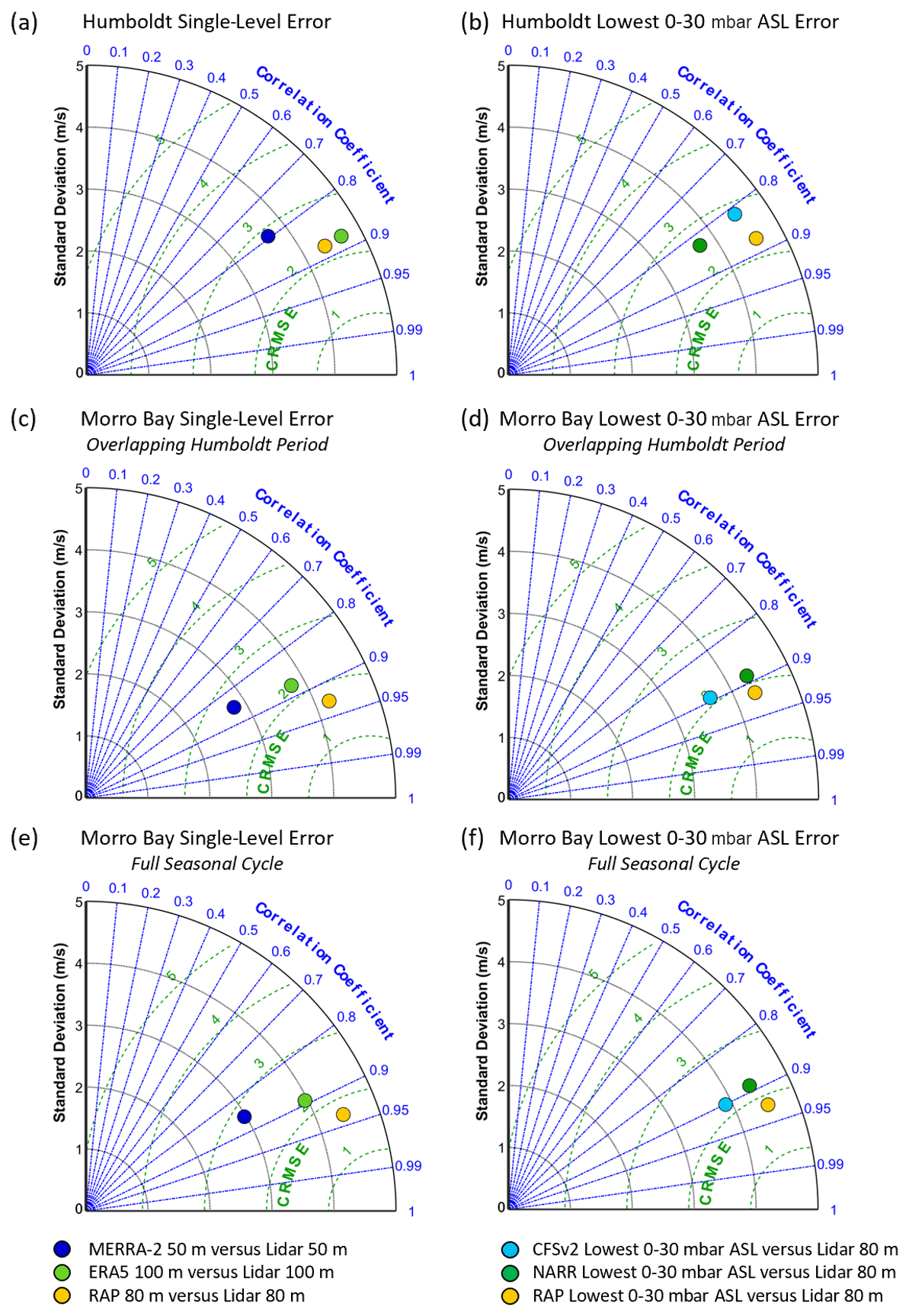
Figure 7Taylor diagrams of single-level model error at (a) Humboldt and (c) Morro Bay and error using the lowest 0–30 mbar layer above sea level to simulate hub height at (b) Humboldt and (d) Morro Bay.
For the performance metrics of CRMSE and correlation, RAP is the best performing model at both sites, regardless of whether the direct 80 m output level or the lowest 0–30 mbar layer above sea level is employed (Fig. 7). The high spatial resolution of RAP is a likely factor in the model success, providing ability to represent features and phenomena that the coarser models miss, as is explored in upcoming sections. It is also possible that the relatively rapid analysis cycle of RAP (hourly) versus some of the reanalyses may be a factor. Beginning with the direct comparisons of model level to lidar level, RAP, ERA5, and MERRA-2 produce CRMSEs of 2.3, 2.4, and 2.7 m s−1, respectively, and correlations of 0.88, 0.88, and 0.79, respectively, at Humboldt. RAP, ERA5, and MERRA-2 produce CRMSEs of 1.7, 2.3, and 2.4 m s−1, respectively, and correlations of 0.93, 0.88, and 0.85, respectively, at Morro Bay during the overlapping Humboldt data recovery periods of 1 October 2020–27 December 2020 and 25 May 2021–30 September 2021. Finally, RAP, ERA5, and MERRA-2 produce CRMSEs of 1.7, 2.3, and 2.6 m s−1, respectively, and correlations of 0.94, 0.89, and 0.86, respectively, at Morro Bay during the full seasonal cycle of 1 October 2020–30 September 2021.
Simulating wind speeds at 80 m using the RAP, CFSv2, and NARR lowest 0–30 mbar layer above sea level produces CRMSEs of 2.3, 2.8, and 2.6 m s−1, respectively, and correlations of 0.88, 0.82, and 0.83, respectively, at Humboldt (Fig. 7). During the overlapping Humboldt period at Morro Bay, RAP, CFSv2, and NARR at the lowest 0–30 mbar layer above sea level produce CRMSEs of 1.8, 2.1, and 2.1 m s−1, respectively, and correlations of 0.92, 0.89, and 0.89, respectively, compared to observed 80 m wind speeds. At Morro Bay during the full seasonal cycle, RAP, CFSv2, and NARR at the lowest 0–30 mbar layer above sea level produce CRMSEs of 1.8, 2.2, and 2.3 m s−1, respectively, and correlations of 0.93, 0.90, and 0.89, respectively, compared to observed 80 m wind speeds. The model-based rotor-level correlations during the Humboldt and Morro Bay deployments are similar to or exceed the near-surface correlations determined by Wang et al. (2019) comparing NDBC buoy observations along the California coast with NARR and MERRA (version 1).
While comparing the lowest 0–30 mbar layer above sea level with different observational heights (80–120 m) produces noticeable variability in the resultant biases (Fig. 4), with the lowest bias occurring when comparing with the observations at 80 m, correlation and CRMSE do not show a trend with varying observational height. Standard deviations in the CRMSEs produced when comparing the lowest 0–30 mbar layer above sea level with observations at 80, 90, 100, and 120 m range from 0.04 (RAP at Humboldt, best case) to 0.1 m s−1 (NARR at Humboldt, worst case). Standard deviations in the correlations produced when comparing the lowest 0–30 mbar layer above sea level with observations at 80, 90, 100, and 120 m range from 0.06 % (RAP at Morro Bay, best case) to 0.2 % (NARR at Humboldt, worst case).
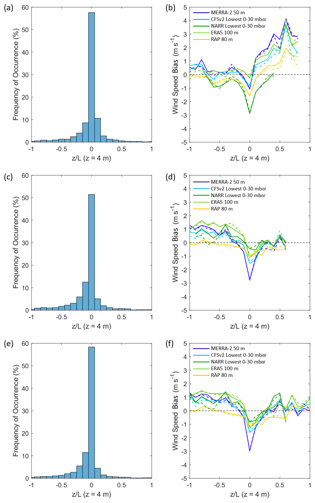
Figure 8Distributions of stability parameter during (a) the Humboldt deployment, (c) the Morro Bay deployment during the Humboldt overlapping period, and (e) the Morro Bay deployment during the full seasonal cycle. Average (solid) and median (dashed) rotor-level wind speed bias according to during (b) the Humboldt deployment, (d) the Morro Bay deployment during the Humboldt overlapping period, and (f) the Morro Bay deployment during the full seasonal cycle, calculated over intervals of length 0.1. Intervals with less than 10 samples are excluded.
3.2 Model performance according to atmospheric stability
The COARE model in conjunction with the near-surface measurements from the DOE lidar buoys enables an examination of model performance according to atmospheric stability. The dimensionless ratio (z = 4 m) is concentrated around zero for both the Humboldt and Morro Bay deployments (Fig. 8a, c, and e), indicating a predominance of near-neutral atmospheric conditions. Outside of neutral conditions, Morro Bay conditions tend toward unstable ( < 0) during the full seasonal cycle and the overlapping Humboldt period, while the Humboldt conditions are more evenly distributed among unstable and stable ( > 0). A contributing factor for the difference in stability between the two locations is the air–sea temperature differential. At the northern Humboldt location, the average air temperature and sea surface temperature during the deployment are both 12.0 ∘C. Further south at Morro Bay, the average air and sea surface temperatures increase as expected, however not equally. The average air and sea surface temperatures at Morro Bay during the overlapping Humboldt deployment period are 13.9 and 14.6 ∘C, respectively. The trend of cooler air relative to warmer ocean results in more frequent unstable conditions.
For both the Humboldt and Morro Bay deployments, the models show the strongest underestimation of the observed rotor-level wind speeds when atmospheric conditions near the surface are near neutral ( 0). At Humboldt, MERRA-2, CFSv2, NARR, ERA5, and RAP produce rotor-level wind speed biases of −1.1, −0.8, −2.9, −0.3, and −1.6 m s−1, respectively, when −0.05 < 0.05 (Fig. 9b). At Morro Bay during the overlapping Humboldt period, MERRA-2, CFSv2, NARR, ERA5, and RAP produce rotor-level wind speed biases of −2.8, −1.5, −0.5, −1.1, and −1.1 m s−1, respectively (Fig. 8d). During the Morro Bay full seasonal cycle, MERRA-2, CFSv2, NARR, ERA5, and RAP produce rotor-level wind speed biases of −3.0, −1.6, −0.8, −1.3, and −1.3 m s−1, respectively (Fig. 8f).
At Humboldt, the biases in the unstable regime are confined between ± 1 m s−1, while in the stable regime the biases indicate strong model overestimation of the observed wind speeds, with biases in excess of 2 m s−1 for MERRA-2, CFSv2, and ERA5 (Fig. 8b). At Morro Bay, the trend is reversed, as the models most strongly overestimate the observed rotor-level wind speeds in the unstable regime, with all models except RAP exhibiting biases near 1 m s−1 (Fig. 8d and f). As with Humboldt in unstable conditions, the biases at Morro Bay during stable conditions tend to be confined between ± 1 m s−1 (Fig. 8d and f). The accuracy of using MOST for wind profile extrapolation varies according to atmospheric stability, with larger errors typically occurring during stable atmospheric conditions (Optis et al., 2015). Since models use MOST to extrapolate within the lowest grid levels, the propagation of error in the models is dependent on the accuracy of the chosen MOST application, such as Businger et al. (1971) and Dyer (1974), Beljaars and Holtslag (1991), and Vickers and Mahrt (1999), in the region of interest. Since both Humboldt and Morro Bay are considerably offshore, MOST is expected to be valid, but the model deviations can be higher depending on the chosen similarity model and observed sea state conditions. At Humboldt, nonstationary conditions and high waves (maximum wave height of 12 m on 7 December 2020) are observed which can result in conditions that are not suitable for MOST within the surface layer. The marine atmospheric boundary layer height also plays a significant role, as MOST is generally valid only within the surface layer (10 % of the atmospheric boundary layer). Due to strong gradients in boundary layer depth (Ström and Tjernström, 2004; Ao et al., 2012; Juliano et al., 2017) and the presence of nearby points and capes, the applicability of MOST varies drastically in height along the California coast.
3.3 Reanalysis performance according to wind shear
The amount of power a turbine produces is influenced by the degree of wind shear across the turbine rotor plane (Wharton and Lundquist, 2012), and the vertical resolution of the lidar observations allows for an assessment of reanalysis performance according to this parameter. As in Wharton and Lundquist (2012), we calculate the wind shear exponent α by reverse engineering the power law:
where v1 and v2 are wind speeds corresponding to heights z1 and z2. In this analysis, z1 = 40 m and z2 = 160 m, which encompasses much of the area swept by the National Renewable Energy Laboratory (NREL) 6 MW reference turbine (Musial et al., 2019).
The majority of the calculated wind shear exponents during the Humboldt and Morro Bay deployments range from 0.1 to 0.2 (Fig. 9a, c, and e), which Wharton and Lundquist (2012) classify as moderate wind shear. The fastest hub height wind speeds during the deployments occur during occasions of moderate wind shear, which aligns with the findings of Wharton and Lundquist (2012). The most negative reanalysis biases tend to occur during periods of moderate wind shear (0.1 < α < 0.2) (Fig. 9b, d, and f). With increasing shear across the rotor-swept plane, reanalysis biases become increasingly positive, particularly at Humboldt. For conditions of low to negative wind shear, the reanalysis biases remain closest to 0 m s−1.
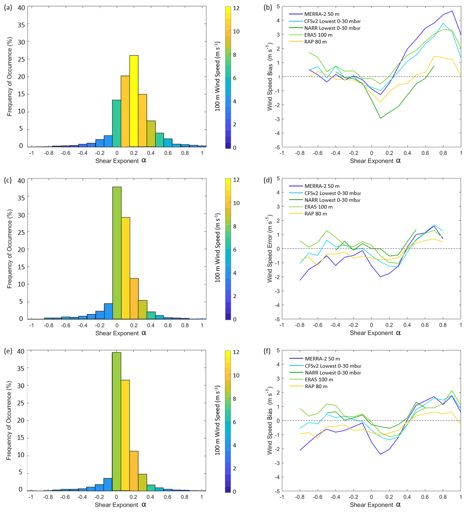
Figure 9Distribution of shear exponent α at (a) Humboldt, (c) Morro Bay during the overlapping Humboldt period, and (e) Morro Bay during the full seasonal cycle, colored by observed 100 m wind speed. Average hub height wind speed bias according to α at (b) Humboldt, (d) Morro Bay during the overlapping Humboldt period, and (d) Morro Bay during the full seasonal cycle.
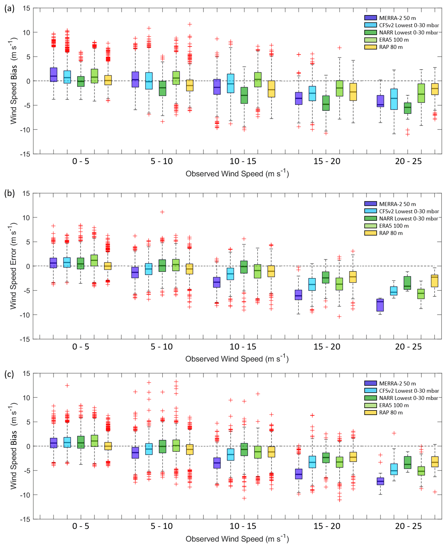
Figure 10Model wind speed bias according to observed wind speed at (a) Humboldt, (b) Morro Bay during the overlapping Humboldt period, and (c) Morro Bay during the full seasonal cycle.
3.4 Model performance according to wind speed class
At both buoy deployment locations, the models are found to slightly overestimate the slowest observed wind speed and strongly underestimate the fastest observed wind speeds (Fig. 10). At Humboldt, the models produce biases ranging from near 0 (NARR) to 1.4 m s−1 (MERRA-2) for observed wind speeds between 0 and 5 m s−1. At Morro Bay, the models produce biases ranging from near 0 (RAP) to 1.1 m s−1 (ERA5) for observed wind speeds between 0 and 5 m s−1, during the overlapping Humboldt period and the full seasonal cycle. Given typical turbine cut-in speeds around 3 to 5 m s−1, this result indicates that the models may underrepresent the fraction of a wind farm life cycle when the turbines are unable to produce power due to low wind speeds.
Wind speeds between 5 and 10 m s−1 represent the steepest portion of a typical turbine power curve, and the models produce biases closest to 0 m s−1 for this range (Fig. 10). At Humboldt, the model biases range from −1.5 (NARR) to 0.6 m s−1 (ERA5), and at Morro Bay the model biases range from −1.3 (MERRA-2) to 0.1 m s−1 (ERA5). Simulating power production using the National Renewable Energy Laboratory (NREL) 6 MW reference turbine (Musial et al., 2019), a wind speed bias of ± 1 m s−1 translates to discrepancies in gross capacity factor ranging from 8 to 23 percentage points when a turbine is operating at wind speeds between 5 and 10 m s−1.
At wind speeds near or at the top of typical turbine power curves (> 10 m s−1), the models exhibit a trend of increasingly negative bias with increasing observed wind speeds (Fig. 10). For all observed winds speeds exceeding 10 m s−1 at Humboldt, the average model rotor-level wind speed biases range from −3.5 (NARR) to −0.3 m s−1 (ERA5). For the fastest wind speed class at Humboldt, from 20 to 25 m s−1, the biases range from −5.8 (NARR) to −1.7 m s−1 (RAP). For all observed winds speeds exceeding 10 m s−1 at Morro Bay, the average model rotor-level wind speed biases range from −3.8 (MERRA-2) to −0.9 m s−1 (NARR) during the overlapping Humboldt period and from −4.0 (MERRA-2) to −1.3 m s−1 (NARR) during the full seasonal cycle. For the fastest wind speed class at Morro Bay, from 20 to 25 m s−1, the biases range from −8.0 (MERRA-2) to −2.3 m s−1 (RAP) during the overlapping Humboldt period and from −7.0 (MERRA-2) to −3.1 m s−1 (RAP) during the full seasonal cycle. One of the reasons for large deviations within various models during high wind speeds could be due to unfavorable parameterization schemes used within the models for offshore conditions. For surface roughness calculations, MERRA-2 uses the Large and Pond (1981) parameterization scheme (Helfand and Schubert, 1995), which is known for significant deviations in offshore conditions (Edson et al., 2013). Since the surface roughness estimates are used within MOST for estimating the winds within the lowest few hundred meters, higher error in surface roughness directly correlates to higher error in wind speed estimates. At very high wind speeds (greater than 25 m s−1), surface roughness no longer increases with wind speed and improper parameterizations can cause larger errors in models (Donelan et al., 2004). Translating these findings to wind farm expectations, the large biases produce minimal discrepancies in simulated gross capacity factor when turbines are operating at wind speeds near the center of the flat top portion of the power curve. The biases become significant for wind speeds near the edges of the flat top of the power curve, however, and can lead to misrepresentation of the fraction of a wind farm life cycle spent at peak production. The biases can also lead to misrepresentation of the portion of a wind farm life cycle spent beyond turbine cut-out or in the state when turbine power slowly derates during very high wind speeds, depending on the turbine technology.
There could be several compounding reasons for such inconsistencies. It is likely that the model underestimation of wind speed in the highest observed wind speed class is due to the coarse resolution of the models and the small spatial scale of these features. The reason for the model overestimation for the lowest observed wind speed class is less clear, but it could be related to unresolved wind direction variability in low-speed conditions (which would tend to reduce the observed vector-averaged wind speed) or to biases in the model parameterization of wave roughness in low-speed conditions.

Figure 12Seasonal and diurnal wind speed bias when comparing (a, e) MERRA-2 and observations at 50 m, (b, f) the CFSv2 lowest 0–30 mbar layer above sea level and observations at 80 m, (c, g) ERA5 and observations at 100 m, and (d, h) RAP and observations at 80 m at Humboldt and Morro Bay.
3.5 Seasonal and diurnal trends in model error
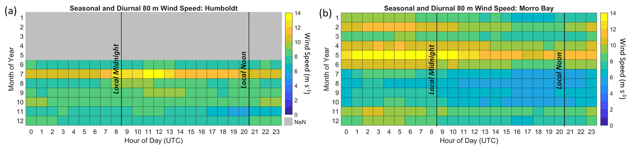
The accuracy of model representation of the observed California coast rotor-level winds varies according to season and time of day. The Morro Bay buoy provides observations over an entire seasonal cycle, identifying that the fastest rotor-level wind speeds occur between the months of November and June (Fig. 11b). Comparing the observations with the models reveals that MERRA-2, CFSv2, ERA5, and RAP strongly underestimate the observed lidar wind speeds between October and June by 2.0, 1.0, 0.8, and 1.0 m s−1, respectively (Fig. 12e–h). During the warm period between July and September, which is characterized by slow wind speeds (Fig. 11b), MERRA-2, CFSv2, and ERA5 produce less negative or even positive biases (−0.5, −0.1, and 0.8 m s−1 on average, respectively), a transition that is particularly pronounced for ERA5. RAP tends to produce consistently negative biases throughout the diurnal cycle between November and May at Morro Bay (−1.2 m s−1) and biases closer to zero between June and October (−0.3 m s−1).
The most pronounced diurnal patterns in model bias occur during the summer months at Morro Bay (Fig. 12e–h). At the buoy locations, 08:00 coordinated universal time (UTC) corresponds to local midnight in Pacific standard time (PST) and 20:00 UTC corresponds to local noon in PST. Positive model rotor-level wind speed biases occur in the summer afternoons and persist through the evening. The slowest wind speeds, shown to be correlated with positive wind speed bias (Fig. 10), are present throughout the summer mornings and afternoons at Morro Bay, persisting into the evenings (Fig. 11b). This period also coincides with little to no wind shear and unstable atmospheric conditions.
At Humboldt, the models similarly show strong diurnal patterns in rotor-level wind speed bias during the warmer months for MERRA-2, CFSv2, and ERA5 (Fig. 12a–d), though a full seasonal analysis is limited due to data availability (Fig. 2a). From June through October, MERRA-2, CFSv2, and ERA5 strongly overestimate the observed rotor-level wind speeds by 1.2, 0.9, and 1.2 m s−1, respectively, from local noon to midnight PST. During the same months but for the hours after midnight through the morning, MERRA-2 and CFSv2 underestimate the observed wind speeds at Humboldt by 0.4 m s−1, while ERA5 overestimates the observed wind speeds by 0.3 m s−1. RAP shows a much subtler diurnal trend in rotor-level wind speed bias at Humboldt (Fig. 12d).

In order to visualize the trends in model error according to time of day at Morro Bay and Humboldt, the seasonal and diurnal patterns in rotor-level wind speed are presented in Figs. 13 and 14. A consistent diurnal pattern is present at Morro Bay throughout the year, with the fastest wind speeds occurring in the evening and at night and the slowest wind speeds occurring in the morning (Fig. 13). All models capture the diurnal trend throughout the year at Morro Bay but consistently underestimate the observations.
Inability of the models to predict the marine boundary layer depth can cause significant overestimation or underestimation of winds within the region. Shallow marine atmospheric boundary layer depths are typically observed during summer months and could be one of the reasons for larger deviations between models and observations. Larger atmospheric boundary layer depths tend to be associated with more positive surface heat fluxes to the atmosphere, which are in turn associated with large surface–air temperature differentials. Over land, this is primarily driven by the response of surface temperature to local solar heating, which is more intense in summer. Over the ocean, however, the local change in air temperature in the summer tends to be greater than the ocean temperature change, which may even be negative when upwelling is present. Therefore, in summer the atmospheric stability actually tends to be increased relative to winter, leading to less positive (or even negative) surface heat fluxes and shallower atmospheric boundary layer depths. The summertime position of the North Pacific subtropical high pressure causes the marine atmospheric boundary layer to slope downward near the taller mountainous California coast, trapping the boundary layer between the surface, the mountains, and the inversion (Dorman et al., 1999; Ström and Tjernström, 2004). The inversion base in this region can range from 100 to 800 m during the summer but typically is observed between 300 and 400 m (Dorman, 1985, 1987; Juliano et al., 2017).
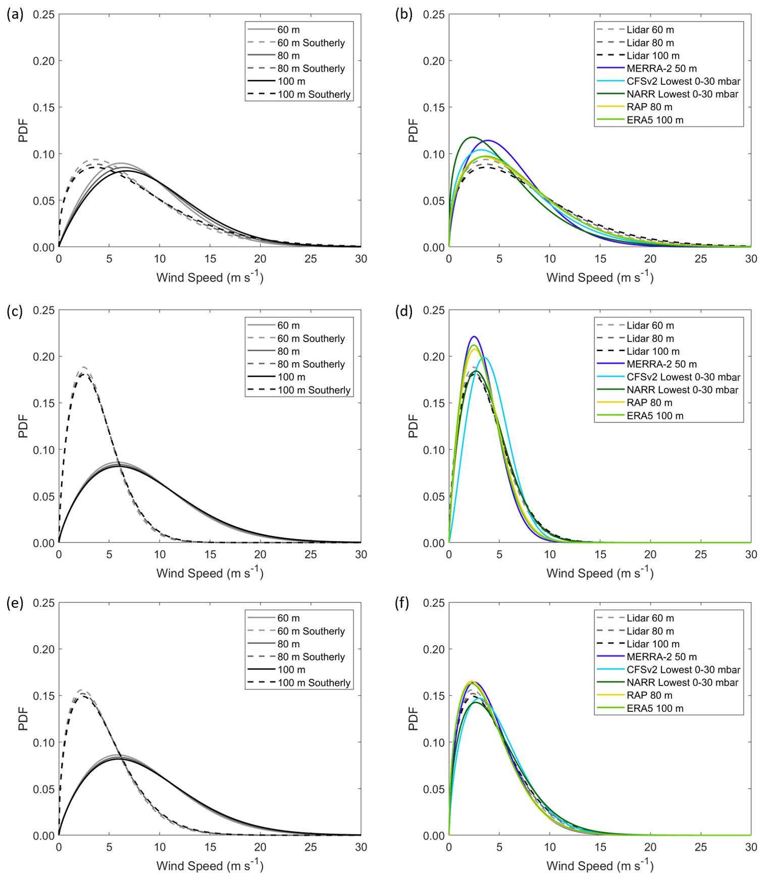
Figure 15(a) Weibull fits to observed wind speeds for all wind directions (solid) and southerly flow (120–240∘) (dashed) at Humboldt. (b) Weibull fits to observed wind speeds for all wind directions (solid) and southeasterly flow (90–210∘) (dashed) at Morro Bay during (c) the overlapping Humboldt period and (e) the entire seasonal cycle. (b) Weibull fits to observed (dashed) and modeled (solid) wind speeds during southerly observed flow at Humboldt. Weibull fits to observed (dashed) and modeled (solid) wind speeds during southerly observed flow at Morro Bay during (d) the overlapping Humboldt period and (f) the full seasonal cycle, respectively.
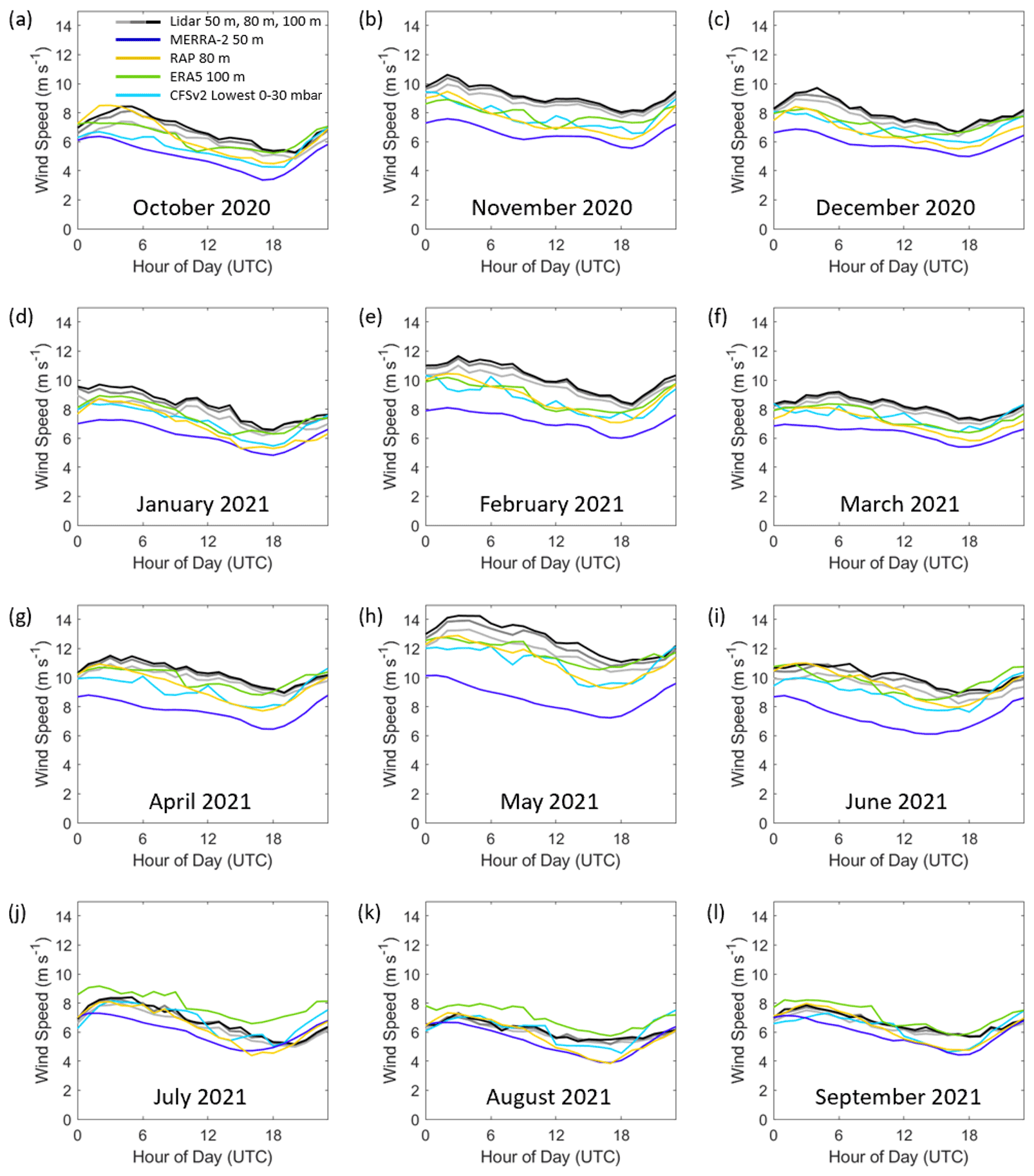
At Humboldt, the diurnal pattern in rotor-level wind speed changes notably throughout the year. The diurnal patterns in modeled and observed wind speed at Humboldt align well for the month of November (Fig. 14b), with all sources showing the wind speed minimum occurring around local noon PST (20:00 UTC) and static winds throughout the evening and night. Contrastingly, there is poor correlation between the modeled and observed diurnal wind speeds during the month of July at Humboldt (Fig. 14e). The lidar data show a pattern of static winds in the afternoon and evening that begin to increase just before local midnight PST (08:00 UTC) to a maximum around 03:00 PST (12:00 UTC), followed by a steady decrease throughout the morning hours (Figs. 11a and 14e). MERRA-2 shows the opposite diurnal pattern in July, with faster winds occurring during the afternoon and evening and slower winds occurring at night. RAP displays little variation in simulated wind speed according to the diurnal cycle, with a gentle minimum occurring in the afternoon. The CFSv2 winds show stronger variation according to the four daily runtimes at 00:00, 06:00, 12:00, and 18:00 UTC than according to the overall diurnal cycle. Like RAP, ERA5 displays little variation in wind speed according to time of day, with the exceptions of two sharp drops in the wind speed that occur 12 h apart at 10:00 UTC (02:00 PST) and 22:00 UTC (14:00 PST).
3.6 Model performance during West Coast weather phenomena
The period of October 2020–September 2021 was not marked by many significant atmospheric or geologic events along the coast of California. The Humboldt and Morro Bay buoys were not impacted by any Pacific tropical storms or significant earthquakes. The Morro Bay buoy was impacted by several weather events, wind reversals associated with the Santa Ana winds, and an atmospheric river, and the following discussion provides insight into model wind speed performance during these events.
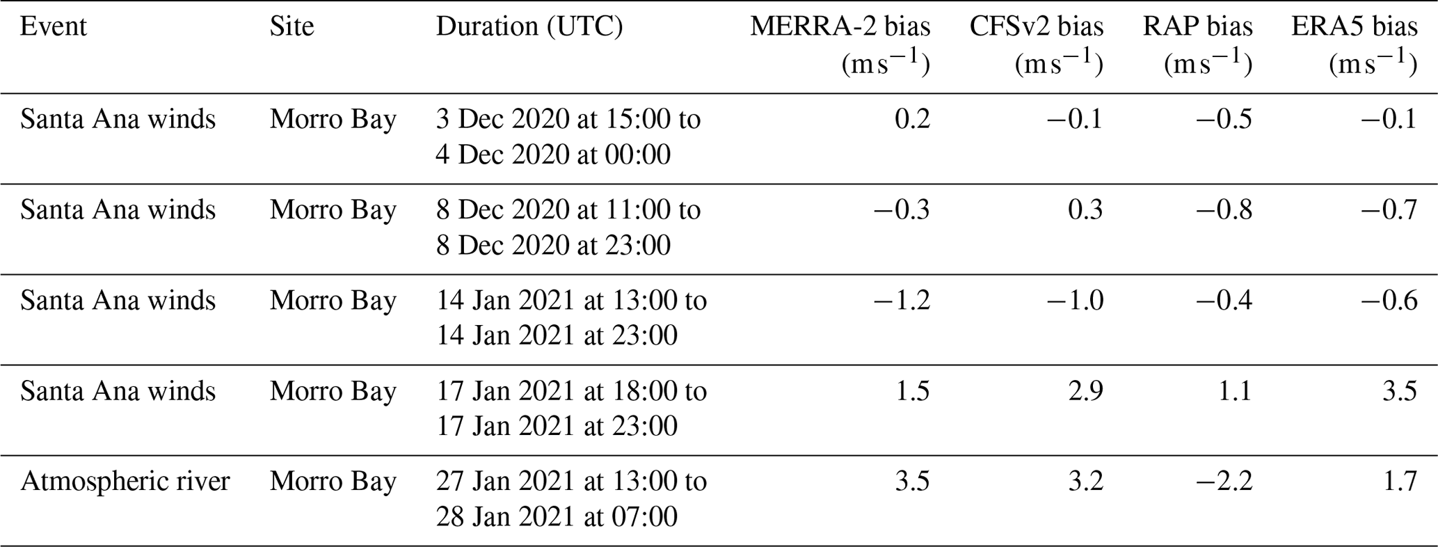
Table 3Model bias during Pacific coast weather events during the lidar buoy deployments.
While the US West Coast is dominated by northerly and northwesterly winds (Fig. 1), abrupt reversals to southerly and southeasterly flow are known to occur. Bond et al. (1996) classify such wind reversals as coastally trapped, associated with ageostrophic flow that is confined to the coastal zone, and synoptic, which is the result of landfalling frontal systems. The observations from the lidar buoys show drastically reduced rotor-level wind speeds at the central California Morro Bay site and slightly reduced rotor-level wind speeds at the northern California Humboldt site during southerly winds relative to the average speeds at each location (Fig. 15a, c, and e), supporting the trend of increasing wind speeds with increasing latitude during reversals noted by Bond et al. (1996). Wind reversal events comprise 11 % of the entire Morro Bay deployment and 11 % and 22 % of the Morro Bay and Humboldt deployments, respectively, during the overlapping data recovery periods of 1 October 2020–27 December 2020 and 25 May 2021–30 September 2021.
The models underestimate the observed rotor-level wind speeds at the northern California Humboldt site during southerly wind events. MERRA-2, ERA5, and CFSv2 produce biases near −1 m s−1 during wind reversals, which are larger than their deployment-wide biases of 0.0, 0.4, and −0.1 m s−1, respectively. The RAP and NARR biases during wind reversals, −0.6 and −1.7 m s−1, respectively, are more positive relative to their deployment-wide biases of −0.9 and −1.9 m s−1, respectively.
At the central California Morro Bay site, all five models exhibit a reduction in rotor-level wind speed bias magnitude during wind reversals relative to their respective deployment-wide biases. MERRA-2, ERA5, and RAP underestimate the southerly observed rotor-level wind speeds during reversals with biases of −0.1, −0.4, and −0.3 m s−1, respectively, reduced from their deployment-wide biases of −1.7, −0.4, and −0.8 m s−1, respectively. CFSv2 and NARR overestimate the southerly observed rotor-level wind speeds at Morro Bay by 0.3 and 0.3 m s−1, respectively, a sign transition from their deployment-wide biases of −0.8 and −0.3 m s−1, respectively.
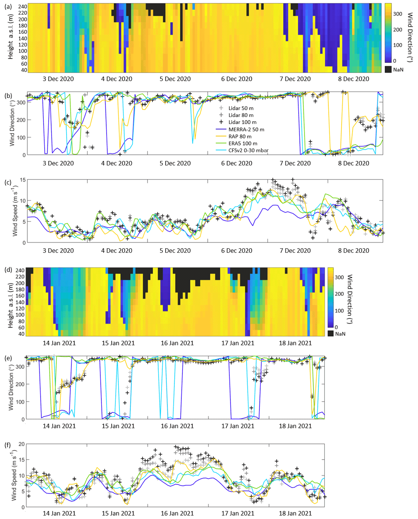
Figure 16(a, d) Observed wind direction, (b, e) observed and modeled rotor-level wind direction, and (c, f) observed and modeled rotor-level wind speed at Morro Bay.
One meteorological phenomenon that can result in atypical wind directions along the central and southern California coasts are the Santa Ana winds. These warm, dry downslope winds are most frequently present in December and January (Guzman-Morales et al., 2016) and occur when a Great Basin high is present simultaneously with a surface low-pressure system offshore (Raphael, 2003). This develops a counterclockwise circulation zone offshore, creating a flow reversal at the buoy location. Four occasions of wind reversals during Santa Ana pressure setups are noted in the Morro Bay buoy record (Fig. 16).
The first event, 3 December 2020 at 15:00 UTC–4 December 2020 at 00:00 UTC, is characterized by very low wind speeds (< 5 m s−1). During this period, RAP is the best performing model at capturing the observed southerly winds at Morro Bay (Fig. 16b), likely due to its high spatial resolution. ERA5 and CFSv2 remain northerly throughout the duration of the event, while MERRA-2 steadily transitions through the entire directional spectrum. The rotor-level wind speed biases during this event are small, ranging from −0.5 (RAP) to 0.2 m s−1 (MERRA-2) (Fig. 16c, Table 3). NARR is excluded from the Santa Ana case study analysis due to the reduced sample size resulting from its coarser temporal resolution.
Low wind speeds similarly characterize the second event, 8 December 2020 at 11:00–23:00 UTC. RAP is the only model that accurately captures the southerly flow event (Fig. 16b). MERRA-2, CFSv2, and ERA5 remain northerly to northeasterly throughout the duration of the event. The rotor-level wind speed biases range from −0.8 (RAP) to 0.3 m s−1 (CFSv2) (Table 3).
Relatively higher wind speeds that correspond to the steep portion of a typical turbine power curve (4–9 m s−1) are observed during the third event, 14 January 2021 at 13:00–23:00 UTC. Similar to the prior events, RAP is successful at capturing the flow reversal (Fig. 16e), while the remaining models consistently show northerly flow. The rotor-level wind speed biases are more pronounced, ranging from −1.2 (MERRA-2) to −0.4 m s−1 (RAP) (Table 3).
The fourth event, 17 January 2021 at 18:00–23:00 UTC, is characterized by low observed rotor-level speeds that follow a steep decline following a burst of wind exceeding 10 m s−1 (Fig. 16f) associated with damaging winds along the central California coast (National Weather Service, 2022). None of the models capture the short-lived wind reversal and instead remain consistently northerly (Fig. 16e). The models substantially overestimate the observed rotor-level wind speeds, with biases ranging from 1.1 (RAP) to 3.5 m s−1 (ERA5) (Table 3). Notably, none of the models capture the observed burst of wind and the subsequent steep decline in the observed wind speed prior to the wind reversal event, indicating model challenges in resolving atmospheric phenomena that change over periods of short duration.

Figure 17(a) Observed pressure, (b) observed air and sea temperature, (c) observed wind speed, and (d) observed and modeled wind speed at the Morro Bay buoy during the January 2021 western US atmospheric river event.
A powerful atmospheric river event impacted the western US from 26–29 January 2021 (Weather Prediction Center, 2022). Heavy mountain snow and flooding were recorded across California. At the Morro Bay buoy, the recorded low pressure reached a minimum around the 27–28 January transition, an event that coincided with rapid shifts in the temperature, wind speed, and wind direction (Fig. 17).
From 13:00–21:00 UTC on 27 January, the rotor-level winds transition from southerly to easterly flow, accompanied by wind speeds ranging from 9–13 m s−1. At 22:00 UTC, the winds drastically shift to westerly and reduce to ∼ 5 m s−1. At 23:00 UTC, the wind direction begins to transition back to southerly flow, and by midnight UTC on 28 January, the rotor-level wind speeds spike to 22 m s−1. The enhanced wind speeds sustain for a period of 3 h before rapidly decreasing to ∼ 6 m s−1.
MERRA-2 and CFSv2 fail to capture the rapid changes in wind direction, remaining southerly throughout the duration of the event. ERA5 captures the initial shift to easterly winds, albeit several hours early, but subsequently remains southerly throughout the remainder of the event, missing the drastic shift to westerly winds. Only RAP captures the entire transition from southerly to easterly to westerly and back to southerly winds and with an accuracy of ± 1 h. In terms of wind speed, only RAP captures the rapidly changing wind pattern throughout the event, though with a low bias of −2.2 m s−1 (Table 3). MERRA-2, CFSv2, and ERA5 fail to capture the rapid wind speed transitions, instead producing gently sloped peaks in the modeled wind speed that occur before (MERRA-2) or after (CFSv2, ERA5) the observed wind speed peak. This mischaracterization leads to substantial overestimation during the atmospheric river event, with rotor-level wind speed biases of 3.5, 3.2, and 1.7 m s−1 for MERRA-2, CFSv2, and ERA5, respectively (Table 3).
As offshore wind plays an increasing role in the US and global energy portfolios, the need to validate the models that support long-term wind resource characterization in areas of offshore wind development interest similarly increases. The DOE lidar buoys provide essential observations for validation at the spatial scales most relevant for offshore wind: over the water and at rotor layer height. The recent deployments of the lidar buoys off the coast of California in two areas of interest for offshore wind development, Humboldt and Morro Bay, reveal a trend of model underestimation of the observed hub height wind speeds. At the northern California Humboldt location, MERRA-2 and CFSv2 yield the smallest rotor-level wind speed biases, near zero, while NARR produces the largest magnitude bias of −1.9 m s−1. Contrastingly, at the central California Morro Bay location during the overlapping Humboldt period, MERRA-2 produces the largest-magnitude rotor-level wind speed bias of −1.3 m s−1 (−1.6 m s−1 during the full Morro Bay deployment), while NARR and ERA5 yield the smallest biases of 0 m s−1 (−0.3 m s−1) and −0.2 m s−1 (−0.4 m s−1), respectively.
For the direct comparisons of model level to lidar level, RAP, the model with the highest spatial resolution, provides the lowest CRMSEs (2.3 m s−1 at Humboldt, 1.7 m s−1 at Morro Bay during the overlapping Humboldt period, 1.7 m s−1 at Morro Bay during the full deployment) and the highest correlations (0.88, 0.93, 0.94). MERRA-2, the coarsest model, produces the highest CRMSEs (2.7, 2.4, 2.6 m s−1) and lowest correlations (0.79, 0.85, 0.86). The lowest 0–30 mbar layer above sea level from CFSv2, NARR, and RAP provides an appropriate representation of 80 m wind speeds based on correlations of 0.82 or greater along with biases and CRMSEs of similar magnitude to those produced based on the direct level comparisons.
An investigation into the conditions leading to large simulation error reveals model mishandling of the summer diurnal pattern in the wind speed at the northern Humboldt location, though the diurnal pattern in cooler months is well captured. Trends in reanalysis wind speed bias according to atmospheric stability are location-dependent, with model underestimation of the observed wind speeds during near-neutral conditions at both sites but overestimation of the observed winds during stable conditions at Humboldt and unstable conditions at Morro Bay. Model bias varies strongly according to observed wind speed class and weakly according to significant wave height. At Humboldt, MERRA-2, ERA5, and CFSv2 produced larger-magnitude biases during wind reversal events relative to the deployment-wide biases, while at Morro Bay all models experience a reduction in bias magnitude during wind reversals. For wind reversals at Morro Bay resulting from the Santa Ana winds, RAP is the best performing model at capturing directional shifts.
The upcoming effort for continuing this research begins with the re-examination of model performance at Humboldt once an entire seasonal cycle is available at that location. Next, model performance can be analyzed according to additional atmospheric and oceanic phenomena of interest to the wind energy community, such as low-level jets (observed at the Morro Bay buoy location). Understanding the physical processes leading to the changing biases in the diurnal cycle seen throughout the year will be important for guiding the use of both reanalyses and understanding forecasts for these offshore wind locations. Finally, the observations from the California deployments of the DOE lidar buoys will be used to validate the performance of coupled wind–wave simulations of offshore winds (Gaudet et al., 2022).
The data utilized in this study are freely and publicly available. The lidar buoy observations are available from the U.S. Department of Energy at https://doi.org/10.21947/1783807 (U.S. Department of Energy, 2022a) and https://doi.org/10.21947/1783809 (U.S. Department of Energy, 2022b). NASA provides MERRA-2 through the Goddard Earth Sciences Data and Information Services Center at https://gmao.gsfc.nasa.gov/reanalysis/MERRA-2/data_access/ (NASA, 2022). CFSv2 and NARR are accessed via the Research Data Archive provided by the National Center for Atmospheric Research at https://rda.ucar.edu/ (NCAR, 2022). ERA5 is available through the Copernicus Climate Change Service Climate Data Store at http://cds.climate.copernicus.eu (Copernicus, 2022). RAP is available for download at NOAA's National Centers for Environmental Information at http://ncei.noaa.gov (NCEI, 2022). Data from neighboring buoys are provided by NOAA's National Data Buoy Center at https://www.ndbc.noaa.gov/ (NDBC, 2021). Satellite data from the collection are available at http://thredds.aodn.org.au/thredds/catalog/IMOS/SRS/Surface-Waves/Wave-Wind-Altimetry-DM00/catalog.html (Ribal and Young, 2019).
For convenience, paired time series of wind data from the model and observations at the Humboldt location are provided at https://doi.org/10.21947/1839076 (U.S. Department of Energy, 2022c), along with processing scripts. Paired time series of wind data from the model and observations at the Morro Bay location are provided at https://doi.org/10.21947/1839076 (U.S. Department of Energy, 2022c), along with processing scripts.
LS accessed and processed the data and led the data analysis with significant contributions from RK, GGM, and BG. RK, AM, and WS led the project and provided essential direction for this research. WG and ZY provided additional valuable feedback and guidance for the project. MP and RN were instrumental in the acquisition and processing of the lidar buoy observations.
The contact author has declared that none of the authors has any competing interests.
Publisher's note: Copernicus Publications remains neutral with regard to jurisdictional claims in published maps and institutional affiliations.
This work was authored by the Pacific Northwest National Laboratory, operated for the U.S. Department of Energy by Battelle (contract no. DE-AC05-76RL01830). Additionally, the authors would like to thank Shannon Davis and Mike Derby at the U.S. Department of Energy Wind Energy Technologies Office for funding this research and Doug Boren, Necy Sumait, and Frank Pendleton at the U.S. Department of the Interior Bureau of Ocean Energy Management for funding the Humboldt and Morro Bay deployments. The authors would also like to thank Julia Flaherty and Catie Himes for reviewing the preliminary draft of the article. The authors are grateful for the helpful edits and suggestions provided by the anonymous reviewers that substantially improved this paper.
This research has been supported by the U.S. Department of Energy Wind Energy Technologies Office (grant no. DE-AC05-76RL01830).
This paper was edited by Raimund Rolfes and reviewed by two anonymous referees.
Ao, C. O., Waliser, D. E., Chan, S. K., Li, J-L., Tian, B., Xie, F., and Mannucci, A. J.: Planetary boundary layer heights from GPS radio occultation refractivity and humidity profiles, J. Geophys. Res.-Atmos., 117, D16117, https://doi.org/10.1029/2012JD017598, 2012.
Beljaars, A. C. M. and Holtslag, A. A. M.: Flux parameterization over land surfaces for atmospheric models, J. Appl. Meteorol. Clim., 30, 327–341, https://doi.org/10.1175/1520-0450(1991)030%3C0327:FPOLSF%3E2.0.CO;2, 1991.
Benjamin, S. G., Weygandt, S. S., Brown, J. M., Hu, M., Alexander, C. R., Smirnova, T. G., Olson, J. B., James, E. P., Dowell, D. C., Grell, G. A., Lin, H., Peckham, S. E., Smith, T. L., Moninger, W. R., Kenyon, J. S., and Manikin, G. S.: A North American hourly assimilation and model forecast cycle: The Rapid Refresh, Mon. Weather Rev., 144, 1669–1694, https://doi.org/10.1175/MWR-D-15-0242.1, 2016.
Benjamin, S. G., James, E. P., Brown, J. M., Szoke, E. J., Kenyon, J. S., and Ahmadov, R.: Diagnostic fields developed for hourly updated NOAA weather models, NOAA Technical Memorandum OAR GSL-66, Earth Systems Research Laboratory, National Oceanic and Atmospheric Administration, Boulder, CO, 58 pp. https://doi.org/10.25923/98fy-xx71, 2020.
Bond, N. A., Mass, C. F., and Overland, J. E.: Coastally trapped wind reversals along the United States west coast during the warm season. Part I: Climatology and temporal evolution, Mon. Weather Rev., 124, 3, 430, 1996.
Businger, J. A., Wyngaard, J. C., Izumi, Y., and Bradley, E. F.: Flux profile relationships in the atmospheric surface layer, J. Atmos. Sci., 28, 181–189, https://doi.org/10.1175/1520-0469(1971)028%3C0181:FPRITA%3E2.0.CO;2, 1971.
Copernicus: Climate Data Store, https://cds.climate.copernicus.eu/, last access: 3 January 2022.
de Assis Tavares, L. F., Shadham, M., de Freitas Assad, L. P., and Estefen, S. F.: Influence of the WRF Model and Atmospheric Reanalysis on the Offshore Wind Resource Potential and Cost Estimation: A Case Study for Rio De Janeiro State, SSRN, 3895673, https://doi.org/10.2139/ssrn.3895673, 2021.
Donelan, M. A., Haus, B. K., Reul, N., Plant, W. J., Stiassnie, M., Graber, H. C., Brown, O. B., and Saltzman, E. S.: On the limiting aerodynamic roughness of the ocean in very strong winds, Geophys. Res. Lett., 13, L18306, https://doi.org/10.1029/2004GL019460, 2004.
Dong, C., Huang, G., and Cheng, G.: Offshore wind can power Canada, Energy, 236, 121422, https://doi.org/10.1016/j.energy.2021.121422, 2021.
Dorman, C. E.: Evidence of Kelvin Waves in California's Marine Layer and Related Eddy Generation, Mon. Weather Rev., 113, 827–839, https://doi.org/10.1175/1520-0493(1985)113%3C0827:EOKWIC%3E2.0.CO;2, 1985.
Dorman, C. E.: Possible role of gravity currents in northern California's coastal summer wind reversals, J. Geophys. Res.-Oceans, 92, 1497–1506, https://doi.org/10.1029/JC092iC02p01497, 1987.
Dorman, C. E. and Winant, C. D.: Buoy observations of the atmosphere along the west coast of the United States, 1981–1990, J. Geophys. Res.-Oceans, 100, 16029–16044, https://doi.org/10.1029/95JC00964, 1995.
Dorman, C. E., Rogers, D. P., Nuss, W., and Thompson, W. T.: Adjustment of the Summer Marine Boundary Layer around Point Sur, California, Mon. Weather Rev., 127, 2143–2159, https://doi.org/10.1175/1520-0493(1999)127%3C2143:AOTSMB%3E2.0.CO;2, 1999.
Dyer, A. J.: A review of flux-profile relationships, Bound.-Lay. Meteorol., 7, 363–372, 1974.
Edson, J. B., Jampana, V., Weller, R. A., Bigorre, S. P., Plueddemann, A. J., Fairall, C. W., Miller, S. D., Mahrt, L., Vickers, D., and Hersbach, H.: On the exchange of momentum over the open ocean, J. Phys. Oceanogr., 43, 1589–1610, https://doi.org/10.1175/JPO-D-12-0173.1, 2013.
Fairall, C. W., Bradley, E. F., Rogers, D. P., Edson, J. B., and Young, G. S.: Bulk parameterization of air–sea fluxes for tropical ocean–global atmosphere coupled-ocean atmosphere response experiment, J. Geophys. Res.-Oceans, 101, 3747–3764, https://doi.org/10.1029/95JC03205, 1996.
Fernandes, I. G., Pimenta, F. M., Saavedra, O. R., and Silva, A. R.: Offshore Validation of ERA5 Reanalysis with Hub Height Wind Observations of Brazil, 2021 IEEE PES Innovative Smart Grid Technologies Conference – Latin America (ISGT Latin America), 15–17 September 2021, Virtual, 1–5, https://doi.org/10.1109/ISGTLatinAmerica52371.2021.9542993, 2021.
Gaudet, B. J., García Medina, G., Krishnamurthy, R., Shaw, W. J., Sheridan, L. M., Yang, Z., Newsom, R. K., and Pekour, M.: Evaluation of coupled wind / wave model simulations of offshore winds in the Mid-Atlantic Bight using lidar-equipped buoys, Mon. Weather Rev., 150, 1377–1395, https://doi.org/10.1175/MWR-D-21-0166.1, 2022.
Gelaro, R., McCarty, W., Suárez, M. J., Todling, R., Molod, A., Takacs, L., Randles, C. A., Darmenov, A., Bosilovich, M. G., Reichle, R., Wargan, K., Coy, L., Cullather, R., Draper, C., Akella, S., Buchard, V., Conaty, A., da Silva, A. M., Gu, W., Kim, G-K., Koster, R., Lucchesi, R., Merkova, D., Nielsen, J. E., Partyka, G., Pawson, S., Putnam, W., Rienecker, M., Schubert, S. D., Sienkiewicz, M., and Zhao, B.: The Modern-Era Retrospective Analysis for Research and Applications, Version 2 (MERRA-2), J. Climate, 30, 5419–5454, https://doi.org/10.1175/JCLI-D-16-0758.1, 2017.
Gorton, A. M. and Shaw, W. J.: Advancing Offshore Wind Resource Characterization Using Buoy-Based Observations, Mar. Technol. Soc. J., 54, 37–43, https://doi.org/10.4031/MTSJ.54.6.5, 2020.
Grachev, A. A. and Fairall, C. W.: Dependence of the Monin-Obukhov Stability Parameter on the Bulk Richardson Number over the Ocean, J. Appl. Meteorol. Clim., 36, 406–414, https://doi.org/10.1175/1520-0450(1997)036%3C0406:DOTMOS%3E2.0.CO;2, 1997.
Guzman-Morales, J., Gershunov, A., Theiss, J., Li, H., and Cayan, D.: Santa Ana Winds of Southern California: Their climatology, extremes, and behavior spanning six and a half decades, Geophys. Res. Lett., 43, 2827–2834, https://doi.org/10.1002/2016GL067887, 2016.
Haack, T. and Burk, S. D.: Summertime Marine Refractivity Conditions along Coastal California, J. Appl. Meteorol. Clim., 40, 673–687, https://doi.org/10.1175/1520-0450(2001)040%3C0673:SMRCAC%3E2.0.CO;2, 2001.
Haus, B. K., Ortiz-Suslow, D. G., Doyle, J. D., Flagg, D. D., Graber, H. C., MacMahan, J., Shen, L., Wang, Q., Williams, N. J., and Yardim, C.: CLASI: Coordinating innovative observations and modeling to improve coastal environmental prediction systems, B. Am. Meteorol. Soc., https://doi.org/10.1175/BAMS-D-20-0304.1, in press, 2022.
Hayes, L., Stocks, M., and Blakers, A.: Accurate long-term power generation model for offshore wind farms in Europe using ERA5 reanalsysis, Energy, 229, 120603, https://doi.org/10.1016/j.energy.2021.120603, 2021.
Helfand, H. M. and Schubert, S. D.: Climatology of the simulated great plains low-level jet and its contribution to the continental moisture budget of the United States, J. Climate, 8, 784–806, https://doi.org/10.1175/1520- 0442(1995)008<0784:COTSGP>2.0.CO;2, 1995.
Hersbach, H., Bell, B., Berrisford, P., Hirahara, S., Horányi, A., Muñoz-Sabater, J., Nicolas, J., Peubey, C., Radu, R., Schepers, D., Simmons, A., Soci, C., Abdalla, S., Abellan, X., Balsamo, G., Bechtold, P., Biavati, G., Bidlot, J., Bonavita, M., De Chiara, G., Dahlgren, P., Dee, D., Diamantakis, M., Dragani, R., Flemming, J., Forbes, R., Fuentes, M., Geer, A., Haimberger, L., Healy, S., Hogan, R. J., Hólm, E., Janisková, M., Keeley, S., Laloyaux, P., Lopez, P., Lupu, C., Radnoti, G., de Rosnay, P., Rozum, I., Vamborg, F., Villaume, S., and Thépaut, J.-N.: The ERA5 Global Reanalysis, Q. J. Roy. Meteor. Soc., 146, 1999–2049, https://doi.org/10.1002/qj.3803, 2020.
Jani, H. K., Nagababu, G., Patel, R. P., and Kachhwaha, S. S.: Evaluation of meteorological and reanalysis wind data for the offshore wind resource assessment, 12th International Conference on Thermal Engineering: Theory and Applications, 23–26 February 2019, Gandhinagar, India, https://journals.library.ryerson.ca/index.php/ictea/article/download/1125/1268 (last access: 17 October 2022), 2019.
Juliano, T. W., Parish, T. R., Rahn, D. A., and Leon, D. C.: An Atmospheric Hydraulic Jump in the Santa Barbara Channel, J. Appl. Meteorol. Clim., 56, 2981–2998, https://doi.org/10.1175/JAMC-D-16-0396.1, 2017.
Koračin, D., Dorman, C. E., Lewis, J. M., Hudson, J. G., Wilcox, E. M., and Torregosa, A.: Marine fog: A review, Atmos. Res., 143, 142–175, https://doi.org/10.1016/j.atmosres.2013.12.012, 2014.
Mesinger, F., DiMego, G., Kalnay, E., Mitchell, K., Shafran, P. C., Ebisuzaki, W., Jović, D., Woollen, J., Rogers, E., Berbery, E. H., Ek, M. B., Fan, Y., Grumbine, R., Higgins, W., Li, H., Lin, Y., Manikin, G., Parrish, D., and Shi, W.: North American Regional Reanalysis, B. Am. Meteorol. Soc., 87, 343–360, https://doi.org/10.1175/BAMS-87-3-343, 2006.
Musial, W., Beiter, P., Nunemaker, J., Heimiller, D., Ahmann, J., and Busch, J.: Oregon Offshore Wind Site Feasibility and Cost Study, NREL/TP-5000-74597, National Renewable Energy Laboratory (NREL), Golden, CO (United States), https://doi.org/10.2172/1570430, 2019.
Musial, W., Spitsen, P., Beiter, P., Duffy, P., Marquis, M., Cooperman, A., Hammond, R., and Shields, M.: Offshore Wind Market Report: 2021 Edition, DOE/GO-102021-5614, National Renewable Energy Laboratory (NREL), Golden, CO (United States), https://doi.org/10.2172/1818842, 2021.
NASA: Modern-Era Retrospective analysis for Research and Applications, Version 2, NASA [data set], https://gmao.gsfc.nasa.gov/reanalysis/MERRA-2/data_access/, last access: 3 January 2022.
National Weather Service: Damaging Wind Event, https://www.weather.gov/mtr/Wind_1_17-19_2021, last access: 3 January 2022.
NCAR: Research Data Archive, https://rda.ucar.edu/, last access: 3 January 2022.
NCEI: National Centers for Environmental Information, https://www.ncei.noaa.gov/, last access: 3 January 2022.
NDBC: National Oceanic and Atmospheric Administration's National Data Buoy Center, NDBC [data set], https://www.ndbc.noaa.gov/, last access: 23 November 2021.
Nehzad, M., Neshat, M., Groppi, D., Marzialetti, P., Heydari, A., Sylaios, G., and Astiaso Garcia, D.: A primary offshore wind farm site assessment using reanalysis data: a case study for Samothraki island, Renew. Energ., 172, 667–679, https://doi.org/10.1016/j.renene.2021.03.045, 2021.
Optis, M., Monahan, A., and Bosveld, F. C.: Limitations and breakdown of Monin-Obukhov similarity theory for wind profile extrapolation under stable stratification, Wind Energy, 19, 1053–1072, https://doi.org/10.1002/we.1883, 2015.
Parish, T. R.: Forcing of the Summertime Low-Level Jet along the California Coast, J. Appl. Meteorol. Clim., 39, 2421–2433, https://doi.org/10.1175/1520-0450(2000)039%3C2421:FOTSLL%3E2.0.CO;2, 2000.
Parish, T. R., Rahn, D. A., and Leon, D. C.: Aircraft measurements and numerical simulations of an expansion fan off the California coast, J. Appl. Meteorol. Clim., 55, 2053–2062, https://doi.org/10.1175/JAMC-D-16-0101.1, 2016.
Pronk, V., Bodini, N., Optis, M., Lundquist, J. K., Moriarty, P., Draxl, C., Purkayastha, A., and Young, E.: Can reanalysis products outperform mesoscale numerical weather prediction models in modeling the wind resource in simple terrain?, Wind Energ. Sci., 7, 487–504, https://doi.org/10.5194/wes-7-487-2022, 2022.
Ramon, J., Lledó, L., Torralba, V., Soret, A., and Doblas-Reyes, F. J.: Which global reanalysis best represents near-surface winds?, Q. J. Roy. Meteor. Soc., 145, 3236–3251, https://doi.org/10.1002/qj.3616, 2019.
Raphael, M. N.: The Santa Ana Winds of California, Earth Interact., 7, 1–13, https://doi.org/10.1175/1087-3562(2003)007%3C0001:TSAWOC%3E2.0.CO;2, 2003.
Ribal, A. and Young, I. R.: 33 years of globally calibrated wave height and wind speed data based on altimeter observations, Sci. Data-UK, 6, 77, https://doi.org/10.1038/s41597-019-0083-9, 2019.
Ribal, A. and Young, I. R.: Wind-Wave-Altimetry-DM00, Thredds [data set], http://thredds.aodn.org.au/thredds/catalog/IMOS/SRS/Surface-Waves/Wave-Wind-Altimetry-DM00/catalog.html, last access: 12 October 2021.
Rolinski, T., Capps, S. B., and Zhuang, W.: Santa Ana Winds: A Descriptive Climatology, Weather Forecast., 34, 257–275, https://doi.org/10.1175/WAF-D-18-0160.1, 2019.
Saha, S., Moorthi, S., Wu, X., Wang, J., Nadiga, S., Tripp, P., Behringer, D., Hou, Y. T., Chuang, H. Y., Iredell, M., and Ek, M.: NCEP climate forecast system version 2 (CFSv2) 6-hourly products. Research Data Archive at the National Center for Atmospheric Research, Computational and Information Systems Laboratory, 10, Dp. D61C1TXF, 2011.
Saha, S., Moorthi, S., Wu, X., Wang, J., Nadiga, S., Tripp, P., Behringer, D., Hou, Y-T., Chuang, H-Y., Iredell, M., Ek, M., Meng, J., Yang, R., Peña Mendez, M., van den Dool, H., Zhang, Q., Wang, W., Chen, M., and Becker, E.: The NCEP Climate Forecast System Version 2, J. Climate, 27, 2185–2208, https://doi.org/10.1175/JCLI-D-12-00823.1, 2014.
Severy, M. A. Gorton, A. M., Krishnamurthy, R., and Levin, M. S.: Lidar Buoy Data Dictionary For the 2020–2021 California Deployments, PNNL-30947, Pacific Northwest National Laboratory (PNNL), Richland, WA, USA, https://a2e.energy.gov/data/buoy/buoy.z05.00/attach/pnnl-30937-datadictionary.pdf, last access: 29 November 2021.
Sheridan, L. M., Krishnamurthy, R., Gorton, A. M., Shaw, W. J., and Newsom, R. K.: Validation of Reanalysis-Based Offshore Wind Resource Characterization Using Lidar Buoy Observation, Mar. Technol. Soc. J., 54, 44–61, https://doi.org/10.4031/MTSJ.54.6.13, 2020.
Ström, L. and Tjernström, M.: Variability in the summertime coastal marine atmospheric boundary-layer off California, USA, Q. J. Roy. Meteor. Soc., 130, 423–448, https://doi.org/10.1256/qj.03.12, 2004.
U.S. Department of Energy: Buoy – California – Processed Data, U.S. Department of Energy [data set], https://doi.org/10.21947/1783807, 2022a.
U.S. Department of Energy: Lidar – California – Processed Data, U.S. Department of Energy [data set], https://doi.org/10.21947/1783809, 2022b.
U.S. Department of Energy: Buoy – California – Quality-Controlled Reanalysis and Observational Data – Derived Data, U.S. Department of Energy [code and data set], https://doi.org/10.21947/1839076, 2022c.
Vickers, D. and Mahrt, L.: Observations of non-dimensional wind shear in the coastal zone, Q. J. Roy. Meteor. Soc., 125, 2685–2702, https://doi.org/10.1002/qj.49712555917, 1999.
Wang, Y-H., Walter, R. K., White, C., Farr, H., and Ruttenberg, B. I.: Assessment of surface wind datasets for estimating offshore wind energy along the Central California Coast, Renew. Energ., 133, 343–353, https://doi.org/10.1016/j.renene.2018.10.008, 2019.
Weather Prediction Center: Western U. S. Atmospheric River Event (1/2–1/29), https://www.wpc.ncep.noaa.gov/storm_summaries/event_reviews.php?YYYYMMDD=20210129&product=snow, last access: 3 January 2022.
Wharton, S. and Lundquist, J. K.: Atmospheric stability affects wind turbine power collection, Environ. Res. Lett., 7, 014005, https://doi.org/10.1088/1748-9326/7/1/014005/meta, 2012.