the Creative Commons Attribution 4.0 License.
the Creative Commons Attribution 4.0 License.
 | 04 Feb 2022
Development of a curled wake of a yawed wind turbine under turbulent and sheared inflow
Paul Hulsman
Martin Wosnik
Vlaho Petrović
Michael Hölling
Martin Kühn
Redirecting the wake from an upstream wind turbine by yawing its rotor can reduce the negative impact of the wake on a downstream turbine. The present research investigated wind turbine wake behaviour for three yaw angles at different inflow turbulence levels and shear profiles under controlled conditions. Experiments were conducted using a model wind turbine with 0.6 m diameter (D) in a large wind tunnel. A short-range lidar WindScanner was used to map the wake with high spatial and temporal resolution in vertical, cross-stream planes at different downstream locations and in a horizontal plane at hub height. The lidar WindScanner enabled fast measurements at multiple locations in comparison to the standard hot-wire measurements. The flow structures and the energy dissipation rate of the wake were measured from 1 up to 10 D, and for one inflow case up to 16 D, downstream of the turbine rotor. A strong dependency of the wake characteristics on both the yaw angle and the inflow conditions was observed.
In addition, the curled wake that develops under yaw misalignment due to the counter-rotating vortex pair was more pronounced with a boundary layer (sheared) inflow condition than for uniform inflow with different turbulence levels.
Furthermore, the lidar velocity data and calculated quantities such as the energy dissipation rate compared favourably with hot-wire data from previous experiments with a similar inflow condition and wind turbine model in the same facility, lending credibility to the measurement technique and methodology used here. The results of this measurement campaign provided a deeper understanding of the development of the wake for different yaw angles and inflow conditions which can help improve wake models.
- Article
(12001 KB) - Full-text XML
- BibTeX
- EndNote


Wind turbines within a wind farm can experience significant power losses due to wake effects caused by upstream turbines (Barthelmie et al., 2010) and higher fatigue loads (Thomsen and Sørensen, 1999). Reducing the wake effects of upstream turbines on downstream turbines can potentially increase the power output and decrease the fatigue loads. Currently, one promising technique for mitigating the wake effects is to intentionally steer the wake of the upstream turbine away from the downstream turbine by yawing the rotor of the upstream turbine (Fleming et al., 2014). Recent studies have shown that intentionally steering the wake can increase the annual energy production (Gebraad et al., 2017) and the power output in the free field (Fleming et al., 2019).
However, developing a yaw-control model to change the trajectory of the wake is a challenging task and requires a thorough understanding of the behaviour of the wake under these conditions. Vollmer et al. (2016) concluded from large-eddy simulations that the interrelation between the atmospheric stability and the yaw misalignment has a strong influence on the wake characteristics, thus affecting the wake deficit, trajectory, and wake profile.
Experimental data under controlled conditions are necessary to understand the wake behaviour at different yaw angles and at different inflow conditions, which is critical for developing a reliable and accurate yaw-control model which can be implemented in the field. The potential to redirect the wake has been discussed in several wind tunnel experiments: Medici and Alfredsson (2006), Bastankhah and Porté-Agel (2016), Bartl et al. (2018), and Schottler et al. (2018). One of the earlier studies conducted by Grant et al. (1997) tracked the tip vortices using optical methods downstream of a model turbine. The study indicated the influence of the yaw angle on the tip vortices and thus on the wake expansion and wake deflection. Grant and Parkin (2000) used phase-locked particle image velocimetry (PIV) measurements to measure the circulation within the wake. The measurements found an asymmetry in the wake shape for positive and negative yaw angles. Similar results were obtained by Haans et al. (2005). Medici and Alfredsson (2006) quantified the velocity deficit at multiple downwind locations in the far-wake region using a two‐component hot wire. During their measurements, they observed additional vortex shedding at large yaw angles. Furthermore, they determined that a cross-stream flow component causes the wake to deflect. The PIV measurement campaign conducted by Bastankhah and Porté-Agel (2016) showed an asymmetric flow entrainment in the wake with regard to the mean and turbulent momentum balances. Schottler et al. (2016) investigated the interaction between two model turbines highlighting clear asymmetries of the power output of the downstream turbine between a positive and negative yaw angle of the upstream turbine.
In addition, Lundquist and Bariteau (2015) highlighted the importance of measuring the dissipation rate within a wake for modelling purposes, indicating a higher dissipation rate within the wake in comparison to the flow upwind of the turbine. This has also been shown by Neunaber (2019), who used hot wires to measure the turbine wake.
More recently, studies were conducted estimating the wake deflection downstream for different turbulence and shear conditions by Bartl et al. (2018), who used laser Doppler anemometry to measure the wake characteristics of a yawed turbine below rated wind speed. The three-dimensional flow was investigated in two planes at a downstream distance of 3 and 6 times the rotor diameter (D) while varying yaw angles between , 0, and 30∘. A counter-rotating vortex pair (CVP) was detected for all inflow conditions at large yaw angles. In addition, the measurements indicated that the curled wake shape and wake deflection were more pronounced at low turbulence compared to high-turbulence inflow conditions. Furthermore, a CVP was also detected by Schottler et al. (2018) in a study that compared the wake shapes of two different model wind turbines.
The goal of this paper is to provide a further understanding of the evolution of the curled wake in order to improve wake steering algorithms. The objective is to determine the effect of the boundary layer and turbulence intensity at different yaw angles on the wake deficit, wake deflection, and wake dissipation.
The inflow conditions were varied by having no grid, a passive uniform grid, and a passive variable-open-area grid installed at the test section entrance. The assessment of the wake was conducted by investigating the mean longitudinal flow component and the turbulent kinetic energy dissipation rate. The mean quantities were used to analyse the wake deficit and wake deflection. The dissipation rate was used to evaluate the evolution and decay of the wake.
Hulsman et al. (2020) reported on the measurement procedure of the lidar WindScanner, the layout of the wind tunnel, and initial results for one inflow condition. This paper focuses on the wake behaviour for different inflow conditions. It first describes the setup of the measurement campaign, describing the equipment, the scanning trajectory of the WindScanner, and the methodology used for the data acquisition in Sect. 2. This is followed by the analysis and discussion of the results in Sect. 3, describing the propagation of the flow through the wind tunnel, as well as the curled wake characteristics for different inflow conditions and yaw angles. A validation and uncertainty analysis of the wake measurements with no yaw misalignment is performed by comparison to literature in Sect. 4, prior to the conclusions.
The setup of the wind tunnel, the WindScanner (including the scanning trajectories), and the hot wires for this measurement campaign is described in Sect. 2.1. An overview of the different measurement cases is shown in Sect. 2.2. The procedure to determine the wake centre is described in Sect. 2.3, and the description of how the turbulent kinetic energy dissipation rate was estimated from the data is given in Sect. 2.4.
2.1 Measurement setup
The measurement campaign was conducted in the large wind tunnel at ForWind, University of Oldenburg (see Fig. 1). The wind tunnel has a cross section with the dimensions of 3 m × 3 m (W × H). For this study three movable test section elements of 6 m length were attached for a total enclosed length of 18 m. The roof of the test section was adjusted to compensate for boundary layer growth to achieve a zero pressure gradient for the target wind speed of the experiments, nominally 7.5 m s−1, with an empty tunnel with no grid or turbine installed. The three-bladed MoWiTO 0.6 wind turbine model Schottler et al. (2016), with a hub height (h) of 0.77 m and a diameter of 0.58 m, was placed at a distance of 2.4 D downstream of the test section inlet, where the distance was measured to the centre of the rotor. The distance between the rotor centre and the tower centre is 110 mm (0.19 D). The flow blockage, based on rotor swept area and tower flow-facing area, was 2.7 %. The wind turbine controller is based on the torque of the generator (Petrović et al., 2018), leading to a tip speed ratio of 5.7 and a power coefficient of cP=0.41 at its operating point for zero yaw without grid. For yaw misalignment of ±30∘, the tip speed ratio (TSR) was reduced to 5.3 and the power coefficient was reduced to cP=0.29. The power was measured at the generator, which includes mechanical and electrical losses. During this campaign no thrust measurements were recorded. However, Neunaber (2019) measured the thrust for the same turbine using a force balance and obtained a combined value of the thrust coefficient of the rotor and the drag coefficient of the tower related to the swept area, equal to . This value was also measured without a grid and for zero yaw.
The WindScanner was placed on a robust steel platform about 9 m downstream of the 18 m long enclosed test section, near the exit nozzle leading to the wind tunnel return leg.
Three inflow conditions were generated during this campaign with different turbulence levels and shear exponents by either having no grid, having a passive grid with uniform open area, or having a passive variable-open-area grid installed at the downstream end of the wind tunnel nozzle, which is the inlet to the test section. The setup is similar to the study of Neunaber (2019) (further investigated in Neunaber et al., 2020), in order to have a direct comparison to wake data (for the same turbine design) acquired with a more conventional wind tunnel flow measurement technique (hot wires, constant temperature anemometry). A more detailed description of the inflow conditions and the measurement cases is given in Sect. 2.2.
The WindScanner is a continuous-wave coherent Doppler lidar and measures a projected line-of-sight component (vLOS) at a sampling rate of 451.7 Hz. The WindScanner can measure between approximately 10 and 30 m, with a measurement volume length of 3.1 cm at 10 m focus distance, as shown by van Dooren et al. (2017). It allows measurements of airflow velocity at reasonably high temporal and spatial resolution without disturbing the flow. Two glass prisms are rotated by a motor to direct the laser beam to every point in space within a cone with an opening angle of 120∘.
The WindScanner measures along-beam velocity. Equation (2) approximates the streamwise velocity component u from the measurements, using the assumption that the lateral (v≈0) and vertical velocity component (w≈0) are negligible. Within the near-wake region a large lateral and vertical velocity component is expected, which influences the calculation for the streamwise velocity component. The uncertainty is further discussed in Sect. 4.2. Further downstream the lateral and vertical velocity component reduces, and the assumption fits better. Here γ is the beam elevation angle and θ is the beam azimuth angle. The line-of-sight component is extracted from the raw Doppler spectrum using the centroid method and includes contributions from all three velocity components seen in Eq. (1). Furthermore, the focus point of the WindScanner was calibrated before the measurement campaign, and the measurement locations were verified using infrared-sensitive equipment.
To measure the wake characteristics with the WindScanner, multiple vertical scans at six downstream locations and one horizontal scan at hub height downstream of the MoWiTO 0.6 were performed. This creates a three-dimensional presentation of the evolution of the streamwise velocity component of the wake downstream of the model wind turbine. An illustration of the horizontal scan is visualised in Fig. 1b, which has a trapezoidal shape with a width of 1.5 D at one side and 3 D at the other side. Furthermore, the dimension of the vertical plane is shown in Fig. 1c with an area equalling to approximately 3 D × 3 D (1.74 m × 1.74 m), with y=0 [m] indicating the wake centre at non-misaligned cases and the tower centre. These dimensions were selected to ensure that the development of the boundary layer on the ground and the deflection of the wake at positive and negative yaw angles was captured by the WindScanner. For the analysis of the wake characteristics the acquired velocity data were interpolated onto a grid with a spacing of 7 × 7 cm, which can be considered the spatial resolution of the results presented here. For the vertical cross-section scan, visualised in Fig. 1c, the duration for each Lissajous trajectory scan was approx 7–8 s. This was repeated for 10 min for a total of 75 to 85 scans resulting to ≈300 points to the centre grid cell at hub height. The effect due to the measurement density on the margin of error is discussed in Sect. 4.2. For the horizontal planar scan presented in Fig. 1b, the duration for each Lissajous trajectory scan was approx. 22 s and was repeated for 30 min.

Figure 1The layout of the wind tunnel campaign and the corresponding lidar scans measuring the flow. A Lissajous trajectory is used to measure a horizontal plane behind the turbine with a duration tscan≈22 s per individual scan and a vertical plane with a duration of tscan≈7–8 s per individual scan. The blue dots indicate the individual measurement points along the trajectory of the laser beam.
In addition to the measurements with the WindScanner, hot-wire measurements have been conducted to validate the data from the WindScanner. Measurements have been conducted with a boundary layer inflow condition (Table 1) and a yaw angle of ψ=30∘, using 1 D hot-wire anemometers operated by a system from Dantec Dynamics and using converters from National Instruments.
The anemometers, which were mounted on a traverse structure, were used to measure a vertical plane at 5 D with a spatial spacing of 3 × 3 cm between and . Here is at hub height. The traverse structure was mounted with 20 hot wires measuring at two spanwise locations, which could be shifted to measure a vertical plane. The measurements at were not included due to a faulty hot wire, which lead to a total of 37 × 39 measurements. The hot wires were measuring at a sampling frequency of 15 kHz for a duration of 120 s. A pitot tube was used to calibrate the hot wires every 3 h during a measurement period. In order to account for the blockage of the setup, the pitot tube was located away from the traverse structure during the calibration.
2.2 Measurement cases
Different inflow conditions were achieved by operating the wind tunnel without a grid, a passive grid with uniform open area, or a passive grid with variable open area installed at the inlet to the test section. This allowed the yawed wake characteristics and the influence on the CVP to be analysed at different turbulence levels, uniform inflow, and sheared inflow. The passive grid has 100 mm square openings with a spacing of 115 mm and a solidity of 24.4 %. The passive grid with variable open area was achieved by installing the ForWind 3 m × 3 m active grid. The active grid has the possibility to create specific turbulence patterns and repeatedly impress the flow of the air as described by Heißelmann et al. (2016). In this case, the active grid was used in a passive mode, with a progressively increasing open area from the floor of the wind tunnel up, to mimic a boundary layer within the segment. For the measurement cases of no grid and the passive grid with uniform open area, the small gaps between the wind tunnel nozzle and the first test section element were sealed with aluminium tape.
The test section wind speed was 7.5±0.15 m s−1 at hub height for all measurement cases. This was conducted in order to obtain the highest cT for this model turbine, which leads to the largest wake deflection described in Bastankhah and Porté-Agel (2016). The wind speed was measured with a reference pitot tube at hub height at the rotor plane and 0.5 m from the sidewall, or 1.22 D to the right of the rotor looking in the streamwise direction.
Table 1Overview of the different inflow conditions used during the campaign. The turbulence intensity (TI) and the shear exponent (α) were obtained from the WindScanner data using the staring mode measurements at hub height (TI) and the averaged vertical planes (α).
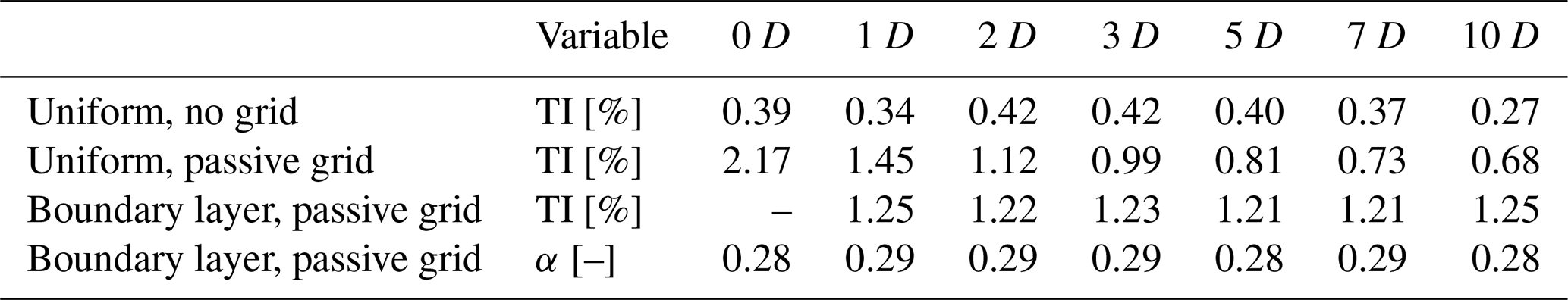
The turbulence intensity (TI) and the shear exponent (α) at hub height are determined by the WindScanner using the staring mode measurements at hub height (TI) and the averaged vertical planes (α). Each inflow condition was measured with and without the model turbine, in order to investigate the propagation of the flow field within the segments. Besides altering the inflow conditions the operational conditions of the turbine model were also modified by changing the yaw angle (ψ). The turbine was yawed at , 0, and 30∘. The turbine yaw angle is defined as positive when the turbine nacelle is rotated in the clockwise direction when looking at the turbine from above. This leads to unique measurement conditions.
For the case with no grid, the flow was measured in a horizontal plane at hub height and in vertical planes at 1, 2, 3, 5, 13, and 16 D, with and without the turbine installed. For the measurement case with the uniform passive grid and the sheared inflow, the flow is measured at 1, 2, 3, 5, 7, and 10 D, with an additional case at 0 D without a turbine. The measurements were performed plane by plane and not simultaneously. In addition to the vertical planes and the horizontal planes, staring mode measurements at a single point were also performed at 0, 1, 2, 3, 5, 7, and 10 D at hub height for a duration of 10 min to obtain data with a frequency of 451.7 Hz with and without the turbine installed. The staring mode measurements with sheared inflow an 0 D are not included due to a faulty data set.
2.3 Wake centre detection
Two different methods were used to determine the wake centre. The first method determines the wake centre by calculating the position of the minimal potential power of a virtual downstream turbine, described by Schottler et al. (2017). The potential power in the wind (P*) is determined with Eq. (3), which divides the rotor area in five ring segments. Within the area (Ai) of a ring segment, the spatially and temporally averaged velocity and the air density (ρ) are used to calculate the power. The potential power is the result of the summation of the power determined for each individual ring segment with a width of 6 cm, which is below the resolution of the interpolation grid. The location of the lowest potential power (and hence the wake centre) is obtained by computing the potential ring at hub height in the range between −1 .
The second method is performed by extracting the temporally averaged velocity deficit across a horizontal line at hub height from the vertical scan and fitting it with a single peak Gaussian at each downstream distance, similar to the method used by Fleming et al. (2014).
2.4 Energy dissipation rate estimation
The turbulent kinetic energy dissipation rate ε indicates the amount of energy lost due to the viscous forces in a turbulent flow. ε can be determined by using the raw Doppler spectrum width acquired from the WindScanner for each measurement case, in order to analyse the behaviour of the wake for different inflow and turbine operating conditions. The energy dissipation rate was determined using Eq. (4) derived by Banakh and Smalikho (1999). Here, σs is the spectrum width, C≈1.5 is the Kolmogorov constant, and l is the Rayleigh length corresponding to the filtering of the small-scale turbulence. The Rayleigh length for a continuous-wave lidar is determined with Eq. (5), where λb (=1.55 µm) is the wavelength of the laser, rb (=56mm) is the lens aperture radius, and df is the distance of the measurement point. σs is determined by fitting a Gaussian distribution over the raw spectrum. The limitation of Eq. (4) is that it can only be used when the Rayleigh length is smaller than the large-scale turbulence occurring in the flow. For the experiments reported here, the Rayleigh length ranges from l=94 mm at to l=54 mm at . Furthermore, with this expression for ε the mean velocity gradient within the probe volume is not accounted for.
Hot-wire measurements acquired by Neunaber (2019) in a similar setup and during this campaign were used to determine the one-dimensional energy dissipation rate. These measurements and the calculated dissipation rate helped to validate the measurements conducted with the WindScanner. The dissipation rate is determined with Eq. (6) for an isotropic homogeneous flow, described by Tennekes and Lumley (1972), Hinze (1975), or Monin and Yaglom (1971). Here, ν is the kinematic viscosity of the flow, σu is the variance of the flow, and λ is the Taylor micro-length scale.
The Taylor micro-length scale is determined with Eq. (7) using the energy spectrum over the wave number k (), where f is the frequency and u is the mean velocity. The term is determined by integrating the energy spectrum (Eq. 8) between the minimum wave numbers (kmin) and the large wave numbers (kmax), above where the turbulence only contains artefacts (e.g. due to the measurement system) but no flow events according to Neunaber (2019). The value for kmax can be found by identifying the local minimum from the energy spectrum. The value for kmin is determined by identifying the wavelength at which the energy spectrum corresponds to .
The results for the flow field within the empty test section at each inflow condition are presented in Sect. 3.1. Then, the effects of the inflow conditions and operational settings (yaw angle) on the wake characteristics are analysed. The temporally averaged streamwise velocity results, the turbulent kinetic energy dissipation rate, the wake shape, and the wake deflection are presented each in a subsequent section.
3.1 Undisturbed flow propagation through the test section
To conduct a meaningful analysis of wake characteristics a well-defined flow field is required. It is preferred that the turbulence and wind shear characteristics do not significantly change within the measurement domain. This was verified by measuring the flow in the empty test section for all three inflow conditions. The measurements were analysed by spatially averaging the mean streamwise velocity component at each height (z) for all values of horizontal position (y) between −1.5 . The mean flow between 1 and 16 D for the case without grid is presented in Fig. 2a. The mean flow between 0 and 10 D for the cases with a uniform passive grid and the sheared (boundary layer) inflow is given in Fig. 2b and c, respectively.
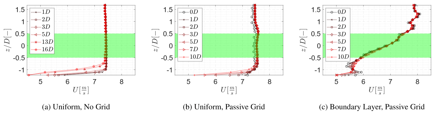
Figure 2Mean velocity U [m s−1] spatially averaged at each height position z for all values of y between , extracted from the measurements within vertical planes at multiple downstream positions. Green: rotor area.
The uniformity of the flow for the inflow condition without grid (Fig. 2a) confirms the stability of the flow throughout the measurement domain. Furthermore, the boundary layer developing on the wind tunnel floor appears unlikely to influence turbine wake development, as it is grows from at 1 D to at 16 D, which remains well below the rotor area (highlighted as a shaded green area). Analysis of the mean wake flow at 13 and 16 D indicated a minor influence of the boundary layer on the wake shape.
The mean flow for the case with a uniform passive grid also indicates a stable condition (Fig. 2b). A similar growth of the boundary layer, from at 1 D to at 10 D, is observed (Fig. 2c). The boundary layer appears to grow slightly faster than for the case without grid due to the increase in the turbulence intensity which raises mixing between the boundary layer and the steady flow. A small speed-up of 1.3 % between 0 and 1 D is visible, due to the decay of the turbulent structures. It is assumed that this has a minor effect on the wake behaviour as the inflow condition remained stable with no speed-up from 1 up to 10 D.
The mean flow for the case of the passive grid with variable open area does not show a well-behaved boundary layer close to the wall (Fig. 2c), due to a slight speed-up of the mean wind speed between . A possible cause of the speed-up is the distribution of the blockage over the inlet area. Due to the positioning of the first flap, the blockage between the wind tunnel segment floor and the first row of flaps is lower in comparison to the blockage between the first and second row of flaps. However, the flow field within the rotor area showed a near-constant shear exponent (power law fitted over the vertical extent of the rotor area), with a variation between α=0.28 and α=0.27 within the rotor area. The slight variation is considered to have a negligible effect on the wake characteristics. This indicates that flow is stable and provides a reasonable approximation of an atmospheric boundary layer flow and is suitable for the investigation of turbine wake characteristics.
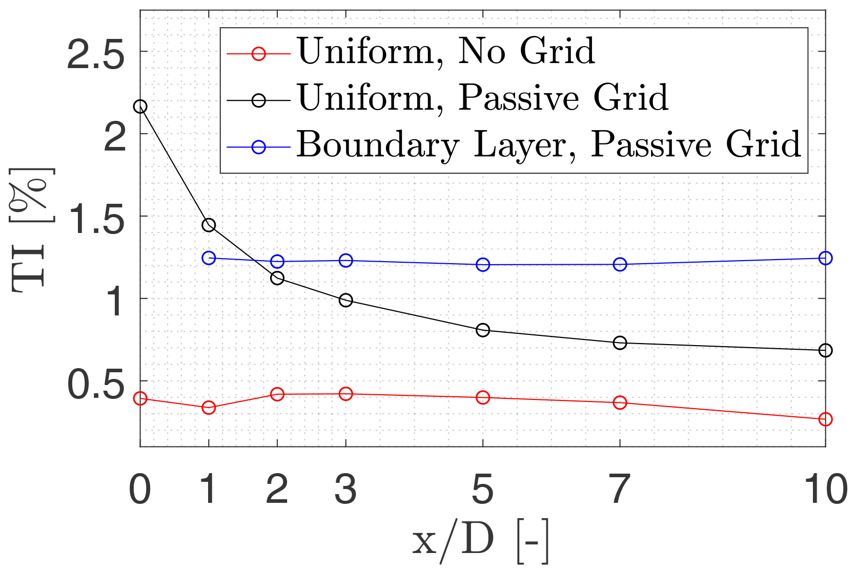
Figure 3Turbulence intensity for each inflow condition within the wind tunnel segments at each downstream distance at hub height conducted with the staring mode measurements. Note that in the turbine coordinate system is 2.4 D downstream of the inlet/grid.
In addition to the mean flow, turbulence characteristics are crucial to determine the stability of the flow. The analysis was conducted using the staring mode measurements at hub height at the centre of the wind tunnel, shown in Fig. 3. As expected, the turbulence intensity remains approximately constant around 0.37 % for the case without grid (empty nozzle). For the inflow condition with a uniform passive grid, the turbulence is higher initially, and it rapidly decays moving downstream and stabilises after 5 D. Groth and Johansson (1988) indicated that the turbulence length scale decays behind a passive grid and thus leads to the reduction of the turbulence intensity. The effect of the turbulence decay on the wake characteristics is considered to be minor as the turbulence intensity reduces from 1.5 % to 0.7 % between 1 and 10 D. For the inflow condition with the variable-open-area grid (boundary layer), the turbulence intensity remains approximately constant around 1.3 % after 1 . This suggests that turbulence is maintained at a near-constant level due to the mean shear, which causes production of turbulent kinetic energy between . The variable open area reduces the generated turbulence length scale at the grid and thus leads to a faster decay of the turbulence intensity in the region between the grid and 1 .
3.2 Wake characteristics at different operational and inflow conditions
Through the use of multiple scanning planes with the WindScanner, the evolution of the wake can be analysed in detail for each inflow condition. As representative locations, the measurements at 2 and 5 D will be compared for the nine combinations of inflow and turbine operating conditions. In the case of turbulent inflow, the tip and root vortices start to break down at 2 D, whereas they have broken down by 4 D (Neunaber et al., 2020) in the case with no grid, and the wake is transitioning out of its near-wake character. By 5 D the wake has achieved far-wake character (as defined for wind turbines), while still exhibiting a pronounced wake signature.
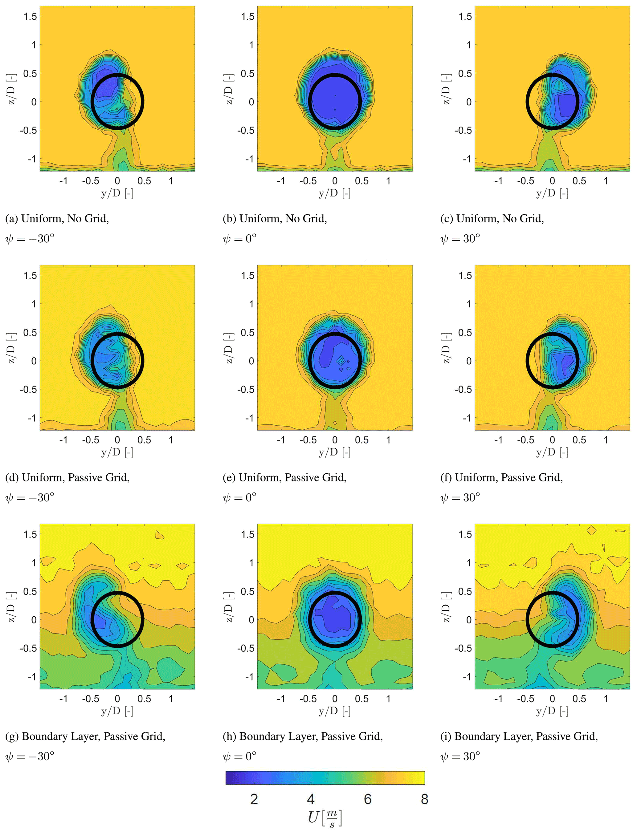
Figure 4Temporally averaged streamwise velocity component at a downstream distance of 2 D for different inflow conditions. The wake is viewed looking upstream towards the turbine model.
Figure 4 shows the wake characteristics at 2 D downstream from the turbine for each inflow condition and for the yaw angles of , 0, and 30∘. This figure highlights the symmetric behaviour, at ψ=0∘, and the asymmetric behaviour of the wake, at ∘. The development of the curled wake due to the CVP described by Bastankhah and Porté-Agel (2016) is visible. The curled wake is visible for the case with a boundary layer inflow, while the wake is no longer axisymmetric for the cases with uniform inflow.
Next to the development of the curled wake, the wake of the tower is also visible in Fig. 4. Here, it can be detected that the tower wake experiences a lateral displacement in the opposite direction of the wake deflection, with no lateral movement for the case of ψ=0∘. This is a result of conservation of mass, balancing the lateral velocity component at hub height created by the CVP with a lateral momentum in the opposite direction at a large yaw angle. This may be an effect of conducting the experiment in a closed test section and should be investigated further.
Figure 4a and c indicate an asymmetric distribution of the wind speed within the wake. For a yaw angle of ∘ (Fig. 4a), the upper part of the wake area has a lower wind speed in comparison to the lower part of the wake. Due to the large yaw angle and the clockwise rotation of the turbine, the blades of the turbine will either rotate into or with the wind, thus changing the relative wind speed and the angle of attack. In the case with ∘ (Fig. 4a), the blades turn into the wind in the upper part of the rotor area, increasing the relative wind speed.
The opposite occurs with ψ=30∘ (Fig. 4c). In addition, the difference between the wind speed deficit in the upper part and the lower part seems to be reduced for the case with a uniform passive grid shown in Fig. 4d to f. Both cases were conducted with a uniform inflow condition and the same wind speed, which indicates that the distribution of the momentum deficit behind the rotor should be equal. This suggests that the difference is related to the higher turbulence intensity and the higher mixing rate. Figure 4g to i indicate that the lowest wind speed region is approximately at hub height.
At 2 D with ∘ (Fig. 4g) the region with the lowest wind speed propagates to the lower part of the wake area. The opposite occurs at ψ=30∘ (Fig. 4i). In addition, it is also visible that the shear layer of the wake with the surrounding flow is less severe in comparison to the other inflow cases, due to the higher turbulence intensity.
Figure 5 presents the wake characteristics at 5 D downstream from the turbine for each inflow condition and for the yaw angles of , 0, and 30∘, 3 D further downstream than Fig. 4. At this distance the wake has evolved to a curled wake shape for each inflow condition for ∘, indicating that the lateral displacement induced by the CVP increased further downstream.
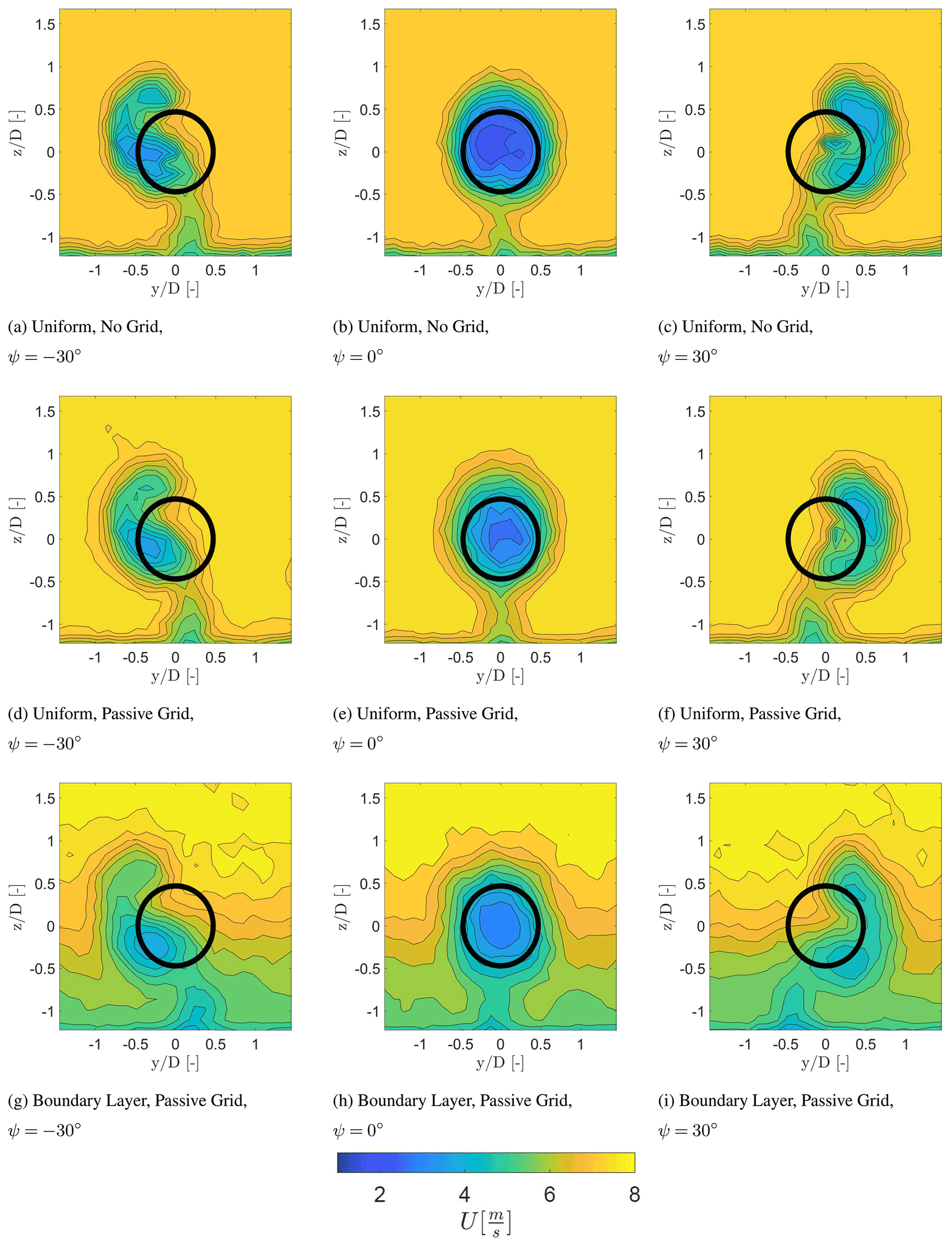
Figure 5Temporally averaged streamwise velocity component at a downstream distance of 5 D for different inflow conditions. The wake is viewed looking upstream towards the turbine model.
This is consistent with the findings of Bastankhah and Porté-Agel (2016). In addition, with the increased lateral displacement of the turbine wake at hub height, the wake of the tower also experienced a larger lateral displacement in the opposite direction for the cases with ∘, as expected. Furthermore, the wake experiences mixing between the boundary of the wake and the ambient flow (Sanderse, 2009). Here, it can be seen that the mixing layer between the wake and the free-stream velocity is smaller at the inflow condition with no grid in comparison to the inflow condition with a passive grid and a boundary layer. This effect is due to the higher turbulence intensity in the latter two cases. As expected the wake mixing layer grows for all cases as the wake evolves downstream.
The region with the highest wake deficit is pushed to a certain direction depending on the yaw angle, highlighted in Fig. 6. The movement is due to the combination of the wake rotation and the CVP described in Martínez-Tossas et al. (2019). The comparison between Figs. 4 and 5 indicates that the wake deficit transferred to the lower part of the wake area for ∘ and to the upper part for ψ=30∘ for each inflow case. The advection of the wake deficit is visualised in Fig. 6 for each inflow case at each downstream distance. The centre is determined with the normalised local velocity () by calculating the centroid over the region below the threshold , uthresh=0.25 m s−1. Figure 6 illustrates that the deficit is transferred with the counterclockwise rotation of the wake when looking downstream. This has also been described in Bastankhah and Porté-Agel (2016), showing the displacement of the wake centre predicted by the potential flow theory. It should be noted that there is some scatter in Fig. 6a for the position of the wake deficit at 13 D and at 16 D, since the wake velocity deficit has further decayed, which makes the wake centre detection methods less accurate for the given measurement resolution.
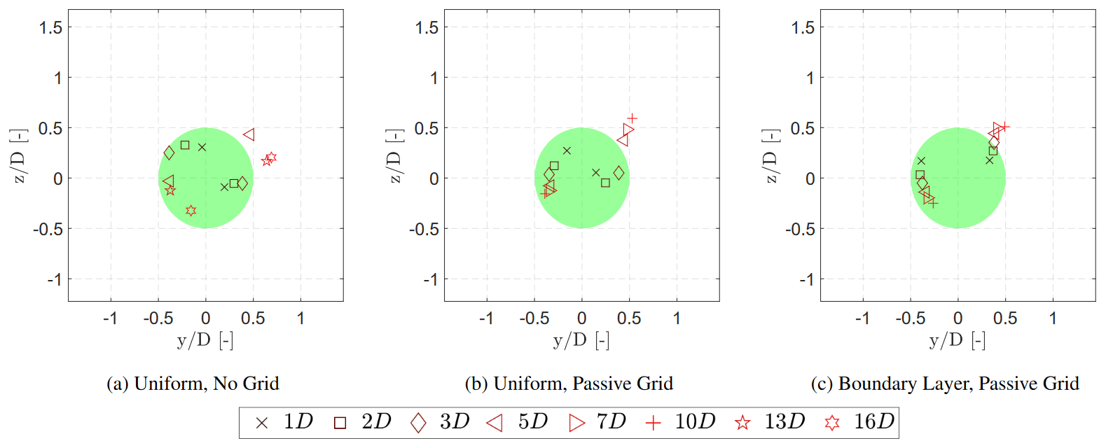
Figure 6Location of the largest mean velocity deficit normalised over the local velocity () for each inflow condition at each downstream position for ∘. At ∘ the positions are located at y<0. At ψ=30∘ the positions are located at y>0.
3.3 Evolution of the energy dissipation rate
The turbulent kinetic energy dissipation rate (ε) is typically increased for increased turbulent mixing within a wake. Increased turbulent mixing leads to faster wake recovery, and, thus, the dissipation rate can be seen as an indirect indicator of how the flow will evolve within the wake: a high dissipation rate suggests more mixing of the wake, whereas a small dissipation rate suggests less mixing and that the wake will persist further downstream. Figure 7 indicates the estimated ε (Eq. 4) of the wake at a downstream distance of 2 D. The first noticeable difference is that the energy dissipation rate is slightly lower in the case with no grid (Fig. 7a to c) in comparison to the situations with a passive grid or a boundary layer, as expected. This is related to the higher turbulence in the inflow in the latter two conditions.
Moreover, an increased dissipation rate was detected within the wake in comparison to the ambient flow, which corresponds to Lundquist and Bariteau (2015). For ψ=0∘, a ring-shaped area of increased dissipation slightly larger than the rotor area exists for each inflow condition, which overlaps with the wake mixing layer and is consistent with the findings of Eriksen and Krogstad (2017), Bartl and Sætran (2017), and Schottler et al. (2018). A similar behaviour is seen with the wake generated by the tower. Moreover, the energy dissipation rate captured within the tower wake reduces with a sheared inflow. The slightly higher dissipation rate at the wake centre visible in Fig. 7b and e in the different colour shading at the centre can be related to the root vortices within the near wake. At ∘ the circular shape of the energy dissipation is deflected to an elliptical shape with a uniform inflow or a curled shape with a sheared inflow. A region with a low dissipation rate is visible within the wake area in the case with no grid, a passive grid, and a boundary layer, corresponding to the region with the highest wake deficit, which also has comparatively lower velocity gradients. An increased energy dissipation rate is also visible in the upper part of the wake with a sheared inflow (Fig. 7g to i), which is a result of the higher velocity components resulting in a higher mixing rate between the ambient flow and the wake.
At 5 D (Fig. 8) the energy dissipation rate decreased due to the expansion of the mixing area between the wake and the ambient flow. The width of the ring visible at ∘ increased at 5 D, which is also related to the increased mixing at a larger downstream distance. Due to the breakdown of the root vortices in the near wake, the increment of the energy dissipation rate at hub height is not visible at a downstream distance of 5 D. A similar behaviour is noticeable at the upper part of the wake with sheared inflow condition indicating an increased energy dissipation rate in comparison to the lower part of the wake area. Due to the large yaw angle and the downstream distance, the circular shape of the energy dissipation rate has deformed to a curled shape for each inflow condition. In addition, similar to the flow at 2 D a low dissipation rate is also visible at the region with the highest wake deficit, as it is related to the gradient of Reynolds stresses. The energy dissipation is larger in the uniform inflow cases in comparison to the sheared cases at 5 D. This could be related to the increased mixing with a sheared inflow between the regions with a higher wind speed in comparison to the regions with a lower wind speed, resulting in a faster decay of the flow. This is visible in Fig. 7d–f showing a larger region with a high energy dissipation rate with a sheared inflow at 2 D in comparison to the uniform inflow cases. This indicates that the wake will break down faster in a boundary layer, whereas the wake deficit persists for a longer period of time with a uniform inflow condition.
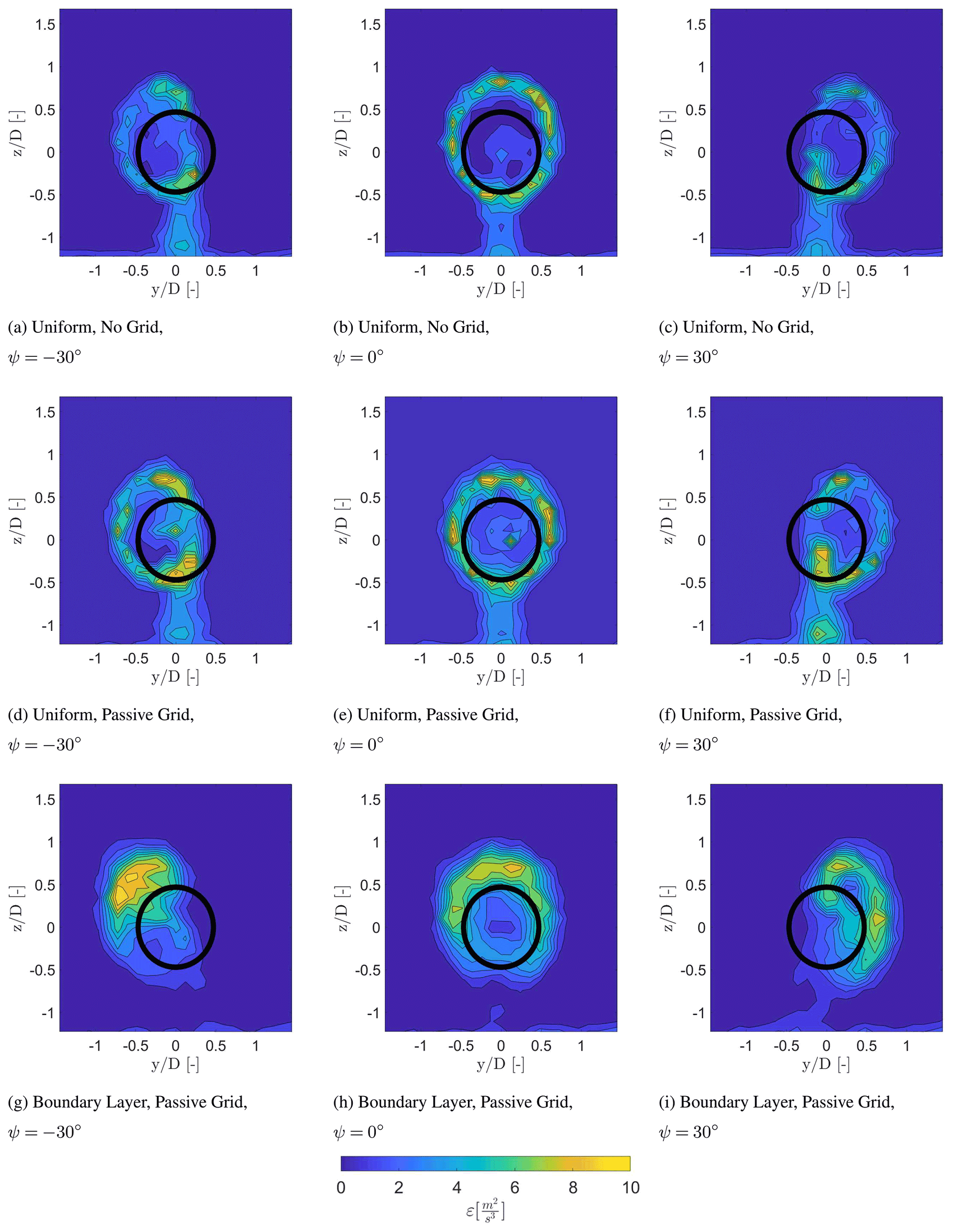
Figure 7Energy dissipation rate within the wake at a downstream distance of 2 D for different inflow conditions. The wake is viewed looking upstream towards the turbine model.
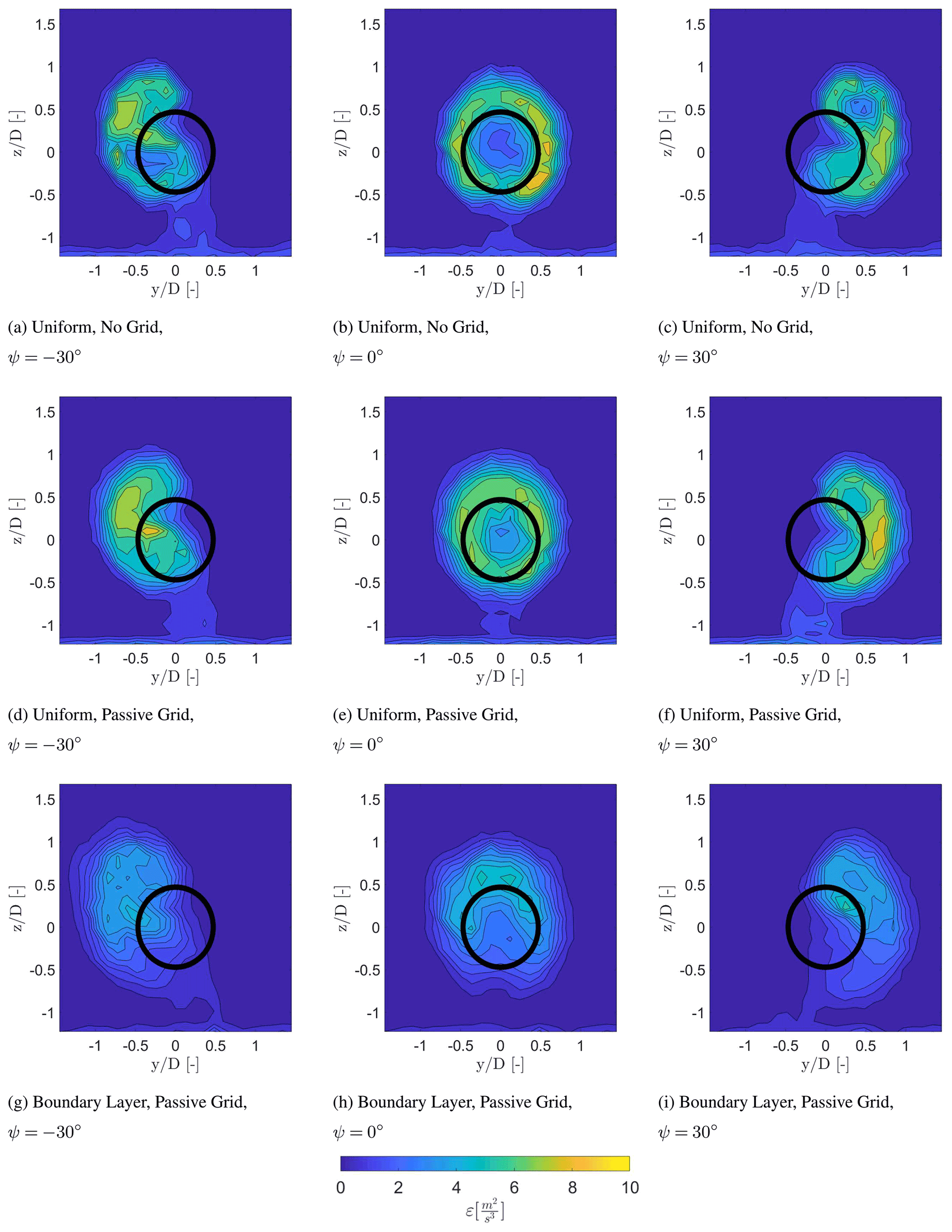
Figure 8Energy dissipation rate within the wake at a downstream distance of 5 D for different inflow conditions. The wake is viewed looking upstream towards the turbine model.
3.4 Development of the curled wake shape
Figure 9 visualises the growth of the curled wake behind the turbine. The contour lines indicate the boundary of the wake determined by implementing a threshold to the normalised local velocity with the free-stream velocity. The threshold is set at . The formation of a curled wake shape is due to the CVP as described by Bastankhah and Porté-Agel (2016), leading to a lateral velocity component at hub height and two vortex pairs, rotating in the opposite direction, at the top and bottom of the rotor area depending on the yaw angle. This was also observed by Vollmer et al. (2016) at different atmospheric conditions and was implemented in the FLORIS model by Martínez-Tossas et al. (2019).

Figure 9Growth of the curled wake behind the wind turbine model at multiple downstream distances. The contour lines indicate the boundary with at each downstream location. The view is looking upstream towards the turbine model.

Figure 10Position of the minimum velocity determined at each z position for each inflow condition. Dotted lines: uniform, passive grid. Solid lines: boundary layer, passive grid.
It can be seen in Fig. 9a and b that the wake area is no longer axisymmetric in the near-wake region. The wake then evolves to a curled shape between 3–5 D for for the inflow condition with a uniform passive grid. A similar trend is observed with the inflow condition without a grid (not shown in this paper). For the case with a boundary layer inflow (Fig. 9c and d), the wake area evolved sooner to the curled shape between 2–3 D. This can also be recognised in Fig. 10, which plots the y position of the minimum wake velocity (largest velocity deficit) for each z position. In order to determine the largest velocity deficit, the measurement data presented in Figs. 4 and 5 are smoothed to remove local fluctuations. This resulted in arc-shaped curves which provide a direct comparison of the wake shape for different inflow conditions, similar to Bartl et al. (2018). For the case with a uniform inflow an almost straight line is observed at 2 D for ∘, which slowly shapes to an arc-shaped curve at 3 D. In the case with a boundary layer inflow the curve is already arc-shaped at 1 D for ∘. This indicates that the combination of the shear layer, the wake rotation, and the CVP increases the lateral velocity at hub height induced by the CVP, thus increasing the vortex strength of the CVP in comparison to a uniform case. In addition, at ∘ the wake experiences a larger deflection of the minimum velocity with a boundary layer inflow in comparison to the case with a uniform inflow, which corresponds with the presence of a stronger CVP. Moreover, the maximum deflection of ±0.72 D is symmetric for the inflow with a uniform passive grid for ∘. For a boundary layer inflow, the maximum deflection is slightly asymmetric with 0.72 D for ψ=30∘ and −0.81 D for ∘. This is related to the combination of the counterclockwise rotation of the wake and the sheared inflow, leading to an increase or a decrease in the relative velocity and hence the vortex strength depending on the yaw angle as described in Sect. 3.2.

Figure 11Wake deflection at different inflow condition determined with the methods described by Schottler et al. (2018). The wake centre is derived from the vertical scans at each downstream distance. The shaded area indicates the spread of the wake centre determined for each individual vertical scan. Black: Gaussian method. Red: minimal potential power method.
3.5 Wake deflection at different inflow conditions
The influence of the different inflow conditions and operational conditions on the deflection of the wake is further analysed here using the methods described in Sect. 2.3. Figure 11 illustrates the wake centre for each inflow condition computed with the Gaussian function and the minimal power (Sect. 2.3). The shaded area indicates the spread (±σ) of the wake centre derived from the individual scans with both methods. The Gaussian-based method results in large wake deflections in all yawed cases, since it is influenced by the location of the largest velocity deficit at hub height, in contrast to the minimal potential power method which accounts for the overall wake area. The difference is also related to the development of the curled shape, shown in Fig. 10, illustrating an arc-shaped curve of the highest velocity deficit. The difference between the two methods for finding the wake centre can clearly be seen for the case with a boundary layer inflow and ψ=30∘, where the wake is curled the most.
The asymmetry in the wake deflection, observed by Fleming et al. (2014), Fleming et al. (2018), and Bartl et al. (2018), is evident in Fig. 11 for the case with a boundary layer inflow. Using the method by locating the minimal potential power, the wake centre experiences a larger wake deflection for ψ=30∘ in comparison to ∘. This is due to the influence of the shear on the strength of the vorticity on the CVP and corresponds with the findings shown in Fig. 10.
The velocity data acquired with the WindScanner were validated by comparing them to the hot-wire data set from Neunaber (2019), shown in Sect. 4.1. In that study the wake characteristics were determined through multiple hot wires with the same layout, wind turbine model, inflow condition, and operational condition similar to the case with no grid and ψ=0∘ in the present campaign. The comparison is followed by an uncertainty analysis of the measurement data in Sect. 4.2.
4.1 Data comparison
Neunaber (2019) used the MoWiTO 0.6 to determine the wake characteristics at multiple downstream and lateral positions through the use of hot wires. The comparison of the temporally averaged properties of the flow is assessed by performing a visual comparison of the horizontal wake development and the vertical scans at 1, 2, 3, and 5 D. The measurement data from Neunaber (2019) were measured between and and have been mirrored during the comparison. The hot-wire data are compared with the horizontal scan measured by the WindScanner, presented in Fig. 12. Here, the lines with a marker indicate the contours for wind speeds of m s−1. The wake measured with the horizontal scan by the WindScanner shows a similar development as the wake measured by Neunaber (2019) with regards to wake growth and position of the transition of the near wake to the far wake.
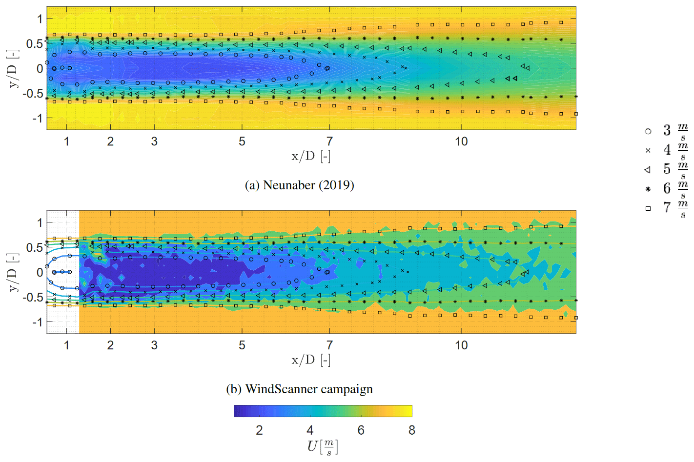
Figure 12Comparison of the profiles of the averaged streamwise velocity component at 1, 2, 3, and 5 D between the WindScanner measurements and the hot-wire measurements at Neunaber (2019). Both measurements were conducted with no grid at U=7.5 m s−1. Lines with a marker indicate the contours at m s−1.
The temporally averaged streamwise velocity component at hub height from the hot-wire measurements was compared with the vertical lidar scans at 1, 2, 3, and 5 D. At 1 D in Fig. 13 it can be seen that the wake shape obtained from the WindScanner resembles the wake deficit obtained by the hot-wire measurements. However, there is a large difference in the streamwise velocity component around . The difference can be related to the filtering process of the WindScanner, since the spectrum of the WindScanner is heavily disturbed due to the nacelle of the wind turbine resulting in a low amount of measurement samples at that grid point. At 2 to 5 D the wake profile shows a similar wake deficit and wake width. However, small differences are noticeable in the velocity. This can also be related to the filtering process and the effect of the sampling onto the grid. Furthermore, the probe volume length is 20 cm at 1 D and 13 cm at 5 D, which also influences the measurement data. These differences can also be attributed to the location of the staring mode measurements in relation to the position of the turbine, as a small deviation can lead to a large difference, and the much larger sampling and averaging volume of the WindScanner measurements, which can cause spatial averaging of the turbulence. The difference in the sampling frequency and the spatial averaging by the probe volume also affects the temporally averaged properties of the flow.
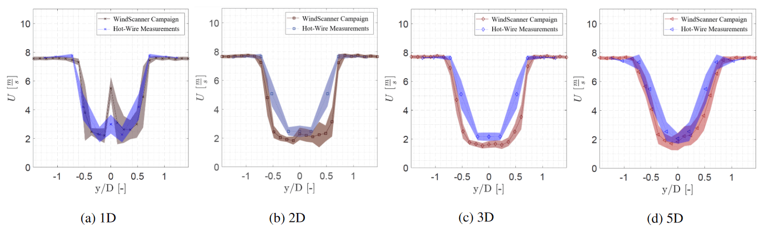
Figure 13Comparison of the profiles of the averaged streamwise velocity component at 1, 2, 3, and 5 D between the WindScanner measurements and the hot-wire measurements at Neunaber (2019). Both measurements were conducted with no grid at U=7.5 m s−1. The shaded area shows the ±σ of the measurement data.
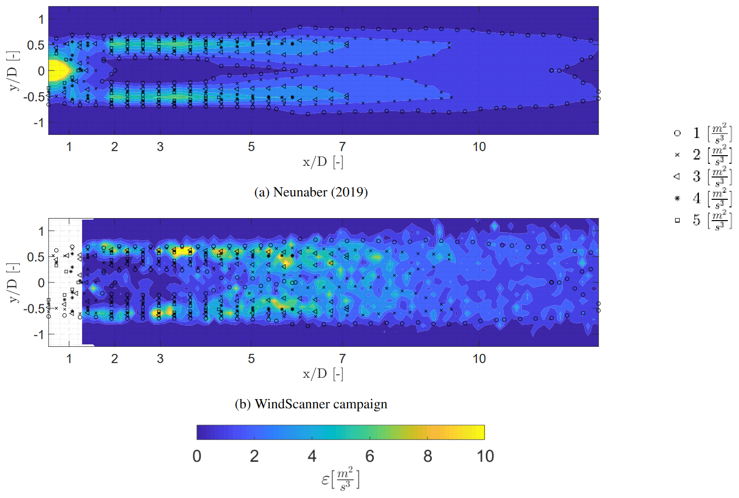
The energy dissipation rate acquired from the staring mode measurements with the WindScanner was compared to the energy dissipation rates measured with the hot wires at 10 D behind the turbine. This resulted in energy dissipation rates of and respectively.
Figure 14 indicates that the development of the energy dissipation rate within the wake is similar in comparison to the data obtained by Neunaber (2019), showing a low energy dissipation rate within the near-wake region and outside of the wake. The dissipation rate reaches its highest value near the edges of the wake in regions of high shear. This indicates a radial dependency of the energy dissipation rate within the wake, also suggested in Neunaber et al. (2021). Further downstream the energy dissipation rate slowly reduces. The reduction agrees with Figs. 7b and 8b, showing a ring with a high energy dissipation rate slightly larger than the rotor area which increases in width at downstream location of 5 D . Furthermore, the energy dissipation at the rotor centre increases up to 5–7 D, after which it reduces. This also agrees with Figs. 7b and 8b, showing an increase in the energy dissipation rate at the rotor centre.
The comparison of the energy dissipation rates between the two measurement techniques is further expanded in Fig. 15, showing the energy dissipation rate at hub height. A similar trend is visible, showing a high energy dissipation rate at at 1 D and at the shear layer between the wake and the free-stream flow at 2 to 5 D. Moreover the energy dissipation rate obtained from the WindScanner is lower at 1 D in comparison to the hot-wire measurements, which could be due to the backscatter of the blades affecting the measurements.
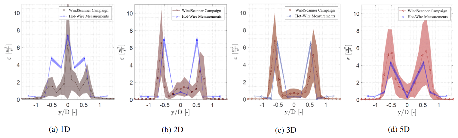
However, at 2 to 5 D it is noticeable that the magnitude of the energy dissipation rate obtained with the WindScanner differs in comparison to the hot-wire measurements. This can be attributed to the probe volume crossing the entire wake and the difference in sampling frequency. The difference of the mean velocity gradient is not accounted for with the method used to determine the energy dissipation. Another influence is the sampling frequency and the method used to calculate the energy dissipation rate from the hot-wire measurements, where the energy spectrum has been cut off at a certain wave number to exclude artefacts in the turbulence.
In addition, the measurements obtained with the hot wires during the WindScanner campaign indicate a similar magnitude of the streamwise velocity and energy dissipation rate with the WindScanner measurements shown in Fig. 16. The temporal averaged velocity, shown in Fig. 5i, indicates a similar curvature of the wake (red crosses) in comparison to the WindScanner data (blue crosses). Similar to the WindScanner data (Fig. 8i), a higher dissipation rate is also observed with the hot-wire measurements (Fig. 16b) at the upper region of the wake () in comparison to the lower region (). Moreover, within the ambient air, an energy dissipation rate of is observed, which corresponds to the measurements with the WindScanner. The energy dissipation rate has a similar magnitude as the one obtained with the WindScanner in the upper region of the wake, while in the lower region of the wake a difference is noticeable. The difference can be due to the probe volume averaging of the WindScanner, as the volume (13 cm at 5 D) crosses the entire wake, leading to unwanted artefacts in the spectrum. This indicates that the WindScanner is able to capture the main trends of the development of the energy dissipation rate but that it is affected due to the probe volume averaging.

Figure 16Temporal averaged velocity (a) and energy dissipation rate (b) obtained from the hot-wire measurements conducted in the WindScanner campaign. The position of the minimum velocity determined at each z position, which indicates the curvature of the wake centre, obtained from the WindScanner (blue crosses) and the hot wire (red crosses) is visualised.
4.2 Uncertainty analysis
The uncertainty analysis for the estimation of the u component is conducted following the standard uncertainty method performed by Stawiarski et al. (2013) and van Dooren et al. (2016). The investigation was conducted by considering the uncertainty of the lidar measurement and the reconstruction for the streamwise velocity component at a downstream distance of 2 and 5 D, computed using Eq. (2), to determine the uncertainties of the horizontal velocity component eu. In Eq. (9), ev and ew are the uncertainty of the u and w component, eδ and eθ are the uncertainty of the azimuth and elevation angle, and evlos is the uncertainty of the measured line-of-sight velocity. evlos is assumed to be 1 % according to Pedersen et al. (2012). In addition, the maximum uncertainty of the w and v component is set to be 1 m s−1 at 1, 5, and 10 D. This is due to the strong vortices within the near wake. Furthermore, the pointing error is assumed to be 0.05 mrad for the elevation and the azimuth angle (van Dooren et al., 2017).
Figure 17 presents the error obtained with Eq. (9) for the cases 2 and 5 D for the inflow condition without a grid normalised with the horizontal velocity component at a certain position ( [%]). At a downstream distance of 2 D, the error is between 1 % in the ambient air and 3.1 % within the wake. This is expected since the line-of-sight velocity is lower within the wake. In addition, the error is larger at the upper part of the measurement domain () in comparison to the lower region (), due to the larger elevation angle of the laser beam. This leads to an error of 1.5 % in the upper region and 1 % in the lower region at 2 and 5 D. Within the wake the error ranges between 3.1 % and 2.6 % at 2 and 5 D respectively. During misaligned cases the assumption v≈0 and w≈0 does not hold. At an uncertainty of 1 m s−1 for the w and v component an uncertainty ranging from 2.1 % to 1.6 % within the wake at 2 and 5 D is observed.

Additionally, the statistical uncertainty needs to be considered using the margin of error , where N is the sample size, σ is the standard deviation of the measurements, and zγ is the quantile set to 1.96 which equals to a 95 % confidence interval. Figure 18 shows the margin of error of the streamwise velocity component for each grid point at a downstream distance of 2 and 5 D. The margin of error is higher in the wake in comparison to the ambient air due to the simple fact of a higher standard deviation of the streamwise velocity component. The margin of error is around 0.3 m s−1 at 2 D and around 0.15 m s−1 at 5 D.
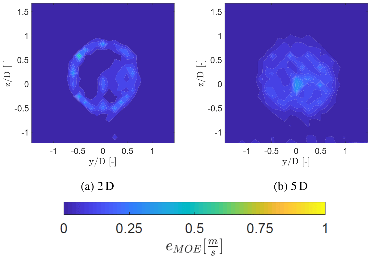
Figure 18Margin of error (eMOE) of the streamwise velocity at 2 and 5 D for the inflow without a grid.
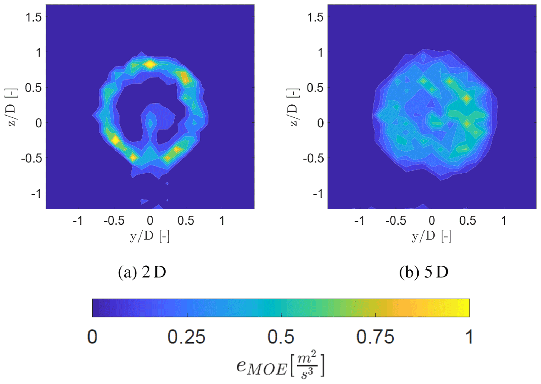
Figure 19Margin of error (eMOE) of the energy dissipation rate at 2 and 5 D for the inflow without a grid.
At some locations a high margin of error is visible due to a low amount of measurement data, caused by the filtering process and the Lissajous pattern resulting in a reduced amount of data at and . The margin of error of the energy dissipation rate is shown in Fig. 19, indicating a similar trend visible in Fig. 18. Here the margin of error is around 0.6 m2 s−3 at 2 D and around 0.4 m2 s−3 at 5 D. The margin of error has a larger magnitude as the width of the spectrum is squared in Eq. (4). This also explains the larger scatter in the dissipation rate contours of Figs. 7 and 8, compared to the mean velocity contours of Figs. 4 and 5. This indicates that the WindScanner is able to capture the averaged flow properties such as the streamwise velocity and the main trends of the development of the energy dissipation rate.
In general, a strong dependency of the wake characteristics on both the yaw angle and the inflow conditions was observed. Three different inflow conditions were generated: one without a grid, one with a uniform-open-area passive grid, and one with a variable-open-area passive grid which created an inflow with mean shear approximating a boundary layer. The wakes of a model wind turbine (MoWiTO 0.6) were measured with turbines operating at maximum power coefficient at a flow speed of 7.5 m s−1 for rotor yaw angles of 0, +30, and −30∘, and the empty test section flow was measured as well.
Measurements of the free-stream flow within the test section with the noninvasive short-range lidar WindScanner indicated a stable flow for each inflow condition and no large influence of the boundary layer due to the wind tunnel wall on the wake. For the cases with yaw ∘, the wake was deflected laterally up to 0.6 D, and a curled wake was observed. The curled wake develops sooner and is stronger in the case of the boundary layer inflow compared to the uniform inflow, suggesting that boundary layer inflow increases the counter-rotating vortex pair (CVP). The wake deficit distribution in these cases is asymmetric due to the rotation of the turbine and the yaw angle changing the relative wind speed across the rotor plane. The tower wake was observed to be displaced in the opposite direction of the deflection of the turbine wake. The presence of a stronger CVP leads to an asymmetry in the wake deflection with a boundary layer, in contrast to the cases with a uniform inflow condition.
The analyses of the energy dissipation rate showed a higher energy dissipation rate within the wake in comparison to the ambient flow. A lower magnitude of the energy dissipation rate is identified at a lower turbulence. In addition, a ring with increased energy dissipation slightly larger than the rotor area and growing in width further downstream is visible for each inflow condition. At ±30∘ yaw the circular shape is stretched to an axisymmetric shape or a curled shaped, depending on the inflow condition and the downstream distance.
The WindScanner measurements showed a good comparison with the hot-wire data obtained by Neunaber (2019) and the current campaign. However, the WindScanner partially filters out the turbulence due to the Lorentzian spatial weighting function of the measurement device. A similar trend of the temporal averaged streamwise velocity component and the energy dissipation is observed between each data set. However, differences in the magnitude of the temporal averaged streamwise velocity component and the energy dissipation were observed, which is related to the filtering process, the sampling frequency, the probe volume, and the method used to determine the energy dissipation from the hot-wire data and the WindScanner. Additionally, an uncertainty analysis indicated a relative error of the measurement data up to 3.5 % and a margin of error of around 0.3 m s−1 at 2 D and 0.15 m s−1 at 5 D for the streamwise velocity component. The measurements of the energy dissipation showed a margin of error around 0.6 m2 s−3 at 2 D and 0.4 m2 s−3 at 5 D.
Due to the possibility of mapping the wake fast at multiple locations with the WindScanner, a thorough understanding of the development of the wake is acquired at different inflow conditions and operational conditions. This will aid the process to further improve existing wake models by accounting for the near wake and the dissipation of the wake. Future steps are to compare the acquired data with numerical simulation with the same inflow condition and existing wake models.
The data presented here are published at https://doi.org/10.5281/zenodo.5734877 (Hulsman et al., 2021).
PH designed the research, conducted the measurement campaign, performed the data analysis, prepared the figures, and planned and wrote the paper. MW contributed to the wind tunnel campaign, data analysis, and writing of the paper. MH contributed on the operation of the wind tunnel, the active grid, and the model wind turbine. MK supervised the work. VP helped with designing the research, the data analysis, and the writing of the paper. All co-authors contributed with several fruitful discussions and thoroughly reviewed the manuscript.
The contact author has declared that neither they nor their co-authors have any competing interests.
Publisher's note: Copernicus Publications remains neutral with regard to jurisdictional claims in published maps and institutional affiliations.
The authors would like to thank Ingrid Neunaber for providing the hot-wire data which were obtained during her PhD, funded by the German Federal Environmental Foundation, DBU (no. 20014/342). Furthermore, we would like to thank our colleagues Marijn Floris van Dooren and Anantha Padmanabhan Kidambi Sekar for their assistance during the extensive WindScanner measurement campaign.
This work is partly funded by the Federal Ministry for Economic Affairs and Energy according to a resolution by the German federal parliament in the scope of research project CompactWind II (ref. no. 0325492H) and DFWind (ref. no. 0325936C). Martin Wosnik received support by the Hanse-Wissenschaftskolleg (HWK) Institute for Advanced Study, where he was a fellow while this work was carried out.
This paper was edited by Johan Meyers and reviewed by two anonymous referees.
Banakh, V. A. and Smalikho, I. N.: Measurements of Turbulent Energy Dissipation Rate with a CW Doppler Lidar in the Atmospheric Boundary Layer, J. Atmos. Ocean. Tech., 16, 1044–1061, https://doi.org/10.1175/1520-0426(1999)016<1044:MOTEDR>2.0.CO;2, 1999. a
Barthelmie, R. J., Pryor, S. C., Frandsen, S. T., Hansen, K. S., Schepers, J., Rados, K., Schlez, W., Neubert, A., Jensen, L., and Neckelmann, S.: Quantifying the impact of wind turbine wakes on power output at offshore wind farms, J. Atmos. Ocean. Tech., 27, 1302–1317, https://doi.org/10.1175/2010JTECHA1398.1, 2010. a
Bartl, J. and Sætran, L.: Blind test comparison of the performance and wake flow between two in-line wind turbines exposed to different turbulent inflow conditions, Wind Energ. Sci., 2, 55–76, https://doi.org/10.5194/wes-2-55-2017, 2017. a
Bartl, J., Mühle, F., Schottler, J., Sætran, L., Peinke, J., Adaramola, M., and Hölling, M.: Wind tunnel experiments on wind turbine wakes in yaw: effects of inflow turbulence and shear, Wind Energ. Sci., 3, 329–343, https://doi.org/10.5194/wes-3-329-2018, 2018. a, b, c, d
Bastankhah, M. and Porté-Agel, F.: Experimental and theoretical study of wind turbine wakes in yawed conditions, J. Fluid Mech., 806, 506–541, https://doi.org/10.1017/jfm.2016.595, 2016. a, b, c, d, e, f, g
Eriksen, P. E. and Krogstad, P.-Å.: Development of coherent motion in the wake of a model wind turbine, Renew. Energ., 108, 449–460, https://doi.org/10.1016/j.renene.2017.02.031, 2017. a
Fleming, P., Annoni, J., Churchfield, M., Martinez-Tossas, L. A., Gruchalla, K., Lawson, M., and Moriarty, P.: A simulation study demonstrating the importance of large-scale trailing vortices in wake steering, Wind Energ. Sci., 3, 243–255, https://doi.org/10.5194/wes-3-243-2018, 2018. a
Fleming, P., King, J., Dykes, K., Simley, E., Roadman, J., Scholbrock, A., Murphy, P., Lundquist, J. K., Moriarty, P., Fleming, K., van Dam, J., Bay, C., Mudafort, R., Lopez, H., Skopek, J., Scott, M., Ryan, B., Guernsey, C., and Brake, D.: Initial results from a field campaign of wake steering applied at a commercial wind farm – Part 1, Wind Energ. Sci., 4, 273–285, https://doi.org/10.5194/wes-4-273-2019, 2019. a
Fleming, P. A., Gebraad, P. M., Lee, S., van Wingerden, J.-W., Johnson, K., Churchfield, M., Michalakes, J., Spalart, P., and Moriarty, P.: Evaluating techniques for redirecting turbine wakes using SOWFA, Renew. Energ., 70, 211–218, https://doi.org/10.1016/j.renene.2014.02.015, 2014. a, b, c
Gebraad, P., Thomas, J. J., Ning, A., Fleming, P., and Dykes, K.: Maximization of the annual energy production of wind power plants by optimization of layout and yaw-based wake control, Wind Energy, 20, 97–107, https://doi.org/10.1002/we.1993, 2017. a
Grant, I. and Parkin, P.: A DPIV study of the trailing vortex elements from the blades of a horizontal axis wind turbine in yaw, Exp. Fluids, 28, 368–376, https://doi.org/10.1007/s003480050396, 2000. a
Grant, I., Parkin, P., and Wang, X.: Optical vortex tracking studies of a horizontal axis wind turbine in yaw using laser-sheet, flow visualisation, Exp. Fluids, 23, 513–519, https://doi.org/10.1007/s003480050142, 1997. a
Groth, J. and Johansson, A. V.: Turbulence reduction by screens, J. Fluid Mech., 197, 139–155, https://doi.org/10.1017/S0022112088003209, 1988. a
Haans, W., Sant, T., van Kuik, G., and van Bussel, G.: Measurement of tip vortex paths in the wake of a HAWT under yawed flow conditions, J. Solar Energ. Eng., 127, 456–463, https://doi.org/10.1115/1.2037092, 2005. a
Heißelmann, H., Peinke, J., and Hölling, M.: Experimental airfoil characterization under tailored turbulent conditions, J. Phys. Conf. Ser., 753, 072020, https://doi.org/10.1088/1742-6596/753/7/072020, 2016. a
Hinze, J.: Turbulence, McGraw-Hill classic textbook reissue series, McGraw-Hill, ISBN 9780070290372, 1975. a
Hulsman, P., Wosnik, M., Petrović, V., Hölling, M., and Kühn, M.: Turbine Wake Deflection Measurement in a Wind Tunnel with a Lidar WindScanner, J. Phys. Conf. Ser., 1452, 012007, https://doi.org/10.1088/1742-6596/1452/1/012007, 2020. a
Hulsman, P., Wosnik, M., Petrović, V., Hölling, M., and Kühn, M.: Data Supplement for `Curled Wake Development of a Yawed Wind Turbine at Turbulent and Sheared Inflow' – Wind Energy Science Journal, Zenodo [data set], https://doi.org/10.5281/zenodo.5734877, 2021. a
Lundquist, J. and Bariteau, L.: Dissipation of Turbulence in the Wake of a Wind Turbine, Bound.-Lay. Meteorol., 154, 229–241, https://doi.org/10.1007/s10546-014-9978-3, 2015. a, b
Martínez-Tossas, L. A., Annoni, J., Fleming, P. A., and Churchfield, M. J.: The aerodynamics of the curled wake: a simplified model in view of flow control, Wind Energ. Sci., 4, 127–138, https://doi.org/10.5194/wes-4-127-2019, 2019. a, b
Medici, D. and Alfredsson, P.: Measurements on a wind turbine wake: 3D effects and bluff body vortex shedding, Wind Energy, 9, 219–236, https://doi.org/10.1002/we.156, 2006. a, b
Monin, A. and Yaglom, A.: Statistical Fluid Mechanics: Mechanics of Turbulence, vol. 2, MIT Press, ISBN 978-0486789248, 1971. a
Neunaber, I.: Stochastic investigation of the evolution of small-scale turbulence in the wake of a wind turbine exposed to different inflow conditions, PhD thesis, University of Oldenburg, available at: http://oops.uni-oldenburg.de/3852 (last access: 14 June 2021), 2019. a, b, c, d, e, f, g, h, i, j, k, l, m, n, o
Neunaber, I., Hölling, M., Stevens, R. J., Schepers, G., and Peinke, J.: Distinct turbulent regions in the wake of a wind turbine and their inflow-dependent locations: the creation of a wake map, Energies, 13, 5392, https://doi.org/10.3390/en13205392, 2020. a, b
Neunaber, I., Peinke, J., and Obligado, M.: Investigation of the dissipation in the wake of a wind turbine array, Wind Energ. Sci. Discuss. [preprint], https://doi.org/10.5194/wes-2021-13, in review, 2021. a
Pedersen, A. T., Montes, B. F., Pedersen, J. E., Harris, M., and Mikkelsen, T.: Demonstration of short-range wind lidar in a high-performance wind tunnel, Proceedings of EWEA 2012, 2012. a
Petrović, V., Schottler, J., Neunaber, I., Hölling, M., and Kühn, M.: Wind tunnel validation of a closed loop active power control for wind farms, J. Phys. Conf. Ser., 1037, 032020, https://doi.org/10.1088/1742-6596/1037/3/032020, 2018. a
Sanderse, B.: Aerodynamics of wind turbine wakes, Energy Research Center of the Netherlands (ECN), ECN-E–09-016, Petten, the Netherlands, Tech. Rep., 5, 153, 2009. a
Schottler, J., Hölling, A., Peinke, J., and Hölling, M.: Wind tunnel tests on controllable model wind turbines in yaw, AIAA, 1523, https://doi.org/10.2514/6.2016-1523, 2016. a, b
Schottler, J., Mühle, F., Bartl, J., Peinke, J., Adaramola, M. S., Sætran, L., and Hölling, M.: Comparative study on the wake deflection behind yawed wind turbine models, J. Phys. Conf. Ser., 854, 012032, https://doi.org/10.1088/1742-6596/854/1/012032, 2017. a
Schottler, J., Bartl, J., Mühle, F., Sætran, L., Peinke, J., and Hölling, M.: Wind tunnel experiments on wind turbine wakes in yaw: redefining the wake width, Wind Energ. Sci., 3, 257–273, https://doi.org/10.5194/wes-3-257-2018, 2018. a, b, c, d
Stawiarski, C., Träumner, K., Knigge, C., and Calhoun, R.: Scopes and challenges of dual-Doppler lidar wind measurements – an error analysis, J. Atmos. Ocean. Tech., 30, 2044–2062, https://doi.org/10.1175/JTECH-D-12-00244.1, 2013. a
Tennekes, H. and Lumley, J. L.: A first course in turbulence, MIT press, ISBN 9780262200196, 1972. a
Thomsen, K. and Sørensen, P.: Fatigue loads for wind turbines operating in wakes, J. Wind Eng. Ind. Aerod., 80, 121–136, https://doi.org/10.1016/S0167-6105(98)00194-9, 1999. a
van Dooren, M., Trabucchi, D., and Kühn, M.: A methodology for the reconstruction of 2d horizontal wind fields of wind turbine wakes based on dual-Doppler lidar measurements, Remote Sensing, 8, 809, https://doi.org/10.3390/rs8100809, 2016. a
van Dooren, M. F., Campagnolo, F., Sjöholm, M., Angelou, N., Mikkelsen, T., and Kühn, M.: Demonstration and uncertainty analysis of synchronised scanning lidar measurements of 2-D velocity fields in a boundary-layer wind tunnel, Wind Energ. Sci., 2, 329–341, https://doi.org/10.5194/wes-2-329-2017, 2017. a, b
Vollmer, L., Steinfeld, G., Heinemann, D., and Kühn, M.: Estimating the wake deflection downstream of a wind turbine in different atmospheric stabilities: an LES study, Wind Energ. Sci., 1, 129–141, https://doi.org/10.5194/wes-1-129-2016, 2016. a, b