Validation of a coupled atmospheric–aeroelastic model system for wind turbine power and load calculations

The optimisation of the power output of wind turbines requires the consideration of various aspects including turbine design, wind farm layout and more. An improved understanding of the interaction of wind turbines with the atmospheric boundary layer is an essential prerequisite for such optimisations. With numerical simulations, a variety of different situations and turbine designs can be compared and evaluated. For such a detailed analysis, the output of an extensive number of turbine and flow parameters is of great importance. In this paper a coupling of the aeroelastic code FAST (fatigue, aerodynamics, structures, and turbulence) and the large-eddy simulation tool PALM (parallelised large-eddy simulation model) is presented. The advantage of the coupling of these models is that it enables the analysis of the turbine behaviour, among others turbine power, blade and tower loads, under different atmospheric conditions. The proposed coupling is tested with the generic National Renewable Energy Laboratory (NREL) 5 MW turbine and the operational eno114 3.5 MW turbine. Simulating the NREL 5 MW turbine allows for a first evaluation of our PALM–FAST coupling approach based on characteristics of the NREL turbine reported in the literature. The basic test of the coupling with the NREL 5 MW turbine shows that the power curve obtained is very close to the one when using FAST alone. Furthermore, a validation with free-field measurement data for the eno114 3.5 MW turbine for a site in northern Germany is performed. The results show a good agreement with the free-field measurement data. Additionally, our coupling offers an enormous reduction of the computing time in comparison to an actuator line model, in one of our cases by 89 %, and at the same time an extensive output of turbine data.

1 Introduction

Wind energy poses a major contribution to today's renewable energy production (WindEurope, 2020). In this context, the prevailing atmospheric conditions, i.e. atmospheric stability with turbulence and shear, highly influence the power output of wind turbines and loads exerted on them (Doubrawa et al., 2019). Numerical simulations offer the possibility to study such effects in detail, but they are limited by the available computational capacity. However, the possibilities for numerical simulations in wind energy research are continuously expanded through the improvement of computational facilities but also through the development of more efficient simulation tools.

With the help of large-eddy simulations (LESs) the influence of different stabilities (i.e. neutral, stable or unstable stratification) on the power production of wind turbines and the calculation of loads on a turbine can be investigated under controllable conditions, which is also the scope of the present work. A wide range of differently stratified flows can be calculated with LES, from stable, as shown in e.g. Beare et al. (2006) and Kosović and Curry (1998), to near neutral (Porté-Agel et al., 2011; Drobinski et al., 2007) to unstable (Maronga and Raasch, 2013). Differences in the power production of turbines depending on the atmospheric stability were already investigated in several publications (Dörenkämper et al., 2014; Wharton and Lundquist, 2012). The insights gained from LES also are a valuable basis to develop and validate less-cost-intensive models such as Reynolds-averaged Navier–Stokes (RANS) (Lübcke et al., 2001) or Kaimal/Mann models (Doubrawa et al., 2019). There are different ways to model the presence of a wind turbine in the flow, as can be seen in e.g. Witha et al. (2014) and Wu and Porté-Agel (2013). They differ greatly in their level of detail and computing time requirements. The models currently used to calculate loads on entire wind turbines, like FAST (fatigue, aerodynamics, structures, and turbulence Jonkman and Buhl, 2005) or Bladed (DNV GL, 2020), require wind fields as input, which are generally computed with comparatively simple tools, like TurbSim (Jonkman, 2009a). TurbSim and comparable software commonly use the Mann model (Mann, 1998) or the Kaimal model (Kaimal et al., 1972, and IEC, 2005) to model turbulence. These models assume Gaussian statistics and cannot display intermittency, which is found in real wind conditions and influences turbine loads (cf. Mücke et al., 2011).

Most commonly used turbine models embedded in numerical flow models are either an actuator line model (ALM) or an actuator disk model with rotation (ADMR) or without rotation (ADM). In an ALM the blades are simulated separately as lines in the flow, whereas in ADM and ADMR the rotor is modelled in the flow as a disk. As shown in Martínez-Tossas et al. (2015) and Churchfield et al. (2017), a dependency of the simulation results on the method of projecting the forces of the turbine into the flow exists. Furthermore, the grid resolution and the sampling of the wind speed for calculating the turbine forces influence the outcome. In Mittal et al. (2015) different methods of sampling the wind speed at the blade positions were tested, and an influence on the power and thrust output was observed.

To investigate turbine loads Lee et al. (2012) used a coupling between an LES model and the aeroelastic model FAST. The time step in the LES was coupled to that of FAST and thus tied to the ALM required time step, potentially leading to high computational demands. Furthermore, the open-source ExaWind modelling and simulation environment (Sprague et al., 2019) intends to provide a tool for turbine simulations of different fidelity, by coupling of the LES code Nalu-Wind (Domino, 2015) and OpenFAST (Jonkman, 2013). Here, the use of an ALM, moving meshes and fluid–structure interaction (FSI) leads to very detailed results but also implies high computational demands. In Vitsas and Meyers (2016) and Santo et al. (2020), FSI couplings are presented, enabling research of e.g. the effect of tilt on a turbine or the loads of turbines in a wind farm. In Storey et al. (2013) a coupling of the ALM in FAST and an ADM in an LES solver was described and investigated. Storey et al. (2013) focused on the wake development but not on the turbine parameters. In Churchfield et al. (2012) a non-transient connection (meaning no continuous exchange of information) between an LES tool and the aeroelastic turbine model FAST was used for investigating the influence of wakes and atmospheric stability on turbine behaviour.

Simplifications, to save computational resources, can lead to a lack of information about either the atmospheric flow or the turbine behaviour and, thus, possibly less accurate results (Doubrawa et al., 2019). To address the problem of losing information of either the turbine or the flow and provide a reliable tool, we present a newly developed computing framework here, with which it is possible to calculate LES in combination with a well-resolved turbine model; i.e. apart from the power output, also quantities for the blades and along the blades are available. A fully resolved wind turbine simulation can lead to the same or even more detailed output but is far more computationally expensive than the presented framework.

The objective of our work is to validate a further developed coupling method between the LES tool PALM (parallelised large-eddy simulation model Maronga et al., 2015) and the aeroelastic model FAST, which is based on Bromm et al. (2017), and to show the turbine behaviour in different atmospheric conditions by this method. Such a coupling enables detailed studies of turbine behaviour in complex situations while gaining extensive information about the turbine, like turbine loads.

We developed one variation of an actuator sector method (ASM), where the blade movement is described as a segment of a circle. This allows for a larger time step in PALM than in FAST as the movement of the blade during that time step is captured in the area of the sector. A similar method is suggested in Storey et al. (2015), where an ASM is tested in simulations. In order to combine the respective advantages of an ALM and an ADM, Storey et al. (2015) present a sector method that uses a different approach of projecting the forces into the flow than is presented in this paper.

In the present paper, we present an enhanced coupling framework. Furthermore, a systematic validation with measurement data for different atmospheric conditions with respect to a detailed set of variables is shown. A first comparison to other codes with a limited number of selected test cases, and without describing the coupling in detail, has been performed in the context of a joint study (Doubrawa et al., 2020).

In Sect. 2 the enhanced coupling method is introduced, followed by simulations of the generic National Renewable Energy Laboratory (NREL) 5 MW turbine in Sect. 3.1 and the comparison to measurement data in Sect. 3.2. The use of the generic NREL 5 MW turbine offers the opportunity to compare different models to each other with respect to the turbine output and computing times. To validate the proposed coupling and to assess the quality of the results, a non-generic turbine is simulated as well and compared to measurement data of a turbine situated in the northeast of Germany.

With these comparisons, we show that the PALM–FAST coupling calculates realistic turbine output parameters to flows that are statistically stationary. The simulations also show that this is not only valid for the global turbine parameters like power output, but also for individual component parameters like blade and tower loads and that the differences in the turbine behaviour due to different atmospheric conditions can be seen in the simulations as well. Finally, Sect. 4 contains the conclusions and an outlook to subsequent work.

2 Methodology: the PALM–FAST coupling

In the present work, the aeroelastic turbine code FAST (Jonkman and Buhl, 2005), developed at the National Renewable Energy Laboratory (NREL), USA, and the large-eddy simulation (LES) tool PALM (Maronga et al., 2015, 2020), developed at the Institute for Meteorology and Climatology (IMUK) of Leibniz University Hannover, are coupled. In addition to the power output FAST provides extensive information about the turbine response to the incoming flow, i.e. individual blade and tower loads, rotor speed, etc. PALM enables the simulation of an atmospheric flow for a wide range of different situations, like different stabilities using heating or cooling of the surface. It is based on the non-hydrostatic, filtered, incompressible Navier–Stokes equations in Boussinesq-approximated form and has seven prognostic quantities: the wind speed on a cartesian grid (u, v and w), the potential temperature (Θ), the water vapour mixing ratio (q_v), a passive scalar (s) and the subgrid-scale turbulent kinetic energy (e). The domain is divided into equidistant cells in the horizontal direction; stretching of the cells is possible in the vertical direction. To define the position of the quantities, the Arakawa staggered C-grid (Harlow and Welch, 1965; Arakawa and Lamb, 1977) is used.

An earlier version of the coupling between FAST and PALM, described in Bromm et al. (2017), was used here as a basis to be extended with respect to decreasing the computational time and improving the quality of the results. The previous implementation from Bromm et al. (2017) was based on an ALM and required small time steps in both FAST and PALM. Also, it used the wind speeds at the rotor disk for calculation in FAST.

In an ALM the rotor blades are simulated as moving lines in the model domain and require a small computational time step in order to calculate the movement and in order not to miss information at the fast-moving blade tips. As the movement of the blades is reproduced, an ALM can give information on the turbine in general but also on separate blade data like blade loads. A more computational time-saving option is to simulate the turbine rotor as a disk, which is done in ADM simulations. Additionally to the obstruction the rotor causes for the flow, a rotation can be added to the simulation (ADMR), which increases the quality of the wake simulation. However, no information about individual blade parameters can be gained in such a simulation. To combine the advantages of both kinds of turbine models, i.e. the detailed output of the ALM and the low computational costs of the ADMR, a so-called actuator sector method (ASM) is used in this work.

PALM, when run in a normal set-up without FAST, uses either the Courant–Friedrichs–Levy (CFL) criteria or the diffusion criteria to determine the largest possible time step, which in general is larger than a time step needed for a proper ALM simulation. Therefore, using the same time step in both FAST and PALM affects the computational time required for the LES. In the present work, we decouple the time step and allow the pure LES time step criteria (CFL and diffusion criteria), which were mentioned above, to determine the time step in PALM and with this reduce the total computational time significantly.

In more detail, we use an ASM model for the projection of forces in PALM, whereas in FAST we still use the ALM model. Through this set-up, the computing time can be reduced tremendously, since the more time-consuming operations take place in PALM and not in FAST. However, for simplicity, our whole coupling routine described in this work is simply abbreviated as ASM hereafter.

Our ASM works as follows (see Fig. 1a): while FAST carries out small time steps Δt_F as is necessary in an ALM, PALM uses its own time step Δt_P>Δt_F determined by the atmospheric model time step criteria. The simulation starts with FAST communicating the initial blade positions. The wind speeds at these positions are determined from the wind fields simulated by PALM and sent back to FAST. PALM then carries out one time step and is ahead in the simulation. Once PALM has calculated its time step, the wind field is frozen and provides FAST with the wind speeds that are needed while FAST catches up and calculates up to the current simulation time in PALM.

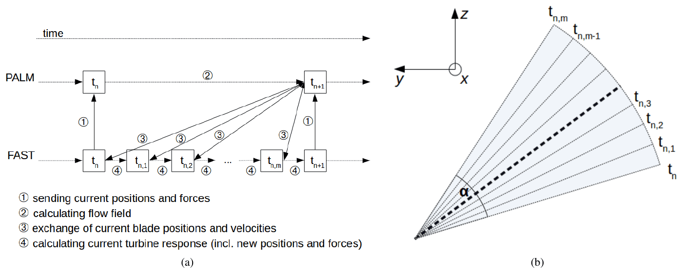
Figure 1 Schematic of the operation mode of the PALM–FAST ASM coupling. (a) Schematic of the PALM and FAST time stepping. (b) Schematic of one circle segment of the ASM. The values of the bold central line are used for the projection of the forces into the flow. Here, y and z denote the rotor plane and x the streamwise direction.

FAST therefore receives wind speeds of this frozen wind field and calculates the responding forces for the blades. During the larger PALM time step, the rotor blades cover a segment of the rotor area, a sector. The width of the sector α is calculated by the PALM time step Δt_P and the rotor speed Ω, which the FAST model communicates to PALM at the beginning of the PALM time step, using $\mathit{\alpha }=\mathrm{\Omega }\cdot \mathrm{\Delta }{t}_{\mathrm{P}}$. During the time step of PALM, several calculations of FAST are performed, similar to the schematic in Fig. 1b. Except the values of the bold central line, the information of the forces at the positions of the neighbouring lines is not used in PALM but is output in FAST. The values of the bold central line are used for all of the m lines in the sector, as in Fig. 1b. For each line a Gaussian-shaped smearing is calculated and projected into the model domain.

This smearing of the forces is realised by a polynomial resulting in a Gaussian shape that distributes the forces over the area surrounding the rotor blade in all three direction of space (Sørensen et al., 1998):

$$\begin{array}{}\text{(1)}& \mathit{\eta }={\displaystyle \frac{\mathrm{1}}{{\mathit{\epsilon }}^{\mathrm{3}}{\mathit{\pi }}^{\mathrm{3}/\mathrm{2}}}}\cdot \exp \left[-{\left({\displaystyle \frac{r}{\mathit{\epsilon }}}\right)}^{\mathrm{2}}\right],\end{array}$$

where η is the so-called regularisation function which is applied at the nodes of the grid within a certain vicinity of the turbine, r is the distance between the respective node and the blade element from which the respective force stems, and ε is a factor of the grid size that is typically set to $\mathit{\epsilon }=\mathrm{2}\cdot \mathrm{\Delta }$ (Troldborg, 2008), with Δ being the grid size.

In general, the forces acting on the blades are calculated based on the wind speed that is present at the blade position, i.e. the positions in the rotor plane. However, this wind speed does not represent the actual wind speed entirely as it depends on the grid resolution and has to be interpolated to the desired positions. Close to the last known blade positions this interpolation leads to higher wind speeds than in reality, which leads to an overestimation of the power output. Additionally, the projection width of the forces, i.e. the width defined by the regularisation function, influences the wind speed close to the blade immensely. To circumvent these issues, we take the wind speeds for the ASM in positions upstream of the turbine.

Far enough upstream of the rotor, the flow can be assumed to be almost undisturbed by the rotor. The wind speeds at the rotor area are then estimated using the induction model SWIRL of FAST. SWIRL uses the so-called Taylor frozen turbulence hypothesis (Taylor, 1938) and calculates the induced velocity in axial and tangential direction. In Moriarty and Hansen (2005) the AeroDyn model of FAST is described, including the blade-element momentum theory to compute the induction. The calculation of the induction factors when using SWIRL is based on Harman (1994). With enabling SWIRL we assume that the turbulent structures in the wind field do not change while moving to the turbine. In the current coupling a temporal change of the wind field as it approaches the rotor is not included. A comparison of different approaches, including the enhanced coupling described here, was done in Doubrawa et al. (2020) to simulate site-specific behaviour of a turbine. Besides LES, the discussed models also included Reynolds-averaged Navier–Stokes (RANS) simulations and were compared with respect to turbine output and wake data in different atmospheric stabilities. The models performed differently depending on the simulation of the inflow conditions and the resolution used. Especially for the neutral case our coupling showed very good results.

3 Validation

The validation of the coupling is divided into two parts. The first part is the evaluation of results using the generic NREL 5 MW turbine. The second part is the comparison to measurement data for a more extended analysis, for which a non-generic turbine is simulated.

3.1 Evaluation of the coupling on the basis of the generic NREL 5 MW turbine

The NREL 5 MW turbine (Jonkman et al., 2009b) is a generic turbine which has been used extensively in simulations (Churchfield et al., 2012; Storey et al., 2013, 2015; Vollmer et al., 2016; Sathe et al., 2013; Lee et al., 2012). The NREL 5 MW turbine was developed by the National Renewable Energy Laboratory (NREL), and a FAST model of the turbine is included in the FAST repository.

As this is a generic turbine, no comparison with measured data is possible. But the availability of the turbine data allows an evaluation of our enhanced coupling method, also in terms of turbulent flows. Additionally, the availability of the turbine data offers the opportunity to compare different methods and their computational resources. Therefore, two cases were considered, firstly a laminar and secondly a turbulent flow.

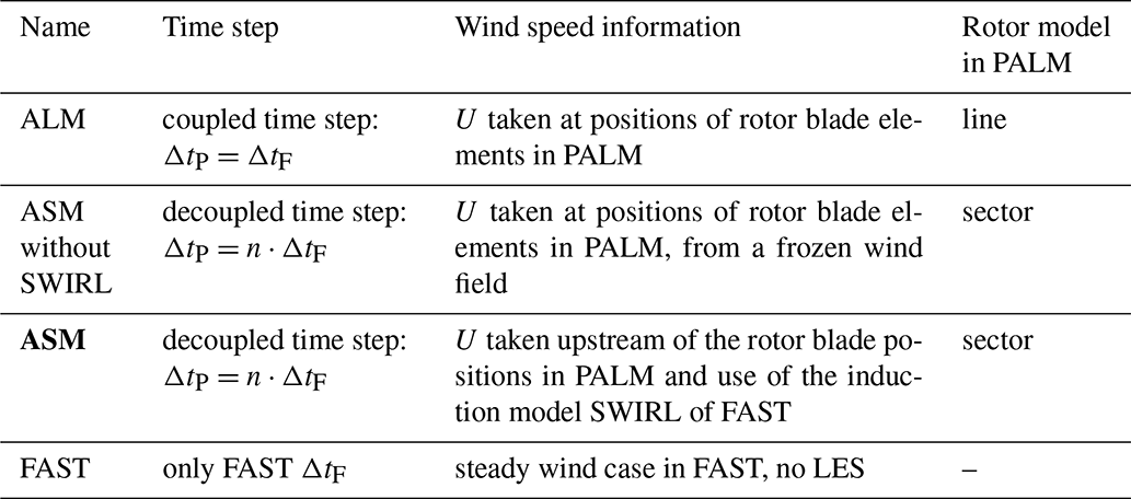
A comparison of four different methods is made, as summarised in Table 1. This includes a transient coupling between FAST and an ALM in PALM, meaning the same time step size in FAST and PALM (abbreviated as ALM). Furthermore, the ASM with two different modes of retrieving the wind speed is used, namely the ASM with the described method of reading out wind speeds in front of the turbine in combination with the induction model SWIRL (denoted as ASM), as well as taking the wind speeds at the rotor area without any induction model (denoted as ASM without SWIRL). As the fourth method, just in the laminar case, FAST on its own is used (denoted as FAST). For FAST on its own, the inflow wind option is set to match the PALM simulations; i.e. the power law variables are set to a wind speed of 8 m s⁻¹ constant with time and with height.

Table 1 Overview of the turbine models that were used in the comparisons. The new enhanced coupling method is ASM, the respective time steps in PALM and FAST are denoted as Δt_P and Δt_F respectively, and the inflow wind speed is denoted as U. The coupled model that is the focus of this paper is highlighted in bold.

To evaluate the different methods, at first, a laminar case with a constant wind speed with height, i.e. zero vertical gradient of the streamwise velocity, is considered. The LES simulations use a resolution of 5 m and 384 × 192 grid points in the flow direction and perpendicular to the flow direction. In the vertical direction, 192 grid points and a stretching are used, resulting in a total domain height of 3359 m. A larger model domain of 384 grid points perpendicular to the flow direction was tested as well to determine whether the size of the model domain influences the results. However, no significant differences in the conditions of the flow in the turbulent case (i.e. a deviation of 2 % in the wind speed at 92 m) or the turbine output were detected, and therefore the smaller model domain was used for the simulations. The boundary conditions at the inflow and outflow are set to cyclic; however, only the time at which the wake does not affect the inflow yet was evaluated. Additionally, the surface condition is set to a free-slip condition. PALM offers different possibilities for the subgrid-scale turbulence closure. For the simulations mentioned in this work the default model was used, which is a modified version of Deardorff's subgrid-scale model (Deardorff, 1980), as mentioned in Moeng and Wyngaard (1988) and Saiki et al. (2000). The time stepping and advection schemes were used in the default settings as well, which is a third-order Runge–Kutta scheme (Williamson, 1980; Baldauf, 2008) for time stepping and a fifth-order upwind scheme, based on Wicker and Skamarock (2002), for the advection. The pressure solver was set to the multigrid option (Uhlenbrock, 2001). The wind speed in the flow is set to 8 m s⁻¹. The inflow conditions for FAST are set accordingly. The standard controller of the NREL turbine is employed as described in Jonkman et al. (2009b), which means that at the prevailing wind speeds no pitching of the blades is enabled.

In Fig. 2, a comparison of the generator power for the generic 5 MW NREL turbine is shown. The ALM and ASM without SWIRL result in too high a power output, which is assumed to be, most importantly, due to the wind speeds used to calculate the blade response which is taken in the rotor plane. A further difference can be seen in the projection of the forces, which leads to different shapes of the simulated rotor. As described above, in the rotor area there is the danger of reading out velocity values that are too large. The ASM bypasses this issue by using the SWIRL induction method and results in a generator power which corresponds well with the expected one. The ASM without SWIRL shows an even higher power output than the ALM. The reason for that may be that in the ASM without SWIRL the area that is blocked in the rotor area is larger than for ALM, which might result in higher wind speeds in between the sectors, like a nozzle. As the wind speeds next to the projected forces are used to calculate the turbine response, these higher wind speeds would lead to a higher power output.

A comparison of quantities along the 62 blade nodes shows a difference between the methods using wind speeds at the rotor blade positions (ALM and ASM without SWIRL) and the two methods using a different inflow, namely ASM and FAST (figures can be seen in Appendix A). The distribution of the angle of attack shows a smoothed curve for the ALM and ASM without SWIRL, which is due to the smearing of the forces around the rotor blades. On the other hand ASM and FAST show a choppy curve due to the different airfoil profiles along the blade; here, it can be seen at which position a change of an airfoil profile and twist angle along the blade is predefined in the NREL model. These differences are transferred to the lift and drag coefficients. Additionally, for dynamic pressure, it can be observed that ALM and ASM without SWIRL overestimate the dynamic pressure at the blade tips and slightly underestimate it at the hub compared to FAST and ASM. These observations suggest that the smearing of the forces has a great influence on the lift and drag properties and thus the turbine response.

As a second case a turbulent flow is calculated. However, no comparison to FAST alone is done here since there is no literature value available to compare the results with. For the turbulent case, a neutral flow is simulated with neither heating nor cooling of the surface. A resolution of 4 m is used with 1200 × 480 grid points in the flow direction and perpendicular to the flow direction. In the vertical direction 192 grid points and a vertical stretching are used again, resulting in a vertical height of 1728 m. The roughness length is set to 0.05 m; the wind speed at hub height is about 7.4 m s⁻¹. In this simulation non-cyclic boundary conditions are used. If cyclic boundary conditions were used, the wake of the turbine would be fed into the inflow again and would, therefore, distort the flow in front of the turbine. In order to avoid this, PALM offers the opportunity of non-cyclic boundary conditions and a turbulence recycling method; for more information, see Maronga et al. (2015).

Figure 3 shows the time series of the generator power. The wind speeds in the ASM are taken 2D in front of the turbine, which in this example is a distance of 252 m, resulting in a time shift of the flow reaching the turbine of about 34 s. Therefore, when comparing the turbine output the result of the ASM simulation is shifted by 34 s for a better comparison to the other results. This does not affect the statistics but is a simple method to make the time series obtained from the different models comparable to each other. A model or tool that automatically fixes this time shift is not included in the current version of the coupling.

As for the laminar case, the ASM leads to a lower power output than the other models, whereas the differences are comparable to the laminar case in Fig. 2. Also, roughly the same peaks and therefore structures of the flow are present in the ASM results. This indicates that the coupling also works in a turbulent environment insofar as the turbulent structures are reflected in the power output.

Furthermore, these simulations are used to compare the computational times of the ALM and ASM. In the laminar case the ASM is 9 times faster than the ALM while using the same amount of cores; i.e. the computational time is reduced by up to 89 %. The turbulent case is calculated with a difference in the allocated cores: the ALM uses 4 times more cores than the ASM; however, the ASM is still about 3.5 times faster than the ALM. Consequently, the ASM provides the same set of output parameters as the ALM but is significantly faster.

Through these simple simulations it can be seen that the sector methods offer savings in the computing time in comparison to the ALM. However, the ASM without SWIRL does not provide the expected results. Therefore, it is considered useful to compare the ASM with measurement data in the following.

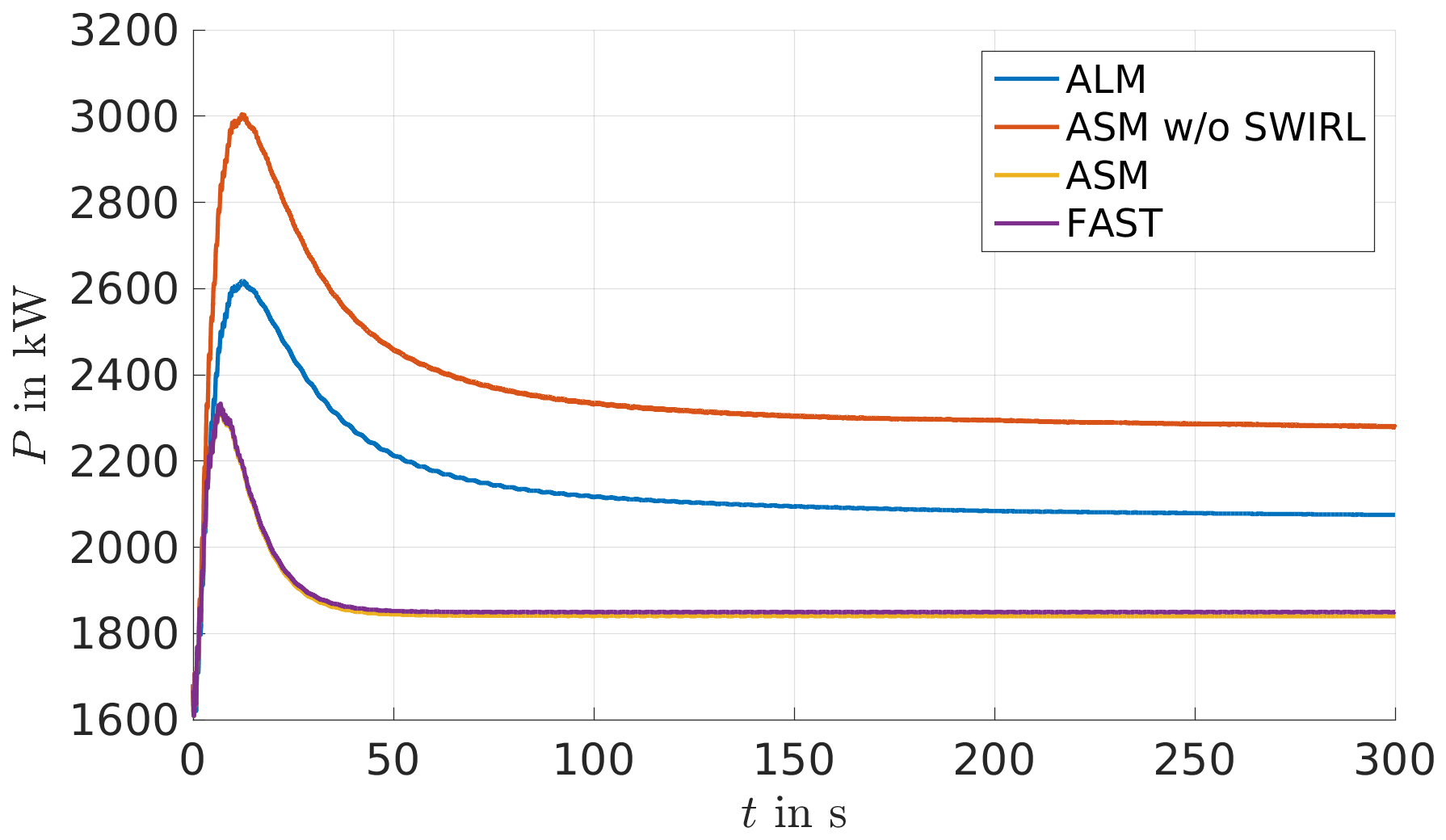
Figure 2 Comparison of different simulation methods for the generator power of the 5 MW NREL turbine in a laminar flow with 8 m s⁻¹ wind speed.

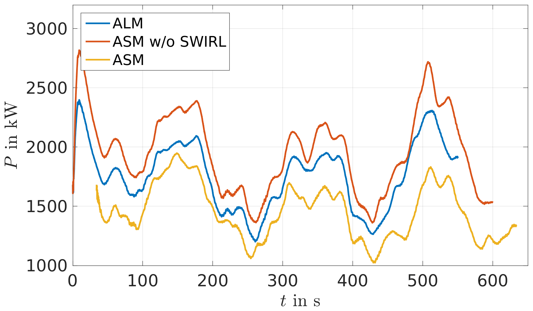
Figure 3 Comparison of different simulation methods for the generator power of the 5 MW NREL turbine in a turbulent flow at about 7.4 m s⁻¹ wind speed at hub height.

3.2 Validation of the coupling with the eno114 3.5 MW turbine

As the generic NREL 5 MW does not allow for a comparison to measurement data, a free-field turbine is used for further analyses. Measurement data of an eno114 3.5 MW turbine, manufactured by eno energy (eno energy, 2019), with a hub height of 92 m and the corresponding FAST turbine model are used for further investigations.

First, we consider laminar cases with uniform wind speed over height for the eno114 3.5 MW in order to establish a power curve. The reference power curve is obtained from stand-alone FAST runs, with a laminar inflow. The FAST turbine model is provided by eno energy, but the source code of the turbine controller was not available to us; only an executable file was provided. The calculated reference power curve coincides well with the published power curve of eno energy (eno energy, 2019), without figure. Of the published power curve no further information on the computation or data is available, and therefore no comparative plot is possible. For a wind speed of 8 m s⁻¹ the different models are compared again (see Fig. 4). The ALM again shows a higher power output than the reference power curve; the ASM coincides with the reference value and therefore with the value published by eno energy. The ASM without SWIRL shows again a higher power output than the ALM, although the difference is not as significant as in the laminar case of the NREL 5 MW turbine (see Fig. 2).

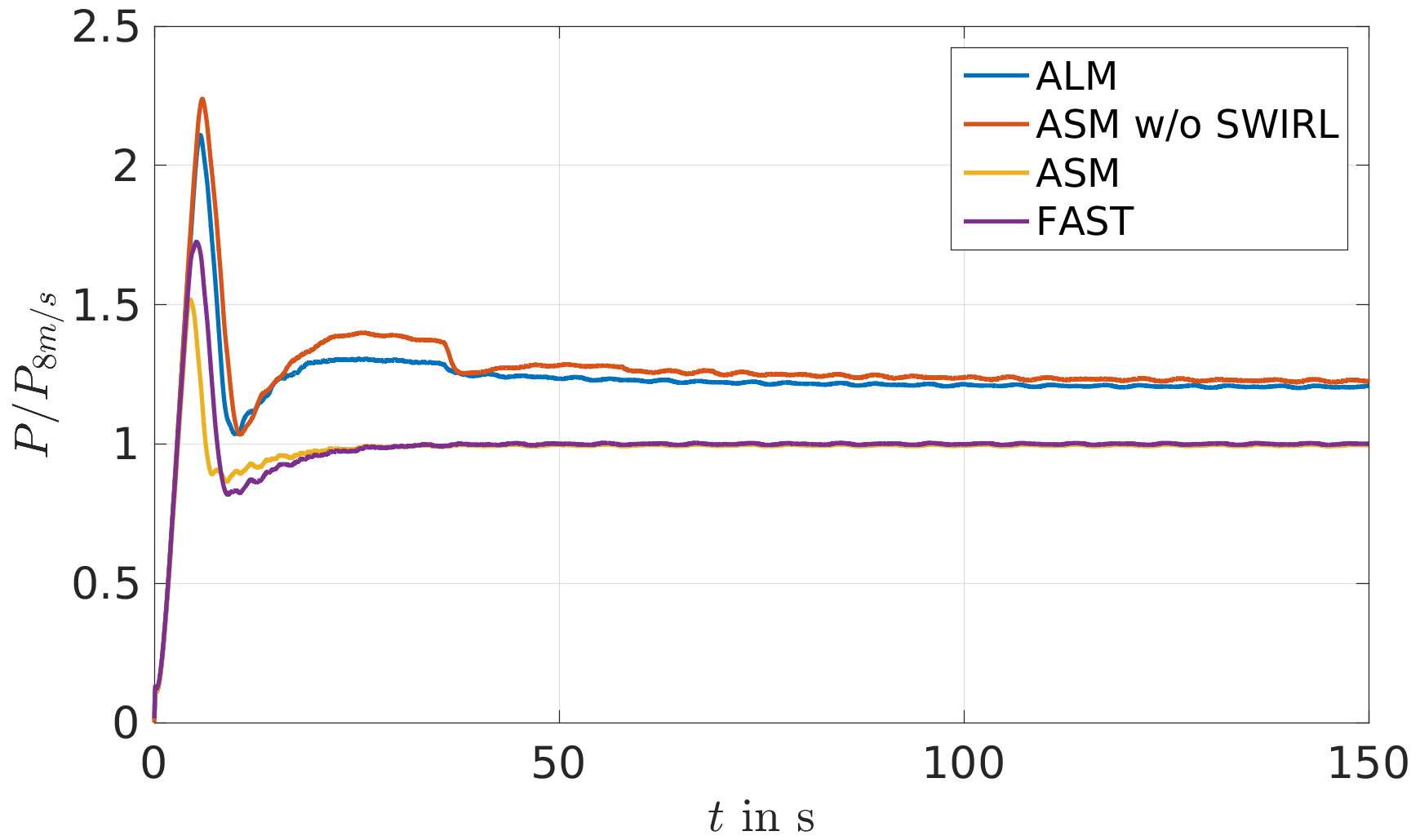
Figure 4 Comparison of different simulation methods for the generator power of the eno114 3.5 MW turbine in a laminar case with a wind speed of 8 m s⁻¹, normalised by the respective value of the eno114 3.5 MW energy power curve at 8 m s⁻¹.

3.2.1 Conditions at the onshore measurement site near Brusow

The onshore measurement site, from which data were available, is situated in northern Germany close to the village of Brusow. At the measurement site two eno114 3.5 MW turbines are present. For one turbine (turbine 1 in Fig. 5) measurement data were available, consisting among others of the power output, rotor speed, generator speed and tower, main shaft, and blade root bending moments.

Apart from the two eno energy turbines the measurement site was also equipped with a met mast. Figure 5 shows the general set-up of the site. The met mast contained three cup anemometers, one wind vane and one eddy-covariance station of the IRGASON type from Campbell Scientific. The cup anemometers were situated at the heights 34.6, 89.3 and 91.5 m; the wind vane was situated at 89.3 m; and one of the eddy-covariance stations was situated at 34.6 m. Another eddy-covariance station was located at a height of 2.3 m on the boom of a separate tripod that was situated next to the met mast.

From the 20 Hz data provided by the eddy-covariance stations, turbulence statistics with a resolution of 30 min are obtained by applying the eddy-covariance software TK3 (Mauder and Foken, 2015). The planar fit method (Wilczak et al., 2001) is used for correcting impacts of a tilted device on the turbulence statistics. For calculating the planar coefficients, the whole available data set is taken into account. As the IRGASON is not an omnidirectional device, planar fit coefficients are calculated for four different wind direction sectors as suggested by the manufacturer of the IRGASON. The distance of the met mast to the turbine, for which measurement data are available, was 280 m (≈ 2.5D) in the 190^∘ direction, referring to the wind turbine.

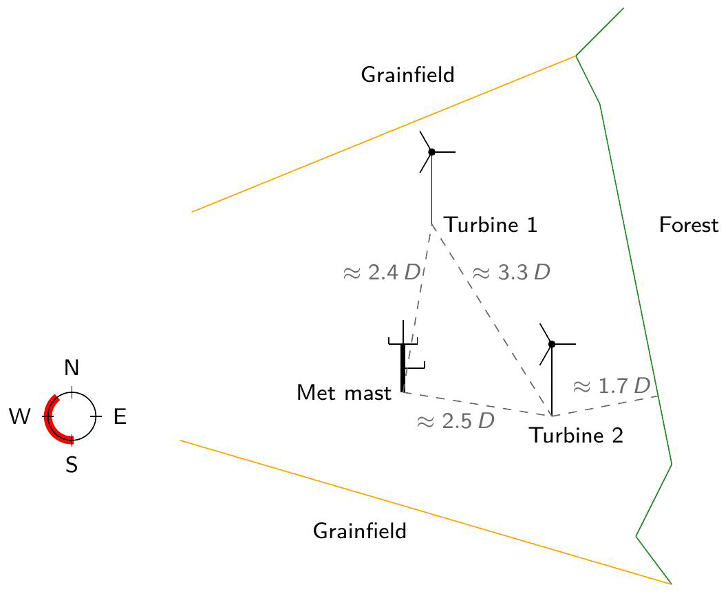
Figure 5 Schematic of the measurement site in Brusow. The remaining wind directions in the measurement data, after filtering, are indicated in red; D is the turbine diameter, here D=114.9 m.

Data of all sensors is available from 10 May until 30 June in 2017. To the east of the site of the turbines and met mast a forest is located, which influences the measurements greatly. Therefore, the measurement data are filtered for the westerly wind directions, where mostly grainfields are situated.

We estimate the roughness length of the surrounding area using the wind speed u_ec and the friction velocity u_*, both provided by the lower eddy-covariance station, with Eq. (2) for data of neutral stratification, where k is the von Kármán constant, z_ec the height of the respective eddy-covariance station and z₀ the desired roughness length:

$$\begin{array}{}\text{(2)}& u_{\mathrm{ec}}={\displaystyle \frac{u_{*}}{\mathrm{k}}}\ln \left({\displaystyle \frac{z_{\mathrm{ec}}}{z_{\mathrm{0}}}}\right).\end{array}$$

The plot of the roughness length distribution (Fig. 6) shows an approximate roughness length of z₀=0.1 m for the westerly region. This value corresponds to farmland and hedges in the summer time according to Stull (2003), which is in agreement with the plants on-site, and therefore z₀=0.1 m is a reasonable value for the roughness length.

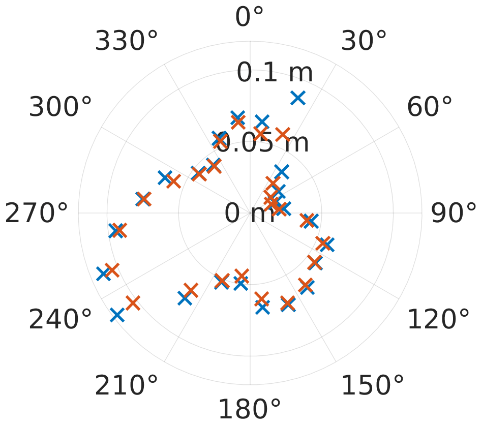
Figure 6 Roughness length distribution for varying wind directions for the measurement period. Two methods of averaging the roughness length values gained by Eq. (2) were used; here z₀ denotes the roughness length determined from 30 min eddy-covariance data, and j denotes the 15^∘ wind direction bins: (1) averaging z_0,j per 15^∘ bins (blue) and (2) averaging using $\ln z_{\mathrm{0},j}=\frac{\langle u_{*}\ln \left(z_{\mathrm{0},j}\right)\rangle }{\langle u_{*}\rangle }$ per 15^∘ bins (red), where the angle brackets 〈…〉 denote the average over values within the 15^∘ bins.

From the data of the eddy-covariance stations the stability parameter $\frac{z}{L}$, with z as the measurement height, here z_ec, and L the Obukhov length are obtained from the application of the software TK3 to them. In the following, the power that was produced during the respective times is plotted with respect to the wind speeds filtered by the stability, calculated from the data collected by the eddy-covariance stations. For that, the 50 Hz measurement data of the power are averaged over 10 min intervals, denoted as P₁₀. These 10 min power values are sorted according to stability and wind speed and averaged according to the wind speed within the respective stability, resulting in ${\stackrel{\mathrm{‾}}{P}}_{\mathrm{10}}$. For normalisation the maximum 10 min power value P_10 max is used. Accordingly, the standard deviation is calculated; i.e. the standard deviation is calculated for 10 min intervals ${\mathit{\sigma }}_{P_{\mathrm{10}}}$, and then these 10 min values are averaged according to their stability and wind speed ${\stackrel{\mathrm{‾}}{\mathit{\sigma }}}_{P_{\mathrm{10}}}$ and normalised with the maximum 10 min standard deviation value ${\mathit{\sigma }}_{P_{\mathrm{10}\max }}$.

Figure 7 shows the resulting power data analysed with respect to the stability and normalised by simulation data of FAST, which coincides with the values provided by eno energy for the 3.5 MW turbine (cf. eno energy, 2019). Due to the relatively low number of measurements, the stabilities, based on the data of the lower eddy-covariance station of z_ec=2.3 m, are sorted to stable ($\frac{z}{L}>\mathrm{0.0115}$), neutral ($-\mathrm{0.0115}<\frac{z}{L}<\mathrm{0.0115}$) and unstable ($\frac{z}{L}<-\mathrm{0.0115}$) but not for further classification in very stable and very unstable (Table 2).

It can be seen that the measurement data deviate only slightly from the simulation data. Also, no clear trend between the different stratifications can be observed. Differences for the stratifications can be seen in the turbulence intensity and the shear (see Figs. 9 and 10). As expected the unstable cases have a higher turbulence intensity (TI) than the stable cases. This is also visible in the standard deviation of the power (see Fig. 8), as the higher TI in the neutral and unstable case leads to a higher standard deviation of the power than in the stable situations with lower TI.

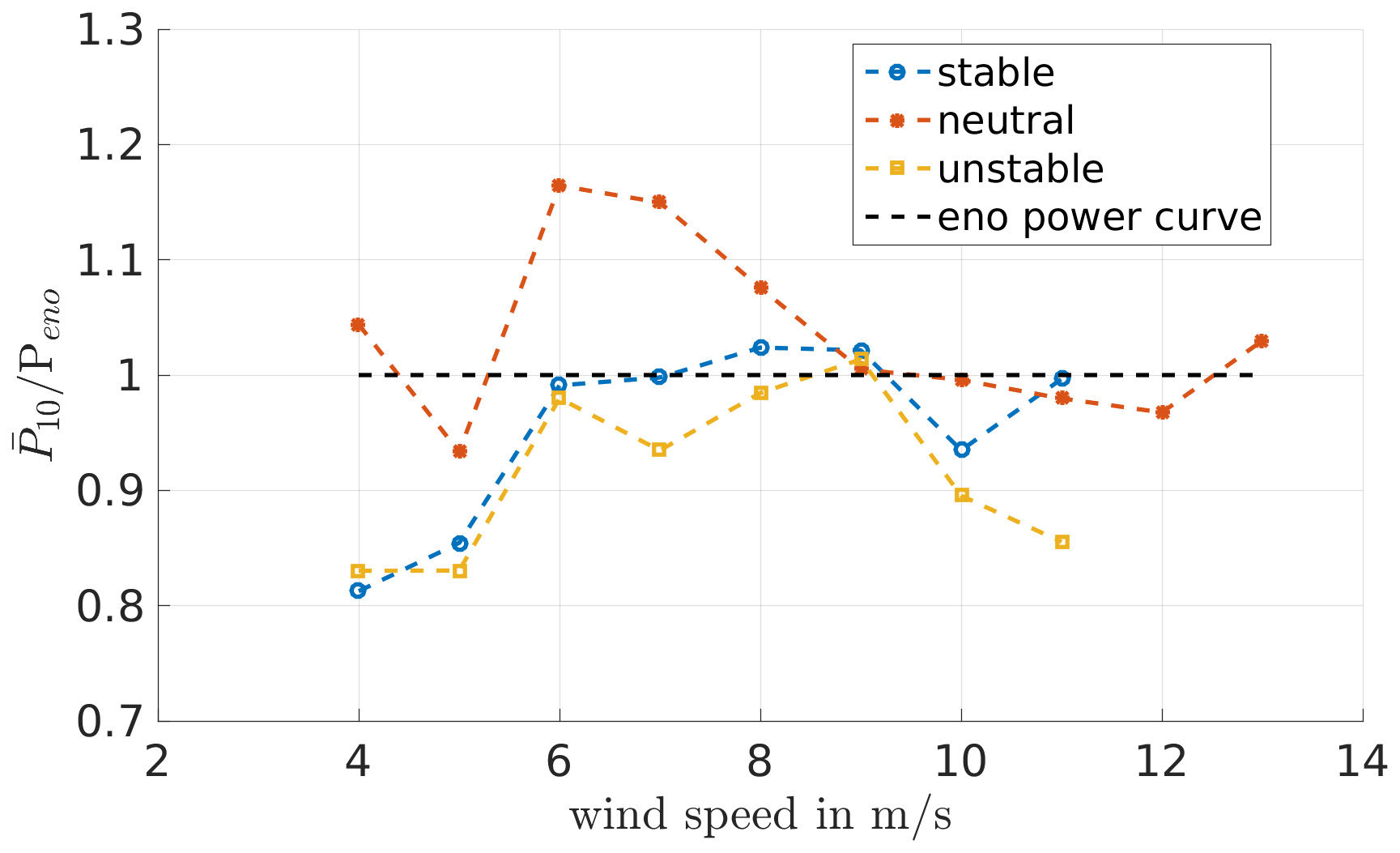
Figure 7 Power data determined from the measurement data for May/June 2017, normalised by the corresponding power of the eno114 3.5 MW power curve determined by FAST in laminar conditions, for different stabilities (determined from eddy-covariance data).

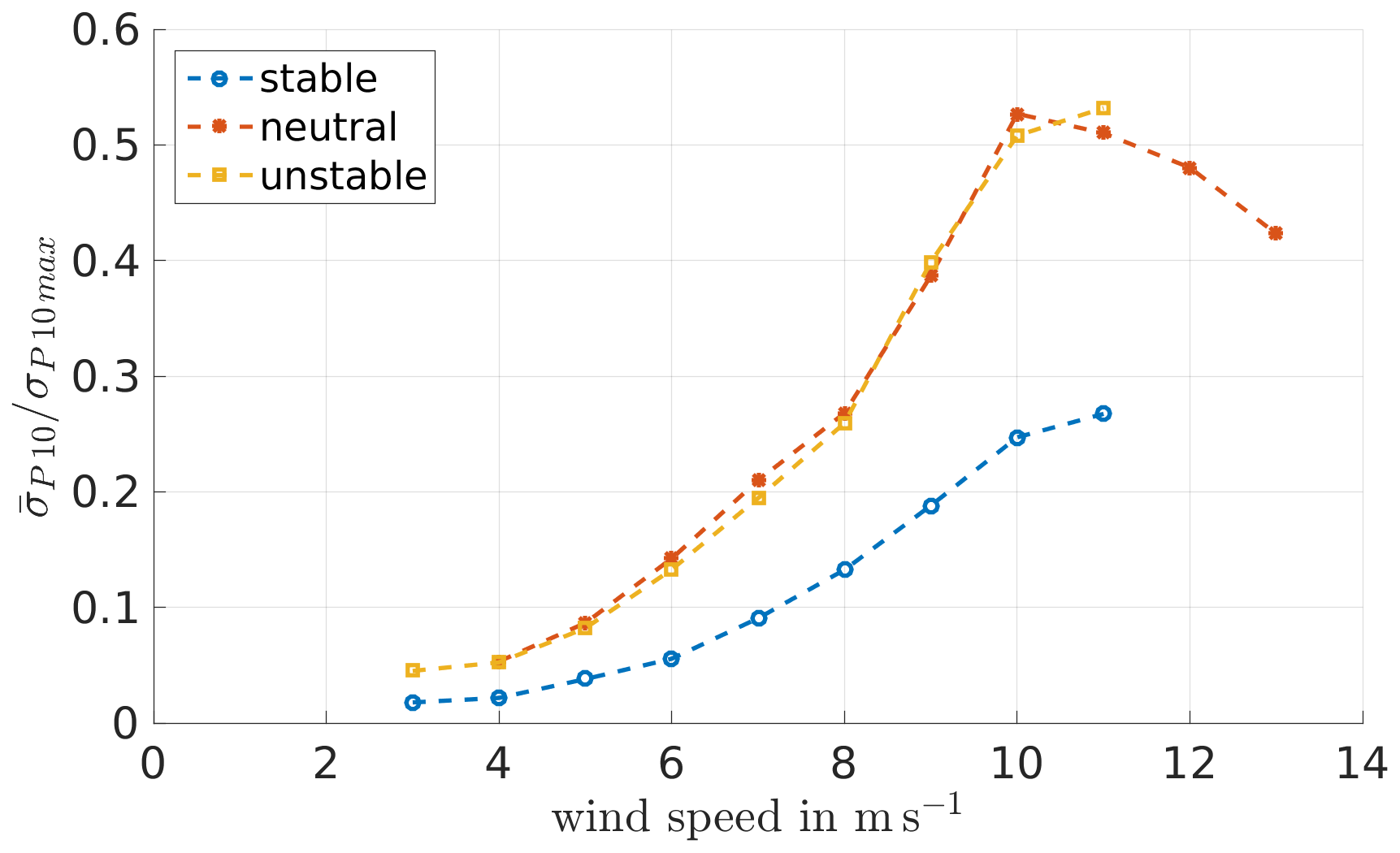
Figure 8 Standard deviation for 10 min intervals of the measured turbine power output, calculated according to ${\mathit{\sigma }}_{P_{\mathrm{10}}}=\sqrt{\frac{\mathrm{1}}{N_{\mathrm{meas}}-\mathrm{1}}\sum _{k=\mathrm{1}}^{N_{\mathrm{meas}}}{\left|P\left(t_k\right)-P_{\mathrm{10}}\right|}^{\mathrm{2}}}$, where P(t_k) denotes the power data measured in 50 Hz, P₁₀ the 10 min average and N_meas the number of measurements within the 10 min interval, normalised by the maximum 10 min standard deviation of the power, for May/June 2017, and sorted and averaged according to stability (determined from eddy-covariance data) and wind speed.

Table 2 Classification of atmospheric stability according to Obukhov length L, based on Peña et al. (2008). The distribution of the atmospheric stability in the measured data can be seen in Figs. 9 and 10.

3.2.2 Simulation set-up for Brusow

In the following, the simulation set-ups for PALM and FAST that are used for the comparison to the measurement data are described.

PALM

In order to compare simulation results to the measurement data, simulations are computed that result in flow conditions similar to those observed under neutral boundary layer (NBL) and stable boundary layer (SBL) flow at Brusow. As can be seen in Figs. 9 and 10 most data are available for the NBL and slightly SBL.

Precursor simulations without a turbine are performed in order to reach a stationary state and evaluate the produced inflow conditions prior to the main simulations containing a wind turbine. The resolution for both neutral and stable conditions is set to 4 m in the x and y direction and in the vertical direction up to a height of 600 m. Above z=600 m a vertical stretching of the grid with a factor of 1.08 is used. In accordance with the results of our evaluation of the roughness length from eddy-covariance data at the site, the roughness length z₀ is set to 0.1 m (see Fig. 6). A homogeneous roughness length is set in the model domain, and no topography is taken into account, which means that idealised simulation conditions are used. In Table 3 the different set-ups and in Table 4 the resulting flow conditions are shown.

Table 3 Set-up of the precursor simulations: size of the model domain in the streamwise x, spanwise y and vertical z direction; grid size Δ; cooling rate $\mathrm{\Delta }\mathrm{\Theta }/\mathrm{\Delta }t$; geostrophic wind speed components at the surface in the x and y direction u_g and v_g; and total simulated time t_end.

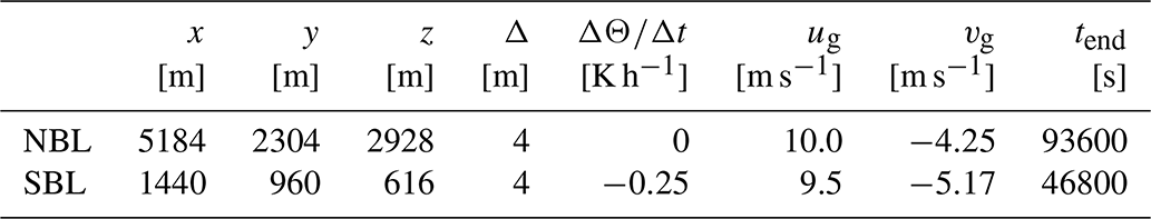
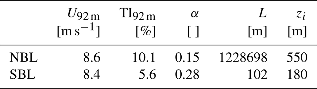
Table 4 Resulting flow parameters after reaching a stationary state in the precursor simulations, averaged over 3600 s: the magnitude of the wind speed at hub height averaged over the model domain U_92 m, turbulence intensity calculated at one position in 92 m height TI_92 m, shear parameter α (based on the power law $u_{\mathrm{2}}=u_{\mathrm{1}}{\left(\frac{z_{\mathrm{2}}}{z_{\mathrm{1}}}\right)}^{\mathit{\alpha }}$ for the relation of wind speeds at different heights), Obukhov length L in a height of 2.3 m and boundary layer height z_i.

For the respective main runs including the turbine a larger model domain and non-cyclic boundary conditions were used to avoid influences of the wake onto the turbine. The model domain of the neutral case is larger than the one of the stable case, as in neutral conditions the turbulent structures tend to be larger than in stable conditions: the neutral model domain is set to 7680 m × 2595 m × 2928 m, and the stable is set to 5760 m × 2304 m × 616 m. The simulations are set up according to the simulations in Vollmer et al. (2016).

To reduce local effects caused by possible persistent structures in the flow, the main run is simulated three times with three different turbine positions in the y direction. Table 5 shows the differences of the flow between the turbine positions. The power output resulting from the simulations at the different positions is used to compare to the measured data, yielding three results for both stabilities as can be seen in Figs. 11 to 14.

Table 5 Turbine positions along the y axis (keeping the same x position), with the y direction spanning from 0 to 2595 m for the NBL and from 0 to 2304 m for the SBL, in the model domain of the main run; additionally, the local wind speed U_92 m and turbulence intensity TI_92 m at hub height at these y coordinates, taken 2.5D in front of the turbine averaged over the last 10 min of a 650 s simulation.

Figures 9 and 10 show how the precursor simulations, i.e. the inflow conditions for the turbine, compare to the measurement data. The crosses represent the data from the precursor runs, so the undisturbed inflow averaged over space, at height 92 m, and time. In comparison to the measurement data, both simulations, neutral and stable, are in the lower region of the measured turbulence and shear. However, the TI of the simulations is calculated using the resolved turbulence and disregarding the subgrid-scale one; hence, it is likely that the TI in the simulations is slightly higher than seen here. Therefore, the simulation set-up seems to resemble the inflow conditions at Brusow reasonably well. Since the flow conditions in the simulations match the measurements, the turbine output is compared in the following.

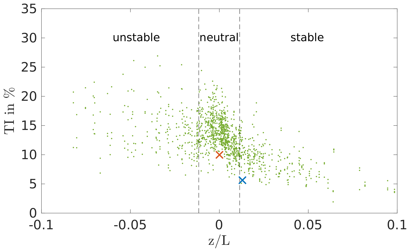
Figure 9 Turbulence intensity TI_92 m of the measurement data (green) in comparison to the resulting TI_92 m of the precursor runs sorted in neutral and stable (red – neutral; blue – stable).

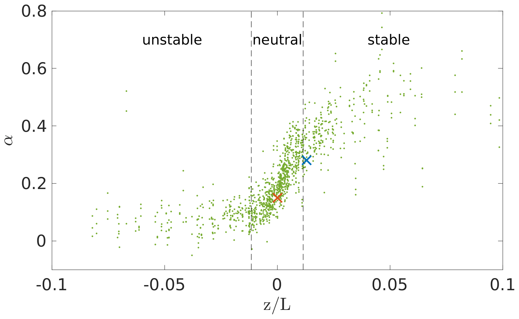
Figure 10 Shear of the measurement data (green) in comparison to the resulting shear of the precursor runs sorted in neutral and stable (red – neutral; blue – stable).

FAST

The turbine model of the eno114 3.5 MW turbine for FAST was provided by eno energy, including structural information and a pitch, a speed and a yaw control in the format of a Bladed .dll file, which was not accessible to us. However, the yaw of the turbine is neglected, as the flow in PALM was directed in such a way that the turbine is aligned with the wind. In FAST the modules ElastoDyn, AeroDyn and ServoDyn were used, and the degrees of freedom for the blade and tower were set to true except the rotor-teeter and yaw flag. All the platform degrees of freedom were neglected, i.e. set to false. The time step throughout all modules was set to Δt=0.01 s. In AeroDyn the Beddoes–Leishman dynamic stall model, based on Leishman and Beddoes (1989) and the “Equil” option, a blade element momentum (BEM) theory model, for the inflow was selected. Additionally, the tip-loss and hub-loss models were enabled and set to the Prandtl tip-loss model (Prandtl and Betz, 1927).

3.2.3 Comparison of the turbine data

In the following plots the output data of the turbine in the simulations are compared to the measurement data. The main runs of the simulations are run for a simulation time of 650 s, and the results are averaged over 600 s, discarding the first 50 s as a spin-up of the turbine simulation; this time frame is derived from the laminar case (see Fig. 4). To compare the power output of the simulations to the measurement data, the power needs to be set into relation with the correct corresponding inflow wind speed. As the wind speed in Brusow is determined from a cup anemometer on a met mast at a distance of 2.5D from the turbine at hub height, in the simulation the wind speed is taken as well in a single point at a distance of 2.5D in front of the turbine position at hub height and averaged over time.

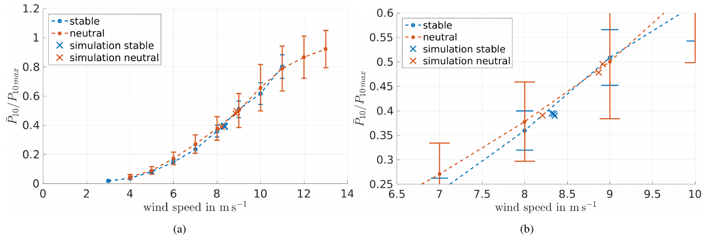
Figure 11 (a) Power curve, normalised by maximum 10 min power, determined from measurement data including standard deviation in comparison to the results of the simulation (marked by ×). (b) Enlargement of panel (a). The standard deviation is plotted again in Fig. 12.

In Fig. 11 the simulation results are shown in comparison to the power curve determined by the measurement data at hub height. The error bars show the standard deviation of 10 min means. Figure 11 shows the same plot enlarged at the wind speeds of the simulation. According to Dörenkämper et al. (2014), using offshore data, and Wharton and Lundquist (2012), using onshore data, slight differences of the power output depending on the atmospheric stabilities can be seen. However, both publications together do not show a clear trend of which stability generally leads to the higher power output. In an offshore environment, as in Dörenkämper et al. (2014), unstable conditions lead to a higher power output below rated wind speed, and at an onshore site (see Wharton and Lundquist, 2012) the stably stratified atmospheric boundary layer (ABL) yields the higher power output. However, different wind speeds were used as a reference, which makes a comparison of the results difficult. In Wharton and Lundquist (2012) a rotor equivalent wind speed was used, while Dörenkämper et al. (2014) used the measurement data of a met mast at 90 m height.

The measurement data of Brusow, with the wind speed at hub height as reference, does not show any clear tendency for the dependency of the wind turbine power on atmospheric stability (see Figs. 7 and 11). A power curve depending on the rotor equivalent wind speed was calculated from the measured data as well but does not conclude in a clear trend either. The rotor equivalent wind speed was computed according to Wagner et al. (2014), but due to the limited number of measurement heights and their irregular distribution over the height, the results could be prone to errors. Therefore, for further analysis the hub height wind speed is used. The apparent independence of the wind turbine power on atmospheric stability might be due to the limited amount of only 2 months of data that were available or might be depending on the measuring and classification of the stability. As shown in Wharton and Lundquist (2012) the stability-filtered power curve greatly depends on the measurement heights used for determining the shear. However, this behaviour is also not present in the simulations. Therefore, in our case, the power output is not the proper parameter to show different turbine responses depending on the atmospheric stability.

Figure 12 shows the standard deviation of the power with respect to the wind speed. Higher fluctuations of the power in the neutral cases can be observed, corresponding to the higher TI that is present in the neutral stratification (cf. Mittelmeier et al., 2017). The simulation data show a comparable behaviour with lower fluctuating power in the stable cases than in the neutral ones. In the three neutral simulations the distribution of the standard deviation is spread relatively wide compared to the stable cases. The three different positions that were used for the neutral simulations differ slightly in wind speed and TI, which is not the case for the stable cases (see Table 5).

To check whether this distribution is comparable to the measurement data, a plot of the standard deviation of the power with respect to the TI is made (Fig. 13). It shows the relation between the power fluctuations to the TI for all measured values (green dots) and specifically the measured stable and neutral cases (blue and red asterisks) and in comparison the respective values of the simulations (blue and red crosses). As shown in Fig. 13, the results of the simulations show realistic data, even though they are not centrally located within the measurement points; therefore, other turbine parameters available are compared. Specifically, the blade and tower loads are investigated below.

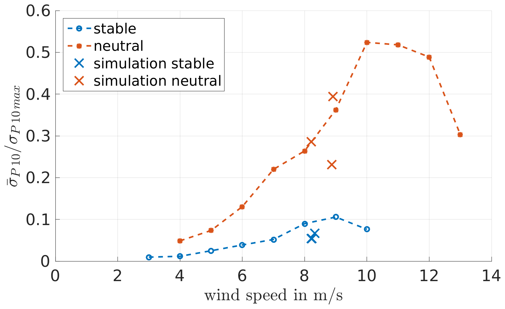
Figure 12 Normalised standard deviation of the power with respect to the wind speed determined from measurement data in comparison to the simulation results (×). Sorted into stability by eddy-covariance data, TI and shear determined from the met mast data.

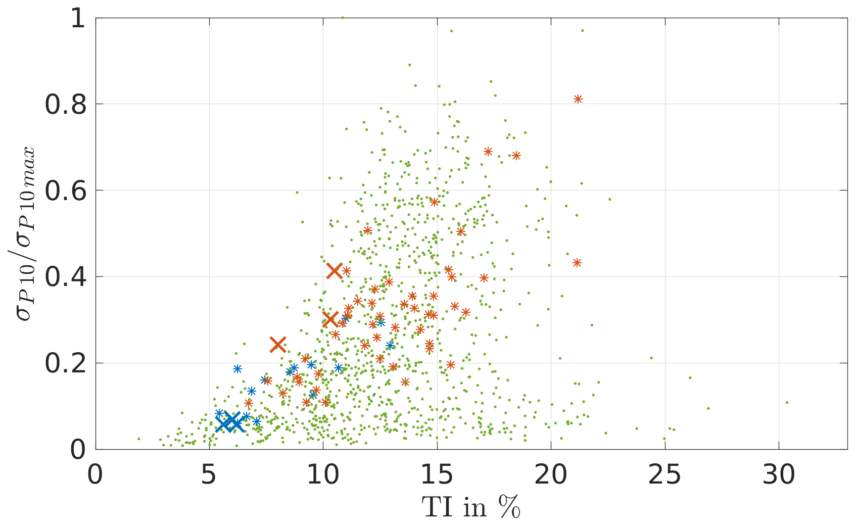
Figure 13 Standard deviation of the power with respect to the TI determined from measurement data (green – all wind speeds; blue and red asterisks – stable and neutral measurements at wind speeds of 8–9 m s⁻¹) in comparison to the simulation results (×).

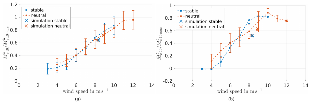
Figure 14 Blade root bending moment (a) out of plane $M_y^{\mathrm{b}}$ and (b) in plane $M_x^{\mathrm{b}}$ with respect to wind speed in comparison to the simulation results; averaged 10 min values were sorted by stability, averaged according to wind speed and normalised with the maximum measured moment.

The flap-wise and edgewise blade root bending moments are evaluated, but also data for the tower top and base loads are available and examined. Figure 14 shows the measured blade root bending moments with respect to the wind speed; the results of the simulations are indicated by crosses. The out-of-plane blade root bending shows a good agreement, and the in-plane blade root bending moment differs a bit more. However, a more suitable way to compare the loads is to look at the spectra.

We filtered the data with respect to westerly winds, stability and rotor speed. The analysis of the rotor speed showed a difference in the controller behaviour of the real system compared to the modelled one. This can be seen in Figs. 19 and 20, showing the measurements in Brusow. While Fig. 19 presents the relationship between the wind turbine power output and the rotor speed, Fig. 20 shows the relationship between rotor speed and wind speed. The combination of the respective values obtained from the simulations is provided by marks in these figures. Evidently, for the power output the values obtained for the simulation are within the standard deviation of the measurements that are indicated by bars. In that sense our set-up seems to be successful. We point out that we did not set up our simulations in such a way that they would lead to the reproduction of the mean behaviour of the wind turbine for the specific bins of measured data. We simulated just a few selected cases within the neutral and stable range of atmospheric stability. Thus, a deviation of the turbine response from the mean behaviour in the measurements can be expected. Note that the cases simulated by us are cases with a comparatively low turbulence intensity. We do not know the details of the controller of the wind turbine, so it is hard to verify any hypothesis for why our cases show a smaller rotor speed in comparison with the mean rotor speed for the next bin of measured data. Therefore, it is only possible to compare loads at either the same rotor speed or the same wind speed.

For the stable case some of the time intervals have to be discarded due to a varying quality of the load sensors, leaving one interval for the stable case where data are continuous for the blade and tower moments. For the neutral case the longest remaining interval covers a span 165 s long. The conditions of the chosen intervals are shown in Table 6. Ideally the chosen intervals should match the simulation parameters, but due to the described limitations in the measurement data, the remaining intervals can be seen as the best fit. These available cases suffice for the validation of our code. For an even more detailed load analysis, better fits might be necessary.

Table 6 Summary of the parameters of the measurement interval data used for the spectra of the blade and turbine loads: wind speed at hub height U_92 m, turbulence intensity at hub height TI_92 m, shear parameter α and the length of the available time interval t_interval.

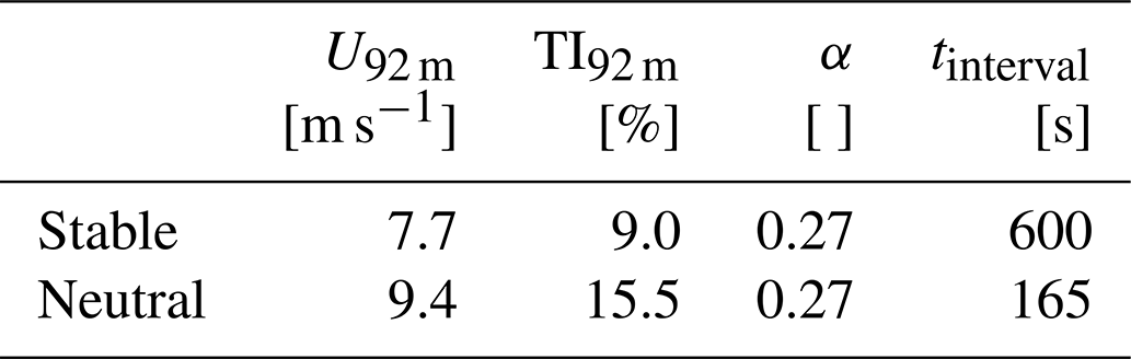
In the following the stable case will be discussed in detail. The neutral case also shows a good agreement between simulation and measurement data but covers only a short time interval of only 165 s; the corresponding spectra can be found in Appendix B.

Figure 15 shows spectra of the blade root bending moments for the stable case. Figures 16 and 17 show the resulting tower load spectra for the stable case.

The spectra of the blade root bending moments are normalised by the same maximum value from both moments. The spectra of the tower top and tower base bending moments are normalised with their respective maximum values as well. The frequency is normalised by the rotor speed Ω.

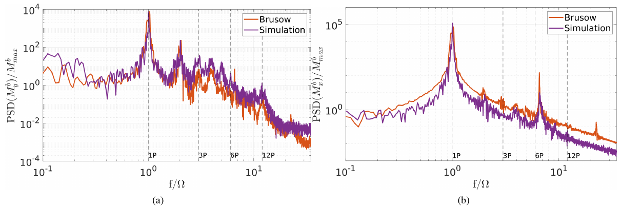
Figure 15 Spectrum of the blade root bending moment (a) out of plane $M_y^{\mathrm{b}}$ and (b) in plane $M_x^{\mathrm{b}}$ in comparison to the simulation results (stable). The data are normalised by the maximum value of the blade root bending moments.

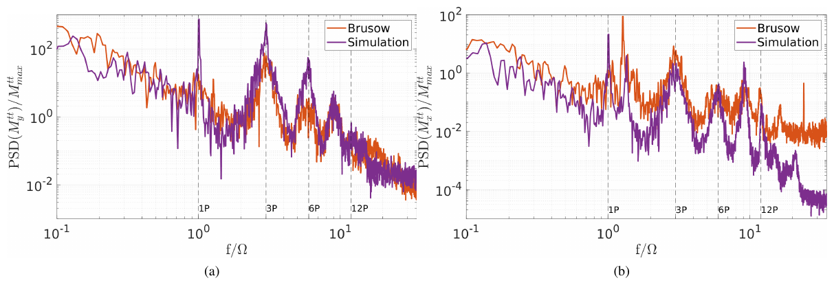
Figure 16 Spectrum of the tower top bending moment in (a) the fore-to-aft direction $M_y^{\mathrm{tt}}$ and (b) the side-to-side direction $M_x^{\mathrm{tt}}$; comparison of the measurement data to the simulation results (stable). The data are normalised by the maximum value of the tower top bending moments, and the frequency is normalised by the rotor speed.

In the spectra of the stable case it can be observed that the torsion loads show comparable results (see Fig. 17c). In addition, the fore–aft and side-to-side tower loads (see Fig. 16 and Fig. 17a, b) and the blade root bending moments (see Fig. 15) are represented well in the simulation. In general, most of the multiples of the rotor speed are represented in both the measurements and the simulations, and also their levels are comparable. The peaks show a difference in the width depending on the turbulence intensity; i.e. in the stable, less turbulent case the peaks are less wide than in the more turbulent, neutral case (figures in Appendix B). This can be observed both in the measurement data and the simulation results.

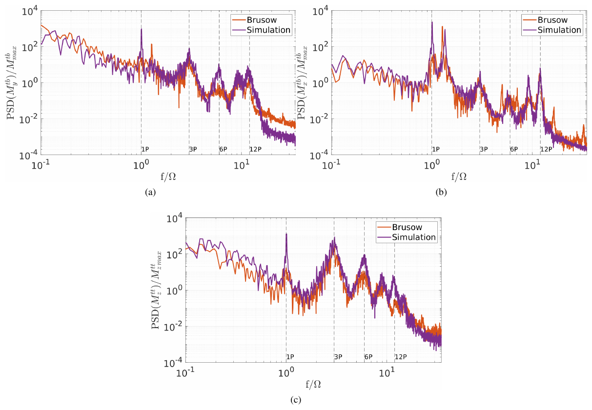
Figure 17 Spectrum of the tower moments: (a) the tower base bending in the fore-to-aft direction $M_y^{\mathrm{tb}}$, (b) the tower base bending in the side-to-side direction $M_x^{\mathrm{tb}}$ and (c) the tower top torsion $M_z^{\mathrm{tt}}$; comparison of the measurement data to the simulation results (stable). The data are normalised by the maximum value of the tower base and tower top torsion moment, and the frequency is normalised by the rotor speed.

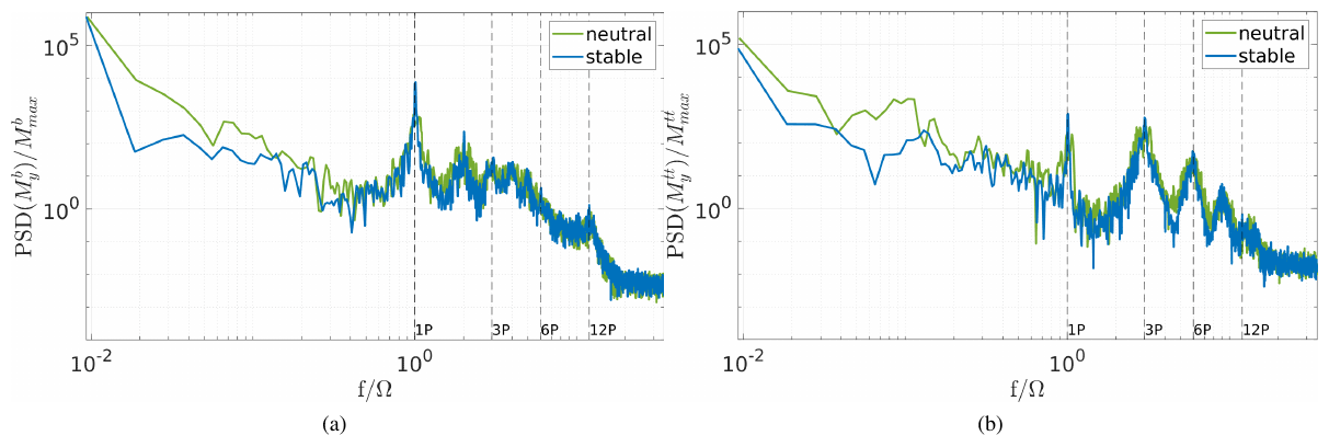
Figure 18 Comparison of the (a) blade root bending moments out of plane $M_y^{\mathrm{b}}$ and (b) tower top fore–aft bending moment $M_y^{\mathrm{tt}}$ for the stable and neutral simulation. The data are normalised by the maximum value of the blade root bending and tower top bending moments, and the frequency is normalised by the rotor speed.

It can also be seen that the 1P peak is of different height in the tower load spectra. The peak of the simulation data reaches higher than the one of the measurement data. This is probably due to an overestimated blade imbalance in the simulation which has been used to respect weight and pitch differences between the blades (cf. Zhang et al., 2015). In the FAST turbine model one of the blades has a 1 % higher mass density than the others, and also a pitch offset of 0.3^∘ is set between all three blades. This results in a very pronounced 1P peak that does not exist in the measurement data.

Notable is also that there seems to be a discrepancy between the simulation and measurement data in the tower top side-to-side bending moment in stable and neutral conditions. This might be caused by the difference in the tower model to the real behaviour of the turbine tower. It can be seen that the first tower eigenfrequency is slightly lower on the real turbine and therefore more prone to the rotational excitation. In the measurement data the first tower eigenfrequency is closer to the 1P peak, and therefore the vibrations are less damped. Differences can also be observed in the 6P peak, especially in Fig. 16. The 6P peak is greatly influenced by the shear and the wind speed differences across the rotor area. A plot of the wind speed profiles can be found in Appendix C; even though the shear is similar, the difference in the wind speeds, which are caused by the above-described limitations in the measurement data, led to diverging wind speed profiles. In Fig. 18 a comparison between the neutral and stable simulation results for a blade root bending and tower bending moment is shown. The bending moments that are mostly affected directly by the flow, i.e. by the thrust, are chosen. It can be observed that the neutral simulation leads to wider peaks due to the higher TI and the resulting varying rotor speed. Also, a difference in the height and depth of some peaks can be seen. Namely for the blade root bending out-of-plane moment the 2P and for the tower fore–aft bending moments the 3P and 6P peaks are higher and reach further down for the stable case than the neutral case. These multiples of the rotor speed are influenced by the shear of the flow which also indicates a difference in the inflow of the turbines.

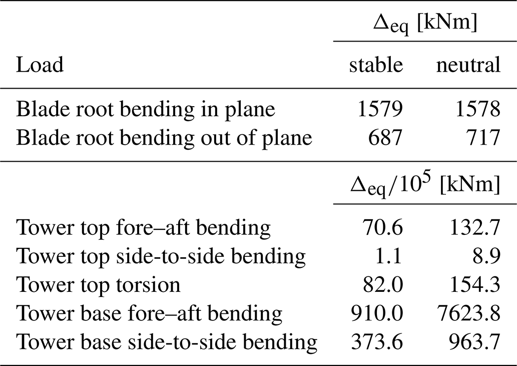
To investigate the loads further, rain flow counts and the value of the equivalent load range Δ_eq (non-normalised damaged equivalent loads (DEL)) were calculated. Equation (3) shows the used Palmgren–Miner rule, taken from Vera-Tudela and Kühn (2017):

$$\begin{array}{}\text{(3)}& {\mathrm{\Delta }}_{\mathrm{eq}}={\left(\sum _{k=\mathrm{1}}^{\mathrm{n}}{N}_k\mathrm{\Delta }{S}_k^m/N_{\mathrm{ref}}\right)}^{\mathrm{1}/m},\end{array}$$

where n is the number of different loading amplitudes, N the number of cycles and ΔS the loading amplitude. Further, a Wöhler exponent of m=10 for the blades, m=4 for the tower and a reference number of cycles N_ref=10⁷ is assumed.

A comparison between the measurement data and the simulation results is not useful in this case as the available intervals vary in their inflow parameters and therefore the rotor speed. However, a comparison between the results of the simulation of the neutral and stable boundary layer flow shows the influence of the stability on the load outputs of the LES coupling. Table 7 shows the comparison of the equivalent load range for the stable and neutral simulations, calculated for a 10 min interval. It can be observed that almost all the neutral values are higher than the ones from the simulation of the stable case. The only exception is the blade root bending in-plane load, which shows approximately the same value for both cases. As this load is not that dependent on the flow but rather influenced by gravity and rotor speed, the result still seems conclusive.

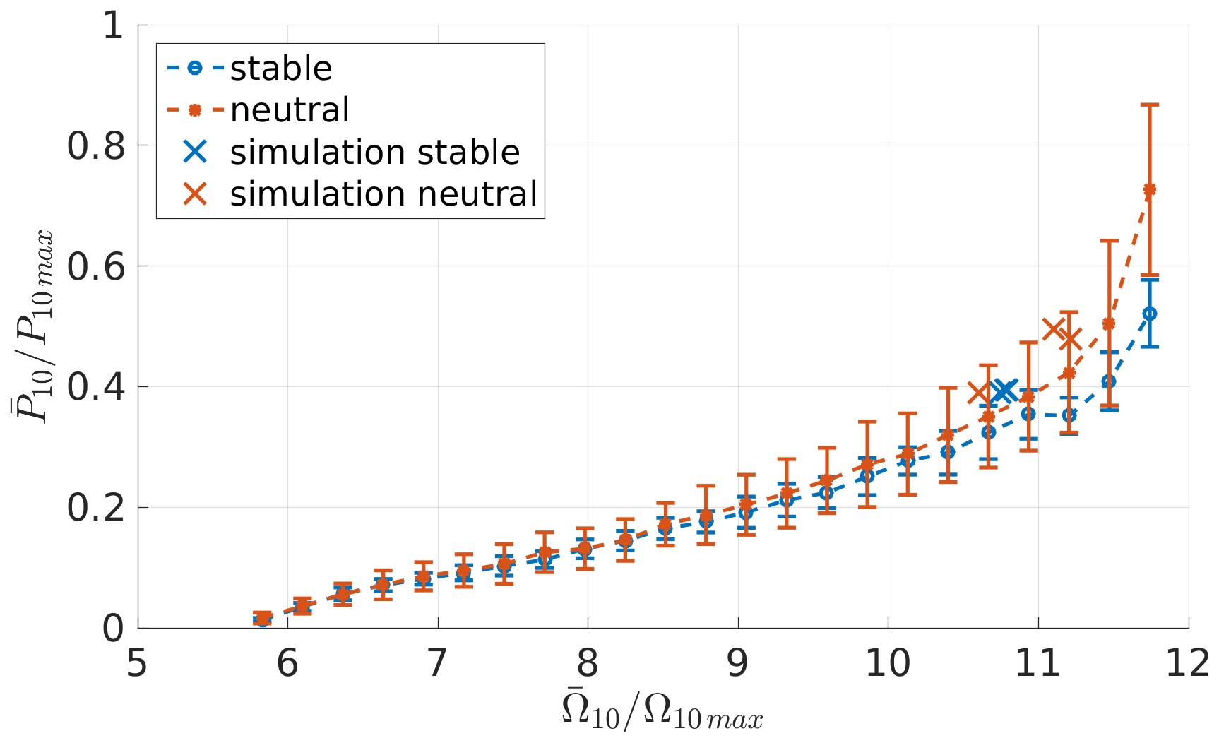
Figure 19 Power output normalised by the maximum measured power, plotted with respect to the rotor speed, and normalised with the maximum measured rotor speed with an added offset for the measurement data in comparison to the simulation data.

The values can be linked to the power spectra shown in Fig. 18. Particularly in the range of the lower frequencies larger power spectral density (PSD) values are obtained for the neutral case in comparison with the stable case. To investigate the influence of the lower frequencies on the equivalent load range, the equivalent load range for the tower top fore–aft bending moment is calculated with a high-pass filter as an example. The following values result for the equivalent load range when the frequencies below 0.1 are disregarded (stable: ${\mathrm{\Delta }}_{\mathrm{eq}}=\mathrm{81.8}\times {\mathrm{10}}^{\mathrm{5}}$kNm; neutral: ${\mathrm{\Delta }}_{\mathrm{eq}}=\mathrm{98.7}\times {\mathrm{10}}^{\mathrm{5}}$kNm), which clearly shows that the lower frequency range has a great influence on the equivalent load range. A higher value for the neutral case is expected as the flow contains larger eddies than the stable case.

This should be considered as a qualitative result. For a final quantitative analysis simulations with considerably larger run times or a number of simulations with different seeding would be required. Also, in the papers Lee et al. (2012) and Holtslag et al. (2016) no clear results are visible; in Lee et al. (2012) it is stated that mainly the roughness has an influence on the loads, while the stability has only a small effect. In Holtslag et al. (2016), on the other hand, a clear influence of stability on the loads is observed.

Table 7 Comparison of the equivalent load range Δ_eq of the simulation results (10 min interval), according to Eq. (3) with m=10 for blade loads and m=4 for tower loads.

As can be found in Fig. 19 the measurement data show a dependency on the atmospheric stability. Neutral conditions lead to higher power output for the same rotor speed than stable conditions. This behaviour might be explained due to the higher fluctuations caused by higher TI and the therefore higher energy content in the wind. However, the simulations did not reproduce the same dependency, which might be explained by the limited variability of the TI in comparison to the measurement data. As can be seen in Fig. 13 the simulations cover the lower limit of the TI in the respective wind speed.

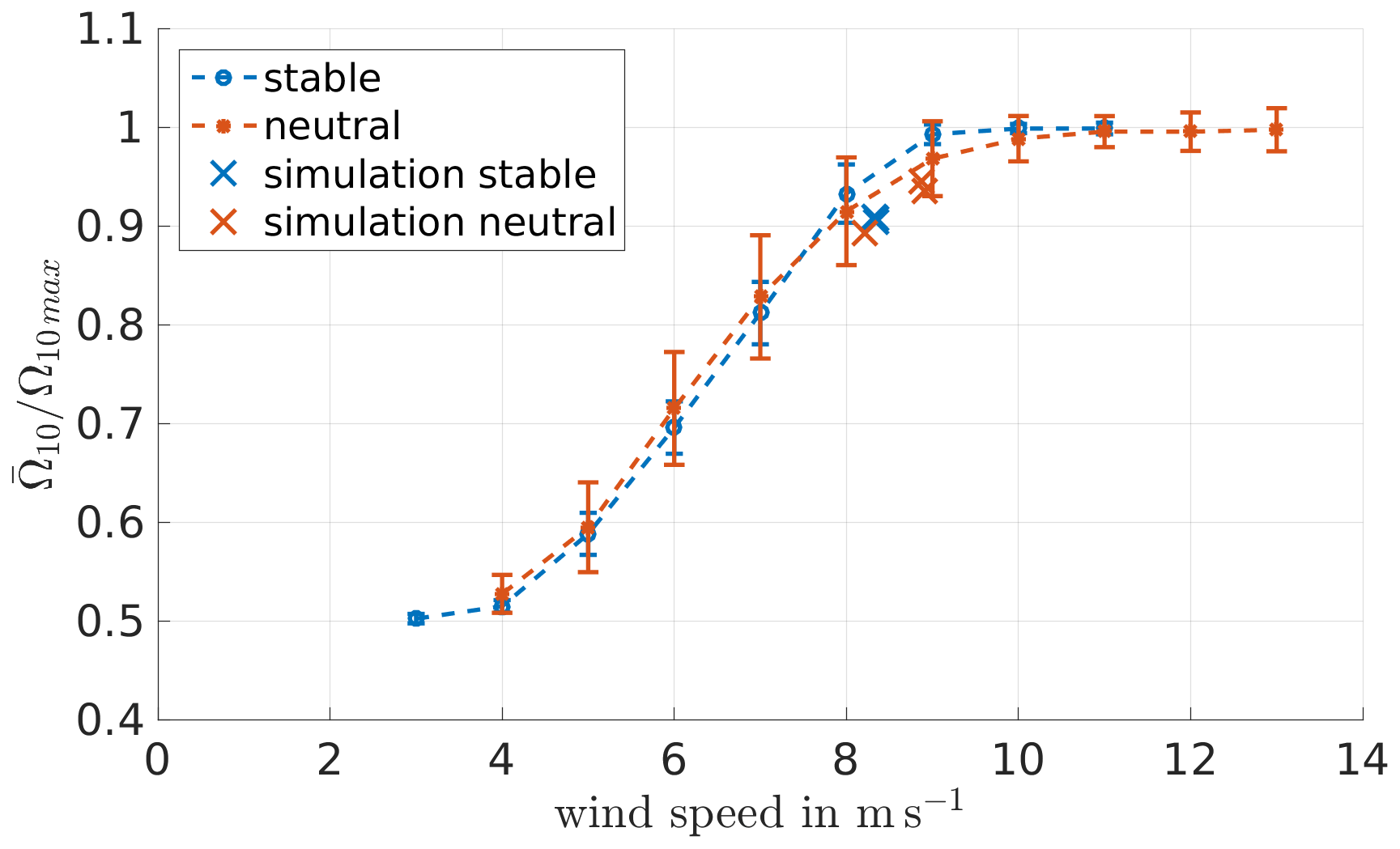
Figure 20 Relation between the rotor speed Ω, normalised with the maximum measured rotor speed with an added offset, with respect to the wind speed determined using the measurement data in comparison to the simulation data (×).

4 Conclusions

In this paper we presented a new computing framework which combines the advantages of an atmospheric flow simulation using the LES tool PALM and the detailed calculation of the turbine response by FAST. To quantify the output of the results a comparison to the generic NREL 5 MW turbine and a more extensive comparison to measurement data of a real turbine are shown.

The comparison of the NREL 5 MW turbine was intended to compare different model approaches with respect to power output and computing time. These showed very good agreement in terms of power output. Additionally, in the considered cases a saving of computational time of up to 89 % could be observed in relation to the equally detailed ALM coupling.

In a second step, the enhanced coupling was compared to measurement data. The results resemble the measured data of the eno114 3.5 MW turbine well. For example the power output is reproduced very well, which is mostly due to the method of taking the wind speed in front of the turbine instead of directly at the rotor area to avoid an overestimation of the power. Also, the standard variation of the power shows a good resemblance to the measurement data. The parameter reflects the influence of the turbulence in the flow and therefore the stability, which is also present in the simulated results. Keeping in mind that the simulations were still idealised, i.e. only one homogeneous roughness length and no topography, there is good agreement between the simulated and the measured data.

The blade and tower loads are representative of the measurements in general. Deviations in the aeroelastic simulation model, especially the tower eigenfrequency, the selected rotor imbalance, the used controller and wind speeds led to slightly different resulting loads compared to the measurements. However, the load spectra still show a very good agreement. Variations due to the atmospheric stability are clearly found. This indicates that the PALM–FAST coupling is suitable to investigate the effects of different atmospheric flows on turbine behaviour.

In the current work, the constraints of the frozen wind field, e.g. the assumption of Taylor’s frozen turbulence hypothesis, do not limit the outcome, as in the current simulations the statistics of the flow are not subject to varying wind conditions. However, there are also situations where the hypothesis will reach its limits, e.g. with temporally variable wind fields or changing wind direction. The case of a turbine in a wake also needs further investigation, as the recovery of the wake in the frozen wind field has not been considered so far. Therefore, for future work, a further comparison to measurement data of different situations, such as unstable stratification or in a turbine wake, is worth considering to further substantiate the results. However, due to the reduced computing time, the coupling is basically well suited for carrying out load analyses of a single turbine in a wind farm. As up to now ADM or ADMR has mostly been used in wind farms, since the use of ALM is too computationally intensive due to the required large model domains.

In addition, thanks to the time-saving detailed simulations, there is a multitude of possible applications. Apart from calculating load analyses for wind farms, another possible application is to investigate the relationship between environment and turbine performance in footprint analyses. Furthermore, phenomena in atmospheric flows and their impact on turbine loads can be investigated, such as low-level jets.

Appendix A: Blade elements in the NREL 5 MW turbine laminar case

The following plots show the dynamic pressure, the angle of attack, and the lift and drag coefficients for the NREL 5 MW turbine in the laminar case.

Figure A1 Dynamic pressure (a) and angle of attack (b) along the blade nodes in the laminar case of the NREL 5 MW turbine.

Figure A2 Lift (a) and drag (b) coefficient along the blade nodes in the laminar case of the NREL 5 MW turbine.

Appendix B: Spectra of the loads for the neutral case

The following plots show the blade and tower load spectra for the neutral case.

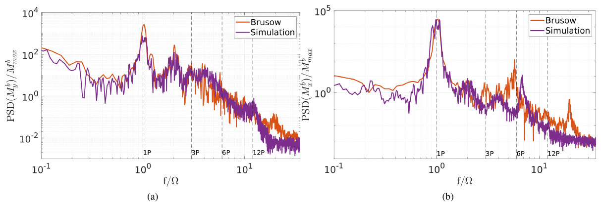
Figure B1 Spectrum of the blade root bending moment (a) out of plane $M_y^{\mathrm{b}}$ and (b) in plane $M_x^{\mathrm{b}}$ in comparison to the simulation results (neutral). The data are normalised by the maximum value of the blade root bending moments, and the frequency is normalised by the rotor speed.

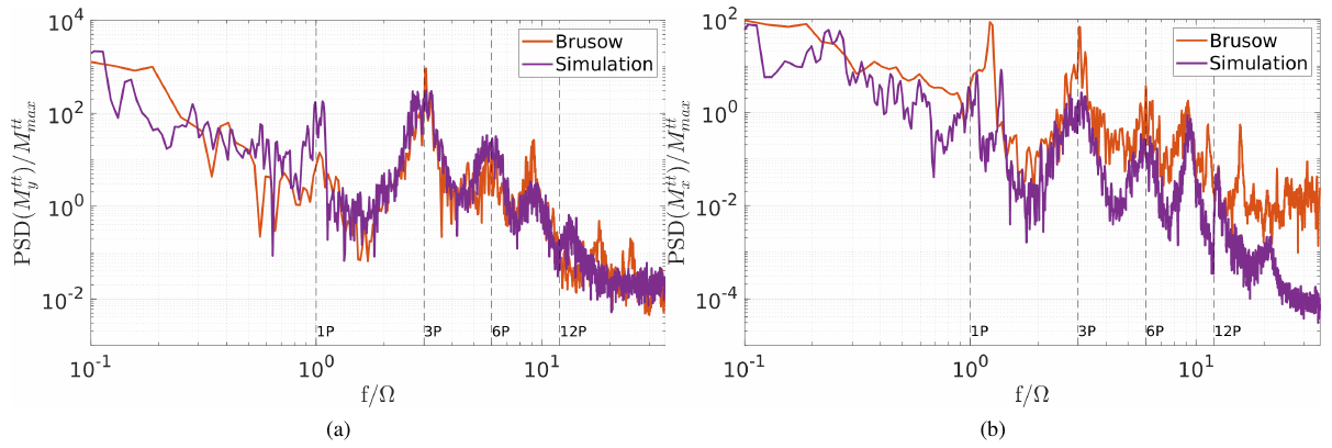
Figure B2 Spectrum of the tower top bending moment in (a) the fore-to-aft direction $M_y^{\mathrm{tt}}$ and (b) the side-to-side direction $M_x^{\mathrm{tt}}$; comparison of the measurement data to the simulation results (neutral). The data are normalised by the maximum value of the tower base bending moments, and the frequency is normalised by the rotor speed.

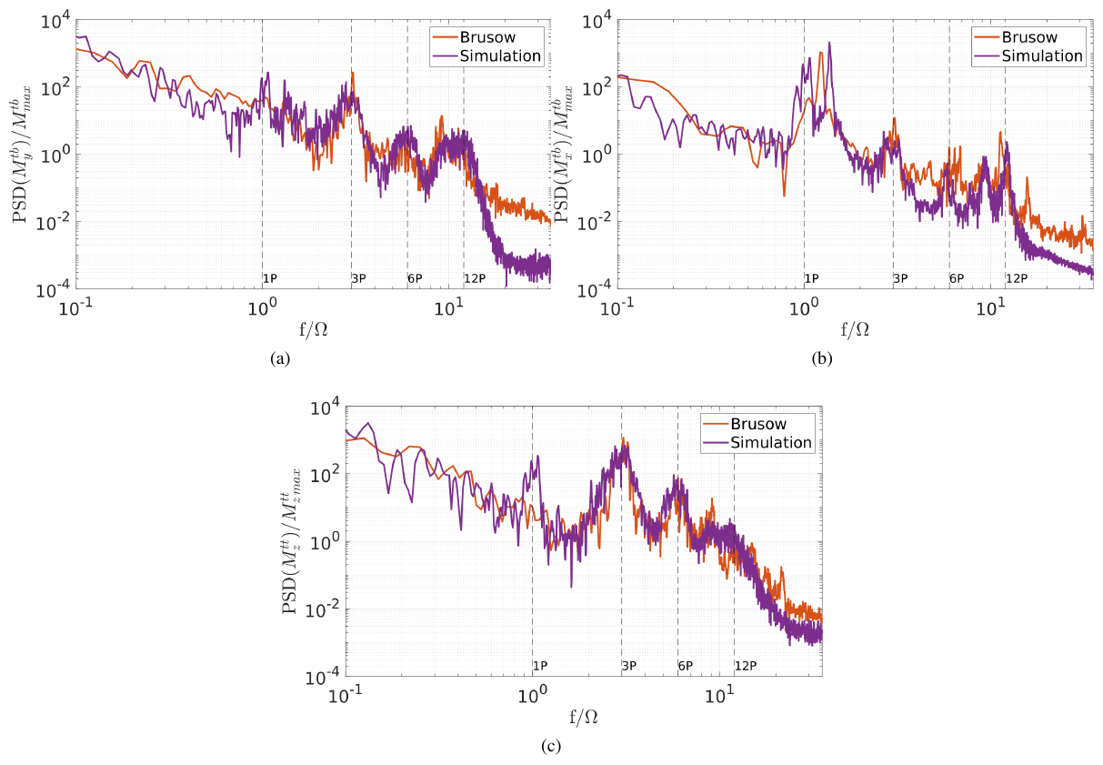
Figure B3 Spectrum of the tower moments: (a) the tower base bending moment in the fore-to-aft direction $M_y^{\mathrm{tb}}$, (b) the tower base bending moment in the side-to-side direction $M_x^{\mathrm{tb}}$ and (c) the tower top torsion moment $M_z^{\mathrm{tt}}$; comparison of the measurement data to the simulation results (neutral). The data are normalised by the maximum value of the tower top torsion moment, and the frequency is normalised by the rotor speed.

Appendix C: Wind profile comparison for the stable case

Here, the comparison of the wind profiles for the stable case is shown.

Figure C1 Wind profiles, calculated by the shear and wind speed, of the measurement interval and the simulation data used in the comparison of the loads for the stable case. The black lines indicate the rotor area, and the dashed line indicates the hub height.