Meso- to microscale modeling of atmospheric stability effects on wind turbine wake behavior in complex terrain

Terrain-induced flow phenomena modulate wind turbine performance and wake behavior in ways that are not adequately accounted for in typical wind turbine wake and wind plant design models. In this work, we simulate flow over two parallel ridges with a wind turbine on one of the ridges, focusing on conditions observed during the Perdigão field campaign in 2017. Two case studies are selected to be representative of typical flow conditions at the site, including the effects of atmospheric stability: a stable case where a mountain wave occurs (as in ∼ 50 % of the nights observed) and a convective case where a recirculation zone forms in the lee of the ridge with the turbine (as occurred over 50 % of the time with upstream winds normal to the ridgeline). We use the Weather Research and Forecasting Model (WRF), dynamically downscaled from the mesoscale (6.75 km resolution) to microscale large-eddy simulation (LES) at 10 m resolution, where a generalized actuator disk (GAD) wind turbine parameterization is used to simulate turbine wakes. We compare the WRF–LES–GAD model results to data from meteorological towers, lidars, and a tethered lifting system, showing good qualitative and quantitative agreement for both case studies. Significantly, the wind turbine wake shows different amounts of vertical deflection from the terrain and persistence downstream in the two stability regimes. In the stable case, the wake follows the terrain along with the mountain wave and deflects downwards by nearly 100 m below hub height at four rotor diameters downstream. In the convective case, the wake deflects above the recirculation zone over 40 m above hub height at the same downstream distance. Overall, the WRF–LES–GAD model is able to capture the observed behavior of the wind turbine wakes, demonstrating the model's ability to represent wakes over complex terrain for two distinct and representative atmospheric stability classes, and, potentially, to improve wind turbine siting and operation in hilly landscapes.

1 Introduction

Wind turbines are commonly sited in complex terrain to take advantage of topographic flow enhancement, such as the acceleration of flow over ridge lines and hill tops. In addition to topographic acceleration, other terrain-induced flow phenomena in the atmospheric boundary layer (ABL) affect wind turbine performance and wake propagation and characteristics (Xia et al., 2021; Draxl et al., 2021). These microscale processes include mountain/lee waves (and associated rotors), hydraulic jumps, valley flows, and flow separation and recirculation (Fernando et al., 2019; Baines, 1998).

The dynamics of terrain-induced flow phenomena vary based on the time of the day, with lee waves only occurring during stably stratified conditions, typical at night, and flow separation or recirculation often occurring during daytime convective (or unstably stratified) conditions. Interactions of the terrain with different stability conditions thus impact both the background flow and the resulting turbine performance. The difficulty of capturing the interaction between wind turbine wakes and complex terrain has historically limited research studies to wind tunnel experiments and numerical simulations with simple Gaussian and sinusoidal hills (see Porté-Agel et al., 2020, for a recent review on wind farm flows and topography). Additionally, turbine wake models used for designing wind farms typically do not account for terrain-induced flow phenomena and their effects on turbine wake behavior. Increased knowledge of wind flows in complex terrain is therefore critical to improve predictions to support growing wind energy resources (Veers et al., 2019).

In the present work, we use large-eddy simulation (LES) to examine the wake behavior of a wind turbine situated in complex terrain. LES explicitly solves for the most energetic eddies while parameterizing the effects of the smaller turbulent length scales on the resolved-scale flow. LES can therefore capture transient turbulent flow structures, which are important features of the ABL that interact with turbine wakes. While LES is computationally expensive, and thus requires the use of substantial high-performance computing resources, LES is increasingly complementing and in some cases replacing lower-fidelity techniques as a means to investigate wind turbine wake effects (see Stevens and Meneveau, 2017, for a recent review). Specifically, we utilize the LES capability of the Weather Research and Forecasting Model (WRF) (Skamarock et al., 2008; Powers et al., 2017) for our simulations.

The multi-scale framework in WRF dynamically downscales mesoscale forcing to microscale LES using a grid nesting approach, with lateral boundary conditions provided from each parent domain. Such setups can provide LES with realistic time-varying inflow conditions directly from the mesoscale simulations.

Implementation of a wind turbine actuator disk parameterization within the nested LES domain provides a unique turbulence-resolving simulation framework for wind turbine wake prediction in turbulent flow settings under more realistic environmental and atmospheric forcing conditions. This study utilizes a generalized actuator disk (GAD) wind turbine parameterization on the finest domain following Mirocha et al. (2014) and Wu and Porté-Agel (2011). In the GAD parameterization, thrust and rotational forces computed at the turbine's blades are averaged over a discretized two-dimensional disk formed by their rotation. These forces are then applied to the flow surrounding the turbine, capturing both the velocity deficit and rotation of the wake, which simpler parameterizations (such as the Fitch et al., 2013, wind farm parameterization) neglect. The GAD tool has been previously validated and shown to capture turbine–airflow interactions and wake behavior at grid resolutions of 10 m in simple terrain (Mirocha et al., 2015; Aitken et al., 2014; Marjanovic et al., 2017; Arthur et al., 2020). However, the multi-scale WRF–LES–GAD framework (hereinafter used to denote the model in its entirety) has yet to be evaluated in complex terrain where the combination of terrain and thermal stratification directly affects the flow and impacts operating turbines.

The test location chosen in this study is that of the Perdigão field campaign (Fernando et al., 2019), which took place in 2017 in Portugal. The Perdigão experiment characterized the flow over two parallel ridges with a wind turbine located on the southwest ridge and provided valuable data for characterizing wind turbine wakes in complex terrain (Menke et al., 2018; Barthelmie and Pryor, 2019; Wildmann et al., 2018, 2019). Menke et al. (2018) classified wind turbine wake behavior based on atmospheric stability using scanning Doppler lidars at Perdigão, identifying four different cases based on the stratification: a “stable + mountain wave” case where the wake deflected downwards following the terrain, “stable” and “neutral” cases where the wake remained at a constant height above sea level, and “unstable” cases where the wake deflected upwards. Barthelmie and Pryor (2019) similarly characterized wake behavior at Perdigão based on atmospheric stability. Using measurements averaged over longer time periods (10 min compared to 24 s in Menke et al., 2018), they inferred that all wakes were initially lofted and then strongly influenced by stability, with wake centers moving downwards in unstable conditions and also generally moving downwards but remaining at greater heights during stable conditions. The different findings in these two studies motivate the need to further study wind turbine wakes in complex terrain.

Two fine-scale (Δx = 10 m) LES modeling studies of the Perdigão campaign have been conducted with a wind turbine parameterization, both in idealized conditions with neutral stability. Berg et al. (2017) performed idealized LES of the Perdigão site in neutral atmospheric stability conditions and showed that the steep terrain in Perdigão resulted in the formation of a recirculation zone with which the wake did not interact. Instead, the wake advected at a constant height above sea level like the neutral case characterized by Menke et al. (2018). Dar et al. (2019) also simulated the Perdigão site using idealized LES to examine the self-similarity of wind turbine wake behavior as a function of varying terrain complexity under neutral stratification. They found that self-similarity is preserved for a shorter distance compared to what is observed in flat terrain and that the wake propagation was similar to that seen by Berg et al. (2017). There have also been two relatively coarse nested LES studies of the Perdigão campaign by Connolly et al. (2021) and Wagner et al. (2019), where grid resolutions of 150 and 200 m were used, respectively, with both utilizing the LES capability of WRF. The findings from these studies have provided guidance for the setup used in this study (as discussed in Sect. 3), but their setups are too coarse to resolve a utility-scale wind turbine with a rotor diameter of 80 m.

The goal of this work is to examine the ability of the WRF–LES–GAD framework to capture terrain-induced flows and their interaction with an operating wind turbine at the Perdigão site (described further in Sect. 2), to thereby demonstrate the efficacy of mesoscale-to-microscale coupled simulations to improve wind plant simulations in complex terrain. We focus on two distinct but representative case studies with different atmospheric stability regimes, convective and stable, both of which were commonly observed during the field experiment. We validate the predicted flow structure and turbine wake behavior during each case study using comparisons with observations from meteorological towers, scanning lidars, and a tethered lifting system (Sect. 4). Furthermore, we present a detailed analysis of the turbine wake in both stability regimes in order to comment on the discrepancy in the observational studies discussed above.

2 Case study

2.1 Overview of the Perdigão campaign

The Perdigão field campaign was a European Union–United States collaboration of over 70 scientists, engineers, and support personnel. The Perdigão site, named for a village located near the Vale do Cobrão in eastern Portugal, consists of two parallel ridges with a 2 MW (megawatt) wind turbine located on the southwest ridge (see Fig. 1). This site was selected because the straight valley extends over 2 km in distance, suggesting that the flow could be representative of an idealized two-dimensional valley flow in nature. Additionally, the annual climatology showed that common wind directions measured at ridge top are perpendicular to the ridges (Fernando et al., 2019).

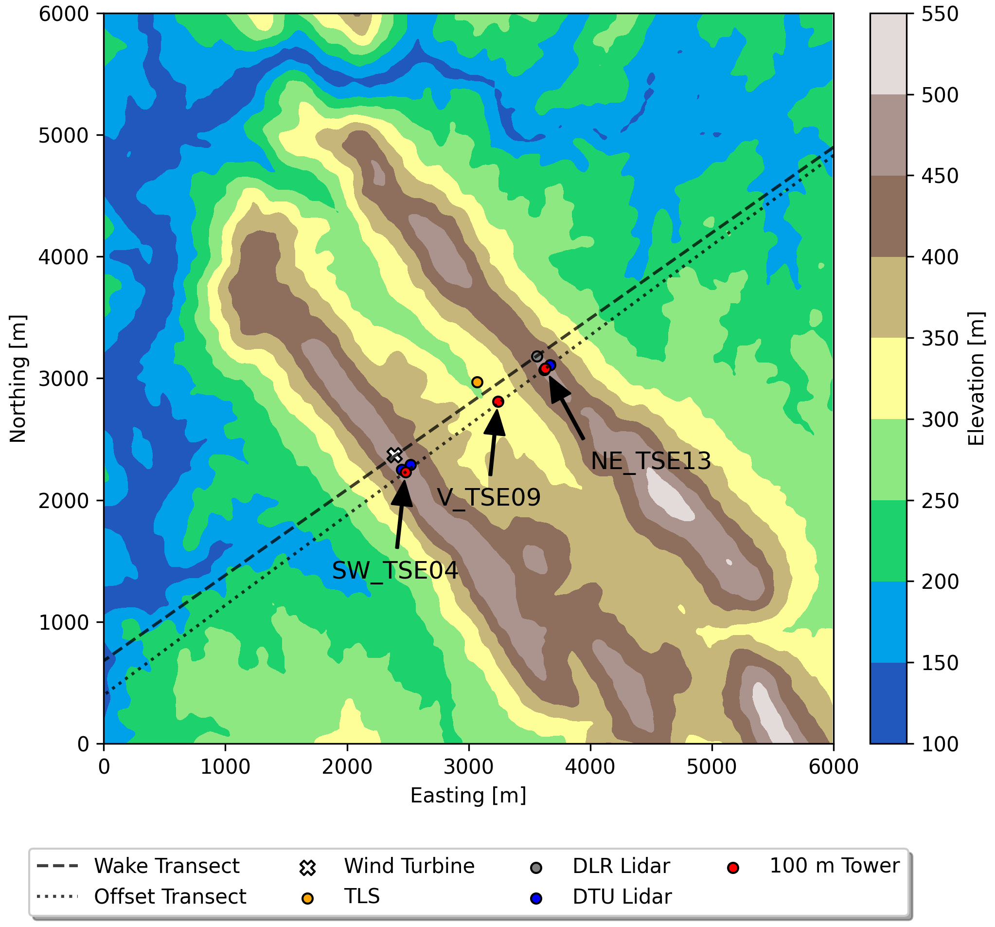
Figure 1 Terrain and layout of the Perdigão site showing the location of relevant instrumentation. The wake and offset transects are used for analysis later in this paper. Each of the three 100 m meteorological towers is labeled following the naming convention in the publicly available dataset corresponding to their geographic location.

During the intensive operation period from 1 May 2017 to 15 June 2017, a comprehensive, high-resolution dataset was collected. Instrumentation included 100 m meteorological towers (hereinafter referred to as met towers), lidars, a tethered lifting system (TLS), and numerous shorter meteorological towers and radiometers. The instrumentation of interest is discussed here, and the layout of the Perdigão field site is shown in Fig. 1.

Three 100 m met towers were placed along a transect roughly perpendicular to the ridges (see Fig. 1). SW_TSE04, located approximately 150 m southeast of the wind turbine laterally along the ridgeline, is representative of inflow conditions. V_TSE09 is located in the valley, and NE_TSE13 is on the northeast ridge. These three towers have booms angled at 135^∘ from north located at heights of 10, 20, 40, 60, 80, and 100 m with sonic anemometers sampling three-dimensional velocity at 20 Hz. In this paper, data representative of near-surface winds (10 m) and at hub height (80 m) are examined. Temperature sensors available at 10 and 100 m are used to characterize atmospheric stability using a simple temperature gradient similar to Menke et al. (2019).

A tethered lifting system (TLS) from the University of Colorado, Boulder, was also launched from the valley. The TLS is a unique device that is able to obtain in situ measurements of wind speed, wind direction, and temperature aloft at 1 kHz (Balsley, 2008). GPS measurements of latitude, longitude, and altitude are sampled at 5 s. When in profiling mode, the TLS ascends and descends at ∼ 0.3 m s⁻¹ and covers a vertical range of ∼ 400 m. The capabilities of the TLS have been demonstrated in several field campaigns, including a previous wind turbine wake investigation (Lundquist and Bariteau, 2015).

Simulation results are also compared with scanning Doppler lidar data. The first is a scanning lidar operated by the German Aerospace Center (DLR) located on the northeast ridge (Wildmann et al., 2018). This lidar's scanning trajectory is perpendicular to the wind turbine rotor allowing for the wake to be captured in addition to relevant flow features in the valley. The second set of scanning lidars used here were operated by the Technical University of Denmark (DTU) (Menke et al., 2020). Four lidars, two on each ridge, scanned a transect perpendicular to the valley. Because of how the lidars are arranged, a multi-Doppler lidar scan of the valley, the two ridges, and the surrounding area can be formed. This multi-Doppler lidar scan does not capture the wind turbine wake but does show microscale features that interact with the wind turbine wake (as seen later in Fig. 4).

2.2 Case studies and phenomena of interest

Two terrain-induced flow features characteristic of the field site are of interest for the present work: (a) mountain waves and (b) recirculation zones, which occur frequently at the Perdigão site depending on the time of day (Menke et al., 2019; Fernando et al., 2019; Wagner et al., 2019). Fernando et al. (2019) found that mountain waves occurred for almost 50 % of the nights during the intensive operation period, while Menke et al. (2019) found that recirculation occurred over 50 % of the time when the wind direction was perpendicular to the ridges. To help select appropriate time periods representing mountain waves and recirculation zones, we examine a few stability parameters.

Mountain waves can occur when stably stratified flow approaches a topographic disturbance, such as a mountain ridge. These waves can be described using a ratio of inertial to buoyant forces represented by the internal Froude number (Stull, 1988),

$$\begin{array}{}\text{(1)}& \mathit{Fr}={\displaystyle \frac{\mathit{\pi }U}{WN}},\end{array}$$

where W is the mountain ridge width (defined for the southwest ridge of Perdigão to be 586.5 m on average according to Palma et al., 2020), U is the free-stream wind speed, and N is the Brunt–Väisälä frequency, defined as

$$\begin{array}{}\text{(2)}& N=\sqrt{{\displaystyle \frac{g}{\mathit{\theta }}}{\displaystyle \frac{\partial \mathit{\theta }}{\partial z}}}.\end{array}$$

Here g is the gravitational constant, θ is the potential temperature of the environment, and $\frac{\partial \mathit{\theta }}{\partial z}$ is the lapse rate or vertical gradient in potential temperature. The internal Froude number can also be defined as the ratio of the natural wavelength of the air ($\mathit{\lambda }=\mathrm{2}\mathit{\pi }U{N}^{-\mathrm{1}}$) to the effective wavelength of the mountain ridge (2W).

For subcritical flow (Fr<1), when wind speeds are low or the stability is very strong, λ is much shorter than 2W, resulting in weak mountain waves. Mountain waves resonate when Fr∼1, resulting in strong updrafts and downdrafts where rotors (and potentially hydraulic jumps) are present (Jackson et al., 2013). When wind speeds are strong and stability is weak, Fr>1 and flow is supercritical, resulting in long wavelengths with the potential for reverse flow in the lee of the mountain.

Neutral and convective conditions represent the theoretical case of Fr∼∞, when a turbulent mountain wake with recirculation forms instead of mountain waves. Relevant to this study are Fr≈1 during stable conditions and Fr≈∞ during convective conditions. For more information regarding mountain waves, the reader is referred to Stull (1988), Baines (1998), and Jackson et al. (2013).

Quantifying atmospheric stability in complex terrain is an active research area. Using a gradient Richardson number is difficult because of the effect of terrain-induced flow speedup over the ridge affecting the shear terms (Menke et al., 2019). Bodini et al. (2020) calculated the Obukhov length for Perdigão and found that it was not very powerful in predicting dissipation rate. Despite this, the Obukhov length is still useful for selecting stable and unstable case studies. The Obukhov length, L, is defined as

$$\begin{array}{}\text{(3)}& L={\displaystyle \frac{-u_{\ast }^{\mathrm{3}}\mathit{\theta }}{\mathit{\kappa }g\stackrel{\mathrm{‾}}{w^{\prime }{\mathit{\theta }}^{\prime }}}},\end{array}$$

where u_∗ is the friction velocity, κ is the von Kármán constant (taken as 0.4), w is the vertical velocity, and $w^{\prime }{\mathit{\theta }}^{\prime }$ is the surface heat flux. The prime denotes fluctuations and the overbar a mean. The friction velocity is defined as

$$\begin{array}{}\text{(4)}& u_{\ast }={\left({\stackrel{\mathrm{‾}}{u^{\prime }{w}^{\prime }}}^{\mathrm{2}}+{\stackrel{\mathrm{‾}}{v^{\prime }{w}^{\prime }}}^{\mathrm{2}}\right)}^{\mathrm{1}/\mathrm{4}}.\end{array}$$

The Obukhov length and friction velocity, valid for the surface layer, are calculated at SW_TSE04 using 5 min statistics from the lowest sensors available at 10 m. Obukhov lengths between 0 and 500 m are considered stable and 0 to −500 m unstable.

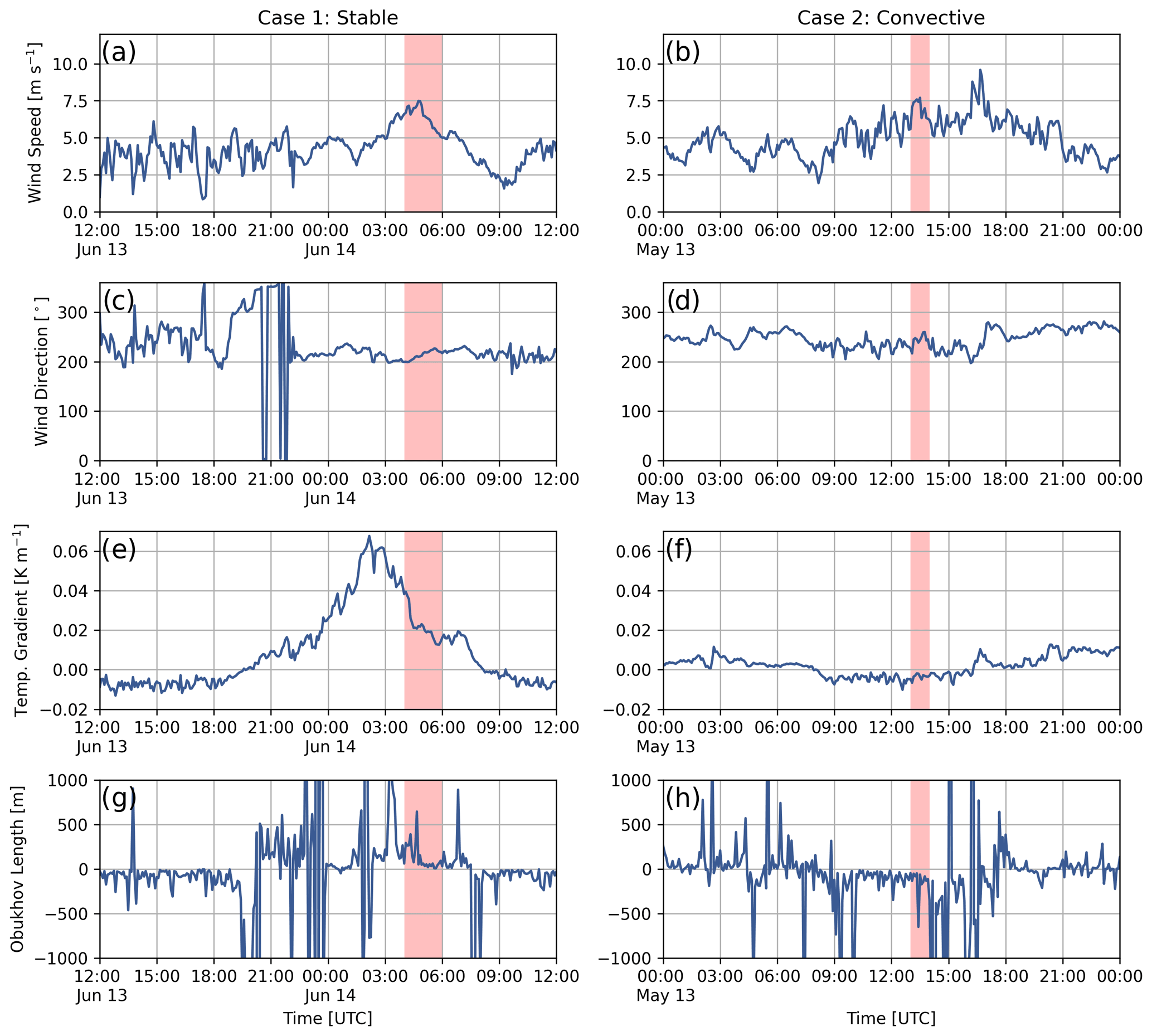
Figure 2 Hub-height (80 m) wind speed, wind direction, 100–10 m potential temperature gradient, and Obukhov length for the stable case and for the convective case. Data are from SW_TSE04, and the periods of interest are highlighted in red. Data have been subsampled to 5 min intervals.

In addition to the Obukhov length, the potential temperature gradient between 10 and 100 m at SW_TSE04 is used as a proxy for atmospheric stability throughout this study and when comparing observations with the model. Note that SW_TSE04 was not outfitted with any pressure sensors; therefore, the potential temperature is approximated by $\mathit{\theta }\approx T+(g/C_p)\cdot z$, where $(g/C_p)$ = 0.0098 K m⁻¹ as was done by Menke et al. (2019). Figure 2 shows wind speed, direction, temperature gradient, and Obukhov length for two different dates during the field campaign, and representative time periods are selected from these for the stable and convective case studies. The met tower measured periods of counter-gradient heat fluxes during both stable and convective conditions but not during the time periods selected for this tower location.

2.2.1 Case 1: stable conditions

The early morning of 14 June 2017 shows typical stably stratified conditions as indicated by a positive temperature gradient and Obukhov length in Fig. 2e and g, respectively. From 04:00 to 06:00 UTC (05:00 to 07:00 LT, local time, with sunrise at 06:02 LT), the hub-height wind direction is relatively constant between 200 and 220^∘ (Fig. 2c). These wind directions are close to a southwesterly wind of 215^∘, perpendicular to the ridges. The average wind speed is 6.3 m s⁻¹, a speed in which the turbine will operate and generate wake effects. Using the average wind speed (6.3 m s⁻¹), temperature gradient or lapse rate (0.031 K m⁻¹), potential temperature of the environment (296.7 K), and width of the southwestern ridge of Perdigão (586.5 m), the average internal Froude number during the period of interest is calculated to be 1.05. With a Froude number close to one, we expect a resonant mountain wave to occur.

2.2.2 Case 2: convective conditions

Typical daytime convective conditions on 13 May 2017 are indicated by the negative temperature gradient and Obukhov length in Fig. 2f and h, respectively. For much of the day (08:00–16:00 UTC, 09:00–17:00 LT), the temperature gradient is approximately −0.005 K m⁻¹. During the period of interest (13:00–14:00 UTC) a wind speed of 7 m s⁻¹ causes the wind turbine to operate and generate wake effects. The negative lapse rate results in an infinite internal Froude number, and with wind perpendicular to the ridge a turbulent mountain wake with recirculation should form.

3 Methods

3.1 WRF–LES–GAD

The present work utilizes the large-eddy simulation capability of the WRF model, version 3.7.1, with modifications including vertical grid nesting (Daniels et al., 2016), the generalized actuator disk (GAD) (Mirocha et al., 2014), and a turbine yawing capability (Arthur et al., 2020). The GAD requires specifications for the turbine's airfoil lift and drag coefficients. The turbine located at the Perdigão site is a 2.0 MW E-82 Enercon turbine; however, the required lift and drag parameters are not publicly available. We therefore use the wind turbine parameterization from Arthur et al. (2020), which is similar but not identical to the turbine at Perdigão. Both turbine types have a roughly 80 m hub height and rotor diameter and are therefore expected to create similar wake effects. Minor differences between the two turbines are not expected to be critical to the conclusions of this study.

Table 1 Parameters used for the nested multi-scale WRF–LES–GAD setup. For the vertical resolution, Δz_min is for the first grid point above the surface and is approximate due to the nature of the terrain-following coordinate system in WRF.

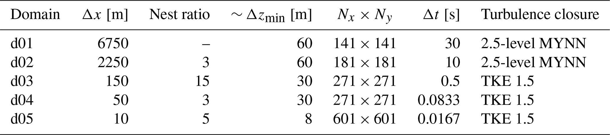
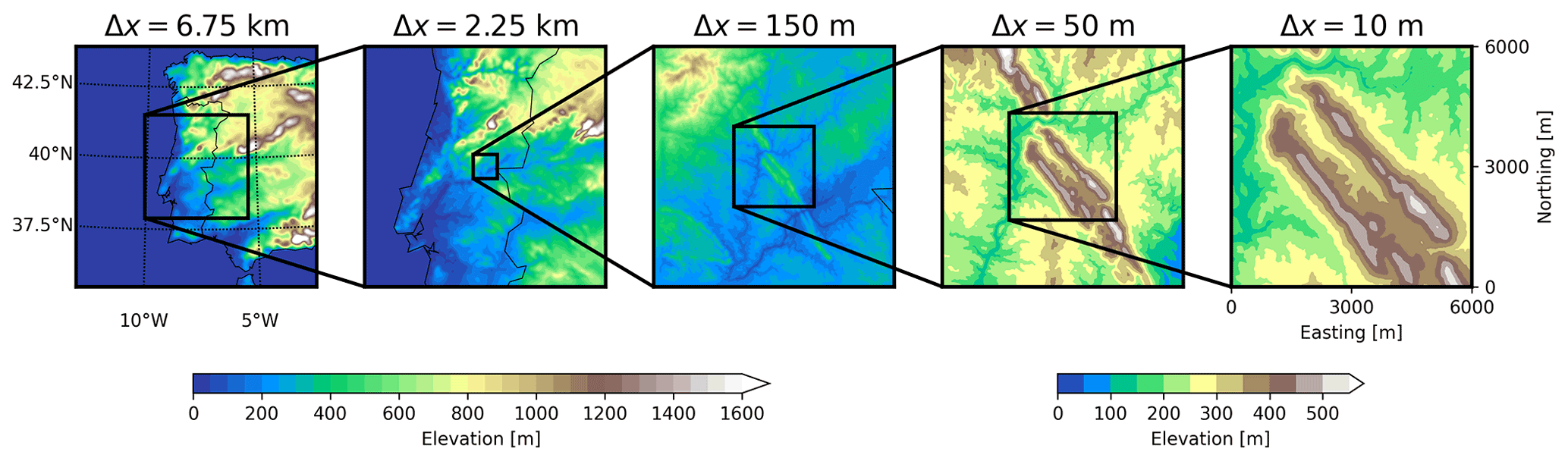
Figure 3 Topography of domains used in the multi-scale simulation centered over the Perdigão site. The five domains have resolutions of 6.75 km, 2.25 km, 150 m, 50 m, and 10 m. Dimensions of each domain and other configuration information are included in Table 1.

3.2 Multi-scale simulation setup

The five-domain nested multi-scale setup for WRF–LES–GAD is shown in Fig. 3, with details in Table 1. The outermost domain, d01, captures mesoscale forcing and has a horizontal grid resolution of 6.75 km; the innermost domain, d05, uses 10 m spacing and captures microscale flow features. The two coarsest domains are mesoscale simulations that use a planetary boundary layer (PBL) scheme, while the three inner domains use a microscale LES turbulence closure. There is a relatively large parent grid ratio of 15 from d02 to d03, intentionally chosen to skip across the gray zone where turbulence is only partially resolved (Wyngaard, 2004; Chow et al., 2019; Haupt et al., 2019; Muñoz-Esparza et al., 2017). The multi-scale setup also makes use of vertical grid nesting (Daniels et al., 2016) to adjust the vertical layers in each domain, with grid spacing as fine as 8 m near the surface for d05 and increasing for the coarser domains, up to roughly 60 m near the surface for d01. The coarser vertical resolution for d01–d04 has the benefit of reducing computational costs (the current setup takes roughly 8 h of wall-clock time for 5 min of simulation time on 288 cores) while also maintaining an aspect ratio ($\mathrm{\Delta }x/\mathrm{\Delta }z$) closer to unity on the LES domains d03 and d04 (Daniels et al., 2016). On d05, most of the vertical resolution is devoted to the bottom ∼ 2 km of the atmosphere, above which there is a gradual drop-off in resolution all the way to the domain top of ∼ 20 km. Because of the steepness of the terrain, numerical stability requires the use of very small time steps (as small as $\mathrm{1}/\mathrm{60}$ s for d05). Domains d01, d02, and d03 were spun up for 9 h, prior to starting d04 and d05.

All three LES domains (d03, d04, and d05) use a stochastic inflow perturbation method (the cell perturbation method; CPM) to improve the downscaling of coherent, turbulent structures in the nested approach (Muñoz-Esparza et al., 2014, 2015) in a range of stability conditions (Muñoz-Esparza and Kosović, 2018). The CPM works by applying small temperature perturbations to the flow on the upwind domain boundaries that accelerate the development of a full range of turbulent scales, at essentially no additional computational cost. While the use of high-resolution terrain data is expected to spur turbulence, Connolly et al. (2021) found that during convective conditions in the Perdigão valley, using the CPM further improved the representation of turbulence and the rate at which smaller-scale turbulence forms, with no known negative impacts on the flow from the perturbations. Similar findings regarding CPM are described by Arthur et al. (2020) for nested WRF–LES–GAD simulations of a wind farm in less complex terrain.

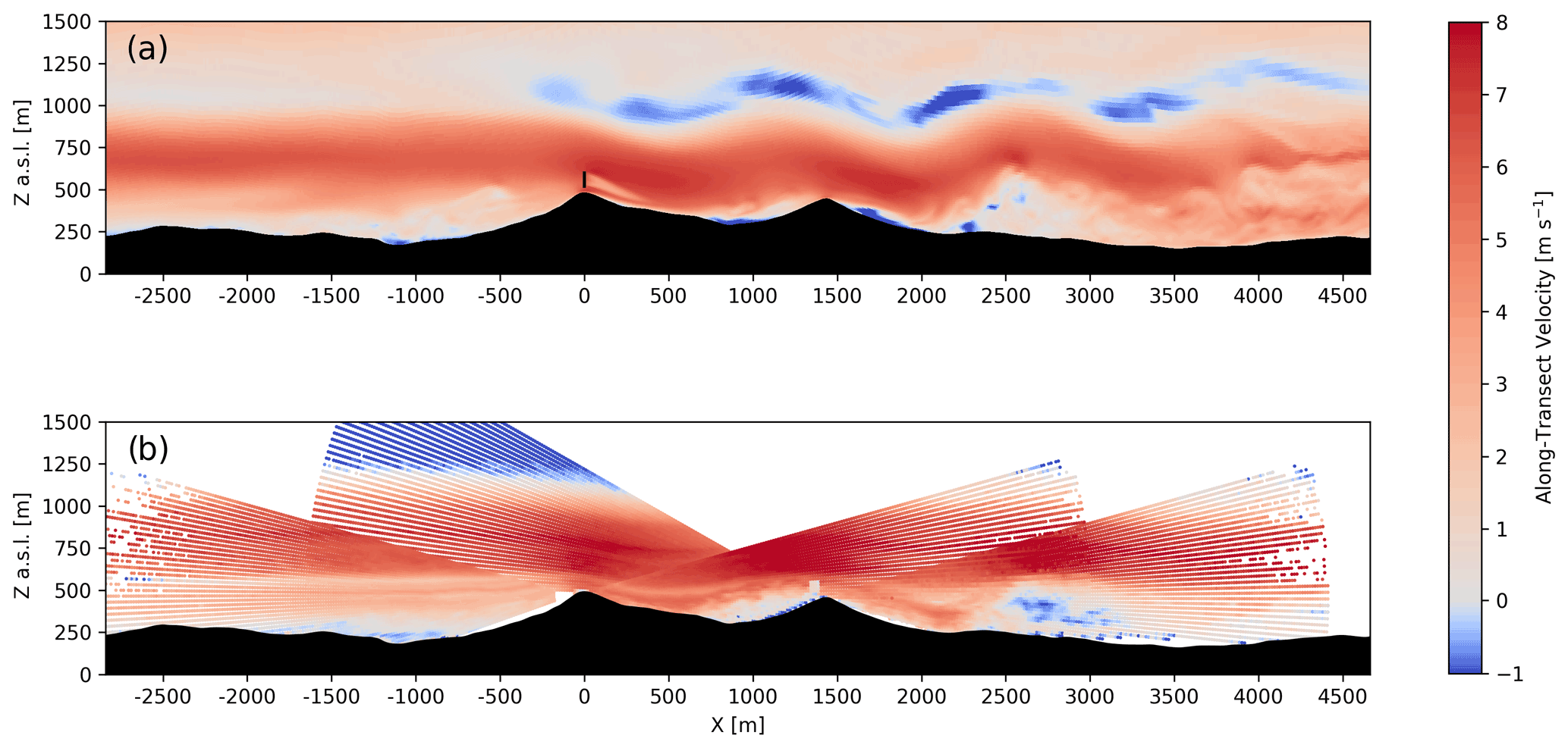
Figure 4 Instantaneous along-transect horizontal velocity during the stable case study for (a) the model and (b) the DTU multi-Doppler lidar scan at approximately 04:20 UTC. The output from the model is instantaneous while the multi-Doppler measurements are over the course of a single scan, which takes about 24 s. The model transects are aligned with the wake transect and the lidar transects are aligned with the offset transect in Fig. 1. An animation of model results during the entire 2 h period is included in the supplementary material (see Video 1 in the Video supplement).

WRF–LES–GAD is run using a third-order Runge–Kutta time advancement scheme, with fifth-order horizontal and third-order vertical advection schemes. Relevant physical parameterizations selected include the Eta (Ferrier) scheme for microphysics (Rogers et al., 2001), the Noah land surface model (Chen and Dudhia, 2001), the Rapid Radiative Transfer Model for longwave radiation (Mlawer et al., 1997), and the Dudhia shortwave radiation model (Dudhia, 1989). The mesoscale simulations, d01 and d02, use the Mellor–Yamada–Nakanishi–Niino (MYNN) level-2.5 PBL scheme (Nakanishi and Niino, 2006, 2009), and d03, d04, and d05 use the turbulent kinetic energy (TKE) level-1.5 LES closure (Deardorff, 1980). All domains use the MYNN surface layer scheme in which the lower-boundary conditions are determined from Monin–Obukhov similarity theory. Additionally, topographic shading is enabled to account for shading effects on the surface heat flux in the complex Perdigão terrain. For the upper-boundary condition, we use a Rayleigh damping layer for the top 5 km of the domain.

Mesoscale forcing for d01 is provided by Global Forecast System (GFS) data from the National Centers for Environmental Protection (National Centers for Environmental Prediction, National Weather Service, NOAA, U. S. Department of Commerce, 2015). In a sensitivity study comparing both GFS and European Centre for Medium-Range Weather Forecasts data for the boundary conditions, the GFS data produced more accurate results near the surface for the dates of interest here (Wendels, 2019).

Land cover data were obtained from the Coordination of Information on the Environment (CORINE) dataset at a resolution of 100 m, much finer than the default land cover data provided in WRF. The CORINE Land Cover 2006 raster dataset (Bossard et al., 2000) is transformed into United States Geological Survey (USGS) land use types to obtain surface roughness lengths for WRF (Pineda et al., 2004). The CORINE dataset seemingly misclassifies the land type in the valley as mixed shrubland/grassland when the vegetation is mostly tall eucalyptus and fir trees. Likewise, Wagner et al. (2019) concluded that the surface roughness lengths at the Perdigão site based on the CORINE land cover data were too small. To account for this, we set the surface roughness length for the mixed shrubland/grassland land use category in the valley to 0.5 m, the same value used in the LES studies of Berg et al. (2017) and Dar et al. (2019). High-resolution terrain data (1 arcsec, approximately 30 m) were obtained from the Shuttle Radar Topography Mission (Farr et al., 2007). These high-resolution terrain data are required to resolve flow features within the narrow valley (see Appendix A for more details).

Figure 5 Transect of 1 h time-averaged along-transect velocity for the (a) model and (b) DLR lidar during the stable case study with panel (c) as the difference between the DLR lidar and the model. The transects are aligned with the wake transect in Fig. 1.

4 Results and discussion

4.1 Validation of the stable case study

The stable case is influenced by a mountain wave event. To validate the accuracy of this event in WRF–LES–GAD, we compare the model with multi-Doppler lidar scans obtained by the DTU lidars. The model u and v velocities have been projected onto a rotated coordinate system aligned with the wake transect in Fig. 1 for comparison. For the lidar, the line-of-sight velocities have been converted into horizontal velocity along the offset transect in Fig. 1. Velocity components perpendicular to the lidar's line of sight are not captured, so this conversion results in larger errors at higher-elevation angles, but errors are small across the valley near the wind turbine, where the lidar beam is near horizontal. The wavelength of the mountain wave is defined as the distance from the first ridge (where the low-level jet begins to deform) to the first crest of the mountain wave. The model predicts a wavelength of 1220 m (Fig. 4a), 13 % less than the 1410 m wavelength from the DTU lidars, which is almost exactly the ridge-to-ridge distance of 1400 m (Palma et al., 2020). In both the model and multi-Doppler lidar scans, the flow follows the terrain over each ridge, creating a small rotor in the Perdigão valley and a larger rotor beneath the third wave crest downstream of the valley.

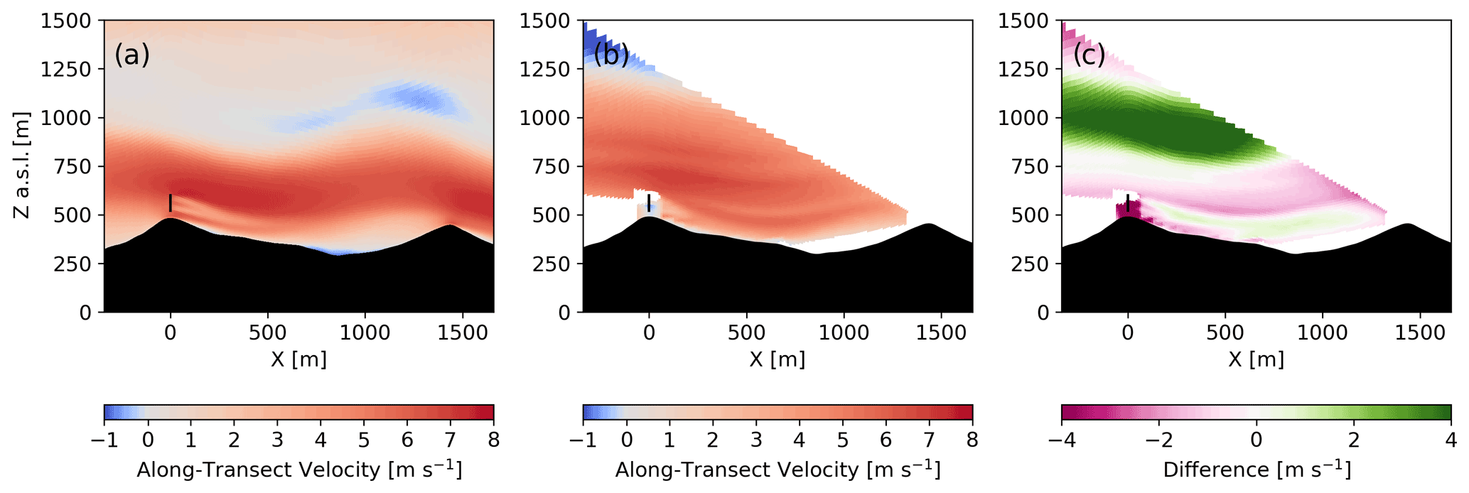
Figure 5 shows 1 h (from 04:30 to 05:30 UTC) time-averaged along-transect velocities for the stable case from the model and the DLR lidar scan along the wake transect (Fig. 1). The lidar data are interpolated onto the model grid, and the difference between the model and observations is shown in Fig. 5c. The height of the mountain wave does not extend as high in the model compared to measurements, likely a result of errors in the GFS forcing. This is clear in Fig. 5c, where there are large differences in the along-transect velocity from roughly 800–1200 $\mathrm{m}\mathrm{a}.\mathrm{s}.\mathrm{l}.$ The lidar data also show striations of slower and faster wind speeds within the wave, but these striations are not captured by the model. For both the model and the lidar scans, the wake propagates downward, following the terrain into the valley. The velocity deficit from the turbine wake dissipates more quickly in the observations compared to the model. The model's resolvable turbulent length scale is limited by the grid resolution, making it possible that the model turbulence dissipation is underpredicted; in addition, this could be due to the different turbine model or errors from a number of other parameterizations.

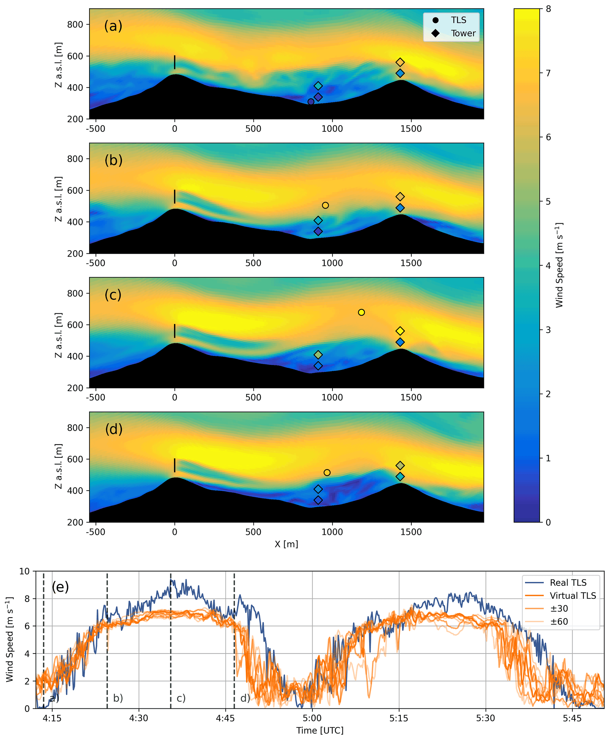
Figure 6 Transects of instantaneous wind speed for WRF with measurements from V_TSE09, NE_TSE13, and the TLS overlaid for (a) 04:13:30 UTC, (b) 04:24:30 UTC, (c) 04:35:30 UTC, and (d) 04:46:30 UTC and (e) comparison of wind speed between the TLS data and the virtual TLS in WRF–LES–GAD d05. The transects are aligned with the wake transect in Fig. 1. Virtual TLSs with an easting and northing position ± 30 and ± 60 m are shown with a lighter shading, and dashed lines indicate the times shown in the transects. An animation of model results for when the TLS is operational is included in the supplementary material (see Video 2 in the Video supplement).

Figure 6 shows instantaneous wind speed from the model overlaid with measurements from the TLS, as well as met towers V_TSE09 and NE_TSE13, at times when the TLS is near the surface, halfway up, near the top of its ascent, and halfway down its descent (the tower on the southwest ridge is omitted for clarity). Figure 6e shows a time series from the model, a virtual TLS, extracted using the GPS position at the corresponding time step of the actual TLS. Comparison of time-dependent turbulent flow fields from a model and a measurement system that moves in three dimensions over time is difficult because the instantaneous positioning of turbulent flow features will likely not match. To partially account for this and for any uncertainty of the TLS positioning (estimated to be ± 30 m), the wind fields in Fig. 6a–d have also been spatially averaged by ± 30 m in the spanwise direction. Additionally, time series with an easting and northing position ± 30 and ± 60 m are shown in Fig. 6e but with a lighter shading. During the two ascents, the virtual TLS and real TLS show good agreement with a root mean squared error (RMSE) under 2.0 m s⁻¹. However, the model slightly underestimates the strength of the jet, and there is a negative bias of −0.78 m s⁻¹ over the course of the two ascents and descents. In Fig. 6e, the predictions for ± 30 and ± 60 m are similar because the flow is relatively homogeneous in the spanwise direction (a result of the limited terrain variability in this direction, as seen in Fig. 11 and discussed more in Sect. 4.3).

Figure 7 Comparison between meteorological tower data and WRF–LES–GAD d05 for 80 m wind speed (a–c), 80 m wind direction (d–f), and 100–10 m temperature gradient (g–i) for the stable case study. SW_TSE04 and NE_TSE13 are located on ridges, while V_TSE09 is located in the valley. Note that the model wind speed and direction are output at 10 s intervals, while the temperature is output every 150 s.

Table 2 Wind speed, wind direction, and temperature gradient bias and RMSE between WRF–LES–GAD and meteorological tower measurements for the stable case study.

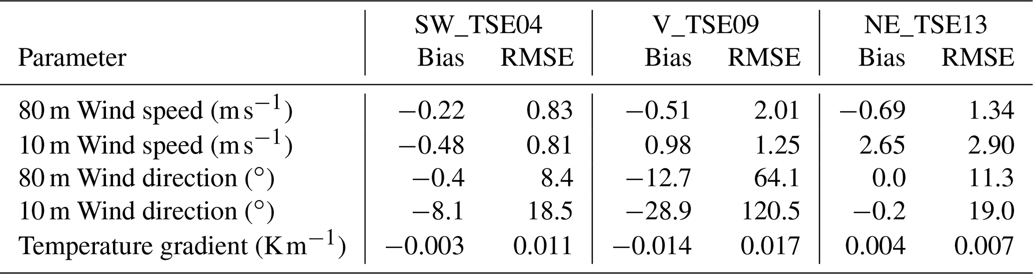
Wind speed, wind direction, and the potential temperature gradient are also compared with met tower measurements in Fig. 7. The modeled wind speed and wind direction generally follow the observations at both hub height (80 m) and near the surface (10 m), with greater variability in the valley compared to on top of the two ridges. Errors quantified in terms of bias and RMSE are shown in Table 2. At hub height and along the two ridges, wind speed errors are below 1.5 m s⁻¹ and wind direction errors are below 12^∘. Within the valley, hub-height wind speed and wind direction errors are on the order of 2 m s⁻¹ and 60^∘, respectively. Both the wind speed and wind direction fluctuate much more in the valley compared to the ridges, which the model captures reasonably well considering the low wind speeds present. The temperature gradient within the valley in the model is indicative of a well-mixed region, whereas the measurements indicate more stable stratification, resulting in an RMSE of 0.017 K m⁻¹, although this stratification does vary significantly over the period of interest. This discrepancy is also evident in Fig. 6a–d where the model predicts that the 10 and 80 m locations for V_TSE09 are located below the mountain wave and in a region of more well-mixed and coherent turbulence.

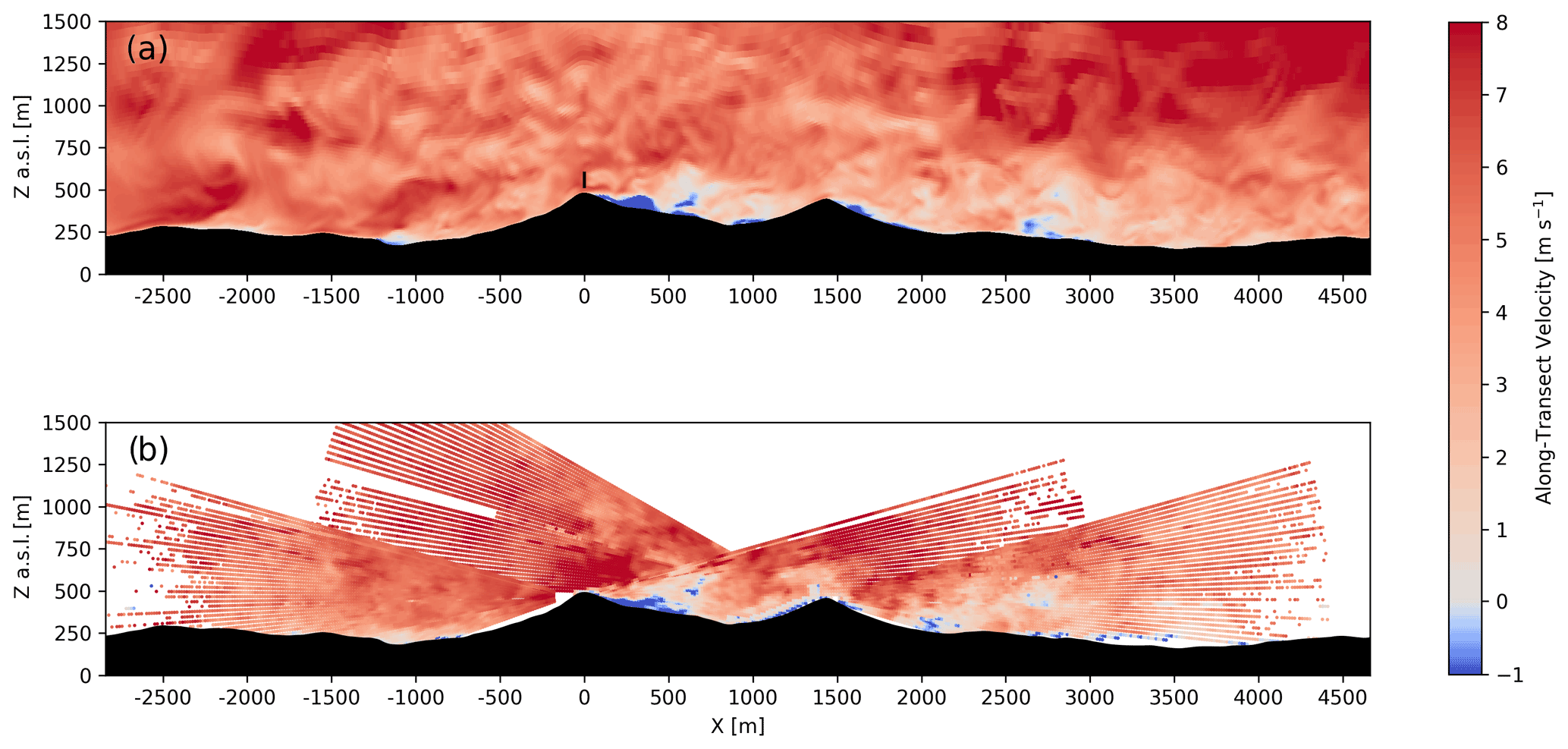
Figure 8 Instantaneous along-transect horizontal velocity during the convective case study for the model (a) and DTU multi-Doppler lidar scan (b) at approximately 13:20 UTC. The output from the model is instantaneous while the multi-Doppler measurements are over the course of a single scan, which takes about 24 s. The model transect is aligned with the wake transect and the lidar transect is aligned with the offset transect in Fig. 1. An animation of model results during the entire 1 h period is included in the supplementary material (see Video 3 in the Video supplement).

4.2 Validation of the convective case study

As for the stable case, WRF–LES–GAD is validated for the convective case using comparisons to the multi-Doppler lidar scans (Fig. 8). Unstable stratification and increased turbulent mixing lead to a turbulent mountain wake in the lee of the first ridge, which forms a recirculation zone as seen in Fig. 8. Reverse flow or recirculation near the surface in the lee of the first ridge is both predicted by the model and observed by the multi-Doppler lidar scans. Additionally, turbulent eddies are visible over the entirety of the transects in Fig. 8a and b.

Figure 9 Transect of 1 h time-averaged along-transect velocity for the model (a) and DLR lidar (b) during the convective case study with panel (c) as the difference between the DLR lidar and the model. The transects are aligned with the wake transect in Fig. 1.

The wind turbine wake interaction with the recirculation zone is shown in Fig. 9 over a 1 h time average (from 13:00 to 14:00 UTC). From Fig. 9, the recirculation zone in the lee of the first ridge extends nearly 500 m into the valley for both the model and the lidar measurements as indicated by the small difference in velocities (< 1 m s⁻¹) in Fig. 9c. In both the model and measurements, the wake does not mix with the recirculation zone or mountain wake and deflects upwards; however, the model predicts faster velocities below the wind turbine wake and above the recirculation zone.

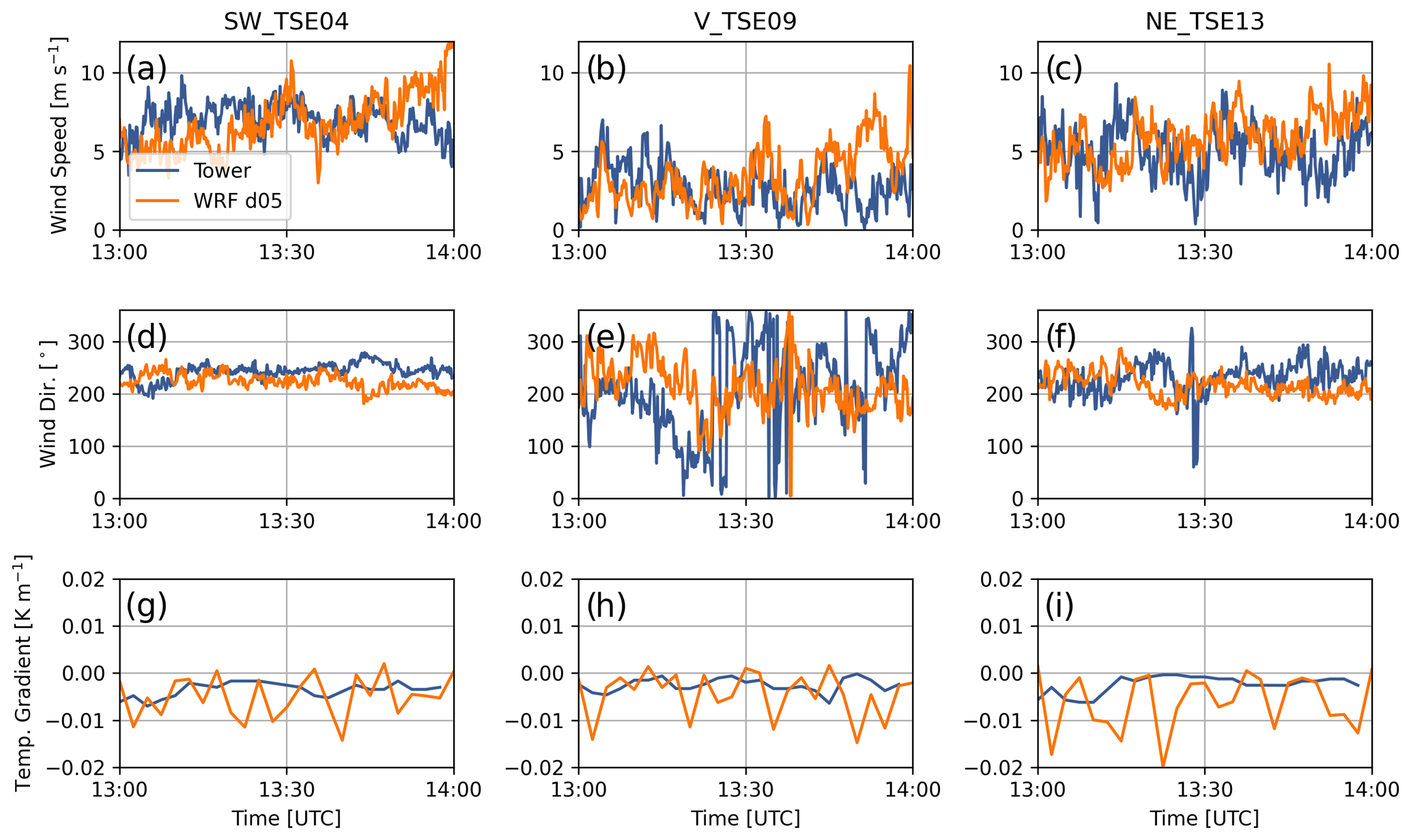
Figure 10 Comparison between meteorological tower data and WRF–LES–GAD d05 for 80 m wind speed (a–c), 80 m wind direction (d–f), and 100–10 m temperature gradient (g–i) for the convective case study. SW_TSE04 and NE_TSE13 are located on ridges, while V_TSE09 is located in the valley. Note that the model wind speed and direction are output at 10 s intervals, while the temperature is output every 150 s.

Table 3 Wind speed, wind direction, and temperature gradient bias and RMSE between WRF–LES–GAD and meteorological tower measurements for the convective case study.

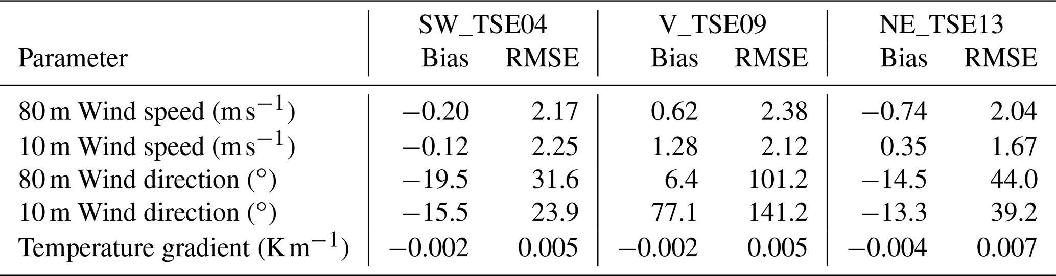
A comparison with WRF–LES–GAD and the meteorological towers in Fig. 10 during this time period shows all three parameters (wind speed, wind direction, and temperature gradient) are relatively constant with the greatest variability in the wind speed and wind direction in the valley. Errors between the model and the met tower measurements at both 80 and 10 m are shown in terms of bias and RMSE in Table 3, with wind speed errors less than 2.5 m s⁻¹. Larger errors in the near-surface wind direction within the valley are a result of lower wind speeds and increased turbulence, as compared to the flow on the ridges. Despite the variability in the modeled temperature gradient (Fig. 10g–i), the bias and RMSE values are small relative to the magnitude of the gradient itself.

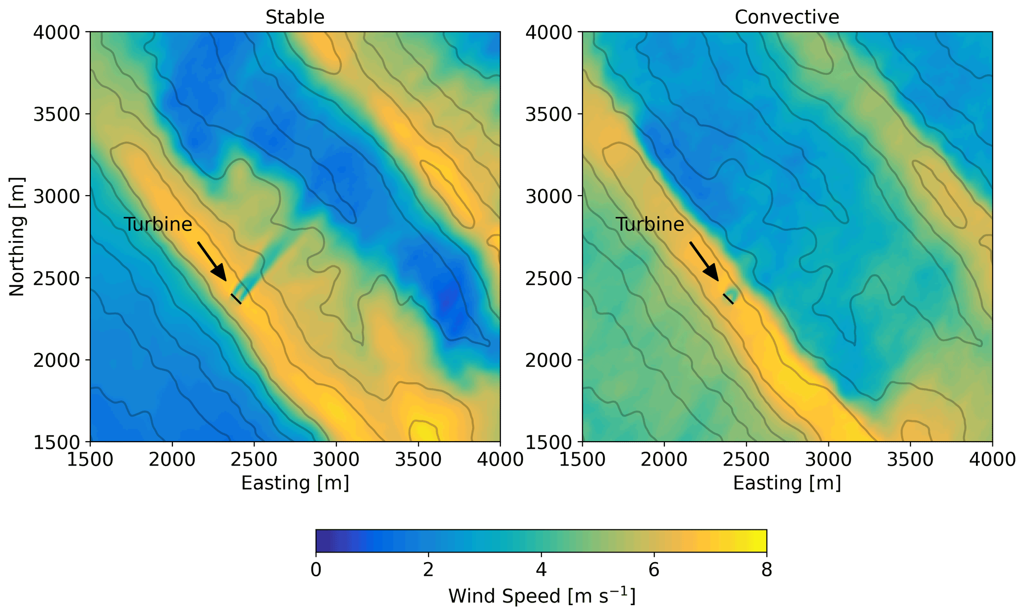
Figure 11 One-hour time-averaged wind speed contours at 80 m above the terrain for the stable case study and for the convective case study. Line contours represent 50 m changes in elevation.

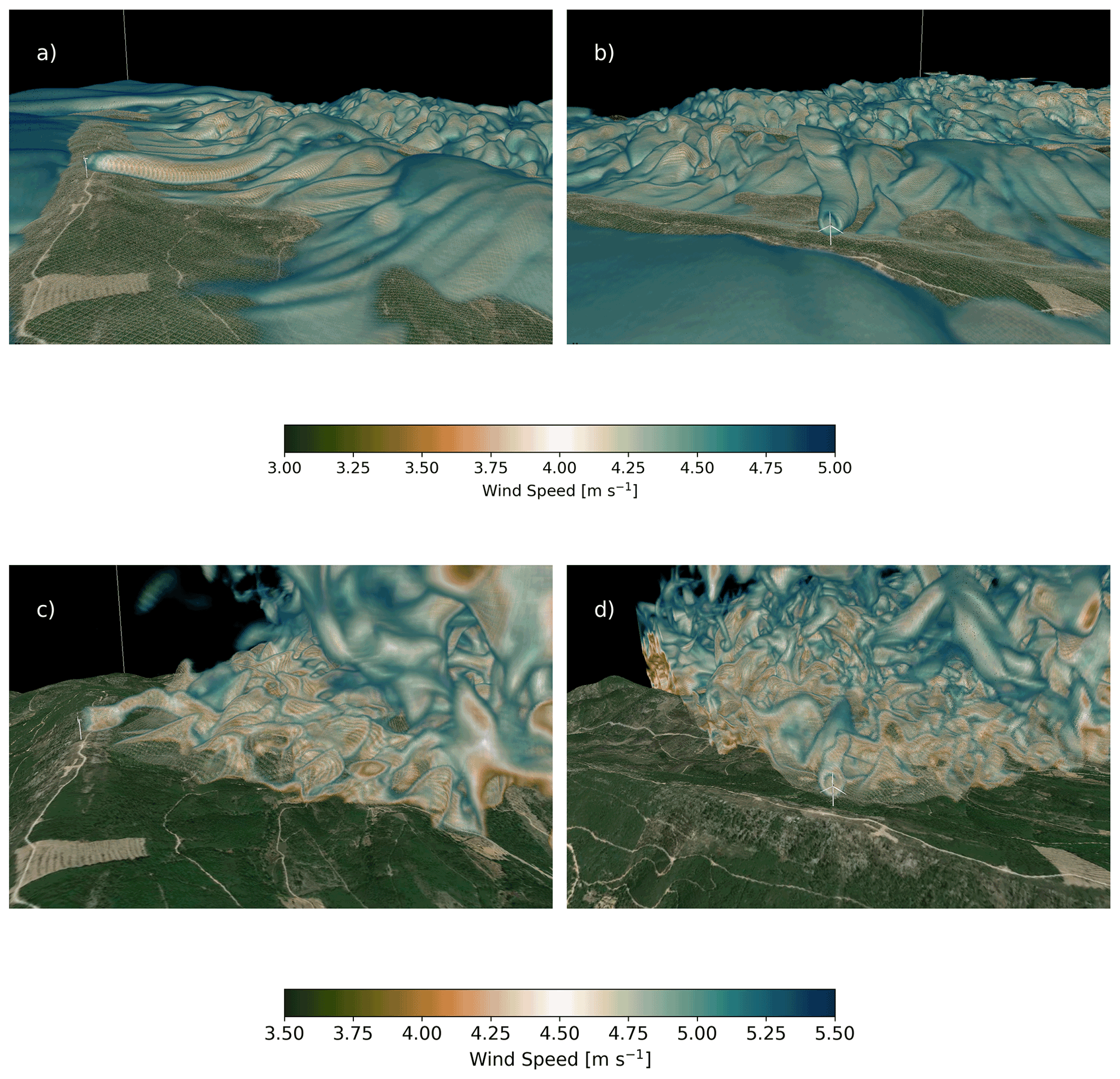
Figure 12 Three-dimensional volume rendering of wind speed for the stable case at 04:37:30 UTC (a, b) and for the convective case at 13:33:20 UTC (c, d). For the stable case, only wind speeds between 3.0 and 5.0 m s⁻¹ are shown, and the wind speeds at the first five vertical levels have been removed for clarity. For the convective case, only wind speeds between 3.5 and 5.5 m s⁻¹ are shown, and data to the south and west of the turbine have been removed for clarity. The viewpoint in panels (a) and (c) is from the southeast looking down the valley to the northwest. The viewpoint in panels (b) and (d) is southwest of the wind turbine looking to the northeast. Visualization made using VAPOR (Clyne et al., 2007).

4.3 Wind turbine wake behavior

For the complex Perdigão terrain, Menke et al. (2018) and Wildmann et al. (2019) showed that wind turbine wakes in stable stratification can be observed up to 10 rotor diameters (D) downstream, following the terrain into the valley. Our model agrees with these observations. Figure 11 shows 1 h time-averaged wind speed at approximately 80 m above the terrain for the stable case (14 June 2017, 04:30–05:30 UTC) and the convective case (13 May 2017, 13:00–14:00 UTC). The wake signature in terms of a wind speed deficit persists over 700 m into the valley for the stable case. The wake for the convective case dissipates much more quickly.

Three-dimensional visualizations provide insight into the wind turbine wake advection, meandering, and direction downstream as the flow evolves and develops over the first ridge and through the valley. Figure 12a and b show a volume rendering of wind speed at 04:37:30 UTC for the stable case. Note that the color bar has been designed to highlight the velocity deficit imparted by the wind turbine rotor. In Fig. 12a, the coherent, tubular structure that is the wind turbine wake propagates downward into the valley following the terrain. At wind speeds highlighted by the volume rendering, the wind turbine wake is the dominant structure compared to any background turbulence in the flow field. In Fig. 12a, the wake persists well into the valley and only begins to dissipate as it reaches the second ridge. Figure 12b shows how the wake meanders as it propagates into the valley. Wind veer causes the wake to deflect to the north near the second ridge.

Turbulent structures dominate the flow field in the convective case. A volume rendering of wind speed at 13:33:20 UTC for the convective case is shown in Fig. 12c and d. A similar design of the color bar that was done for Fig. 12a and b is done here for Fig. 12c and d except that the visible range of wind speeds is shifted from 3.0–5.0 to 3.5–5.5 m s⁻¹. Additionally, data to the south and west of the wind turbine have been omitted for clarity. The wake structure is not nearly as coherent and dissipates much more quickly in the convective case compared to the stable case. Figure 12c clearly shows the wake as the dominant feature on top of the first ridge. Directly behind the rotor, the wake is level but is then deflected upwards. Background turbulence begins to dominate in the lee of the first ridge and into the valley. The viewing angle used in Fig. 12d makes it so the wake is difficult to distinguish from any background turbulence except very close to the rotor.

Figure 13 One-hour time-averaged wind speed at different downstream distances for the stable and convective case studies taken along the wake transect in Fig. 1. The black circle represents the circumference of the wind turbine rotor at a constant height above sea level ($\mathrm{a}.\mathrm{s}.\mathrm{l}.$).

The recirculation zone for the convective case and the mountain wave for the stable case modulate the flow behavior in the valley. The evolution of these phenomena, their interaction with the wind turbine wake, and any spatial heterogeneity in the flow can be visualized using y–z cross sections of the wake at different downstream distances. Figure 13 shows 1 h time-averaged wind speed for the two stability cases at distances of 1D, 2D, 3D, and 4D along the wake transect (see Fig. 1). For the stable case, the wake propagates downward, following the terrain, above the slower near-surface winds. Additionally, the upper half of the wake veers in the positive y direction leading to an ellipsoid shape for the wake. This stretching of the wake due to the veer in the inflow is characteristic of stable conditions (Lundquist et al., 2015; Abkar et al., 2016; Bromm et al., 2017; Churchfield and Sirnivas, 2018; Englberger and Dörnbrack, 2018; Bodini et al., 2017), while the amount of veer in the wake depends on the shape and magnitude of the inflow veer (Englberger and Lundquist, 2020). For the convective case, we see that as the flow follows the terrain down into the valley, the recirculation zone and mountain wake rise in height. The wake structure is circular and much more coherent at distances of 1D and 2D compared to further downstream; however, a wind speed deficit is still clearly visible above the recirculation zone further downstream. The wake also drifts slightly in the positive y direction, but this is due to the slight misalignment between the wake transect and the mean wind direction.

To further quantify wake behavior in the Perdigão terrain, we determine the wake center locations downstream of the wind turbine. Using the model data, we extract 1 h time-averaged velocity profiles at distances of 1D, 2D, 3D, and 4D from the rotor along the wake transect. We also extract 1 h time-averaged velocity profiles along the offset transect. Since the terrain is similar on the nearly parallel transects, the velocity deficit can be calculated by taking the difference between the profiles along the offset transect and the profiles along the wake transect. We follow a similar procedure with the observations. The DLR lidar represents the velocity profiles along the wake transect, while the DTU lidar represents the velocity profiles along the offset transect. In these velocity deficit profiles, the vertical wake centers can then be determined by finding the vertical location at which the velocity deficit is greatest.

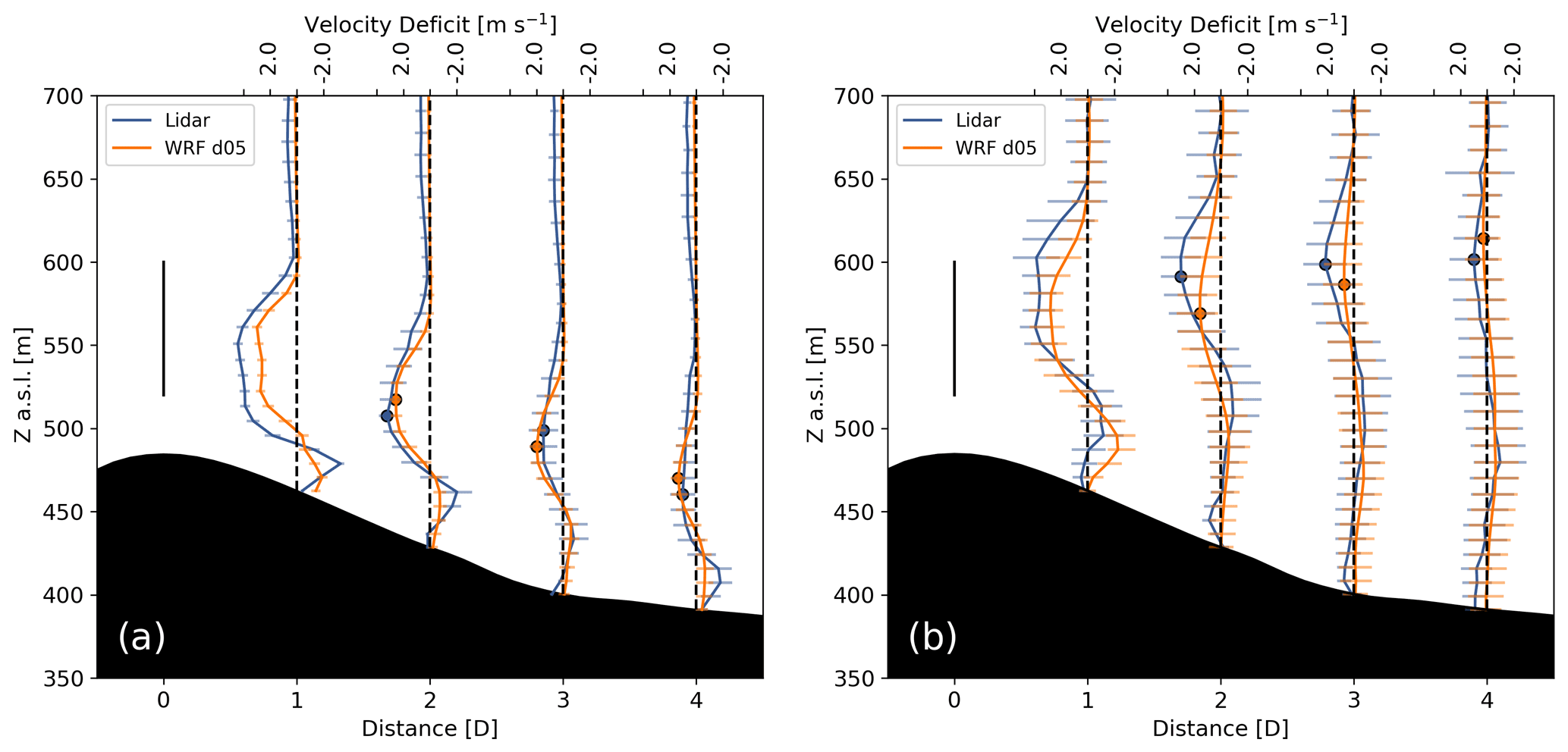
Figure 14 One-hour time-averaged profiles of velocity deficit along the wake transect based on the lidar measurements and calculated in WRF–LES–GAD d05 for the (a) stable and (b) convective case studies. The error bars correspond to ± σ, where σ is the standard deviation during the averaging period. The solid black line represents the diameter of the wind turbine rotor.

In Fig. 14, the vertical wake centers follow similar patterns between the measurements and model with the wake centers tracking downwards in the stable case and upwards in the convective case. For the stable case, the wake deflects downwards nearly 100 m in the model and 90 m in the measurements at 4D downstream. At the same downstream distance, for the convective case, the wake deflects upwards above the hub height as high as 54 m in the model and 42 m in the measurements. Additionally, an acceleration occurs in the velocity profiles for both case studies below the wake. This speedup is more apparent for the stable case but is still clear for the convective case in the near wake. While the speedup could be due to the small differences in terrain between the two transects, it is more likely due to flow being channeled beneath the wake and above the slower near-surface wind speeds; this is consistent with the observation that this near-surface speedup occurs in LES of wakes in flat terrain (Vanderwende et al., 2016).

5 Conclusions

The multi-scale WRF–LES–GAD modeling framework has been used here to simulate wind turbine wake propagation in complex terrain under different atmospheric stability conditions, with horizontal grid resolutions ranging from 6750 m on the mesoscale domain to 10 m for the finest LES domain. This setup allows the simulations to capture the interplay between terrain, atmospheric stability, and wind turbine wake dynamics. To the authors' knowledge, this study is the first to combine the effects of highly complex terrain with a wind turbine GAD parameterization for real large-eddy simulations in non-neutral stability conditions. The WRF–LES–GAD framework was applied to a stable case study with a mountain wave and a convective case study with a recirculation zone, and the simulations were compared to field observations from both in situ and remote sensing instrumentation.

In the stable case, the wind turbine wake is deflected downward, following the terrain along with the mountain wave. The general characteristics of the mountain wave were well captured by the model over the extent of the roughly 8 km domain in comparisons with meteorological towers, a tethered lifting system, and lidar data. The wind speeds within the wave were slightly underestimated, which resulted in underprediction of the wavelength for the mountain wave. Notably, the mountain wave caused the wake to deflect downwards into the valley. At four rotor diameters downstream of the wind turbine, the wake deflected downwards on average nearly 100 m below the hub height, consistent with observations. Further, the stable wake structure stretched from a circular wake into an ellipse due to veer in the wind profile.

In the convective case, the wake was lofted above the terrain and above the original elevation of the wake as a result of the recirculation zone that formed in the lee of the first ridge. With unstable thermal stratification, a mountain wake formed in the lee of the first ridge. Averaged over the hour, we observed a 500 m long recirculation zone in the valley, consistent with observations. The formation of a recirculation zone resulted in the wind turbine wake deflecting upwards. The wake deflected an average of 54 m above hub height at four rotor diameters downstream, compared to 42 m in the lidar data. In the convective case, the wake maintains a circular structure downwind but diffuses more rapidly than in the stable case due to increased ambient turbulence.

The WRF–LES–GAD framework presented here exhibits good agreement with field observations during the Perdigão field campaign, demonstrating its suitability for examining turbine–airflow interactions and wake evolution in realistic settings involving complex terrain and varying atmospheric stability. The ability of the model to capture different wind turbine wake behavior over complex terrain under stable and convective conditions indicates the model's ability to integrate both mesoscale, i.e., regional winds and stability, and local microscale flow phenomena which influence the wake behavior. We expect that the conclusions in terms of the wind turbine wake behavior would hold for most convective and stable atmospheric conditions at the Perdigão site as long as the phenomena of interest (recirculation zones and mountain waves) are present.

Other flow phenomena could be modeled using the multi-scale WRF–LES–GAD framework to examine wind turbine wake behavior under other conditions. Further studies at the Perdigão site may also include comparisons with observed turbulence quantities. Of particular interest is the effect of turbulence closure models (Kirkil et al., 2012; Zhou and Chow, 2012) on the detailed behavior of the background turbulence and its interactions with the wind turbine wake. As more wind turbines are sited in complex terrain, WRF–LES–GAD will be a useful tool for modeling the effects of surface roughness, terrain steepness, and atmospheric forcing on wake dynamics in these environments.

Appendix A: Sensitivity of model results to grid resolution

Nested WRF–LES–GAD simulations provide increasingly detailed flow predictions according to the resolution of both the terrain and land-use data, as well as the ability to resolve turbulent flow structures. Further, nesting from 6750 to 10 m resolution allows the finest 10 m grid to represent the turbine using the generalized actuator disk model and still be influenced by mesoscale forcing from the larger domains. This appendix quantifies some of the differences between results on different grid nesting levels.

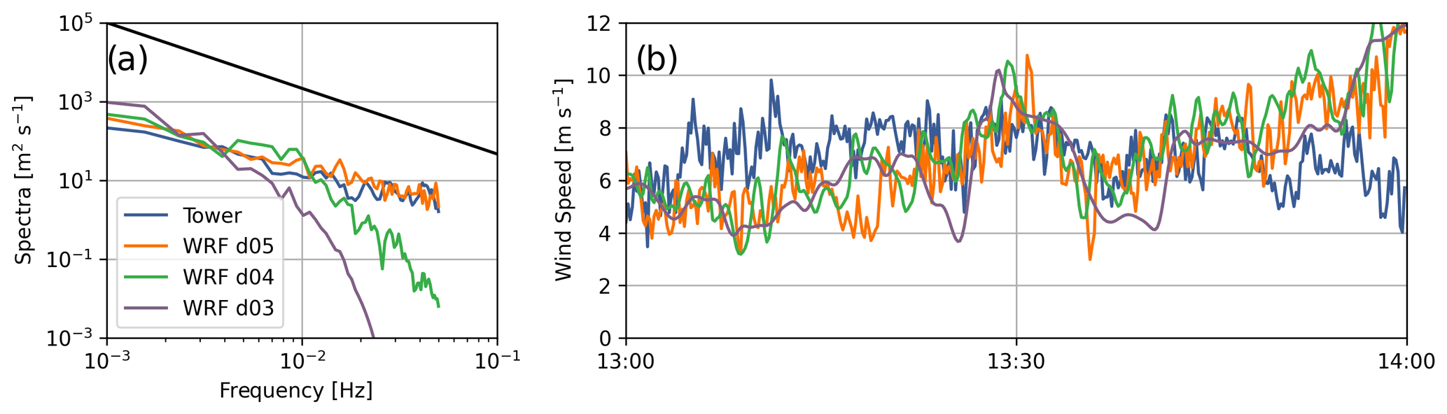
Figure A1 Comparison of (a) time series and (b) spectra between SW_TSE04 tower data and WRF–LES–GAD d05 (Δx = 10 m), d04 (Δx = 50 m), and d03 (Δx = 150 m) for 80 m wind speed at SW_TSE04 for the convective case study. The $-\mathrm{5}/\mathrm{3}$ inertial subrange power law is provided in black for reference. Note that the model wind speed is output at 10 s intervals; therefore, the highest resolvable frequency with this time series is 0.05 Hz.

The power spectral density of the 80 m wind speed signals shown in Fig. A1a illustrates that higher-frequency turbulence is captured as the grid resolution increases. The spectra are computed using Welch's method (Welch, 1967). The spectra from the measurements at SW_TSE04 roughly follow an inertial subrange slope of $-\mathrm{5}/\mathrm{3}$ following Kolmogorov (1941). The spectra for d05 also have an inertial subrange slope of $-\mathrm{5}/\mathrm{3}$ and similar energy content to the measurements. Domains d04 and d03 contain a drop-off in the wind speed spectra as is typical of models with finite-difference discretization schemes. The effective resolution for WRF is ≈7Δx (Skamarock, 2004). For wind speeds in the range of 6–8 m s⁻¹, the grid cutoff frequency at the effective resolution is 0.1, 0.02, and 0.007 Hz for d05, d04, and d03, respectively. Therefore, only d05 can resolve small-scale features like those observed at SW_TSE04 and that affect wind turbine wake dissipation.

Figure A1b shows the 80 m wind speed for d05 (Δx = 10 m), d04 (Δx = 50 m), and d03 (Δx = 150 m) as well as the measurements at SW_TSE04 with error metrics in Table A1. The bias and RMSE values for all three domains are similar, indicating that there is no significant reduction in errors at this particular location when nesting to finer grid resolution. The errors are driven more by the background flow, which will not change very much between the domains.

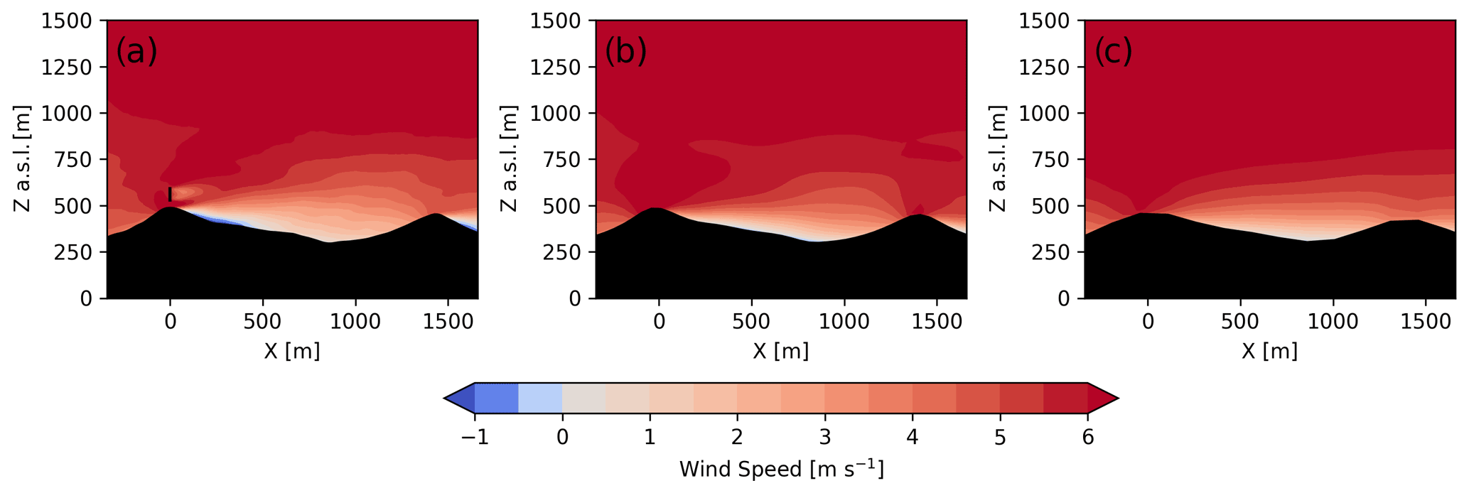
Figure A2 Transect of 1 h time-averaged wind speed for (a) d05 (Δx = 10 m), (b) d04 (Δx = 50 m), and (c) d03 (Δx = 150 m) during the convective case study.

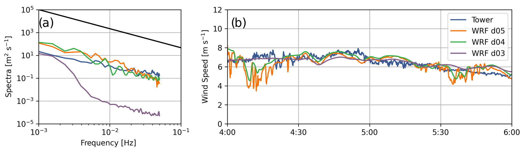
Figure A3 Comparison of (a) time series and (b) spectra between SW_TSE04 tower data and WRF–LES–GAD d05 (Δx = 10 m), d04 (Δx = 50 m), and d03 (Δx = 150 m) for 80 m wind speed at SW_TSE04 for the stable case study. The $-\mathrm{5}/\mathrm{3}$ inertial subrange power law is provided in black for reference. Note that the model wind speed is output at 10 s intervals; therefore, the highest resolvable frequency with this time series is 0.05 Hz.

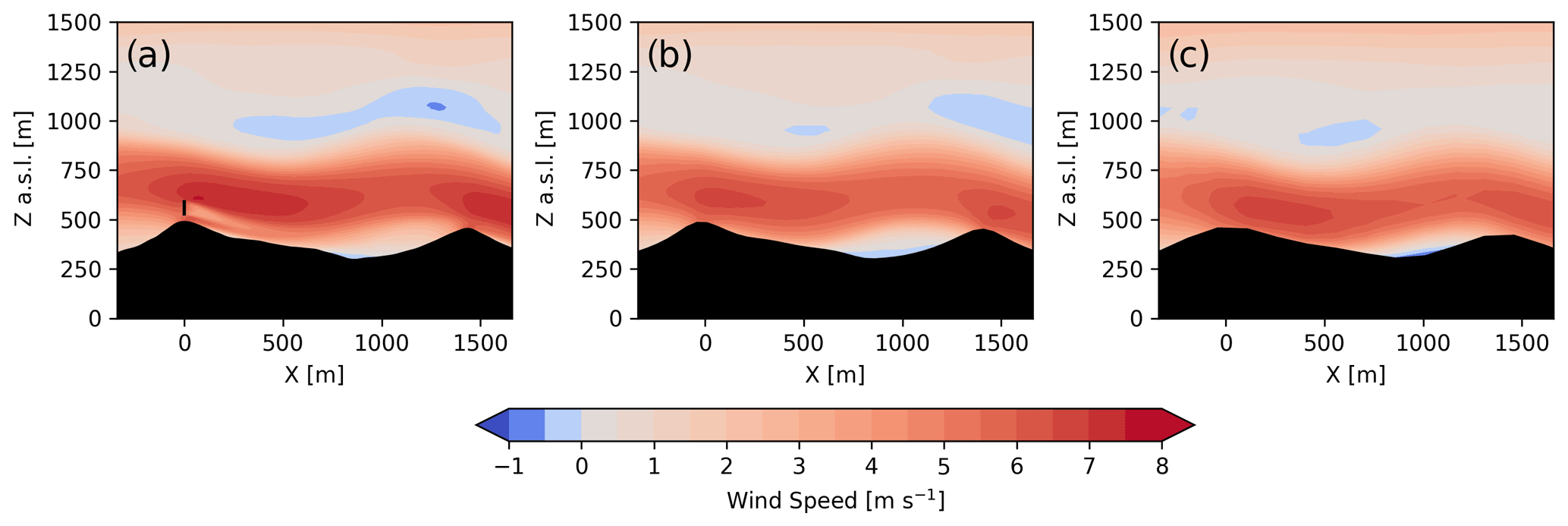
Figure A4 Transect of 1 h time-averaged wind speed for (a) d05 (Δx = 10 m), (b) d04 (Δx = 50 m), and (c) d03 (Δx = 150 m) during the stable case study.

In addition to the smaller-scale turbulence resolved on d05, steeper terrain slopes are also resolved on d05 compared to domains d04 and d03. This directly affects whether the flow recirculates in the lee of the first ridge as illustrated in Fig. A2, which shows 1 h time-averaged transects of wind speeds across the wind turbine rotor plane (note that the turbine is only parameterized on d05). While the recirculation zone is resolved on d05 (Fig. A2a), the gentler resolved slopes d04 and d03 do not induce recirculation on those domains (Fig. A2b and c). Recall that lidar observations in Fig. 9 showed recirculation in the lee of the first ridge. Put together, the effects of increased grid resolution and terrain resolution on d05 provide a more accurate representation of the observed flow features including the turbine wake.

Table A1 Eighty-meter wind speed bias and RMSE between WRF–LES–GAD on domains d03, d04, and d05 and SW_TSE04 tower measurements for the convective case study from 13:00–14:00 UTC.

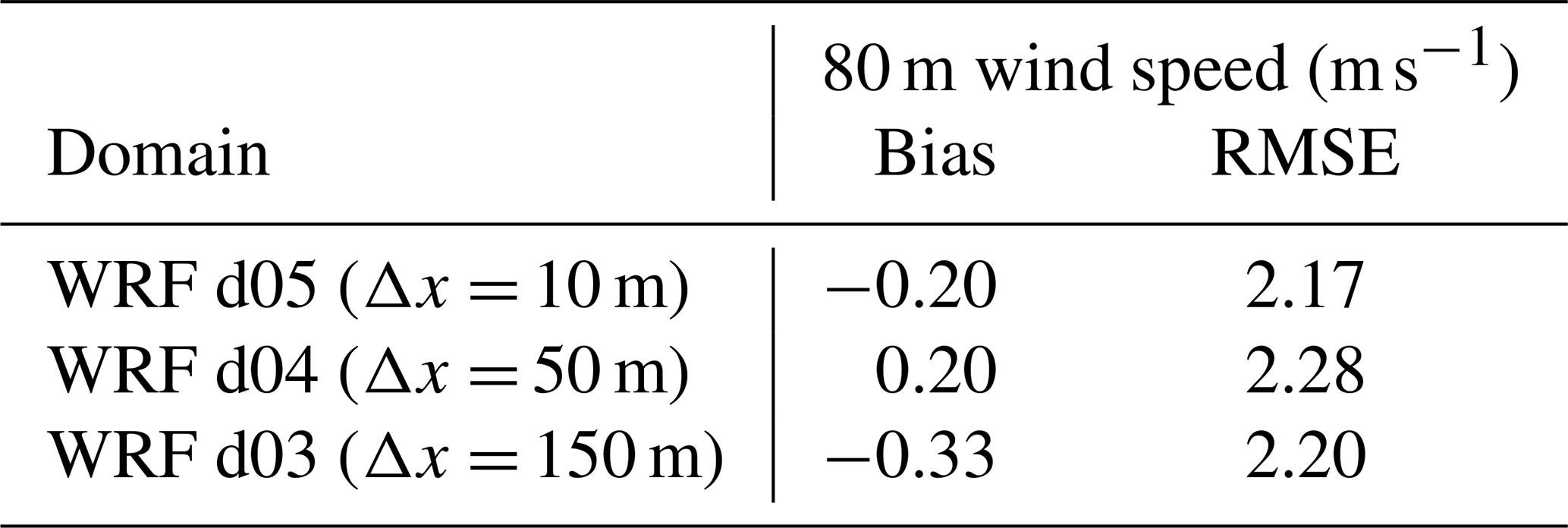
Table A2 Eighty-meter wind speed bias and RMSE between WRF–LES–GAD on domains d03, d04, and d05 and SW_TSE04 tower measurements for the stable case study from 4:00–6:00 UTC.

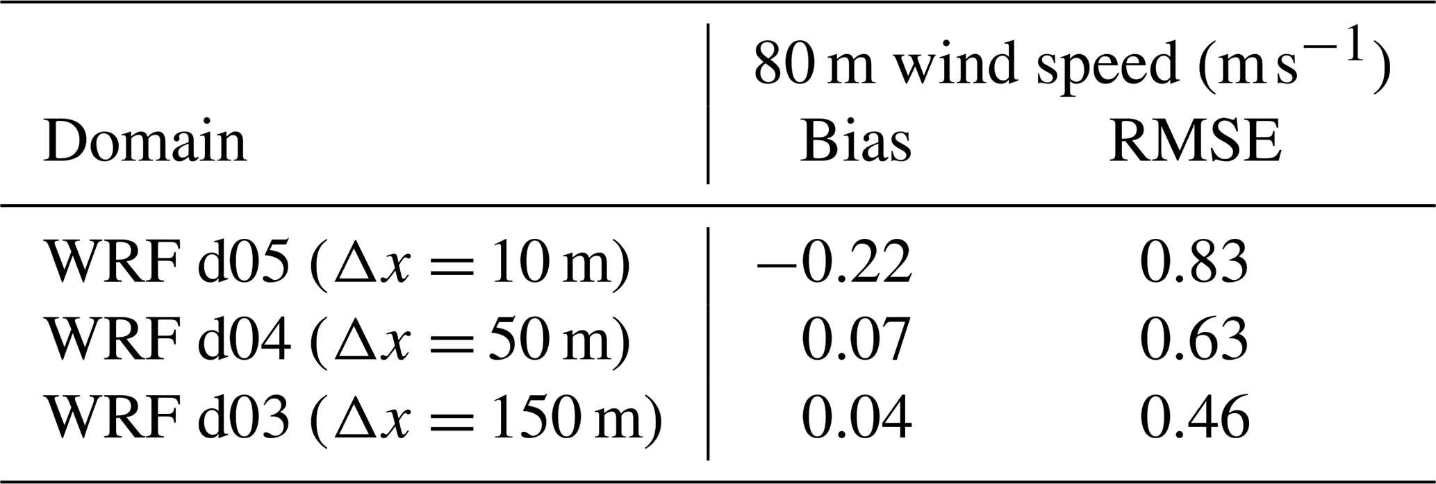
Figure A3 shows wind speed and energy spectra for the stable case study. It is clear in Fig. A3b that d03 and d04 show wind speeds much smoother than those observed by the tower. The finest domain, d05, is able to capture some fine-scale turbulent variability in the first and last parts of the 2 h time period but not in between. We see this in the spectra in Fig. A3a, where high-frequency turbulence is underestimated in the model compared to the meteorological tower. The energy is shifted to lower frequencies, thus overestimating the energy content at larger scales compared to the observations. Note that overall the energy content is lower for the stable compared to the convective case. This, in part, explains why the effect of the grid cutoff frequency is less pronounced compared to Fig. A1. Despite the expected limitations of the model to fully capture turbulence in the stable case, we note that the wind turbine wake behavior is largely determined by the mountain wave, which is governed by the internal Froude number and shows limited sensitivity to small-scale turbulence and increasing grid resolution (Fig. A4). The bias and RMSE values in Table A2 for all three domains are similar, but the values do indicate slightly higher bias and RMSE on d05 due to the greater turbulent variability (whereas d03 and d04 are closer to the observed mean velocities but cannot capture the turbulence at all). In conclusion, for the stable case study, large-scale dynamics (the mountain wave) do not require a 10 m grid, but wake and turbulence dynamics do.