the Creative Commons Attribution 4.0 License.
the Creative Commons Attribution 4.0 License.
 | 08 Mar 2022
Can reanalysis products outperform mesoscale numerical weather prediction models in modeling the wind resource in simple terrain?
Vincent Pronk
Mike Optis
Julie K. Lundquist
Patrick Moriarty
Caroline Draxl
Avi Purkayastha
Ethan Young
Mesoscale numerical weather prediction (NWP) models are generally considered more accurate than reanalysis products in characterizing the wind resource at heights of interest for wind energy, given their finer spatial resolution and more comprehensive physics. However, advancements in the latest ERA-5 reanalysis product motivate an assessment on whether ERA-5 can model wind speeds as well as a state-of-the-art NWP model – the Weather Research and Forecasting (WRF) Model. We consider this research question for both simple terrain and offshore applications. Specifically, we compare wind profiles from ERA-5 and the preliminary WRF runs of the Wind Integration National Dataset (WIND) Toolkit Long-term Ensemble Dataset (WTK-LED) to those observed by lidars at a site in Oklahoma, United States, and in a United States Atlantic offshore wind energy area. We find that ERA-5 shows a significant negative bias () at both locations, with a larger bias at the land-based site. WTK-LED-predicted wind speed profiles show a limited negative bias () offshore and a slight positive bias () at the land-based site. On the other hand, we find that ERA-5 outperforms WTK-LED in terms of the centered root-mean-square error (cRMSE) and correlation coefficient, for both the land-based and offshore cases, in all atmospheric stability conditions. We find that WTK-LED's higher cRMSE is caused by its tendency to overpredict the amplitude of the wind speed diurnal cycle. At the land-based site, this is partially caused by wind plant wake effects not being accurately captured by WTK-LED.
- Article
(3772 KB) - Full-text XML
-
Supplement
(935 KB) - BibTeX
- EndNote


This work was authored in part by the National Renewable Energy Laboratory, operated by Alliance for Sustainable Energy, LLC, for the U.S. Department of Energy (DOE) under contract no. DE-AC36-08GO28308. The views expressed in the article do not necessarily represent the views of the DOE or the U.S. Government. The U.S. Government retains and the publisher, by accepting the article for publication, acknowledges that the U.S. Government retains a nonexclusive, paid-up, irrevocable, worldwide license to publish or reproduce the published form of this work, or allow others to do so, for U.S. Government purposes.
Wind energy development requires an accurate characterization of the wind resource at the heights swept out by commercial wind turbine rotor blades (Brower, 2012). Directly measuring the wind speed aloft for the extensive periods of time required for an accurate wind resource assessment can be challenging from both a technical and financial point of view. For land-based sites, there are several major factors that can pose limitations to the installation of tall meteorological towers or remote sensing devices, including complex topography, road access, availability of electrical power, and excessive cost. When considering offshore regions, where an unprecedented growth in installed wind capacity is currently taking place worldwide (Musial et al., 2016; Bureau of Ocean Energy Management, 2018), the challenges connected to having direct observations of hub-height wind speed are even more severe. Floating lidars represent a state-of-the-art source of offshore wind speed observations aloft (Carbon Trust Offshore Wind Accelerator, 2018; OceanTech Services/DNV GL, 2022); however, their prohibitive cost still severely limits their availability worldwide. As a result of this constrained scenario, numerical weather prediction (NWP) models at the mesoscale and reanalysis products are frequently used (Draxl et al., 2015; Hahmann et al., 2020; Dörenkämper et al., 2020; Optis et al., 2020) to characterize the wind resource at the heights of interest for wind energy development, for both land-based and offshore locations.
Reanalysis products are convenient to use given their global coverage and publicly available data. In general, reanalysis products incorporate global measurements of atmospheric variables to produce a 3D-gridded, hindcast, best estimate of the state of the atmosphere. Reanalysis products typically provide multiple decades of data and are regularly updated (Schwartz et al., 1999; Compo et al., 2011; Gelaro et al., 2017; Bloomfield et al., 2018). While very convenient for wind resource studies, the coarse spatial (∼1∘) and temporal resolution (usually 6 h) can produce inaccurate estimates of the wind resource. Specifically, previous validation studies at land-based sites have led to a wide variety of uncertainties associated with the product used, the location, the vertical level, and the vertical and horizontal spatial approximation technique used (Kubik et al., 2013; Rose and Apt, 2015; Ramon et al., 2019; Molina et al., 2021). Offshore, reanalysis products generally have better skills, and they have been used to create atlases of either wind resource or wind energy potential. Zheng et al. (2018) quantified the global offshore wind resource using the ERA-Interim reanalysis product (Dee et al., 2011), while Soares et al. (2020) recently evaluated the global offshore wind energy potential using the more recent ERA-5 product (Hersbach et al., 2020). However, validating such reanalysis predictions against hub-height observations has rarely been done because of the scarcity of offshore wind speed observations at the heights of interest for commercial wind development. Sheridan et al. (2020) recently validated three reanalysis products using data at one single height from a floating lidar in the United States Eastern Seaboard and found that ERA-5 had the best performance out of the four considered reanalysis products. Similar validations have been performed in northern Europe, especially focusing on low-level jet events (Kalverla et al., 2019; Hallgren et al., 2020).
By comparison, NWP models generally provide more accurate estimates of the wind resource but are much more expensive to run. NWP models use a large-scale atmospheric product, such as a reanalysis product, as external forcing, while using higher spatial and temporal resolution to simulate more comprehensive physics. Several studies have applied NWP models to wind resource assessment (an extensive review can be found in Al-Yahyai et al., 2010) at a variety of temporal and spatial scales. Draxl et al. (2015) developed an NWP model-based wind speed atlas for the continental United States, and similar efforts have been completed for the European continent (Hahmann et al., 2020; Dörenkämper et al., 2020). Recently, NWP models have also been used to create offshore wind resource assessment datasets (Rybchuk et al., 2021). By providing high-resolution wind speed data, NWP models are beneficial for assessing the wind resource at specific sites of interest for wind energy development. However, the development of NWP-based wind resource datasets is computationally expensive, especially when considering the fine horizontal, vertical, and temporal resolutions, as well as long-term periods of record.
Within this context, the latest reanalysis product, ERA-5 (Hersbach et al., 2020), comes with significant advancements compared to previous products, in terms of both spatial (∼32 km horizontally) and temporal (1 h) resolutions. These improvements motivate an analysis on whether ERA-5 is capable of modeling wind speeds with an accuracy comparable if not superior to the state-of-the-art mesoscale NWP model – the Weather Research and Forecasting (WRF) Model (Skamarock et al., 2019), as part of the initial runs for the WIND Toolkit Long-term Ensemble Dataset (WTK-LED). A similar analysis was performed for the WRF-based New European Wind Atlas by Dörenkämper et al. (2020), who found a significant negative bias for ERA-5. For our evaluation, we consider vertical profiles of wind speed up to 200 m and focus on two sites of primary importance for present and future wind energy development in the United States. As an example of a land-based site, we consider the U.S. Department of Energy's Atmospheric Radiation Measurement (ARM) Southern Great Plains (SGP) long-term measurement site near Lamont, Oklahoma. Several wind plants have been built near this location in the past decade, and an international field experiment (the American WAKE experimeNt, AWAKEN) is currently being planned at this site to better characterize the atmosphere–wake interactions (Moriarty et al., 2020). Offshore, we focus on two floating lidars recently developed by the New York State Energy Research and Development Authority (NYSERDA) along the United States Eastern Seaboard, where an unprecedented development of offshore wind energy in the United States is currently being planned (Bureau of Ocean Energy Management, 2021). We describe the datasets in Sect. 2, where we also introduce the performance metrics we adopt in the analysis. The results of the evaluation of both WTK-LED and ERA-5 are presented in Sect. 3, where we also focus on the variability of the assessed performance with height, wind direction, and atmospheric stability. Finally, we conclude our analysis and suggest future work in Sect. 4.
While complex terrain likely remains too challenging for an accurate wind speed representation by ERA-5 and will be the subject of future work, here we focus our analysis on simple terrain. More in detail, we perform a reanalysis and mesoscale model validation at two locations – one on land and one offshore. At both sites, publicly available hub-height wind speed observations are used.
For our land-based test case, we focus on the ARM SGP Central Facility (C1) site near Lamont, Oklahoma (Fig. 1). The SGP Central Facility site is located in a fairly flat area with an elevation ranging from just ∼270 to 390 m a.s.l. in the area surrounding the site. As a result, the land is used primarily for agricultural purposes. Several wind power plants were built in the area in the last decade, as shown in the map in Fig. 1. For our analysis, we consider data from 1 January 2018 to 31 December 2018. While both ERA-5 and lidar observations at the site cover a much longer time period, preliminary WTK-LED data for the region are available only for this 1-year period.
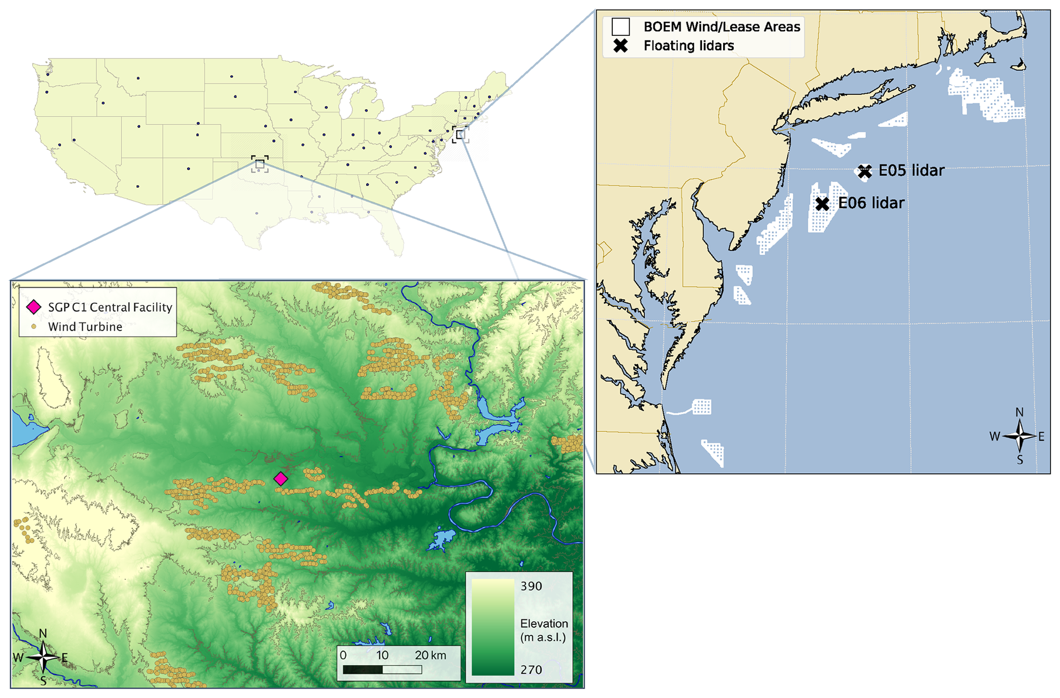
Figure 1Map of the two sites considered in our validation analysis. Digital elevation model data courtesy of the U.S. Geological Survey.
Offshore, we use wind speed observations from two floating lidars along the United States Eastern Seaboard, where several wind energy lease areas have been planned (Bureau of Ocean Energy Management, 2021) for future offshore wind energy development (Fig. 1). We consider data from 1 September 2019 to 31 August 2020 (lidar data are not available before this period, and WTK-LED was not run after it).
2.1 Observations
At the SGP Central Facility site, we consider observations from a Halo StreamLine lidar (Newsom and Krishnamurthy, 2012). We obtain horizontal wind speed data from full 360∘ conical scans by the lidar, which were performed approximately every 15 min, with 1 min needed to complete each scan. To obtain the horizontal wind speed from the line-of-sight velocity from these scans, we use the velocity–azimuth-display approach from Frehlich et al. (2006). In doing this, the horizontal wind field is assumed to be homogeneous over the scan volume (Browning and Wexler, 1968). As in Bodini and Optis (2020), we discard any measurements that have a signal-to-noise ratio lower than −21 dB or higher than +5 dB, as well as any measurements from time periods with precipitation that may significantly lower the accuracy of the measurements. The wind speed data are then averaged to obtain hourly average data. For our study, we consider data from six range gates, which correspond to heights of 65, 91, 117, 143, 169, and 195 m a.s.l. Data at lower heights are not used because of poor data quality. The analysis of the lidar data reveals how the site experiences winds mainly from the south (see 91 m wind rose in Fig. 2a), with more variability observed in winter months. Many wind plants were built around the SGP site in the last decade. At the Central Facility site, the closest wind turbines are about 3.5 km away, and Bodini et al. (2021a) showed how the site is impacted by wind plant wakes for southerly flow, especially in nighttime stable conditions. We classify atmospheric stability using near-surface (4 m a.g.l.) observations from a sonic anemometer at the C1 site. We calculate the Obukhov length as
where k=0.4 is the von Kármán constant, is the acceleration due to gravity, Tv is the virtual temperature (K), is the friction velocity (m s−1), and is the kinematic virtual temperature flux (K m s−1). All Reynolds decompositions are calculated with a 30 min averaging period (De Franceschi and Zardi, 2003; Babić et al., 2012). We consider stable conditions for m, unstable conditions for m, and near-neutral otherwise. Figure 2b–d show 24×12 heat maps of the frequency of stable, unstable, and neutral conditions, respectively. A clear diurnal pattern emerges, with stable conditions being typical of the nighttime hours and unstable conditions occurring in daytime convective periods. Also, summer shows more extended unstable cases compared to winter months. On the other hand, near-neutral conditions are relatively rare at the site, occurring most often during morning and evening transitions. Finally, we consider measurements of sensible and latent heat fluxes from a flux station at the C1 site, which includes a sonic anemometer and an infrared gas analyzer, at 4 m a.g.l. Details on the calculation of the fluxes from these instruments are described in Fischer (2004) and follow the correction proposed in Webb et al. (1980).
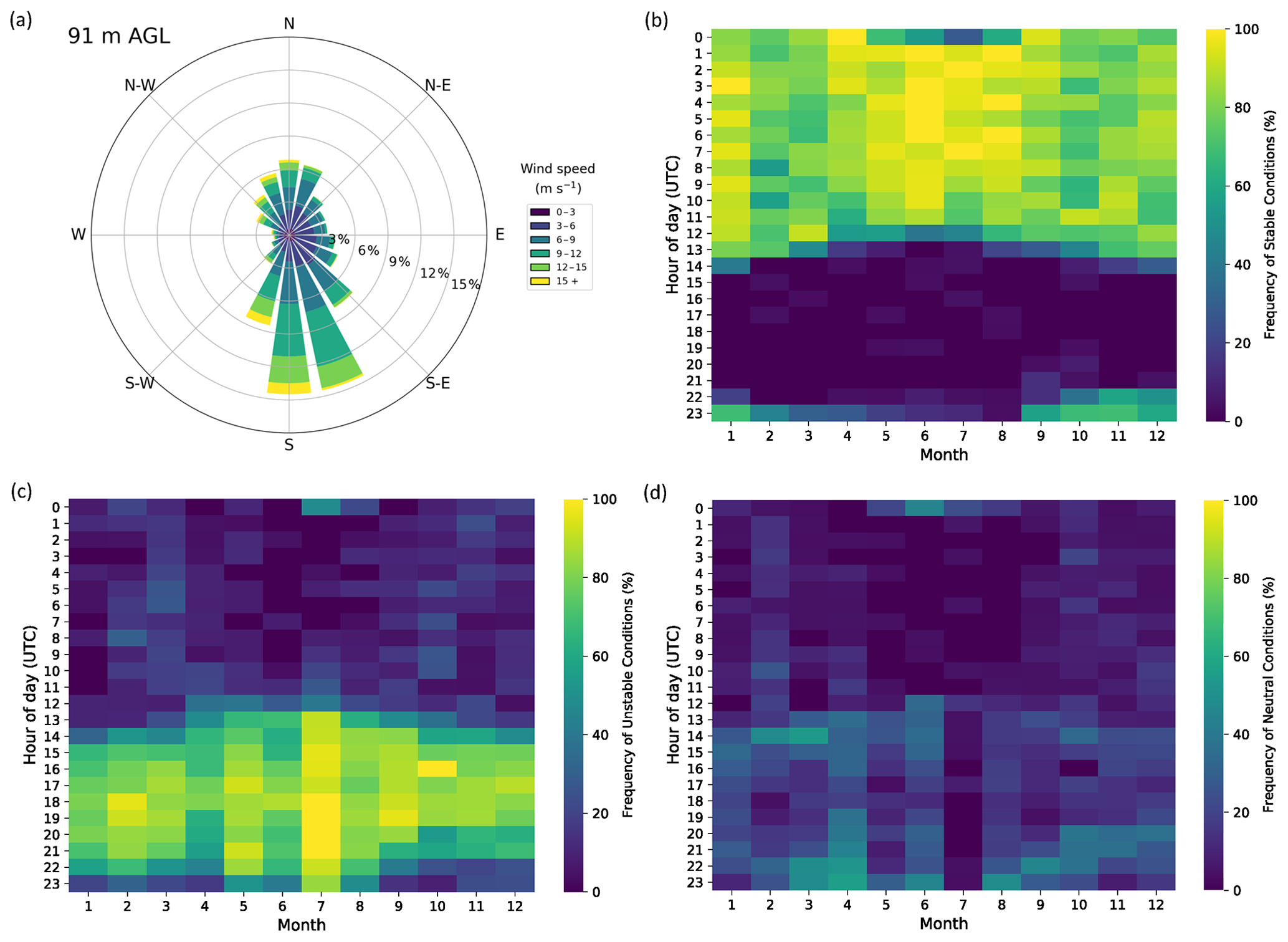
Figure 2(a) Wind rose showing the distribution of wind speeds at 91 m a.g.l. for 2018, using lidar observations at the SGP Central Facility site. (b) The 24×12 heat map of the frequency of stable conditions at the site, classified in terms of the surface Obukhov length. (c) Same but for unstable and (d) neutral conditions.
Offshore, we consider observations of wind speed from two floating lidars off the coast of New Jersey. The New York State Energy Research and Development Authority (NYSERDA) recently deployed ZephIR ZX300M lidars and made their data publicly available (OceanTech Services/DNV GL, 2022). The lidar on buoy E05 is located at 39.97∘ N, 72.72∘ W; the buoy E06 lidar is located at 39.55∘ N, 73.43∘ W. The lidar observations are provided as hourly averages, after proprietary quality checks are applied to the data. Wind speed and wind direction data for both lidars are available every 20 m from 60 to 200 m a.s.l. At these sites, wind mainly flows from the southwest and northwest, as is the case further east in this region (Bodini et al., 2019, 2020), and it is generally stronger than what is observed at SGP, as shown in the wind rose at 100 m a.s.l. from lidar E05 in Fig. 3a. Due to the lack of observations from which atmospheric stability metrics can be calculated, we use WTK-LED data to classify atmospheric stability as a function of the bulk Richardson number from 0–200 m above the surface. The bulk Richardson number is calculated as
where g is the gravitational acceleration, is the average absolute virtual potential temperature across the considered layer of thickness Δz, Δθv is the virtual potential temperature difference across the layer, and ΔU and ΔV are the changes in the horizontal wind components across that same layer. We use values of Rib>0.025 to classify stable conditions, for unstable conditions, and all other values as near-neutral conditions. Figure 3b and c show the 24×12 heat maps of the frequency of stable and unstable conditions, respectively. While a clear diurnal pattern emerges when looking at similar plots at SGP, here we find little diurnal variability but a strong seasonal cycle. Summer months show the most instances of stable conditions, while winter months show primarily unstable conditions. Finally, near-neutral conditions account for up to half of the cases in certain times and show little variability across both the diurnal and annual scales.
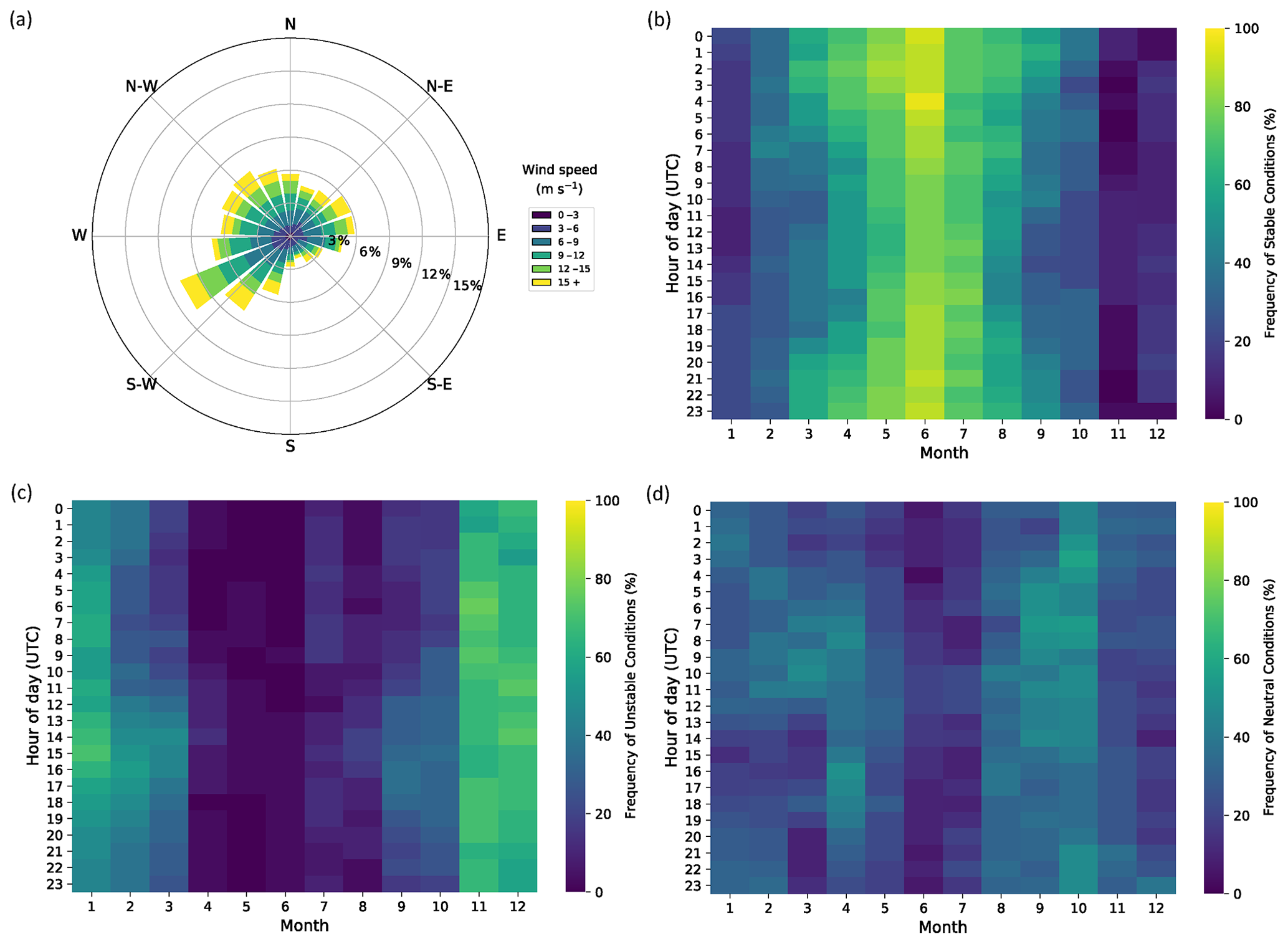
Figure 3(a) Wind rose showing the distribution of wind speeds at 100 m a.g.l. for September 2019 to August 2020, using observations from the E05 floating lidar. (b) The 24×12 heat map of the frequency of stable conditions at the E05 lidar location, classified in terms of the WTK-LED-based bulk Richardson number calculated between 0 and 200 m a.s.l. (c) Same but for unstable and (d) neutral conditions. Results from the E06 lidar are included in the Supplement.
2.2 NWP model setup
At SGP, we use WRF model data for 2018 from the preliminary National Renewable Energy Laboratory's (NREL's) Wind Integration National Dataset (WIND) Toolkit Long-term Ensemble Dataset (WTK-LED), which will update the original WIND Toolkit (WTK) (Lieberman-Cribbin et al., 2014; King et al., 2014; Draxl et al., 2015). The main WRF attributes in the WTK-LED setup are summarized in Table 1. All the main setups that have been shown to have a major impact on modeled wind speed (e.g., the choice of the planetary boundary layer scheme and of the atmospheric forcing) are the same between the offshore and land-based domains. For some other setups, different choices are made between the two domains in order to optimize and tailor the numerical simulations to the specific needs of each domain. At both sites, the simulations are initialized every month, and each simulation is initialized 2 d prior to and run up to 1 d after the end of each month. The first day of each monthly run is used as spin-up time for the model, while the second and last days are used to combine monthly runs. Model output is available at 5 min resolution, and we average the data at hourly resolution to perform the validation analysis. We consider data from the closest 2 km grid cell to the location of the lidar (the difference in terrain height between this WRF grid cell and the actual lidar location is <3 m). To match the heights at which lidar observations are available, we linearly interpolate the WRF data from the two closest levels. Given the high near-surface resolution used (see Table 1), we expect this linear interpolation to introduce only a small additional error to the analysis.
Table 1Key attributes of the WRF simulations in WTK-LED setup used in this study.
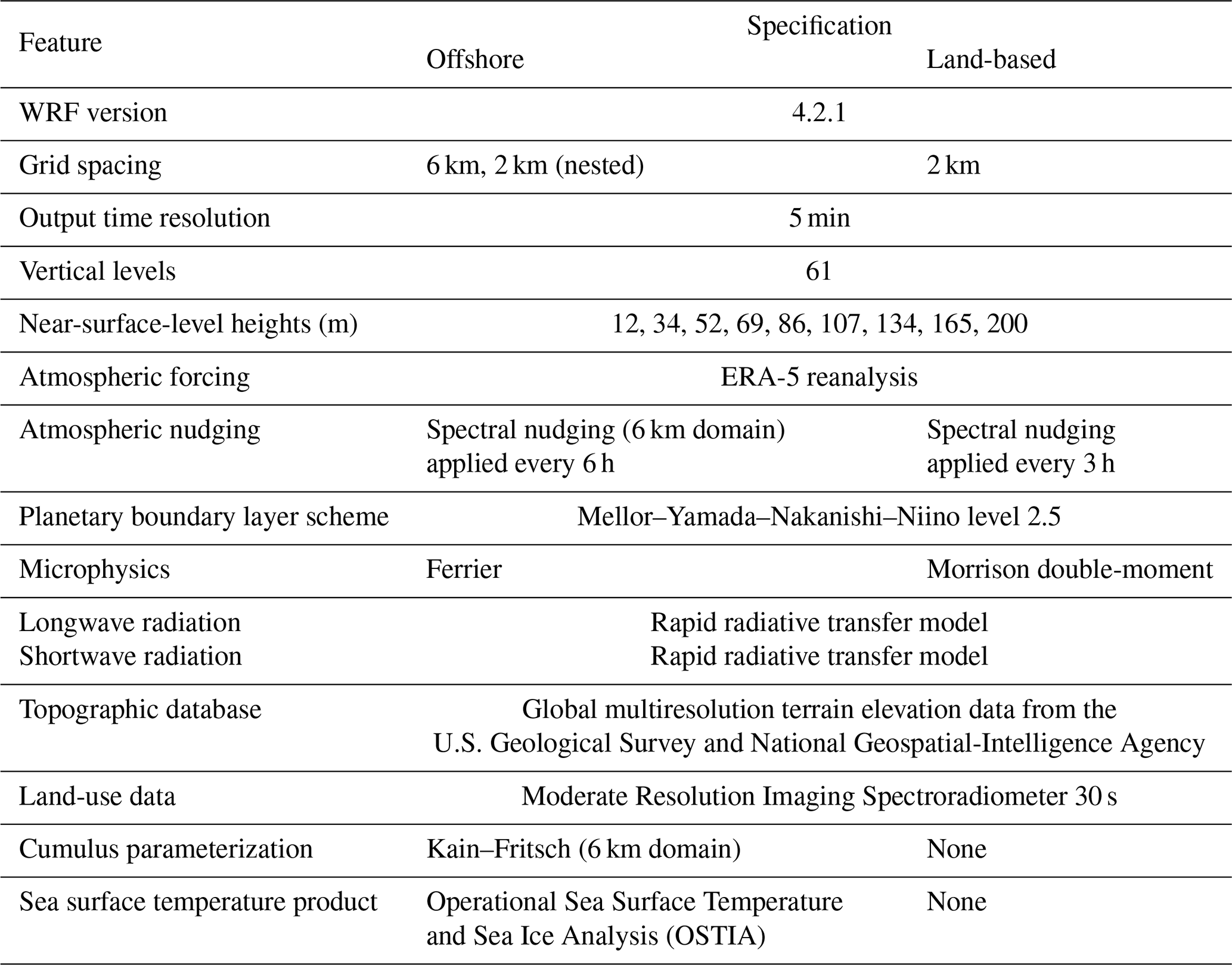
Offshore, we use WRF data from the offshore version of NREL's WTK-LED. A summary of the model setup is provided in Table 1. Similar to the land-based case, we select WTK-LED data from the closest grid cell to the location of each of the two floating lidars and linearly interpolate the WRF vertical levels to match the heights of the lidar data.
2.3 ERA-5 reanalysis
We use the state-of-the-art ERA-5 reanalysis product (Hersbach et al., 2020) to compare its skill in assessing wind resources with that of the WTK-LED product. ERA-5 provides hourly average data at 137 vertical levels and an ∼31 km horizontal resolution. In our analysis, we consider vertical levels corresponding to heights of 54, 79, 106, 137, 170, and 205 m a.s.l. As done for WTK-LED, these heights are then linearly interpolated to match those of the lidar observations. We use data from the ERA-5 grid point which is closest in space to the considered lidars. Sheridan et al. (2020) recently showed that selecting the closest grid point generally leads to better reanalysis performance compared to a linear interpolation of the four surrounding grid points, while Livingston and Lundquist (2020) used a bilinear interpolation. The coordinates of the selected ERA-5 grid point at SGP are 36.5∘ N and 97.5∘ W; offshore, we use data from the 40∘ N, 72.75∘ W grid point to compare with the E05 lidar data and at 39.5∘ N, 73.5∘ W to compare with the E06 lidar data.
2.4 Performance metrics
To quantify the skills of WTK-LED and ERA-5 in predicting the observed wind resource, we calculate, at all of the considered heights, five performance metrics.
In general, it is important to decompose a model error into bias, which quantifies the difference between modeled and observed data, and random error, which quantifies the variability of the modeled data around the mean. We decompose the root-mean-square error (RMSE) into a bias component and an “unbiased” or “centered” component of RMSE (cRMSE), following the approach in Taylor (2001). We calculate bias as
where is the mean of the modeled (by either WTK-LED or ERA-5) estimates and is the mean of the lidar observations. A perfect prediction would have a bias of 0. Next, we calculate the cRMSE as
where N is the number of data points in the considered time series, and pn and on indicate the time series values of modeled and observed wind speed, respectively. A perfect prediction would have a cRMSE of 0.
As a third performance metric, we calculate the square of the Pearson's correlation coefficient between observed and modeled wind. The correlation coefficient r measures how strong the correspondence between two variables is, and it is calculated as
where σp and σo are the standard deviations of the modeled and observed data, respectively. A perfect prediction would have a correlation coefficient of 1.
Next, we use the Earth mover's distance (EMD), also known as the Wasserstein distance (Vaseršte\ĭn, 1969; Hahmann et al., 2020), which measures the difference between two distributions. EMD is calculated as the area between two cumulative distribution functions (here, modeled and observed wind speed). This metric is an improvement on the bias metric and will catch cases where bias may be zero, despite having different modeled and observed wind speed distributions. The distribution of a perfect prediction would have an EMD of 0.
Last, we compare the standard deviation of the observed wind speed with what is predicted by WTK and ERA-5.
3.1 Mean performance
In Fig. 4, we compare the mean wind profiles from all three data sources at SGP and the NYSERDA E05 lidar. (Results from the E06 lidar are included in the Supplement because no major differences between the results from the two lidars were found.) In each panel, the solid lines indicate the mean wind profile, and the shaded bands around them represent ± the standard deviation of the data. On average, the wind resource is stronger offshore. At both sites, the ERA-5 mean wind profile underestimates the observed wind resource. Conversely, WTK-LED shows a limited overestimation of the mean wind profile at the land-based site and a slight underestimation offshore. However, in all cases, a large variability emerges so that a more detailed investigation, beyond an annual average, is required.

Figure 4Mean vertical wind speed profiles for all three data sources at (a) the land-based SGP site and (b) the offshore E05 floating lidar. The shaded bands represent ± the standard deviation of the data.
We then consider the five mean performance metrics introduced in Sect. 2.4 for both WTK-LED and ERA-5 calculated at the two sites (Fig. 5). The WTK-LED-predicted wind speed profiles show a limited positive bias () at the land-based location and a slight negative bias () offshore. However, ERA-5 shows a significant negative bias at both locations, especially at SGP, where the bias is . In general, we find little variability with height, with just a minor degradation of the bias with height for both WTK-LED and ERA-5. When considering the cRMSE, however, we find an opposite situation, with ERA-5 outperforming WTK-LED at both locations at all heights. We find satisfactory correlation at both sites, once again with ERA-5 providing marginally better values. The offshore location shows larger values (r2>0.85 for both ERA-5 and WTK-LED at all heights), likely because of the positive effects of the simpler topography on the skills of both data sources. Interestingly, we find a minor increase in r2 with height, especially at SGP. When looking at the EMD, WTK-LED significantly outperforms ERA-5 at both sites, once again with the offshore site showing better results for both data sources compared to the land-based location. Finally, when comparing the modeled and observed wind speed standard deviations, we find no clear winner between WTK-LED and ERA-5 at SGP, whereas offshore WTK-LED provides more accurate results. Given the difference in relative performance between WTK-LED and ERA-5 when considering different metrics, we will investigate the impact of wind direction, atmospheric stability, diurnal, and seasonal cycles in the next sections to investigate the potential reasons for such variability.
Figure 5Vertical profiles of mean bias, cRMSE, r2, EMD, and wind speed standard deviation at the SGP C1 site (left) and the E05 lidar (right). Results from the E06 lidar are included in the Supplement.
3.2 Impact of atmospheric stability
To assess whether the relative performance between ERA-5 and WTK-LED holds in all atmospheric stability conditions, we segregate the data at both sites. As detailed in Sects. 2.1.1 and 2.2.1, we classify atmospheric stability at SGP based on the near-surface observed Obukhov length, while offshore we base our classification on the WTK-LED-modeled bulk Richardson number, in absence of direct observations from which atmospheric stability parameters can be derived. We then calculate the vertical profiles of the five performance metrics for each stability class at the two sites (Fig. 6). The relative performance between ERA-5 and WTK-LED observed from the mean profiles with no data segregation still holds in all stability conditions: WTK-LED outperforms ERA-5 for bias EMD and, at the offshore site, standard deviation, while ERA-5 shows a better performance when considering cRMSE and r2. When analyzing how the performance of each data source varies with atmospheric stability, interesting considerations emerge.
Figure 6Vertical profiles of performance metrics segregated by atmospheric stability at the SGP C1 site (left) and at the location of the E05 lidar (right). Results from the E06 lidar are included in the Supplement.
At SGP, WTK-LED shows the best agreement with observations in unstable conditions, with a near-zero bias and EMD at all considered heights, and its lowest values of cRMSE. However, stable cases seem the most challenging to model for WTK-LED, as also noticed by Smith et al. (2018, 2019) with respect to the challenges for WRF to accurately model the frequent nocturnal low-level jets in the region. ERA-5 also performs well in unstable conditions, but ERA-5's stable cases outperform neutral conditions, which show worse performance in terms of bias, cRMSE, and EMD. Little variability with stability emerges when considering the r2 metric.
At the offshore site, slightly different considerations apply. While unstable conditions still show the best performance in terms of cRMSE, stable and neutral cases outperform unstable conditions when considering bias and EMD, with again little variability in terms of correlation. For ERA-5, unstable cases show the best performance across all the considered metrics, followed by neutral conditions and, last, stable periods.
3.3 Impact of wind direction
Different wind direction regimes could also have an impact on the relative performance of WTK-LED and ERA-5. In general, we find that both WTK-LED and ERA-5 are capable of accurately representing the observed wind direction distributions at the considered locations (see histograms in the Supplement). At SGP, the wind is mainly from the south or north (wind rose in Fig. 2), with a strong seasonal variability as summer months experience mostly southerly flow, whereas in winter a broader range of wind directions is observed. At the offshore location, the winds are mostly from the northwest or the southeast (wind rose in Fig. 3), once again with a significant seasonal variability (as described in Bodini et al., 2019), with summer seeing mostly southwesterly winds and winter experiencing mostly northwesterlies. Based on these dominant wind regimes, we show in Fig. 7 vertical profiles of the five performance metrics with data segregated by wind direction. At SGP, we include northerly (315–45∘) and southerly (135–225∘) flow; at the E05 lidar, we show results for northwesterly (270–360∘) and southwesterly (180–270∘) winds.
Figure 7Vertical profiles of performance metrics segregated by dominant wind direction regimes at the SGP C1 site (left) and at the location of the E05 lidar (right). Results from the E06 lidar are included in the Supplement.
At SGP, both WTK-LED and ERA-5 show a better performance for northerly flow, when looking at bias, cRMSE, and EMD. In terms of correlation, southerly flow cases are marginally better for both data sources, but with a very limited difference. As will be detailed in Sect. 3.5, the worse performance for southerly flow at the site can be connected to potential wind turbine and wind plant wake effects, which impact the SGP observational site for southerly winds.
At the offshore site, WTK-LED shows better skills when modeling southwesterly flow, whereas ERA-5 is more accurate at representing northwesterly flow. This is true across all performance metrics.
3.4 Impact of diurnal and seasonal variability
To further investigate the reasons for WTK-LED displaying a worse performance in its cRMSE and r2 compared to ERA-5, we analyze the average diurnal cycle in wind speed at both locations (Fig. 8). A clear diurnal variability emerges at both locations, with higher wind speeds occurring at night (SGP) or evening (offshore). At SGP, this variability is consistent with the frequent nocturnal low-level jets that have been observed at the site (Song et al., 2005; Greene et al., 2009). We find that ERA-5 well captures the amplitude of the observed diurnal cycle with a negative bias that remains nearly constant throughout the average day. By contrast, WTK-LED overestimates the amplitude of the average diurnal cycle, especially at the land-based location. At SGP, we find that WTK-LED significantly overestimates the nocturnal high wind speeds, whereas it slightly underestimates the daytime wind regime. Offshore, a nearly opposite situation occurs as WTK-LED exhibits skill in predicting the strong nocturnal winds but marginally underestimates the weaker daytime winds. This exaggeration of the diurnal cycle by WTK-LED leads to its worst performance, compared to ERA-5, when considering the cRMSE and correlation coefficient at both locations.

Figure 8Average diurnal cycle of the ∼120 m wind speed from lidar, WRF, and ERA-5 at (a) the SGP C1 site and (b) the location of the E05 lidar. Results from the E06 lidar are included in the Supplement.
To further break down the temporal variability of the relative performance of WTK-LED and ERA-5, we look at the diurnal and seasonal variability of bias, cRMSE, r2, and EMD at both test sites. To do so, we build 24×12 heat maps of the four metrics by partitioning data by both hour of day and month. We show results for the land-based test case in Fig. 9; the offshore test case is shown in Fig. 10. We show results at 91 m a.g.l. at SGP, at 100 m offshore, considered as a proxy for wind turbine hub height, and we note that no significant variability of the metrics with height was found. At SGP, the analysis of bias confirms what was seen in Fig. 8 – that ERA-5 displays a negative bias for all months and hours, whereas WTK-LED shows mostly a positive bias during the night and a negative bias during the daytime, thus confirming that WTK-LED overestimates the diurnal cycle throughout the year. While the daytime bias performance of WTK-LED does not change significantly throughout the year, we find a larger positive bias in summer nights, whereas in winter the bias is smaller. As mentioned in the previous section, this could connect to the seasonal variability of the wind regimes at the site, where summer months show dominant winds from the south, whereas winter experiences a larger variability of wind directions. When looking at the differences in the cRMSE between WTK-LED and ERA-5, we find more instances where WTK-LED shows higher cRMSE values than ERA-5 during the nighttime than the daytime. As already noted for bias, we find a worse WTK-LED performance during nighttime in summer months also in terms of cRMSE, correlation, and EMD. In general, WTK-LED shows significantly better performance than ERA-5 in terms of EMD during the daytime, whereas there are several instances during the nighttime, especially in the late spring and summer months, where ERA-5 outperforms WTK-LED.
Figure 9The 24×12 heat maps at the SGP C1 site showing the diurnal and seasonal variability in bias, cRMSE, r2, and EMD for the 91 m wind speed.

Figure 10The 24×12 heat maps at the location of the E05 lidar showing the diurnal and seasonal variability in bias, cRMSE, r2, and EMD for the 100 m wind speed. Results from the E06 lidar are included in the Supplement.
At the offshore lidar location, ERA-5 shows a negative bias for all months and hours, similar to what was seen at SGP. WTK-LED displays more occurrences of positive biases in spring and summer months, especially at night, whereas a limited negative bias is observed during the winter months at all hours. The overestimation of the observed diurnal cycle by WTK-LED is therefore more typical of summer months. However, little variability emerges when considering the relative performance of WTK-LED and ERA-5 in terms of the cRMSE, at both diurnal and annual scales. In fact, in the majority of cases, WTK-LED displays a higher cRMSE than ERA-5 but without any clear seasonal or diurnal pattern, thus making the interpretation of the results murkier compared to the land-based case. Looking at the heat map for the EMD, a consistent seasonal or diurnal pattern is not clear, either. However, WTK-LED generally outperforms ERA-5 in terms of EMD, with its best performance in the spring.
3.5 Impact of wind plant wakes at land-based sites
As already mentioned, the land-based location, during 2018, is influenced by the presence of a large number of wind power plants in its vicinity (see map in Fig. 1). As shown by Bodini et al. (2021a), wakes from wind plants in the vicinity affect the lidar measurements at the C1 location when the wind is flowing from the south, and wake effects tend to be stronger in stable conditions. Because the WTK-LED predicts stronger winds at night than the lidar observes, some of the exaggerated diurnal cycle could be due to the fact that the WTK-LED does not incorporate effects from wind power plants. To further investigate this possibility, Fig. 11 shows the hub-height wind speed average diurnal cycle at SGP for southerly flow (i.e., when the wind turbines are directly upwind of the lidar, panel a) and northerly flow (i.e., when the lidar measurements are unaffected by the wind power plants, panel b). We find that WTK-LED overestimates the hub-height wind speed especially for southerly flow, while only a marginal overestimation is observed for the less frequent northerly flow. This result suggests how wind power plant wakes, which are not represented by WTK-LED, could contribute to its strong overestimation of wind speed during stable conditions, which is consistent with the results presented in the previous sections. Based on the quantification of the wake impacts on the SGP C1 lidar in Bodini et al. (2021a), wakes reduce wind speeds at C1 by up to 0.7 m s−1 and can therefore explain about a third of the WRF nighttime overestimation of wind speed at the site.
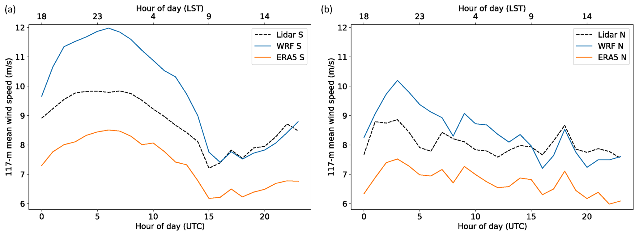
Figure 11Average diurnal cycle of the 117 m wind speed from lidar, WRF, and ERA-5 at the SGP C1 site for (a) southerly (112–196∘) and (b) northerly (315–45∘) wind flow.
3.6 Impact of surface fluxes at land-based sites
The ability of WTK-LED of accurately representing soil moisture could also contribute to explaining the overestimation of the diurnal cycle at SGP, as the variability of surface fluxes can change atmospheric turbulence and, as a consequence, drag (Geernaert, 1990). In Fig. 12, we compare the average diurnal cycle in sensible and latent heat fluxes from near-surface observations at SGP and from the WTK-LED. We find that WTK-LED overestimates the sensible heat flux during the day, while at night the WTK-LED prediction is, on average, quite accurate. The diurnal cycle of latent heat flux, on the other hand, is quite accurately modeled by WTK-LED throughout the day, on average, with a minor delay compared to the observed one. These results suggest that the exaggerated strong sensible heat flux by WTK-LED during the day (potentially caused by issues in the WTK-LED land use/land cover) is consistent with the WTK-LED's slight underprediction in the mean diurnal cycle of hub-height wind speed between 16:00–23:00 UTC, as a strong sensible heat flux would increase turbulence and drag. Soil moisture seems instead accurately modeled in WTK-LED given the relatively accurate latent heat flux values, so that the effects on the exaggerated diurnal cycle in hub-height wind speed are likely negligible Xia et al. (2021).

Figure 12Observed and WTK-LED-modeled average diurnal cycle of sensible and latent heat fluxes at the SGP site.
Accurate characterization of the wind resource aloft is a necessity for wind energy development. At land-based locations, direct observations of the wind resource at hub height are often challenging to collect due to a variety of reasons, including cost, complex topography, road access, and availability of electrical power. Offshore, collecting direct measurements of wind speeds aloft is even more challenging. Thus, NWP models and reanalysis products are often used to characterize the wind resource in the locations of interest for wind energy development.
Using 1 year of lidar data at both land-based and offshore test sites, we evaluate the WRF model as run in the WTK-LED setup and the ERA-5 reanalysis product in their wind resource assessment skills. To evaluate each data product, we calculate five model performance metrics – bias, cRMSE, r2, EMD, and a comparison between modeled and observed standard deviation. WTK-LED shows a smaller bias than ERA-5 at both the considered locations for all of the stability conditions. However, ERA-5 outperforms WTK-LED in terms of cRMSE for all stability cases both at the land-based and offshore sites. A potential explanation for this underperformance of WTK-LED in terms of cRMSE is WTK-LED's exaggeration of the average diurnal cycle at both sites but especially at the land-based one. In fact, when considering the diurnal variability of the WTK-LED bias, we find that WTK-LED generally shows a positive bias at night and more instances of negative biases during the daytime. At the land-based site, WTK-LED mostly overestimates the nighttime wind speed for southerly flow, when the location is impacted by wind plant wakes, which are not captured in WTK-LED. Additionally, the WTK-LED negative bias during the day is instead connected to an overestimation of the sensible heat flux at the site. On the other hand, ERA-5 is capable of well capturing the amplitude of the daily cycle in hub-height wind speed at the considered locations, albeit with a relatively constant negative bias throughout the diurnal cycle. Both WTK-LED and ERA-5 show high correlation offshore, while at the land-based site the correlation is marginally reduced, likely because of the increased complexity in modeling the wind flow in conjunction with topographic effects. Analysis at both locations shows ERA-5 having a slightly stronger correlation than WTK-LED. Based on the analysis of the EMD, the wind speed distributions predicted by WTK-LED better match the observed distributions compared to the ERA-5 data in all stability conditions. Also, WTK-LED better matches the observed standard deviation of wind speed at the offshore site, whereas WTK-LED and ERA-5 have a comparable performance at SGP.
Our results show how there is not a clear and universal winner between WRF (in the WTK-LED setup) and ERA-5 when assessing their skills for wind resource assessment at these two locations, offshore and flat terrain on land. However, when weighting the relative performance of the two data sources, it is worth noting how bias correction techniques have been successfully applied in the wind energy sector (Stoffelen, 1998; Costoya et al., 2020). With this in mind, we can expect that the worse ERA-5 performance in terms of bias would be easier to accommodate when compared to the WTK-LED underperformance in terms of random error (cRMSE) and correlation, with the caveat that observations of the wind resource, which might be challenging and/or expensive to obtain, are needed for a successful bias correction. On the other hand, it is worth emphasizing that WTK-LED offers data at a finer spatial and temporal resolution, which represents an essential advantage over reanalysis products for specific wind-energy-related applications, such as grid integration analyses (Archer et al., 2017), and in locations with complex terrain. Clearly, it is important to stress that our results are specific to the sites considered in the analysis, which are both characterized by simple topography. Future work can replicate our proposed validation in more complex terrain, where the coarser resolution of the reanalysis products is likely to have a severe negative impact on their skills in accurately representing the wind flow at hub height. Such analyses could provide additional understanding about why the WTK-LED WRF setup struggled, in our analysis, in well representing the wind speed diurnal cycle aloft. Finally, follow-on work will explore whether representing wind power plants in WRF improves the WRF performance in the vicinity of active wind power plants (e.g., by using the WRF wind farm parameterization, Fitch et al., 2012; Tomaszewski and Lundquist, 2020).
Observations at the SGP site are publicly available at https://doi.org/10.5439/1025186 (Newsom and Krishnamurthy, 2022). The NYSERDA lidar observations are publicly available at https://oswbuoysny.resourcepanorama.dnvgl.com (OceanTech Services/DNV GL, 2022). ERA-5 data are publicly available from the ECMWF's MARS archive. The WTK-LED data for the offshore domain are publicly available at https://doi.org/10.25984/1821404 (Bodini et al., 2021b). The WTK-LED data for the land-based site will be available to the public in the future. The open-source WRF model was used for the numerical weather prediction simulations.
The supplement related to this article is available online at: https://doi.org/10.5194/wes-7-487-2022-supplement.
NB, MO, PM, and JKL envisioned the analysis. MO ran the offshore WRF simulations. CD, AP, and EY ran the land-based WRF simulations. VP analyzed the data, in close consultation with NB and with general guidance from MO, PM, and JKL. VP and NB wrote the manuscript. All authors provided feedback on the paper draft.
At least one of the (co-)authors is a member of the editorial board of Wind Energy Science. The peer-review process was guided by an independent editor, and the authors also have no other competing interests to declare.
Publisher's note: Copernicus Publications remains neutral with regard to jurisdictional claims in published maps and institutional affiliations.
This research was performed using computational resources sponsored by the U.S. Department of Energy's Office of Energy Efficiency and Renewable Energy and located at the National Renewable Energy Laboratory.
This research has been supported by the U.S. Department of Energy Office of Energy Efficiency and Renewable Energy Wind Energy Technologies Office and by the National Offshore Wind Research and Development Consortium under agreement no. CRD-19-16351. This work was supported in part by the U.S. Department of Energy, Office of Science, Office of Workforce Development for Teachers and Scientists under the Science Undergraduate Laboratory Internship program.
This paper was edited by Andrea Hahmann and reviewed by two anonymous referees.
Al-Yahyai, S., Charabi, Y., and Gastli, A.: Review of the use of numerical weather prediction (NWP) models for wind energy assessment, Renew. Sust. Energ. Rev., 14, 3192–3198, https://doi.org/10.1016/j.rser.2010.07.001, 2010. a
Archer, C., Simão, H., Kempton, W., Powell, W. B., and Dvorak, M.: The challenge of integrating offshore wind power in the US electric grid. Part I: Wind forecast error, Renew. Energ., 103, 346–360, https://doi.org/10.1016/j.renene.2016.11.047, 2017. a
Babić, K., Bencetić Klaić, Z., and Večenaj, Ž.: Determining a turbulence averaging time scale by Fourier analysis for the nocturnal boundary layer, Geofizika, 29, 35–51, 2012. a
Bloomfield, H., Shaffrey, L., Hodges, K., and Vidale, P.: A critical assessment of the long-term changes in the wintertime surface Arctic Oscillation and Northern Hemisphere storminess in the ERA20C reanalysis, Environ. Res. Lett., 13, 094004, https://doi.org/10.1088/1748-9326/aad5c5, 2018. a
Bodini, N. and Optis, M.: The importance of round-robin validation when assessing machine-learning-based vertical extrapolation of wind speeds, Wind Energ. Sci., 5, 489–501, https://doi.org/10.5194/wes-5-489-2020, 2020. a
Bodini, N., Lundquist, J. K., and Kirincich, A.: US East Coast lidar measurements show offshore wind turbines will encounter very low atmospheric turbulence, Geophys. Res. Lett., 46, 5582–5591, https://doi.org/10.1029/2019GL082636, 2019. a, b
Bodini, N., Lundquist, J. K., and Kirincich, A.: Offshore wind turbines will encounter very low atmospheric turbulence, J. Phys. Conf. Ser., 1452, 012023, https://doi.org/10.1088/1742-6596/1452/1/012023, 2020. a
Bodini, N., Lundquist, J. K., and Moriarty, P.: Wind plants can impact long-term local atmospheric conditions, Sci. Rep.-UK, 11, 1–12, https://doi.org/10.1038/s41598-021-02089-2, 2021a. a, b, c
Bodini, N., Optis, M., Rossol, M., and Rybchuk, A.: National Renewable Energy Laboratory, US Offshore Wind Resource data for 2000–2019 [data set], https://doi.org/10.25984/1821404, 2021b. a
Brower, M.: Wind resource assessment: a practical guide to developing a wind project, John Wiley & Sons, ISBN 978-1-118-02232-0, 2012. a
Browning, K. and Wexler, R.: The determination of kinematic properties of a wind field using Doppler radar, J. Appl. Meteorol., 7, 105–113, https://doi.org/10.1175/1520-0450(1968)007<0105:TDOKPO>2.0.CO;2, 1968. a
Bureau of Ocean Energy Management: Outer Continental Shelf Renewable Energy Leases Map Book, Tech. rep., Bureau of Ocean Energy Management, https://www.boem.gov/sites/default/files/renewable-energy-program/Mapping-and-Data/Renewable_Energy_Leases_Map_Book_March_2019.pdf (last access: 1 March 2022), 2018. a
Bureau of Ocean Energy Management: Outer Continental Shelf Renewable Energy Leases Map Book, Tech. rep., https://www.boem.gov/sites/default/files/documents/oil-gas-energy/Renewable_Energy_Leases_Map_Book_March_2021_v2.pdf (last access: 1 March 2022), 2021. a, b
Carbon Trust Offshore Wind Accelerator: Carbon Trust Offshore Wind Accelerator Roadmap for the Commercial Acceptance of Floating LiDAR Technology, Tech. rep., Carbon Trust, https://prod-drupal-files.storage.googleapis.com/documents/resource/public/Roadmap%20for%20Commercial%20Acceptance%20of%20Floating%20LiDAR%20REPORT.pdf (last access: 1 March 2022), 2018. a
Compo, G. P., Whitaker, J. S., Sardeshmukh, P. D., Matsui, N., Allan, R. J., Yin, X., Gleason, B. E., Vose, R. S., Rutledge, G., Bessemoulin, P., Brönnimann, S., Brunet, M., Crouthamel, R. I., Grant, A. N., Groisman, P. Y., Jones, P. D., Kruk, M. C., Kruger, A. C., Marshall, G. J., Maugeri, M., Mok, H. Y., Nordli, Ø., Ross, T. F., Trigo, R. M., Wang, X. L., Woodruff, S. D., and Worley, S. J.: The twentieth century reanalysis project, Q. J. Roy. Meteor. Soc., 137, 1–28, https://doi.org/10.1002/qj.776, 2011. a
Costoya, X., Rocha, A., and Carvalho, D.: Using bias-correction to improve future projections of offshore wind energy resource: A case study on the Iberian Peninsula, Appl. Energ., 262, 114562, https://doi.org/10.1016/j.apenergy.2020.114562, 2020. a
De Franceschi, M. and Zardi, D.: Evaluation of cut-off frequency and correction of filter-induced phase lag and attenuation in eddy covariance analysis of turbulence data, Bound.-Lay. Meteorol., 108, 289–303, https://doi.org/10.1023/A:1024157310388, 2003. a
Dee, D. P., Uppala, S. M., Simmons, A. J., Berrisford, P., Poli, P., Kobayashi, S., Andrae, U., Balmaseda, M. A., Balsamo, G., Bauer, P., Bechtold, P., Beljaars, A. C. M., van de Berg, L., Bidlot, J., Bormann, N., Delsol, C., Dragani, R., Fuentes, M., Geer, A. J., Haimberger, L., Healy, S. B., Hersbach, H., Hólm, E. V., Isaksen, L., Kållberg, P., Köhler, M., Matricardi, M., McNally, A. P., Monge-Sanz, B. M., Morcrette, J.-J., Park, B.-K., Peubey, C., de Rosnay, P., Tavolato, C., Thépaut, J.-N., and Vitart, F.: The ERA-Interim reanalysis: Configuration and performance of the data assimilation system, Q. J. Roy. Meteor. Soc., 137, 553–597, https://doi.org/10.1002/qj.828, 2011. a
Dörenkämper, M., Olsen, B. T., Witha, B., Hahmann, A. N., Davis, N. N., Barcons, J., Ezber, Y., García-Bustamante, E., González-Rouco, J. F., Navarro, J., Sastre-Marugán, M., Sīle, T., Trei, W., Žagar, M., Badger, J., Gottschall, J., Sanz Rodrigo, J., and Mann, J.: The Making of the New European Wind Atlas – Part 2: Production and evaluation, Geosci. Model Dev., 13, 5079–5102, https://doi.org/10.5194/gmd-13-5079-2020, 2020. a, b, c
Draxl, C., Clifton, A., Hodge, B.-M., and McCaa, J.: The Wind Integration National Dataset (WIND) Toolkit, Appl. Energ., 151, 355–366, https://doi.org/10.1016/j.apenergy.2015.03.121, 2015. a, b, c
Fischer, M.: Carbon Dioxide Flux Measurement Systems (CO2FLX) Handbook, https://www.arm.gov/publications/tech_reports/handbooks/co2flx_handbook.pdf (last access 1 March 2022), 2004. a
Fitch, A. C., Olson, J. B., Lundquist, J. K., Dudhia, J., Gupta, A. K., Michalakes, J., and Barstad, I.: Local and mesoscale impacts of wind farms as parameterized in a mesoscale NWP model, Mon. Weather Rev., 140, 3017–3038, https://doi.org/10.1175/MWR-D-11-00352.1, 2012. a
Frehlich, R., Meillier, Y., Jensen, M. L., Balsley, B., and Sharman, R.: Measurements of boundary layer profiles in an urban environment, J. Appl. Meteorol. Clim., 45, 821–837, https://doi.org/10.1175/JAM2368.1, 2006. a
Geernaert, G.: Bulk parameterizations for the wind stress and heat fluxes, in: Surface waves and fluxes, Springer, 91–172, https://doi.org/10.1007/978-94-009-2069-9_5, 1990. a
Gelaro, R., McCarty, W., Suárez, M. J., Todling, R., Molod, A., Takacs, L., Randles, C. A., Darmenov, A., Bosilovich, M. G., Reichle, R., Wargan, K., Coy, L., Cullather, R., Draper, C., Akella, S., Buchard, V., Conaty, A., da Silva, A. M., Gu, W., Kim, G.-K., Koster, R., Lucchesi, R., Merkova, D., Nielsen, J. E., Partyka, G., Pawson, S., Putman, W., Rienecker, M., Schubert, S. D., Sienkiewicz, M., and Zhao, B.: The Modern-Era Retrospective Analysis for Research and Applications, version 2 (MERRA-2), J. Climate, 30, 5419–5454, https://doi.org/10.1175/JCLI-D-16-0758.1, 2017. a
Greene, S., McNabb, K., Zwilling, R., Morrissey, M., and Stadler, S.: Analysis of vertical wind shear in the Southern Great Plains and potential impacts on estimation of wind energy production, Int. J. Global Energy, 32, 191–211, https://doi.org/10.1504/IJGEI.2009.030651, 2009. a
Hahmann, A. N., Sīle, T., Witha, B., Davis, N. N., Dörenkämper, M., Ezber, Y., García-Bustamante, E., González-Rouco, J. F., Navarro, J., Olsen, B. T., and Söderberg, S.: The making of the New European Wind Atlas – Part 1: Model sensitivity, Geosci. Model Dev., 13, 5053–5078, https://doi.org/10.5194/gmd-13-5053-2020, 2020. a, b, c
Hallgren, C., Arnqvist, J., Ivanell, S., Körnich, H., Vakkari, V., and Sahlée, E.: Looking for an offshore low-level jet champion among recent reanalyses: a tight race over the Baltic Sea, Energies, 13, 3670, https://doi.org/10.3390/en13143670, 2020. a
Hersbach, H., Bell, B., Berrisford, P., Hirahara, S., Horányi, A., Muñoz-Sabater, J., Nicolas, J., Peubey, C., Radu, R., Schepers, D., Simmons, A., Soci, C., Abdalla, S., Abellan, X., Balsamo, G., Bechtold, P., Biavati, G., Bidlot, J., Bonavita, M., De Chiara, G., Dahlgren, P., Dee, D., Diamantakis, M., Dragani, R., Flemming, J., Forbes, R., Fuentes, M., Geer, A., Haimberger, L., Healy, S., Hogan, R. J., Hólm, E., Janisková, M., Keeley, S., Laloyaux, P., Lopez, P., Lupu, C., Radnoti, G., de Rosnay, P., Rozum, I., Vamborg, F., Villaume, S., and Thépaut, J.-N.: The ERA5 global reanalysis, Q. J. Roy. Meteor. Soc., 146, 1999–2049, https://doi.org/10.1002/qj.3803, 2020. a, b, c
Kalverla, P. C., Duncan Jr, J. B., Steeneveld, G.-J., and Holtslag, A. A. M.: Low-level jets over the North Sea based on ERA5 and observations: together they do better, Wind Energ. Sci., 4, 193–209, https://doi.org/10.5194/wes-4-193-2019, 2019. a
King, J., Clifton, A., and Hodge, B.-M.: Validation of power output for the WIND Toolkit, Tech. rep., National Renewable Energy Lab. (NREL), Golden, CO (United States), https://doi.org/10.2172/1159354, 2014. a
Kubik, M., Brayshaw, D. J., Coker, P. J., and Barlow, J. F.: Exploring the role of reanalysis data in simulating regional wind generation variability over Northern Ireland, Renew. Energ., 57, 558–561, https://doi.org/10.1016/j.renene.2013.02.012, 2013. a
Lieberman-Cribbin, W., Draxl, C., and Clifton, A.: Guide to using the WIND toolkit validation code, Tech. rep., National Renewable Energy Lab. (NREL), Golden, CO (United States), https://doi.org/10.2172/1166659, 2014. a
Livingston, H. G. and Lundquist, J. K.: How many offshore wind turbines does New England need?, Meteorol. Appl., 27, e1969, https://doi.org/10.1002/met.1969, 2020. a
Molina, M., Gutiérrez, C., and Sánchez, E.: Comparison of ERA5 surface wind speed climatologies over Europe with observations from the HadISD dataset, Int. J. Climatol., 41, 4864–4878, https://doi.org/10.1002/joc.7103, 2021. a
Moriarty, P., Hamilton, N., Debnath, M., Fao, R., Roadman, J., van Dam, J., Herges, T., Isom, B., Lundquist, J., Maniaci, D., Naughton, B., Pauly, R., Roadman, J., Shaw, W., van Dam, J., and Wharton, S.: American WAKe ExperimeNt (AWAKEN), Tech. rep., National Renewable Energy Lab. (NREL), Golden, CO (United States), https://www.nrel.gov/docs/fy20osti/75789.pdf (last access: 1 March 2022), 2020. a
Musial, W., Heimiller, D., Beiter, P., Scott, G., and Draxl, C.: Offshore wind energy resource assessment for the United States, Tech. rep., National Renewable Energy Laboratory (NREL), Golden, CO (United States), https://doi.org/10.2172/1324533, https://www.nrel.gov/docs/fy16osti/66599.pdf (last access: 1 March 2022), 2016. a
Newsom, R. and Krishnamurthy, R.: Doppler lidar (DL) handbook, Tech. rep., DOE Office of Science Atmospheric Radiation Measurement (ARM) Program, https://www.arm.gov/publications/tech_reports/handbooks/dl_handbook.pdf (last access: 1 March 2022), 2012. a
Newsom, R. and Krishnamurthy, R.: Doppler Lidar (DLPPI), Atmospheric Radiation Measurement (ARM) user facility [data set], https://doi.org/10.5439/1025186, 2022. a
OceanTech Services/DNV GL: NYSERDA Floating Lidar Buoy Data, https://oswbuoysny.resourcepanorama.dnvgl.com, last access: 1 March 2022. a, b, c
Optis, M., Rybchuk, O., Bodini, N., Rossol, M., and Musial, W.: 2020 Offshore Wind Resource Assessment for the California Pacific Outer Continental Shelf, Tech. rep., National Renewable Energy Lab. (NREL), Golden, CO (United States), https://doi.org/10.2172/1677466, 2020. a
Ramon, J., Lledo, L., Torralba, V., Soret, A., and Doblas-Reyes, F. J.: What global reanalysis best represents near-surface winds?, Q. J. Roy. Meteor. Soc., 145, 3236–3251, https://doi.org/10.1002/qj.3616, 2019. a
Rose, S. and Apt, J.: What can reanalysis data tell us about wind power?, Renew. Energ., 83, 963–969, https://doi.org/10.1016/j.renene.2015.05.027, 2015. a
Rybchuk, A., Optis, M., Lundquist, J. K., Rossol, M., and Musial, W.: A Twenty-Year Analysis of Winds in California for Offshore Wind Energy Production Using WRF v4.1.2, Geosci. Model Dev. Discuss. [preprint], https://doi.org/10.5194/gmd-2021-50, 2021. a
Schwartz, M., George, R., and Elliott, D.: The use of reanalysis data for wind resource assessment at the National Renewable Energy Laboratory, Tech. rep., National Renewable Energy Lab., Golden, CO (US), https://www.osti.gov/biblio/10425 (last access: 1 March 2022), 1999. a
Sheridan, L. M., Krishnamurthy, R., Gorton, A. M., Shaw, W. J., and Newsom, R. K.: Validation of Reanalysis-Based Offshore Wind Resource Characterization Using Lidar Buoy Observations, Mar. Technol. Soc. J., 54, 44–61, https://doi.org/10.4031/MTSJ.54.6.13, 2020. a, b
Skamarock, W. C., Klemp, J. B., Dudhia, J., Gill, D. O., Barker, D. M., Duda, M. G., Huang, X.-Y., Wang, W., and Powers, J. G.: A description of the advanced research WRF model version 4, National Center for Atmospheric Research, Boulder, CO, USA, 145, https://doi.org/10.5065/D68S4MVH, 2019. a
Smith, E. N., Gibbs, J. A., Fedorovich, E., and Klein, P. M.: WRF Model study of the Great Plains low-level jet: Effects of grid spacing and boundary layer parameterization, J. Appl. Meteorol. Clim., 57, 2375–2397, https://doi.org/10.1175/JAMC-D-17-0361.1, 2018. a
Smith, E. N., Gebauer, J. G., Klein, P. M., Fedorovich, E., and Gibbs, J. A.: The Great Plains low-level jet during PECAN: Observed and simulated characteristics, Mon. Weather Rev., 147, 1845–1869, https://doi.org/10.1175/MWR-D-18-0293.1, 2019. a
Soares, P. M., Lima, D. C., and Nogueira, M.: Global offshore wind energy resources using the new ERA-5 reanalysis, Environ. Res. Lett., 15, 1040a2, https://doi.org/10.1088/1748-9326/abb10d, 2020. a
Song, J., Liao, K., Coulter, R. L., and Lesht, B. M.: Climatology of the low-level jet at the southern Great Plains atmospheric boundary layer experiments site, J. Appl. Meteorol., 44, 1593–1606, https://doi.org/10.1175/JAM2294.1, 2005. a
Stoffelen, A.: Toward the true near-surface wind speed: Error modeling and calibration using triple collocation, J. Geophys. Res.-Oceans, 103, 7755–7766, https://doi.org/10.1029/97JC03180, 1998. a
Taylor, K. E.: Summarizing multiple aspects of model performance in a single diagram, J. Geophys. Res.-Atmos., 106, 7183–7192, https://doi.org/10.1029/2000JD900719, 2001. a
Tomaszewski, J. M. and Lundquist, J. K.: Simulated wind farm wake sensitivity to configuration choices in the Weather Research and Forecasting model version 3.8.1, Geosci. Model Dev., 13, 2645–2662, https://doi.org/10.5194/gmd-13-2645-2020, 2020. a
Vaseršte\ĭn, L. N.: On the stabilization of the general linear group over a ring, Mathematics of the USSR-Sbornik, 8, 383, 1969. a
Webb, E. K., Pearman, G. I., and Leuning, R.: Correction of flux measurements for density effects due to heat and water vapour transfer, Q. J. Roy. Meteor. Soc., 106, 85–100, https://doi.org/10.1002/qj.49710644707, 1980. a
Xia, G., Draxl, C., Berg, L. K., and Cook, D.: Quantifying the Impacts of Land Surface Modeling on Hub-Height Wind Speed under Different Soil Conditions, Mon. Weather Rev., 149, 3101–3118, https://doi.org/10.1175/MWR-D-20-0363.1, 2021. a
Zheng, C.-w., Xiao, Z.-n., Peng, Y.-h., Li, C.-y., and Du, Z.-b.: Rezoning global offshore wind energy resources, Renew. Energ., 129, 1–11, https://doi.org/10.1016/j.renene.2018.05.090, 2018. a