Efficient Bayesian calibration of aerodynamic wind turbine models using surrogate modeling

This paper presents an efficient strategy for the Bayesian calibration of parameters of aerodynamic wind turbine models. The strategy relies on constructing a surrogate model (based on adaptive polynomial chaos expansions), which is used to perform both parameter selection using global sensitivity analysis and parameter calibration with Bayesian inference. The effectiveness of this approach is shown in two test cases: calibration of airfoil polars based on the measurements from the DANAERO MW experiments and calibration of five yaw model parameters based on measurements on the New MEXICO turbine in yawed conditions. In both cases, the calibrated models yield results much closer to the measurement data, and in addition they are equipped with an estimate of the uncertainty in the predictions.

1 Introduction

Aeroelastic wind turbine models based on blade element momentum theory (BEM) are used extensively within the wind energy community for simulating rotor characteristics such as aerodynamic loads, power, and thrust. They are indispensable tools for the design and optimization of wind turbines. However, in several situations, the accuracy of such models can be unsatisfactory when comparing the results of the model predictions with experiments (Buhl and Manjock, 2006). For instance, the “blind comparison” study organized by NREL (Simms et al., 2001) revealed large differences when comparing the predictions of different aeroelastic models with experimental measurements. In some cases, differences exceeded 200 %, even when simple operating conditions were being considered (i.e., uniform wind speed, fixed blade pitch, and zero yaw angle). The differences were attributed to the several empirical correction factors or tuning parameters integrated into the aeroelastic models that are used to improve the unsteady aerodynamic and aeroelastic force predictions. More recent results show better agreements, at least for simple wind tunnel conditions, but many challenges exist, for example in dynamic wake prediction and yaw, especially in the context of upscaling (see Schepers et al., 2021, chap. 12). Examples are dynamic wake correction factors or dynamic stall model parameters (Wang et al., 2016). These empirical correction factors suffer from inherent uncertainties. As explained by Leishman (2002) and Sørensen and Toft (2010), a major challenge is to identify the uncertainties associated with wind turbine aerodynamics in order to develop more rigorous models suitable for a wider range of operating conditions, as well as to better integrate and validate these models with reference to good-quality experimental measurements. Similarly, Abdallah et al. (2015) concluded that the uncertainties in the model parameters used in aeroelastic models have a significant impact on the accuracy of model predictions. In other words, in order to build robust aeroelastic wind turbine models with a quantified level of uncertainty, it is important to calibrate these models in a framework that includes uncertainty estimates (Murcia, 2016).

A common approach to calibrate aerodynamic models is via parameter tuning, in which one assumes that the form of the model is in principle correct and that the errors in the model outcomes can be reduced by properly choosing the value of one or more parameters. These parameter values are preferably independent of the model inputs; i.e., they should lead to accurate predictions for a wide range of operating conditions. Examples of parametric model calibration in wind energy applications can be found in Bottasso et al. (2014), Murcia et al. (2018), and van Beek et al. (2021). In these calibration studies, either least-squares methods or maximum likelihood estimation (MLE) methods are used. MLE determines the model parameters such that it maximizes the likelihood that describes the (presumed) relation between model and measurement data (Severini, 2000). However, a major drawback of least-squares and MLE methods is that prior information is not naturally included (Smith, 2013). Using prior information is especially relevant when few measurement data are available, which is a common situation in wind turbine model calibration (van Kuik et al., 2016). Consequently, the MLE method can exhibit large uncertainty in the estimation of the parameters and, as a result, in the model predictions. Furthermore, in least-squares or MLE methods, parameters are typically considered deterministic (fixed but unknown) so that a point estimate (plus confidence intervals) results, which does not provide details regarding the full probability distribution of the calibrated parameters (Smith, 2013).

In order to address these issues, the goal of this paper is to set up a framework for calibrating aerodynamic wind turbine models that also works in case of limited measurement data and gives full uncertainty estimates (in terms of probability density functions) of the calibrated parameters. We propose a rigorous approach to the calibration problem by recasting it in a probabilistic setting using a Bayesian framework (Kennedy and O'Hagan, 2001). Within this framework, the model parameters are posed as random variables, and it is possible to include prior knowledge by specifying a prior distribution, thus allowing model calibration even when small sample sizes are available. Bayes' theorem (Bayes, 1763) is then used to calculate the posterior distribution of the model parameters conditioned on the given measurement data. The posterior distribution gives more information than MLE about the calibrated parameters; i.e., it gives the entire posterior probability density function, from which point estimates such as the posterior mean and the standard deviation can be calculated (if required). Furthermore, the calibration can be verified by computing the posterior predictive distribution (Gelman et al., 2013). Since the expression for the posterior distribution is generally not available in an analytically tractable form (Gelman et al., 2013), we will resort to Markov chain Monte Carlo (MCMC) methods to sample from the posterior distribution (Papageorgiou and Traub, 1996; Andrieu et al., 2003). The main downside of the Bayesian approach, associated with the MCMC sampling step, is its high computational expense. We will alleviate this issue by constructing a surrogate model of the full aerodynamic model (Sudret, 2008) and perform the MCMC sampling with the surrogate model in lieu of the full model. In this work, polynomial chaos expansions (PCEs) (Laloy et al., 2013) will be used, which can be constructed using a relatively small number of aerodynamic model runs.

In addition, the cost of the Bayesian calibration can be reduced by eliminating non-influential parameters. These can be determined by performing a sensitivity analysis (Oakley and O'Hagan, 2004). In this study we will employ a variance-based global sensitivity analysis using Sobol' indices (Sobol', 2001), based on our earlier work (Kumar et al., 2020). Determining Sobol' indices is straightforward once the PCE surrogate model has been determined.

The novelty of this work lies in the construction of a Bayesian framework for aerodynamic wind turbine model calibration. In addition to that, two realistic calibration studies based on the DANAERO MW experiments (Madsen et al., 2010) and the New MEXICO experimental data (Boorsma and Schepers, 2016) were performed. The former dataset will be used to calibrate airfoil polars, while the latter will be used to calibrate yaw model parameters. The DANAERO experiments were supplied by DTU within the framework of IEA Task 29. Although extensive comparisons between results from a large variety of codes (including the Aero-Module employed in this study) were performed on DANAERO and New MEXICO in Task 29 (Schepers et al., 2018, 2021), no thorough uncertainty analysis and calibration were performed yet. We stress that, even though these studies show a realistic application of our method with actual data, they correspond to idealized situations, and the main purpose of this paper is to demonstrate the calibration framework and its potential for application to a wide variety of wind engineering problems.

The outline of this paper is as follows: Sect. 2 discusses the two experimental datasets considered in this study (DANAERO and New MEXICO). Section 3 describes the aerodynamic code used in this work (the so-called Aero-Module) plus parametrization of its inputs and outputs. The Bayesian calibration methodology, which is accelerated by constructing a PCE-based surrogate model, is detailed in Sect. 4. Finally, the results of the calibration and discussion are presented in Sect. 5 followed by conclusions drawn in Sect. 6.

2 Experimental data description

In order to demonstrate the proposed Bayesian calibration framework, measurements from two experiments constitute the basis for the analysis, which are explained in Sect. 2.1 and 2.2.

2.1 DANAERO MW experiment

The objective of the DANAERO MW experiment was to provide an experimental basis that can improve the understanding of the fundamental aerodynamic and aeroacoustic phenomena using a full-scale wind turbine model (Madsen et al., 2010). A 2.3 MW NM80 turbine located at the Tjæreborg Enge site and a nearby met mast were both instrumented with various sensors. A LM38.8 m test blade (schematic) instrumented with pressure taps at four blade sections is shown in Fig. 1 (left). The data acquisition rate was 35 Hz, and in total about 275 10 min time series were acquired between July and September 2009, which were made available for the present analysis.

Figure 1 Schematic of NM80 wind turbine blade implemented with surface pressure taps (left) and NACA 63-418 airfoil blade section tested in the LM Wind Power wind tunnel in Lunderskov (right) (Özçakmak et al., 2018).

In the current study, we aim to calibrate airfoil polars (to be described later), and only a subset of the entire DANAERO dataset will be used. To be precise, data from “Run 14” (a single 10 min time series) on the first measurement day (16 July 2009) is used. This corresponds to a case with little yaw and shear and with little turbulence (roughly constant inflow conditions) under normal operation. The inflow velocity for this case is around 6 m s⁻¹, and the rotational speed is 12 rpm. Within this particular 10 min series, the data corresponding to $\mathrm{200}\text{s}<t<\mathrm{450}\text{s}$ were used, in which almost constant wind and rotor speed were observed. For more details, we refer to Madsen et al. (2018). As a result, we have normal force measurements y^(ϱ)(t) at the four blade sections ($\mathit{\varrho }=\mathrm{1},\mathrm{2},\mathrm{3},\mathrm{4}$) at N_t=8750 discrete time steps, gathered in the data matrix y:

$$\begin{array}{}\text{(1)}& \mathbf{y}=\left(\begin{array}{ccc}{y}^{\left(\mathrm{1}\right)}\left(t_{\mathrm{1}}\right)& \mathrm{\cdots }& y^{\left(\mathrm{1}\right)}\left(t_{N_t}\right)\\ \mathrm{⋮}& & \mathrm{⋮}\\ y^{\left(\mathrm{4}\right)}\left(t_{\mathrm{1}}\right)& \mathrm{\cdots }& y^{\left(\mathrm{4}\right)}\left(t_{N_t}\right)\end{array}\right),\end{array}$$

where t_j = $j\mathit{\tau }/N_t$ and τ = 250 s. The radial positions (measured from the center of the hub) corresponding to these sections are $r=(\mathrm{13.116},\mathrm{19.06},\mathrm{30.216},\mathrm{36.775})\text{m}$; see Fig. 1 (left). To obtain the distance from the blade root, as used in the Aero-Module calculations, we subtract the distance from the blade root to the hub center, which is 1.24 m. Although using a single 10 min time series corresponding to a single operating condition is generally insufficient to perform accurate BEM model calibration, this experiment is merely used as a first demonstration of our framework. A more advanced calibration run involving multiple operating conditions will be performed with the data from the New MEXICO experiment described in the next section.

Besides the data obtained directly from the Tjæreborg Enge site, airfoil polars were obtained from several wind tunnel tests, such as those on the NACA 63-418 airfoil cross-section in the LM Wind Power wind tunnel (Madsen et al., 2010); see Fig. 1 (right). These airfoil polars consist of lift, drag, and moment coefficients as a function of angle of attack. Four polars are used in this study, whose location roughly (but not exactly) corresponds to the measurement positions mentioned above. These polars will form the inputs to our BEM code (see Sect. 3.1) and are to be calibrated in this study.

2.2 New MEXICO experiment

The main objective of the New MEXICO experimental campaign was to create a database of detailed aerodynamic and load measurements on an experimental wind turbine to be used for computational model validation and improvement (Boorsma and Schepers, 2014, 2016). To this aim, a three-bladed 4.5 m diameter wind turbine model was built and tested in the large low-speed facility of the German–Dutch wind tunnel (DNW-LLF) during a campaign in June–July 2014 (see Fig. 2); a detailed description of the experiment is available in Boorsma and Schepers (2014). The data acquisition system consists of dynamic pressure sensors divided over five sections and distributed over three blades: at 25 % and 35 % (blade 1), 60 % (blade 2), and 82 % and 92 % (blade 3) radial position, respectively. These were post-processed to obtain (amongst others) sectional normal forces, whose variations with azimuth and yaw angle will be considered in this study.

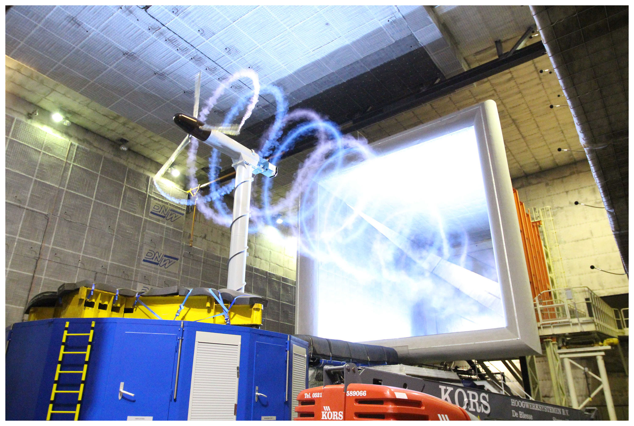
Figure 2 New MEXICO rotor tested in the DNW-LLF wind tunnel (Boorsma and Schepers, 2014, 2016).

The corresponding operating conditions (scenarios) are described by a vector 𝒮_i:

$$\begin{array}{}\text{(2)}& {\mathcal{S}}_i=({\mathit{\rho }}_{\mathrm{\infty }},V_{\mathrm{\infty }},\mathit{\beta },\mathit{\varphi }),i=\mathrm{1},\mathrm{\dots },N_S,\end{array}$$

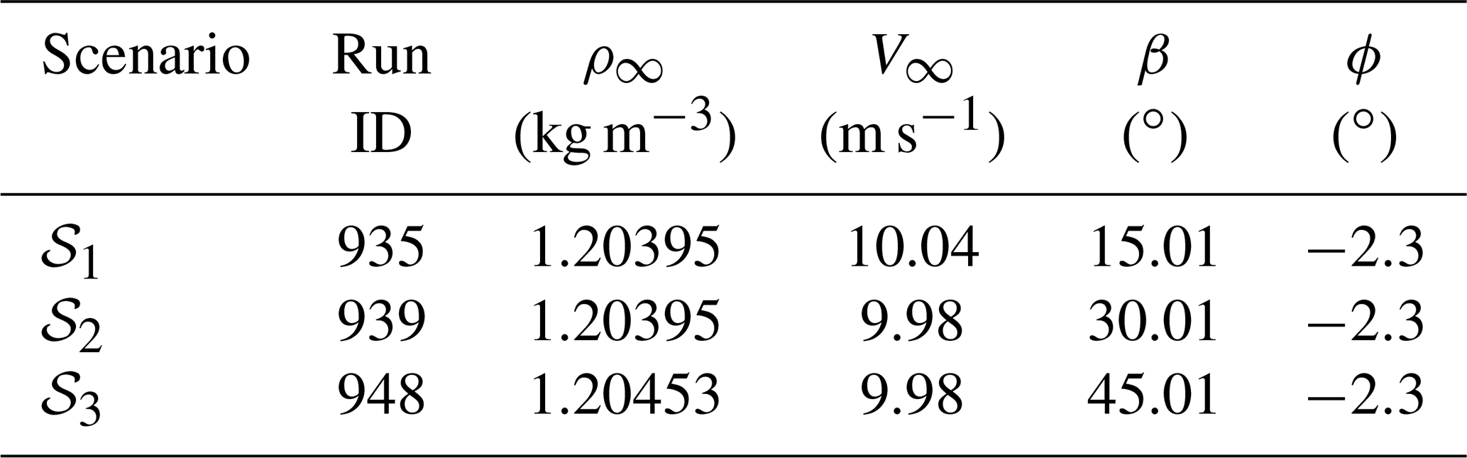
where ρ_∞ is the density, V_∞ is the inflow velocity, β is the yaw angle, ϕ is the pitch angle, and N_S is the number of operating conditions. For the yawed flow case, 29 runs were performed in total, but in this study we restrict ourselves to N_S=3, corresponding to IDs 935, 939, and 948 (see Table 1). These conditions are such that a significant induced velocity is expected (so that the yaw model will have a significant effect), while at the same time there is little dynamic stall occurring. For each operating condition, there is a corresponding dataset containing the normal force as a function of azimuth at five radial sections $\mathit{\varrho }=\mathrm{1},\mathrm{\dots },\mathrm{5}$ (the tangential force is also available but not used here due to the large uncertainty associated with the measurements). Similar to Eq. (1), this will be denoted by the data matrix y but now with an additional subscript i to indicate that there is a data matrix corresponding to each different operating condition:

$$\begin{array}{}\text{(3)}& {\mathbf{y}}_i={\left(\begin{array}{ccc}{y}^{\left(\mathrm{1}\right)}\left(t_{\mathrm{1}}\right)& \mathrm{\cdots }& y^{\left(\mathrm{1}\right)}\left(t_{N_t}\right)\\ \mathrm{⋮}& & \mathrm{⋮}\\ y^{\left(\mathrm{5}\right)}\left(t_{\mathrm{1}}\right)& \mathrm{\cdots }& y^{\left(\mathrm{5}\right)}\left(t_{N_t}\right)\end{array}\right)}_i,i=\mathrm{1},\mathrm{\dots },N_S.\end{array}$$

Table 1 New MEXICO operating conditions considered for yaw model calibration.

3 Aerodynamic wind-turbine model

3.1 Aero-Module description and uncertainties

TNO (Netherlands Organisation for Applied Scientific Research) is the developer of a state-of-the-art aerodynamic model based on a BEM formulation, called the Aero-Module (Boorsma and Grasso, 2015) (formerly developed by ECN, now part of TNO). The model simulates the aerodynamic behavior of wind turbines by combining the concept of momentum conservation of the flow (BEM theory) and can be coupled to an aeroelastic model that solves the equations of motion for the structure, possibly extended with the hydrodynamics of the sea and control algorithms. In this work, we concentrate on the first aspect, namely the prediction of flow and blade forces as given by the BEM method. All calculations are done for a rigid construction, since the effects from flexibilities are considered small: in New Mexico a small rigid rotor was used, and for DANAERO the elastic effects were found to be small (Schepers et al., 2021). A detailed description of the BEM approach within the Aero-Module is beyond the scope of the current discussion and can be found in Boorsma et al. (2012). Important for the current discussion is to distinguish between different types of inputs in the Aero-Module. The first type of inputs consists of external (operating) conditions, such as wind speed and air density. The second type consists of turbine specifications, such as the blade geometry. The third type consists of model parameters inherent to the BEM formulation, such as lift and drag polars, tip correction factors, and yaw model parameters. For the case of a rigid turbine, with a uniform inflow field, the main uncertainties in this third type (the BEM model parameters) mainly arise from the following (Abdallah et al., 2015).

• Airfoil aerodynamics. The static airfoil data from wind tunnel experiments or from 2D airfoil codes, utilized as an input for the BEM simulations, have significant uncertainties and can be inaccurate (Bak et al., 2010).

• Empirical models. Several empirical models such as dynamic stall models, 3D correction models, and Prandtl correction models are used to include unsteady and 3D effects in BEM models (Wang et al., 2016; Schepers, 2012). It is often the choice of a designer to select between different empirical models, which can suffer from modeling uncertainty.

In the current study we will focus on calibrating this third type of input parameters, i.e., the model parameters, in particular static airfoil data (lift, drag, and moment polars) and yaw model parameters. However, we stress that the calibration framework that is presented here can be directly applied to the first and second type of uncertainties as well.

In mathematical notation, these uncertainties will be captured in a vector of model parameters ${\mathit{\theta }}_{\mathrm{M}}=({\mathit{\theta }}_{\mathrm{M},\mathrm{1}},\mathrm{\dots },{\mathit{\theta }}_{\mathrm{M},{\mathrm{N}}_{\mathit{\theta }}})\in {\mathbb{R}}^{N_{\mathit{\theta }}}$, to be described in more detail in Sect. 3.2. The Aero-Module for a certain wind turbine is denoted by ℳ and returns a vector of outputs Y, depending on the (uncertain) model parameters θ_M and on the (given) value of the operating conditions 𝒮_i:

$$\begin{array}{}\text{(4)}& Y_i=Y_i\left({\mathit{\theta }}_{\mathrm{M}}\right)=\mathcal{M}({\mathit{\theta }}_{\mathrm{M}},{\mathcal{S}}_i),i=\mathrm{1},\mathrm{\dots },N_S,\end{array}$$

where N_S is the number of operating conditions. The output Y contains, amongst others forces, moments and power, which are generally time-dependent. Typically only a subset of the entire Aero-Module output, indicated as the quantity of interest Q, will be used to perform sensitivity analysis and calibration of the model. This will be further described in Sect. 3.3. It should be stressed that θ_M, Y, and Q are random vectors, each of which is associated with a joint probability density function.

Figure 3 Flowchart for our Bayesian calibration framework.

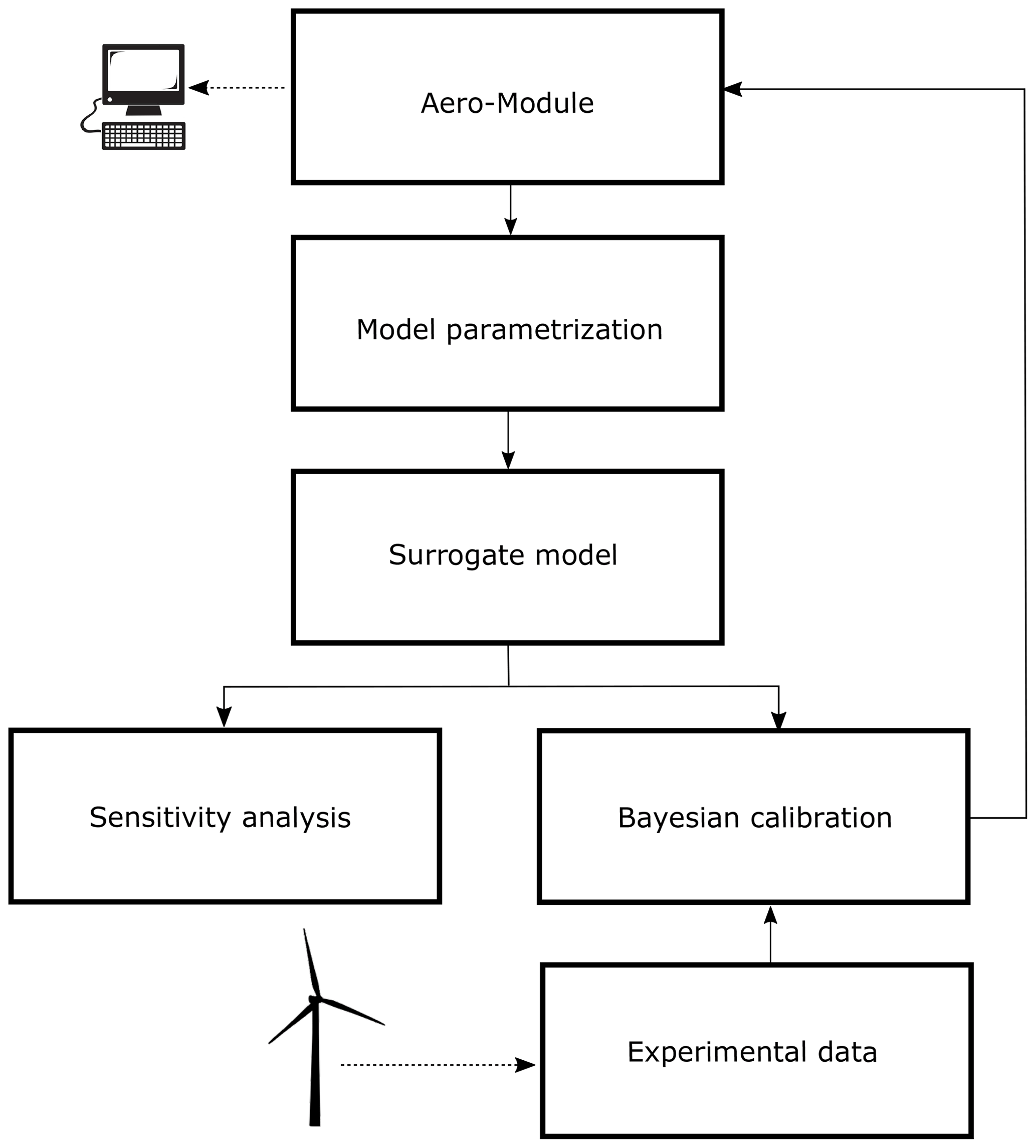
The analysis carried out in this study is based on the procedure shown in Fig. 3, including the steps that will be separately described in the following sub-sections. The proposed Bayesian calibration approach is performed using the UQLab uncertainty quantification software (Marelli and Sudret, 2014), especially the recently developed Bayesian inversion module (Wagner et al., 2022).

3.2 Input parametrization

3.2.1 DANAERO case: uncertainty in polars

For the DANAERO case, we will consider the uncertainties associated with the airfoil aerodynamics: lift coefficient (C_l), drag coefficient (C_d), and moment coefficient (C_m). These coefficients are functions of both angle of attack α and radial position r along the blade (also Reynolds number and Mach number, but this dependence is not studied here); this gives rise to a very large number of uncertain parameters. In order to reduce this number, we parametrize these uncertainties as a function of angle of attack and radial position.

The parametrization as a function of radial position is automatically accounted for within the Aero-Module code: the user has to provide the lift, drag, and moment polars only for a few airfoil sections along the radius of the blade, e.g., C_l, j(α) for j=1…N_sec, with N_sec being the number of airfoil sections. The Aero-Module interpolates these polars to other radial positions based on the relative airfoil thickness.

The parametrization as a function of angle of attack is performed as follows. Given a reference polar, e.g., $C_{\mathrm{l},\text{ref},j}\left(\mathit{\alpha }\right)$ for the lift coefficient at airfoil section j, a perturbed polar ${\stackrel{\mathrm{̃}}{C}}_{\mathrm{l},j}$ is obtained by scaling the reference curve as follows:

$$\begin{array}{}\text{(5)}& \begin{array}{rl}& {\stackrel{\mathrm{̃}}{C}}_{\mathrm{l},j}\left(\mathit{\alpha }\right)=\\ & \left\{\begin{array}{ll}{C}_{\mathrm{l},\text{ref},j}\left(\mathit{\alpha }\right)\cdot (\mathrm{1}+\mathrm{\Delta }{C}_{\mathrm{l},j})& {\mathit{\alpha }}_{\text{min},j}<\mathit{\alpha }<{\mathit{\alpha }}_{\text{max},j},\\ C_{\mathrm{l},\text{ref},j}\left(\mathit{\alpha }\right)& \text{otherwise}.\end{array}\right.\end{array}\end{array}$$

The same equation is used for the drag and moment coefficients. The value of ΔC_l, j determines how much the reference curve is scaled. The bounds α_min,j and α_max,j indicate for each airfoil section j which part of the polar is perturbed. The unperturbed and perturbed parts of the polar are combined via a non-uniform rational basis spline (NURBS) curve. A similar equation holds for the drag and moment coefficients. Example curves obtained with different realizations of ΔC_l, ΔC_d, and ΔC_m are shown in Fig. 4.

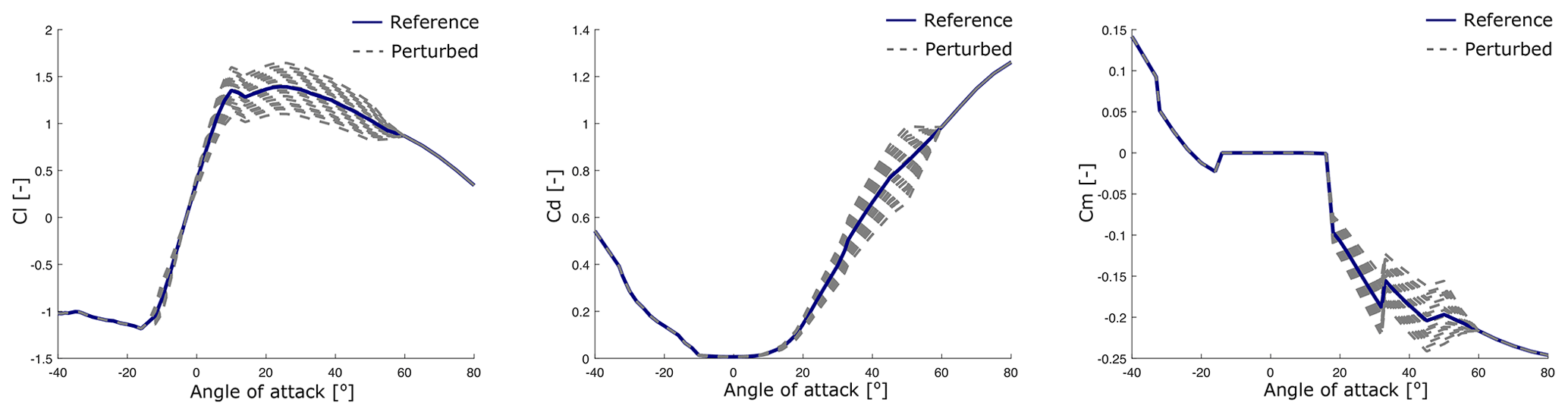
Figure 4 Examples of perturbed C_l, C_d, and C_m polars at Sect. 2 as described by Eq. (5), with ${\mathit{\alpha }}_{\text{min}}=-\mathrm{10}{}^{\circ }$ and ${\mathit{\alpha }}_{\text{max}}=\mathrm{50}{}^{\circ }$.

For the DANAERO case, where the number of airfoil sections is N_sec=4, the parametrization of lift, drag, and moment coefficients leads to the following N_θ=12-dimensional parameter vector θ_M:

$$\begin{array}{}\text{(6)}& \begin{array}{rl}{\mathit{\theta }}_{\mathrm{M}}& =(\mathrm{\Delta }{C}_{\mathrm{l},\mathrm{1}},\mathrm{\dots },\mathrm{\Delta }{C}_{\mathrm{l},\mathrm{4}},\mathrm{\Delta }{C}_{\mathrm{d},\mathrm{1}},\mathrm{\dots },\mathrm{\Delta }{C}_{\mathrm{d},\mathrm{4}},\mathrm{\Delta }{C}_{\mathrm{m},\mathrm{1}},\\ & \mathrm{\dots },\mathrm{\Delta }{C}_{\mathrm{m},\mathrm{4}}).\end{array}\end{array}$$

One advantage of the multiplicative type of parametrization Eq. (5) is that the uncertainty becomes largest when the magnitude of the reference curve is large; this is physically meaningful, as lift curves tend to be most uncertain around the region of maximum lift (and/or at high angles of attack, but these are not considered here). However, other types of parametrization could be considered. For example, Bottasso et al. (2014) considered an additive type of correction (i.e., $C_{\mathrm{l},\text{ref}}+\mathrm{\Delta }{C}_{\mathrm{l}}$), with ΔC_l expressed in terms of shape functions and coefficients, and applied a decorrelation procedure to improve the identifiability of the drag coefficients. Matthäus et al. (2017) obtained a perturbed lift curve by interpolating between two reference lift curves corresponding to clean and rough states. In Abdallah et al. (2015), a number of typical points along the C_l(α) curve (e.g., maximum lift, separation point) was used to construct a parametric spline approximation to the lift curve. Since the focus of this article lies in showing how the combination of surrogate models, sensitivity analysis, and Bayesian inference can be used for efficient calibration, we have not considered such more advanced polar parametrizations, but we note that it is possible to use any of them within our calibration framework.

3.2.2 New MEXICO case: uncertainty in yaw model

With the New MEXICO experiments, as described in Sect. 2.2, the goal is to calibrate a set of parameters that determine the yaw model of the Aero-Module. This yaw model is described in Schepers (2012) and consists of 10 amplitude coefficients denoted by AM_kl and 10 phase coefficients denoted by PH_kl ($k=\mathrm{1},\mathrm{2}$; l=1 … 5), which are used in an equation for the induced velocity in yawed conditions (see Eq. C1 in Appendix C). We will (as a proof of concept) calibrate only the first five parameters of this model; i.e., we take

$$\begin{array}{}\text{(7)}& {\mathit{\theta }}_{\mathrm{M}}=({\text{AM}}_{\mathrm{11}},{\text{AM}}_{\mathrm{12}},{\text{AM}}_{\mathrm{13}},{\text{AM}}_{\mathrm{14}},{\text{AM}}_{\mathrm{15}}).\end{array}$$

The nominal values for these coefficients can be found in Appendix B in Schepers (2012) and are repeated in Appendix C. The other yaw model parameters are associated with the phase shift of the induced velocity and with higher-order harmonics and will be left at their nominal values, since the number of experimental data considered here is too limited to perform a sensible calibration.

3.3 Output parametrization and quantity of interest

The Aero-Module predictions given by Eq. (4) involve a large set of time-dependent quantities, making the dimension of the output effectively very high dimensional. For the purpose of sensitivity analysis and model calibration, it is highly desirable to reduce the dimensionality of the output. As a first step (both for DANAERO and New MEXICO simulations), out of all possible outputs (forces, moments, power, etc.) we restrict ourselves to the normal forces F_N (“normal” indicating normal to the chord), interpolated to the radial positions corresponding to the measurement positions.

3.3.1 DANAERO case: time-independent results

For the DANAERO case, the inflow conditions in the Aero-Module are assumed constant in time, and given that there is no shear or yaw, this results in normal force predictions that are steady state (time-independent). The experimental data are, on the other hand, only approximately steady state since they were performed in atmospheric conditions. The question then arises of how to perform the comparison between simulation and experiment in order to perform the desired calibration. The most natural possibility would probably be to average the experimental data in time. However, since we have only a single 10 min time series at this condition, this would effectively reduce the number of measurement points to just a single point, which would be too little to perform any sensible calibration. As a compromise, we decided to split the time series into a number of subsets (10, 50, 100, and 200) of the 8750 data points mentioned in Eq. (1), at regularly spaced intervals. The mean of each subset is then considered to be an independent measurement point that will be used in the calibration process (as if they were corresponding to different measurements). This approach allows us to clearly show the effect of increasing the number of measurement points on the convergence of the posterior distribution of the airfoil polars. This will be further detailed in Sect. 5.1.

3.3.2 New Mexico case: time-dependent results

For the New MEXICO case, the operating conditions lead to results that are periodic in time. There are five measurement positions, and after radial interpolation of the Aero-Module output to these positions, we effectively have for each operating condition 𝒮_i an output matrix of the following form:

$$\begin{array}{}\text{(8)}& Y_i\left({\mathit{\theta }}_{\mathrm{M}}\right)=\left(\begin{array}{c}{F}_N^{\left(\mathrm{1}\right)}\left(t_{\mathrm{1}}\right)\mathrm{\dots }{F}_N^{\left(\mathrm{1}\right)}\left(t_{N_t}\right)\\ F_N^{\left(\mathrm{2}\right)}\left(t_{\mathrm{1}}\right)\mathrm{\dots }{F}_N^{\left(\mathrm{2}\right)}\left(t_{N_t}\right)\\ F_N^{\left(\mathrm{3}\right)}\left(t_{\mathrm{1}}\right)\mathrm{\dots }{F}_N^{\left(\mathrm{3}\right)}\left(t_{N_t}\right)\\ F_N^{\left(\mathrm{4}\right)}\left(t_{\mathrm{1}}\right)\mathrm{\dots }{F}_N^{\left(\mathrm{4}\right)}\left(t_{N_t}\right)\\ F_N^{\left(\mathrm{5}\right)}\left(t_{\mathrm{1}}\right)\mathrm{\dots }{F}_N^{\left(\mathrm{5}\right)}\left(t_{N_t}\right)\end{array}\right)\in {\mathbb{R}}^{\mathrm{5}\times N_t}.\end{array}$$

Here we write for notational simplicity that the time instances $t_{\mathrm{1}}\mathrm{\dots }{t}_{N_t}$ of the simulation are the same as the measurement time instances; see Eq. (1). This is in general not the case but is not very important because of the dimensionality reduction technique that we use to compress the output data, which is described next.

Figure 5 Representation of measurements (a, solid lines) and Aero-Module output (b, solid lines) using three Fourier coefficients (dashed) at different radial sections, for scenario 𝒮₁ (run 935) of the New MEXICO experiment (last revolution shown).

Since the normal force is relatively smooth in time, the solutions at different time instances are highly correlated, and dimensionality reduction techniques can be effectively applied. Commonly used techniques are based on principal component analysis (PCA) or the related singular value decomposition (SVD); see for example Bottasso et al. (2014) and Wagner et al. (2020). In this work, the normal forces are periodic in time, and a suitable reduction technique is to decompose the output signal into Fourier modes via a discrete Fourier transform:

$$\begin{array}{}\text{(9)}& \begin{array}{rl}& {\widehat{F}}_N^{\left(\mathit{\varrho }\right)}\left(k\right)={\displaystyle \frac{\mathrm{1}}{N_t}}\sum _{j=\mathrm{0}}^{N_t-\mathrm{1}}{F}_N^{\left(\mathit{\varrho }\right)}\left(t_j\right){\exp }^{-i\mathrm{2}\mathit{\pi }jk/N_t},\\ & k=\mathrm{0},\mathrm{1},\mathrm{\dots },N_k-\mathrm{1},\end{array}\end{array}$$

where $i=\sqrt{-\mathrm{1}}$ and the resulting coefficients ${\widehat{F}}_N^{\left(\mathit{\varrho }\right)}\left(k\right)$ are complex valued. Note that both F_N and ${\widehat{F}}_N$ effectively depend on the parameters θ_M, but this dependence is omitted here to keep the notation concise. The normal force at a given section (ϱ) is then approximated by keeping N_k Fourier coefficients (ordered as $k_{\mathrm{1}},k_{\mathrm{2}},\mathrm{\dots }$) that correspond to the modes that have the largest power spectral density (PSD), plus the mean of the signal (k=0). The selection of the PSD peaks was easy to automate since the peaks are easily distinguishable from any background noise, and the signals are well represented in terms of a few Fourier coefficients. We expect this to be true also for different operating conditions, although we recommend as a best practice to plot the original output alongside the Fourier representation when moving to new test cases.

An example of the Fourier representation of the normal force with three coefficients is shown in Fig. 5 (right), together with the experimental results and their Fourier representation (also with three coefficients) on the left. The physics of the yaw model (Schepers, 2012) is such that its parameters are meant to change the amplitude and the phase shift of the normal forces (via the induced velocities) and not their mean value. Therefore, the mean of the signal will be left out from the calibration. Furthermore, as we focus on calibrating the parameters of the yaw model that are amplitude coefficients (see Eq. 7), we will use the amplitude of the first mode (and not the phase shift).

3.3.3 Summary

The two previous sections can be summarized by introducing the quantity of interest Q_i for a certain operating condition 𝒮_i and model parameters θ_M as

$$\begin{array}{}\text{(10)}& Q_i\left({\mathit{\theta }}_{\mathrm{M}}\right):=\mathcal{Q}\left(Y_i\right({\mathit{\theta }}_{\mathrm{M}}\left)\right)\in {\mathbb{R}}^{N_{\text{sec}}\times N_k},i=\mathrm{1},\mathrm{\dots },N_S.\end{array}$$

For the DANAERO case we have

$$\begin{array}{}\text{(11)}& \text{DANAERO:}Q=\left(\begin{array}{c}{\widehat{F}}_N^{\left(\mathrm{1}\right)}\left(\mathrm{0}\right)\\ {\widehat{F}}_N^{\left(\mathrm{2}\right)}\left(\mathrm{0}\right)\\ {\widehat{F}}_N^{\left(\mathrm{3}\right)}\left(\mathrm{0}\right)\\ {\widehat{F}}_N^{\left(\mathrm{4}\right)}\left(\mathrm{0}\right)\end{array}\right),\end{array}$$

while for the New MEXICO case we have

$$\begin{array}{}\text{(12)}& \text{New MEXICO:}{Q}_i=\left(\begin{array}{c}\left|{\widehat{F}}_N^{\left(\mathrm{1}\right)}\right(k_{\mathrm{1}}\left)\right|\\ \left|{\widehat{F}}_N^{\left(\mathrm{2}\right)}\right(k_{\mathrm{1}}\left)\right|\\ \left|{\widehat{F}}_N^{\left(\mathrm{3}\right)}\right(k_{\mathrm{1}}\left)\right|\\ \left|{\widehat{F}}_N^{\left(\mathrm{4}\right)}\right(k_{\mathrm{1}}\left)\right|\\ \left|{\widehat{F}}_N^{\left(\mathrm{5}\right)}\right(k_{\mathrm{1}}\left)\right|\end{array}\right),i=\mathrm{1},\mathrm{2},\mathrm{3},\end{array}$$

where k₁=1 for this test case, since the most energetic mode coincides with the one with the lowest frequency.

4 Methodology

4.1 PCE-based surrogate model

In order to perform parameter sensitivity and parameter calibration, typically a high number of computationally expensive Aero-Module runs ℳ(θ_M) are required. To reduce the computational time, a surrogate model or emulator is constructed (for the quantity of interest) and used in lieu of the full model. Examples of some popular surrogate models include kriging (Gaussian process regression), polynomial chaos expansion (PCE), support vector machines (SVMs), and radial basis functions (RBFs) (Schöbi, 2019). In this study, a PCE-based surrogate model will be used because PCE has been found to be an efficient method in computing the stochastic responses of complex computational models (Soize and Ghanem, 2004; Guo et al., 2018; Dutta et al., 2018).

The PCE surrogate model is constructed to approximate the quantity of interest as predicted by the aerodynamic model:

$$\begin{array}{}\text{(13)}& {\mathcal{Q}}_i^{\mathrm{PC}}\left({\mathit{\theta }}_{\mathrm{M}}\right)\approx {\mathcal{Q}}_i\left({\mathit{\theta }}_{\mathrm{M}}\right),i=\mathrm{1},\mathrm{\dots },N_S,\end{array}$$

where the subscript i indicates that a different surrogate model is built for each operating condition 𝒮_i, which depends on the same parameter set θ_M. This subscript will be left out in what follows if no confusion can arise. A PCE approximation 𝒬^PC(θ_M) of the aerodynamic model 𝒬(θ_M) can be defined as a weighted sum of multivariate polynomials in θ_M (Marelli and Sudret, 2019; Smith, 2013):

$$\begin{array}{}\text{(14)}& {\mathcal{Q}}^{\mathrm{PC}}\left({\mathit{\theta }}_{\mathrm{M}}\right)=\sum _{\mathbf{k}\in \mathcal{K}}{w}_{\mathbf{k}}{\mathrm{\Psi }}_{\mathbf{k}}\left({\mathit{\theta }}_{\mathrm{M}}\right),\end{array}$$

where Ψ(θ_M) is the multivariate polynomial basis, and w_k is the coefficient corresponding to basis function Ψ_k. k is the multi-index, and 𝒦 is the set of multi-indices describing which polynomial basis functions are used. The set 𝒦 in Eq. (14) depends on the truncation scheme; in this work, a hyperbolic truncation scheme is used with truncation parameter equal to 0.75 (Blatman, 2009). Furthermore, an adaptive strategy is followed in which sparse PCE expansions are pursued, by favoring low rank truncation schemes (i.e., penalizing the norm $\Vert \mathbf{w}{\Vert }_{\mathrm{1}}$). To achieve this, the coefficients w_k are computed from the following adapted least-squares minimization problem (Marelli and Sudret, 2019):

$$\begin{array}{}\text{(15)}& \widehat{\mathbf{w}}=\underset{\mathbf{w}}{\arg \min }\mathbb{E}\left[{\left({\mathbf{w}}^{\mathbf{T}}\mathrm{\Psi }\left({\mathit{\theta }}_{\mathrm{M}}\right)-\mathcal{Q}\left({\mathit{\theta }}_{\mathrm{M}}\right)\right)}^{\mathrm{2}}\right]+\mathit{\lambda }\left|\right|\mathbf{w}|{|}_{\mathrm{1}}.\end{array}$$

This equation is solved with the least-angle regression (LARS) algorithm (Efron et al., 2004), given that a set of N samples of θ_M have been provided, which we denote by ${\mathit{\theta }}_{\mathrm{M}}^{\left(n\right)}$, with n=1 … N. We will use Latin hypercube sampling to obtain these samples.

The LARS algorithm in the context of PCE starts with all PCE coefficients set to zero and then iteratively selects polynomials based on the correlation with the current residual. After every iteration an a posteriori error, namely the leave-one-out (LOO) cross-validation error ϵ_LOO, is computed (Marelli and Sudret, 2019):

$$\begin{array}{}\text{(16)}& {\mathit{ϵ}}_{\mathrm{LOO}}={\displaystyle \frac{\mathrm{1}}{N}}\sum _{n=\mathrm{1}}^N{\left(\mathcal{Q}\left({\mathit{\theta }}_{\mathrm{M}}^{\left(n\right)}\right)-{\mathcal{Q}}^{\mathrm{PC}\backslash \left(n\right)}\left({\mathit{\theta }}_{\mathrm{M}}^{\left(n\right)}\right)\right)}^{\mathrm{2}},\end{array}$$

where 𝒬^PC\(n) denotes the PCE surrogate model trained by leaving the nth sample out. The surrogate model with the smallest ϵ_LOO is then chosen as the best PCE model.

4.2 Sensitivity analysis

Sensitivity analysis aims at finding which input parameters θ_M of the Aero-Module explain at best the uncertainties or variations in the model predictions. Sensitivity analysis aids in identifying non-influential parameters that can subsequently be fixed at their nominal values in the calibration process. In this work, a so-called global sensitivity analysis using a variance-based Sobol' decomposition technique is performed. For the sake of conciseness, we describe this technique briefly; a more detailed description in the same context of aerodynamic wind turbine models is available elsewhere (Kumar et al., 2020).

The idea of a variance-based analysis is to relate the variance in the model inputs to the variance in the model output. The Sobol' indices are defined as a ratio of variances. An important advantage of using PCE as surrogate model is that once the PCE coefficients are determined, the first-order and the total-order Sobol' indices can be obtained directly without any additional model evaluations. In this work the total-order Sobol' index $S_i^{\mathrm{T}}$, corresponding to θ_M, i, is used and is given by

$$\begin{array}{}\text{(17)}& S_i^{\mathrm{T}}={\displaystyle \frac{\mathrm{1}}{D}}\sum _{\mathbf{k}\in {\mathcal{K}}_i}{w}_{\mathbf{k}}^{\mathrm{2}},i=\mathrm{1},\mathrm{\dots },N_{\mathit{\theta }},\end{array}$$

where 𝒦_i is a subset of 𝒦 which consists of the set of multivariate polynomials that are non-constant in the ith input parameter θ_M, i, and D=Var[𝒬^PC(θ_M)] is the variance of the PCE. The total sensitivity indices can be interpreted as an importance measure for the parameter θ_M, i: a large $S_i^{\mathrm{T}}$ implies, roughly speaking, that θ_M, i has a strong influence on Y. These total indices include possible interaction effects between the parameters, which can be excluded by looking at the first-order indices. For the New MEXICO test case such an interaction is indeed present, but since it does not change the conclusions from the analysis, this will not be further reported here. Note that the sensitivity analysis is performed without taking into account any measurement data; it is purely model-based. Furthermore, it should be noted that the analysis assumes that the parameters θ_M, i are independent.

4.3 Bayesian calibration

A widely used Bayesian calibration framework has been introduced by Kennedy and O'Hagan (2001). The framework can be used to predict the “true” behavior of a computational model by calibrating model parameters θ_M to make the model predictions Y most likely to represent measurements y. We assume that the discrepancy E between the PCE approximation to the Aero-Module prediction, 𝒬^PC, and the measurement data y is of additive type, so that we can write

$$\begin{array}{}\text{(18)}& Q_i^{\mathrm{d}}=Q_i^{\mathrm{PC}}\left({\mathit{\theta }}_{\mathrm{M}}\right)+E,i=\mathrm{1},\mathrm{\dots },N_S.\end{array}$$

The subscript i corresponds again to operating condition 𝒮_i. Q^PC is the PCE approximation to the quantity of interest given by a few Fourier coefficients computed from the Aero-Module output Y; see Eq. (10). Q^d is the quantity of interest for the measurement data y, which is determined in a similar fashion. The discrepancy term E accounts for both model error and measurement errors and is assumed to be a normally distributed random vector, written as

$$\begin{array}{}\text{(19)}& E\sim \mathcal{N}(\mathrm{0},\mathrm{\Sigma }({\mathit{\theta }}_E\left)\right),\end{array}$$

where 𝒩(0,Σ(θ_E)) denotes the multivariate normal distribution with zero mean value and diagonal covariance matrix Σ parametrized by a set of variance parameters ${\mathit{\theta }}_E\in {\mathbb{R}}^{N_{\text{sec}}\cdot N_k}$. E will typically have a dependence on the operating condition, but for sake of simplicity this is not considered in our test cases. We furthermore note that for the sake of simplicity, and also due to the lack of knowledge of the model bias term, the discrepancy term is assumed to have a zero mean. This is a commonly used approach in Bayesian model calibration, meaning that, on average, we believe the model is able to reproduce the data. More advanced approaches are possible (e.g., using a Gaussian process to model the discrepancy), also in the context of UQLab (by providing a user-defined likelihood function).

The parameters θ_E are known as hyperparameters and will be calibrated together with the model parameters θ_M. The combined parameter vector θ = (θ_M,θ_E) is assumed to be distributed according to a so-called prior distribution π(θ):

$$\begin{array}{}\text{(20)}& \mathit{\pi }\left(\mathit{\theta }\right)=\mathit{\pi }\left({\mathit{\theta }}_{\mathrm{M}}\right)\mathit{\pi }\left({\mathit{\theta }}_E\right),\end{array}$$

where we have assumed that the prior on the model parameters and on the hyperparameters is independent. The Gaussian discrepancy model from Eq. (19) induces the following likelihood function:

$$\begin{array}{}\text{(21)}& \mathcal{L}(\mathit{\theta };Q^{\mathrm{d}})=\mathcal{N}\left(Q^{\mathrm{d}}\right|Q^{\mathrm{PC}}\left({\mathit{\theta }}_{\mathrm{M}}\right),\mathrm{\Sigma }\left({\mathit{\theta }}_E\right)).\end{array}$$

The expression for the posterior distribution of the parameters θ then follows from Bayes' theorem (Gelman et al., 2013):

$$\begin{array}{}\text{(22)}& \begin{array}{rl}& \mathit{\pi }\left(\mathit{\theta }\right|Q^{\mathrm{d}})={\displaystyle \frac{\mathcal{L}(\mathit{\theta };Q^{\mathrm{d}})\mathit{\pi }\left(\mathit{\theta }\right)}{Z}}\\ & \text{with}Z=\int \mathcal{L}(\mathit{\theta };Q^{\mathrm{d}})\mathit{\pi }\left(\mathit{\theta }\right)\mathrm{d}\mathit{\theta },\end{array}\end{array}$$

where π(θ|Q^d) is the posterior distribution and Z is the normalizing factor called the evidence (the integration is over the domain of θ). The posterior distribution π(θ|Q^d) in Eq. (22) can be interpreted as the degree of belief about the parameters θ given the measurement data Q^d. Commonly reported point estimates derived from the posterior are the mean and the maximum a posteriori (MAP) estimate, defined as the value where the posterior distribution is maximum, i.e., ${\mathit{\theta }}_{\text{MAP}}=\arg {\max }_{\mathit{\theta }}\mathit{\pi }\left(\mathit{\theta }\right|Q^{\mathrm{d}})$. We will also report the posterior predictive, which is obtained by propagating the posterior distribution, given by Eq. (22), through the model

$$\begin{array}{}\text{(23)}& \mathit{\pi }\left({\widehat{Q}}^{\mathrm{d}}\right|Q^{\mathrm{d}})=\int \mathcal{L}(\mathit{\theta };{\widehat{Q}}^{\mathrm{d}}\left)\mathit{\pi }\right(\mathit{\theta }\left|Q^{\mathrm{d}}\right)\mathrm{d}\mathit{\theta }.\end{array}$$

Here ${\widehat{Q}}^{\mathrm{d}}$ represent future observations of the quantity of interest, so the posterior predictive expresses the probability of observing new data ${\widehat{Q}}^{\mathrm{d}}$ given existing data Q^d. The posterior predictive is computed by using the samples of the posterior and evaluating the likelihood from the PCE model evaluations (adding an independently sampled discrepancy term) (Wagner et al., 2022).

The computation of the high-dimensional integral Z in Eq. (22) is not tractable for a general model 𝒬^PC(θ_M). The computation of Z can be circumvented by using Markov chain Monte Carlo (MCMC) methods, which avoid the need to compute Z. MCMC techniques construct Markov chains to produce samples distributed according to the posterior distribution. With these samples, the posterior characteristics can be evaluated. In this work, we will use the so-called affine-invariant ensemble sampler (AIES) (invariant to affine transformations of the target distribution), which requires little tuning and is suitable for cases where strong correlations exist between the parameters (Goodman and Weare, 2010). However, each posterior sample still requires an evaluation of the likelihood (see Eq. 22), so even with AIES thousands of model evaluations are still needed to obtain an accurate posterior. The PCE-based surrogate model 𝒬^PC will therefore be used in place of the full Aero-Module 𝒬.

5 Results and discussion

In this section, the framework presented in Sect. 4 is applied to (i) calibrate the sectional lift polars that are input to the Aero-Module using the DANAERO MW experiment and (ii) to calibrate the yaw model parameters of the Aero-Module using the New MEXICO experimental dataset.

5.1 Lift polar calibration with DANAERO data

As described in Sect. 2.1, the NM80 turbine at a mean wind speed at hub height set to 6.1 m s⁻¹ will be considered. The turbine rotational speed is set to 12.3 rpm, the pitch angle is set to 0.15^∘, and the yaw angle is set to zero.

5.1.1 Sensitivity analysis

In order to build the PCE surrogate model 14, the Aero-Module is evaluated at a number of random samples of the parameter vector θ_M (given by Eq. 6). We specify a normal distribution for each component of θ_M:

$$\begin{array}{}\text{(24)}& {\mathit{\theta }}_{\mathrm{M},i}\sim \mathcal{N}(\mathrm{0},{\mathit{\sigma }}_C),i=\mathrm{1},\mathrm{\dots },N_{\mathit{\theta }},\end{array}$$

where C stands for either ΔC_l, ΔC_m, or ΔC_d. We take σ_C=0.125 (for all sections, as well as for lift, drag, and moment coefficient). This choice is such that the original polar is perturbed around its mean and that 95 % of the samples will fall within ±25 % of the unperturbed value. It also encodes our belief that very large perturbations from the original polar are less likely than small perturbations. To avoid unphysical realizations (unlikely but not impossible), the normal distribution is truncated to have a bounded support of $[-\mathrm{0.5},\mathrm{0.5}]$. The resulting perturbed polars follow from Eq. (5), and examples are shown in Fig. 4.

N=32 model evaluations were sufficient to achieve an LOO error (Eq. 16) smaller than 10⁻³ (for details we refer to Appendix B). The total-order Sobol' indices $S_i^{\mathrm{T}}$ following Eq. (17) are computed with the PCE surrogate model, as explained in Sect. 4.1–4.2. The resulting Sobol' indices expressing the sensitivity of the mean normal force at each radial section towards the perturbation in the lift, drag, and moment coefficients are shown in Fig. 6. Note that we report here the sensitivity indices for the sectional normal forces, which is an extension compared to our sensitivity analysis (Kumar et al., 2020), where we considered the total normal force. Figure 6 indicates that the variation in the normal forces can be completely attributed to the variation in the lift coefficients. This conclusion is in line with what has been reported for the total normal force (Kumar et al., 2020). However, we should note that it was not trivial to obtain these results, because there was an inconsistency between the provided (“planform”) thickness distribution of the blade and the provided thickness of the four airfoil sections. We have therefore changed the airfoil thicknesses as is explained in Appendix B2.

With the corrected thickness distribution the sensitivity analysis confirms what we know from BEM theory, namely that the sectional normal force dF_N depends on C_l and C_d via

$$\begin{array}{}\text{(25)}& \begin{array}{rl}& \mathrm{d}{F}_N=\mathrm{d}L\left(\mathit{\alpha }\right)\cos \mathit{\alpha }+\mathrm{d}D\left(\mathit{\alpha }\right)\sin \mathit{\alpha }\\ & \text{where}\left\{\begin{array}{ll}\mathrm{d}L\left(\mathit{\alpha }\right)& =C_{\mathrm{l}}\left(\mathit{\alpha }\right)\frac{\mathrm{1}}{\mathrm{2}}\mathit{\rho }{V}^{\mathrm{2}}c\mathrm{d}r,\\ \mathrm{d}D\left(\mathit{\alpha }\right)& =C_{\mathrm{d}}\left(\mathit{\alpha }\right)\frac{\mathrm{1}}{\mathrm{2}}\mathit{\rho }{V}^{\mathrm{2}}c\mathrm{d}r.\end{array}\right.\end{array}\end{array}$$

Here dL and dD are the sectional lift and drag forces respectively, α is the local angle of attack, V is the relative velocity, dr indicates a spanwise section, and c is the local chord length. Since the angle of attack is only a few degrees at the measurement stations under consideration and the drag coefficient at small α is much smaller than the lift coefficient at small α, the normal force is dominated by the lift coefficient. Note that since we consider the relation between normal force (normal to the chord) and lift, the twist or pitch angle of the blade does not enter in Eq. (25). The moment coefficient does not influence the normal force, which is consistent with aerodynamic theory.

Given that the sensitivity of the normal force is dominated by the lift coefficients, we will consider only the calibration of the lift coefficients in the next section. Calibrating the drag or the moment coefficients would require one to either use different measurement data (e.g., tangential force measurements) or to use a more advanced technique to deal with the low identifiability of the drag coefficients, such as the SVD-based decorrelation technique proposed by Bottasso et al. (2014). Since the purpose of this test case is mainly to show an example of our methodology (sensitivity analysis and Bayesian inference with surrogate models) and not to accurately calibrate the airfoil polars over several operating conditions, this is not considered here.

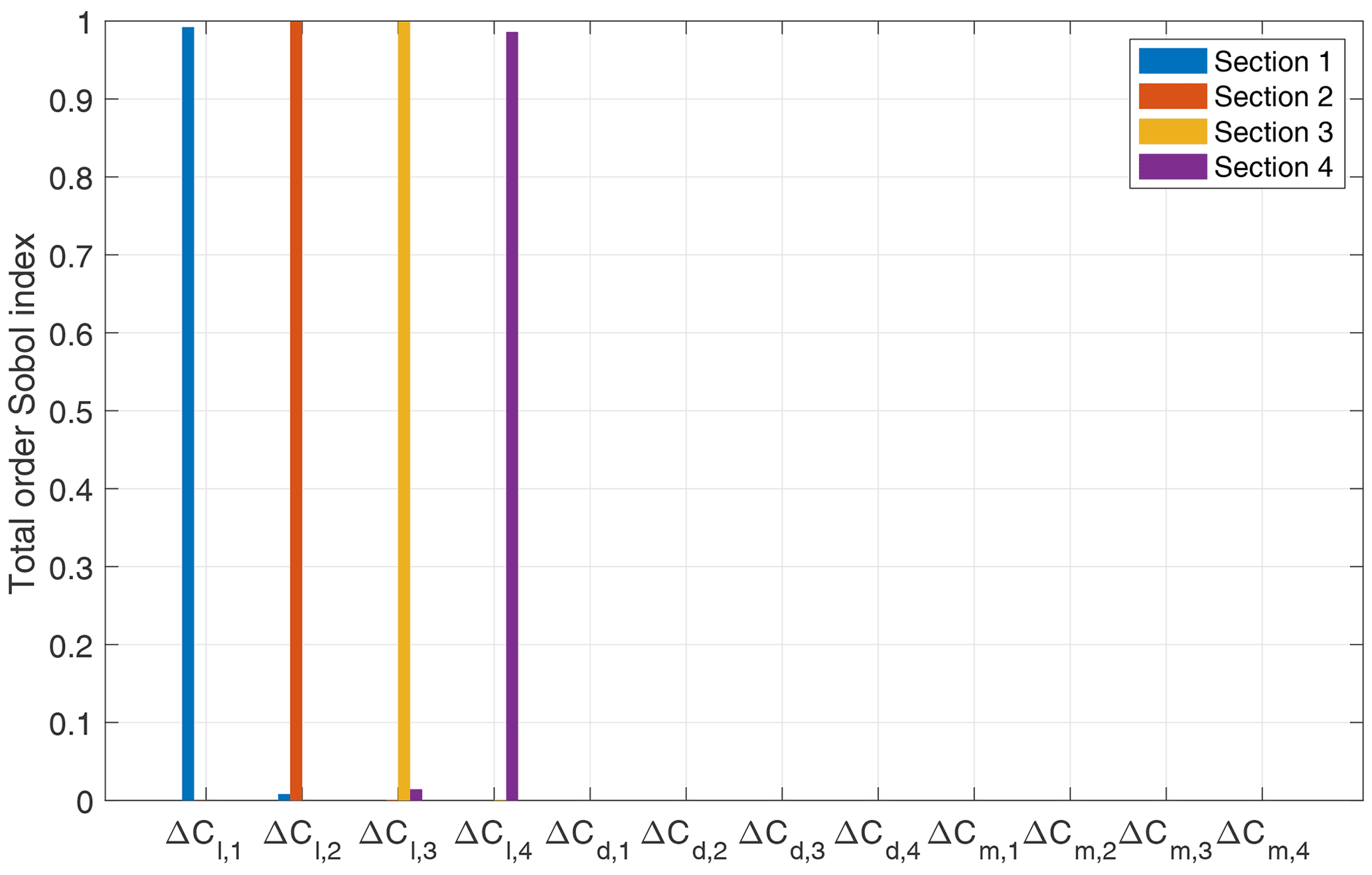
Figure 6 Sensitivity of sectional normal force with respect to perturbations in airfoil polars with adapted thickness.

5.1.2 Calibration

Following the sensitivity analysis, Bayesian calibration was performed for eight parameters, namely the four model parameters ΔC_l, 1–ΔC_l, 4 and the four discrepancy parameters θ_E, 1–θ_E, 4, using the normal force measurements obtained from the DANAERO MW experiment. The surrogate model constructed in Sect. 5.1.1 is retrained, without the drag and moment coefficients as uncertain parameters, again using N=32 runs of the Aero-Module. Since the sampling method is random (LHS), the surrogate model used for the calibration can in principle be somewhat different from the one used for the sensitivity analysis. In practice the surrogate model for calibration will be even more accurate, since it involves fewer parameters.

In the Bayesian analysis, the prior on the model parameters is taken the same as in Eq. (24). The prior on the discrepancy parameters is taken as a uniform distribution:

$$\begin{array}{}\text{(26)}& {\mathit{\theta }}_{E,i}\sim \mathcal{U}(\mathrm{0},{\mathit{\sigma }}_E^{\mathrm{2}}),i=\mathrm{1},\mathrm{\dots },\mathrm{4}.\end{array}$$

Note that θ_E (N² m⁻²) and ${\mathit{\sigma }}_E^{\mathrm{2}}$ model the variance between model and data and are therefore positive quantities. We take ${\mathit{\sigma }}_E^{\mathrm{2}}=\mathrm{5}\times {\mathrm{10}}^{\mathrm{4}}$ (so that σ_E≈223 N m⁻¹), which we determined by considering the standard deviation in the measurement data (around 100 N m⁻¹) and doubling this value to get a sufficiently broad prior. One could argue that this error should depend on the radial position along the blade, but this was not assumed in our prior specification. Instead, we did not want to introduce too much (possibly wrong or biased) a priori knowledge about the radial dependence but let the calibration process “do the job”.

The PCE-based surrogate model for the quantity of interest, Q^PC(θ_M), is used in place of the Aero-Module throughout the analyses. The AIES algorithm with 10² parallel chains and 10³ steps is deployed (in total 10⁵ MCMC iterations and concomitant surrogate model evaluations). Convergence is assessed based on the Gelman–Rubin diagnostic (Wagner et al., 2022) and visual inspection of the MCMC trace plots (see Fig. B4 in the Appendix), and a burn-in of 50 % is used. With the full Aero-Module, this would take several weeks to compute on a desktop computer. By using the surrogate model instead, this is reduced to less than an hour.

As discussed in Sect. 3.3.1, the number of measurements is varied to illustrate the effect on the posterior distribution of the parameters. As an example, Fig. 7a illustrates how the prior on ΔC_l, 1 (truncated normal) becomes more and more dominated by the data when the number of measurement points increases. The marginal posteriors for the other parameters show similar behavior. If additional data points were to be included, the posterior would become even stronger peaked (almost independent of the prior distribution).

Figure 7 Calibration results for the lift coefficient at the first radial section. (a) Posterior of ΔC_l, 1 with increasing number of measurements. (b) The calibrated C_l, 1 polar evaluated at the MAP of the posterior (obtained with 200 measurements), compared to the uncalibrated polar.

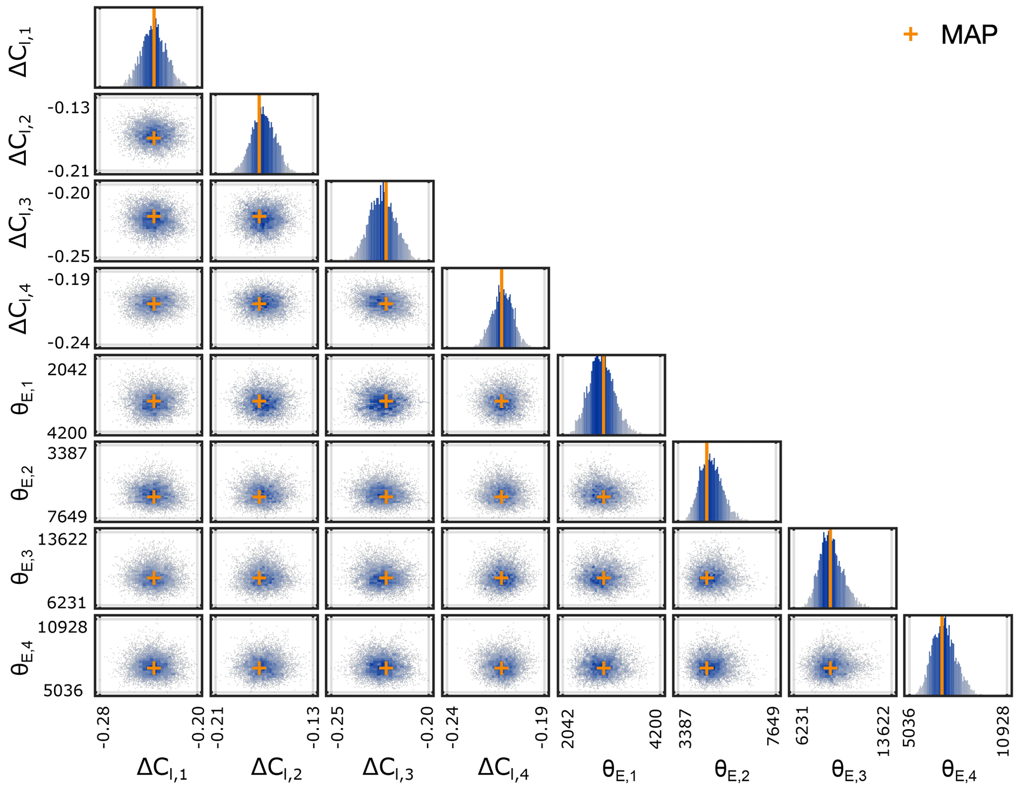
Figure 8 Samples of the posterior distribution of model parameters θ_M = ($\mathrm{\Delta }{C}_{\mathrm{l},\mathrm{1}}\mathrm{\dots }\mathrm{\Delta }{C}_{\mathrm{l},\mathrm{4}}$) and discrepancy parameters θ_E = (${\mathit{\theta }}_{E,\mathrm{1}}\mathrm{\dots }{\mathit{\theta }}_{E,\mathrm{4}}$) for the DANAERO test case with 200 measurements. The orange crosses correspond to the MAP estimates.

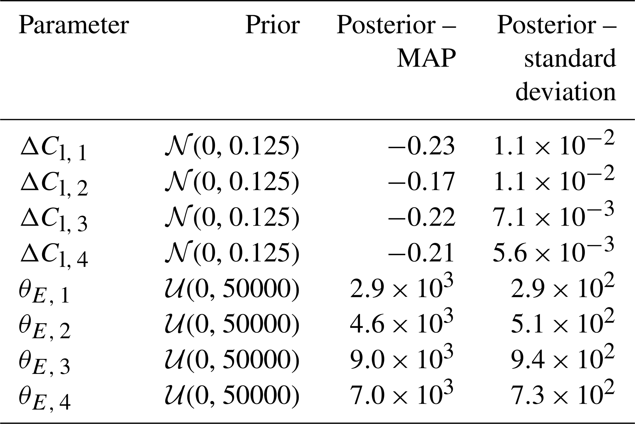
Table 2 Summary of prior and posterior distribution for DANAERO calibration with 200 measurements. ΔC_l is dimensionless, and θ_E has dimensions N² m⁻².

In what follows, we will focus on the case where 200 measurement points are used for the calibration. Figure 8 shows the resulting samples of the posterior distribution for all parameters. The ellipsoidal form of the two-dimensional scatterplots indicates that the different parameters are uncorrelated to good approximation. This is consistent with the outcome of the sensitivity analysis, which showed that each sectional lift force was basically only depending on the force coefficient at the very same section and not depending on the lift coefficient at other sections. Note that if the original thickness distribution were to be used (see Appendix B2), a strong correlation between the lift coefficients at Sects. 3 and 4 would show up.

A summary of the posterior marginals displayed in Fig. 8 is compiled in Table 2 in terms of the MAP and the standard deviation. Based on the MAP values, an example of a calibrated C_l polar, compared with the reference C_l polar, is shown in Fig. 7b. The MAP values of the lift coefficients all lie around −0.2, meaning that the original lift coefficients need to be corrected by about 20 % in order to match the experimental results (we will comment on this relatively large change in the next paragraph). Table 2 also lists the standard deviation associated with the ΔC_l parameters, which is in all cases small, confirming the observation of Fig. 7a that the posterior is sharply peaked when sufficient measurement points are included.

Given the samples of the posterior distribution, the posterior predictive distribution is computed following Eq. (23) and plotted along with the measurement data, the uncalibrated model results, and the model evaluated at the MAP in Fig. 9. Clearly, the calibrated Aero-Module (MAP) is overlapping with the mean of the experimental data. Furthermore, the posterior predictive (which expresses the probability of observing new data given the calibrated lift polars) centers nicely around the MAP and encapsulates the experimental data well. The results of the uncalibrated Aero-Module at the third and fourth radial section are very unlikely given the calibrated lift polars.

We note that in order to obtain the posterior predictive of other possible quantities of interest not considered in this work (such as the power output or the blade bending moment), one would preferably add these quantities to the model output list before the surrogate model is being trained, so that the posterior predictive can be efficiently evaluated without requiring full model runs. Alternatively, one could use the full Aero-Module with the calibrated parameters and use these to determine the posterior predictive for the power, but that would be computationally very expensive.

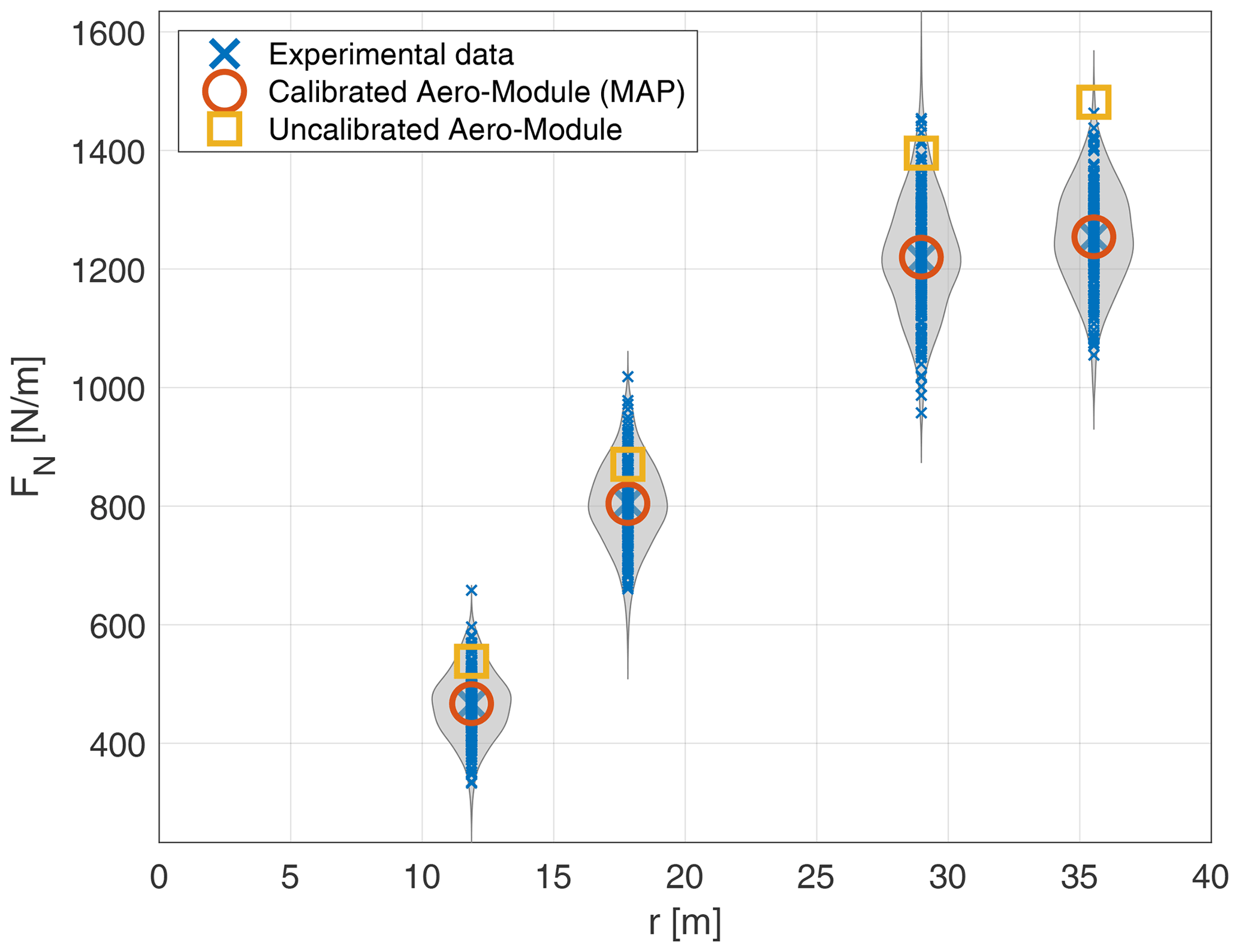
Figure 9 Comparison of uncalibrated and calibrated Aero-Module predictions of sectional normal forces with the DANAERO measurements. The grey shaded areas indicate the posterior predictive distributions. The large blue crosses indicate the mean of the measurement data (at each section), and the small crosses indicate the 200 measurements (at each section). The Aero-Module predictions are obtained from the surrogate model and are essentially indistinguishable from the full Aero-Module results, which have therefore been omitted for the sake of clarity.

It is important to note that using the obtained lift polars and hyperparameters in a predictive setting for a different set of operating conditions will require careful consideration. Firstly, using a single operating condition for calibrating the lift polars, as is currently the case, makes their validity to other operating conditions limited. Secondly, the discrepancy between model and measurement data (consisting of both model and measurement errors), E in Eq. (18), has been fully accounted for by calibrating the lift coefficient. It is highly likely that E depends also on other factors, such as the simplifications (missing physics) present in BEM theory, the unsteadiness of the atmospheric conditions, and the uncertainty in the measurements. This is perhaps the reason why that relatively large changes (around 20 %) in the sectional lift coefficients are needed to achieve a match between the Aero-Module and the experimental data. Lastly, the values obtained for the hyperparameters θ_E, 1–θ_E, 4 are very much dependent on the aerodynamic model and the data used. These values currently include both the measurement noise and the model inadequacy, which are not expected to be the same for a different set of measurements, a different operating condition, or a different aerodynamic model.

5.2 Yaw model calibration with New MEXICO data

In the previous section we showed as a proof of concept how the combination of surrogate modeling, sensitivity analysis, and Bayesian inference can be used to calibrate parameters of the Aero-Module. The test case was relatively simple in the sense that only a single operating condition was used, and because the relation between lift coefficient and normal force (Eq. 25) is linear, the sensitivity analysis and calibration results were quite straightforward. In this section we move to a more advanced test case, in which the parameters of a yaw model are calibrated based on normal force measurements.

5.2.1 Sensitivity analysis

As mentioned in Sect. 2.2, experiments and corresponding simulations were carried out for three different operating conditions; the values are shown in Table 1. The parameters to be calibrated are the yaw model parameters given by Eq. (7) and repeated here for convenience:

$$\begin{array}{}\text{(27)}& {\mathit{\theta }}_{\mathrm{M}}=({\text{AM}}_{\mathrm{11}},{\text{AM}}_{\mathrm{12}},{\text{AM}}_{\mathrm{13}},{\text{AM}}_{\mathrm{14}},{\text{AM}}_{\mathrm{15}}).\end{array}$$

The nominal (uncalibrated) values for these parameters are listed in Table C1 in Appendix C. A normal distribution is assumed for each amplitude coefficient, based on consultation with the developer of the yaw model (Schepers, 2012):

$$\begin{array}{}\text{(28)}& \text{AM}\sim \mathcal{N}(\mathit{\mu },\mathit{\sigma }),\end{array}$$

where μ equals the nominal value provided in Table C1, and σ is taken equal to 0.1. This value is such that the spread in the experimental data can be captured by the Aero-Module (as will be needed for calibration) and also makes sure that the induced velocity is likely to remain positive.

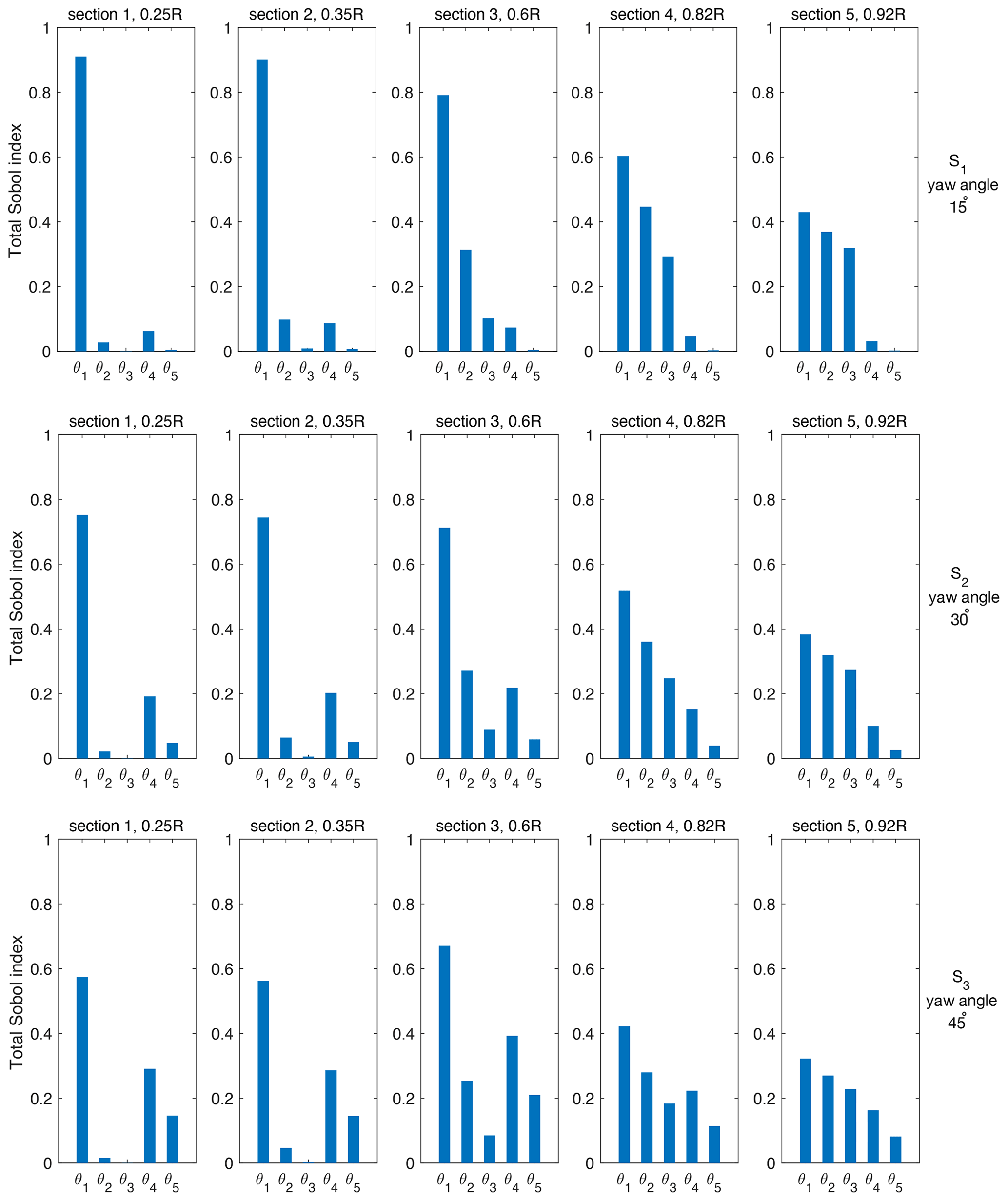
Figure 10 Sensitivity analysis for three different operating conditions: 𝒮₁ (top), 𝒮₂ (middle), and 𝒮₃ (bottom). Here ${\mathit{\theta }}_{\mathrm{M}}=({\mathit{\theta }}_{\mathrm{1}},{\mathit{\theta }}_{\mathrm{2}},{\mathit{\theta }}_{\mathrm{3}},{\mathit{\theta }}_{\mathrm{4}},{\mathit{\theta }}_{\mathrm{5}})=({\text{AM}}_{\mathrm{11}},{\text{AM}}_{\mathrm{12}},{\text{AM}}_{\mathrm{13}},{\text{AM}}_{\mathrm{14}},{\text{AM}}_{\mathrm{15}})$.

Similar to the previous case, a PCE is set up by drawing random samples from the parameter vector. In Appendix C the convergence of the LOO error is assessed, and it is shown that by taking N=256 samples (for each scenario) the LOO error is at most on the order of a few percent, which is sufficient to obtain accurate Sobol' indices (and to perform calibration). The total-order Sobol' indices S^T following Eq. (17) are computed for the five-dimensional parameter vector θ_M. In contrast to the DANAERO case (where the normal force at section i depended exclusively on the lift coefficient at section i), in this case the normal force at a certain section depends on the value of all model parameters, so that many more simulations are required to obtain an accurate surrogate model.

The resulting plots for the total Sobol' indices are shown in Fig. 10 for all three operating conditions. It is clear that parameter AM₁₁ is especially important at the inner part of the blade, whereas parameters AM₁₂ and AM₁₃ become increasingly important for the outboard sections. AM₁₄ and AM₁₅ have little dependency on r but instead increase in importance when the yaw angle is increased. This behavior is consistent with expression (C1). Overall, it can be concluded that all parameters are significantly influencing the normal force behavior (under the assumed distributions).

5.2.2 Calibration

The sensitivity analysis did not identify clear non-influential parameters, so all five yaw model parameters will be included in the calibration process. The experimental data for the calibration consist of the normal force measurements obtained from the New MEXICO experiment. However, the normal force measurements at Sect. 3 were not included in the calibration process, for the following reasons. Firstly, in Schepers et al. (2018) it was shown that the normal force amplitude measured at Sect. 3 (for case 2.1) appeared to be much lower than predicted by both BEM and computational fluid dynamics (CFD) codes. Secondly, it turned out that under the assumed range for the AM parameters, it was not possible to get amplitudes as small as reported in the measurement data (and this could not be fixed by increasing the range). Perhaps this could be fixed by including the other parameters of the yaw model, but it is also likely that the measurement data are off at this point. Therefore, the normal force at Sect. 3 has been removed from the surrogate model constructed in Sect. 5.2.1 for the purpose of calibration. The resulting PCE-based surrogate model for the quantity of interest, 𝒬^PC(θ_M), is based on 768 samples (256 for each scenario) and used in place of the Aero-Module throughout.

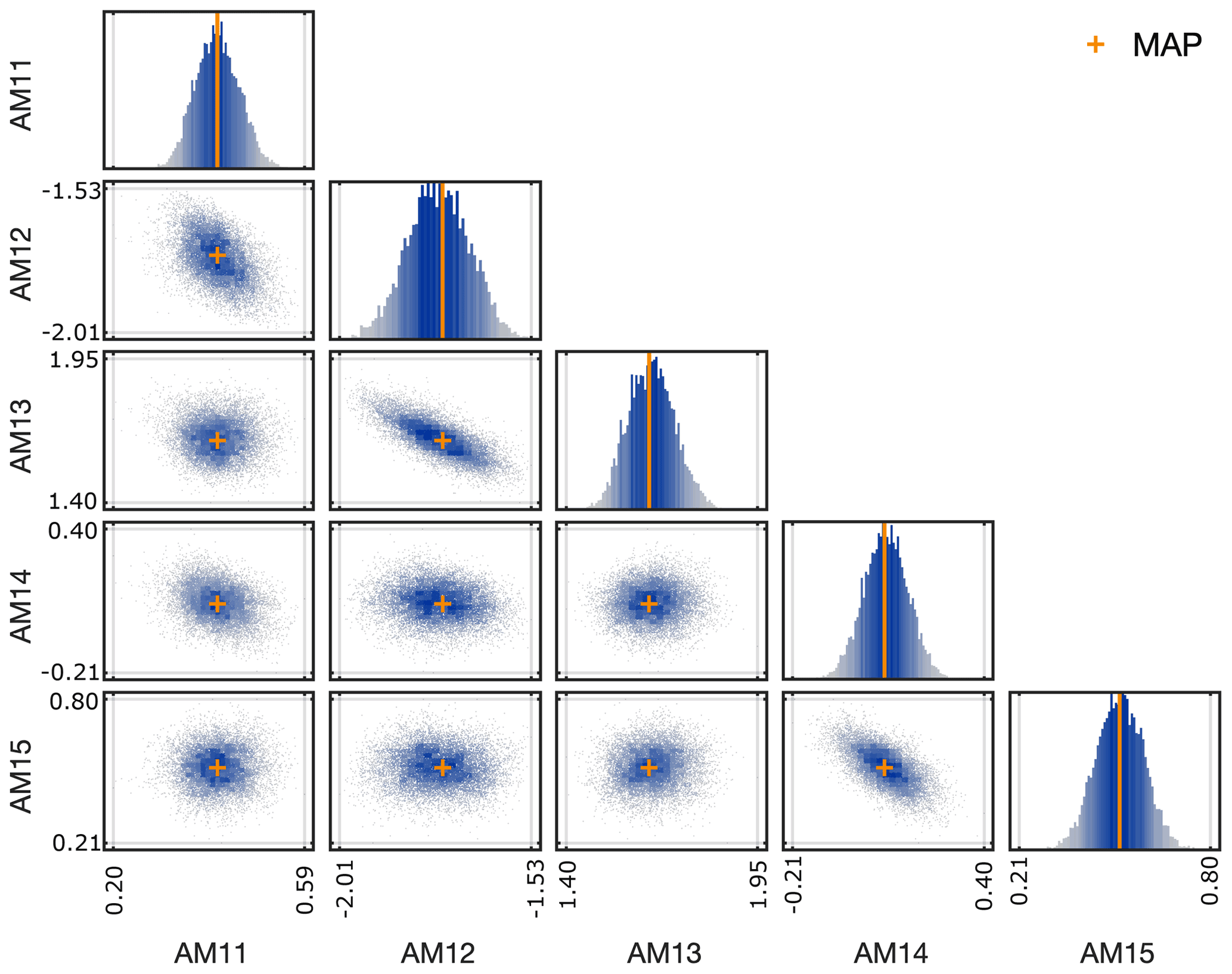
Figure 11 Samples of the posterior distribution of yaw model parameters for the New MEXICO test case. The orange crosses correspond to the MAP estimates.

The prior on the model parameters is taken the same as in Eq. (28). Given the limited number of measurement data, the discrepancy parameters are not calibrated in this test case but are chosen to be fixed (with the same value for each scenario and each radial section) at θ_E=σ², where σ is taken equal to 3 as a rough estimate based on the uncertainty bands reported in Schepers et al. (2018). Like in the previous test case, the AIES MCMC algorithm with 10³ steps and 10² parallel chains is deployed. The posterior samples and the marginal distributions are shown in Fig. 11, and corresponding statistics are given in Table 3 (for MCMC trace plot examples, we refer to Fig. C2 in Appendix C). One can observe that the posterior distributions are still Gaussian-like, but with a shifted mean and a smaller standard deviation than the prior distribution. The largest shift (in absolute sense) is incurred for parameters AM₁₄ and AM₁₅; the smallest shift happens for AM₁₃, which is hardly changed when compared to the prior. In contrast to the DANAERO test case, where the posterior was very much dominated by the data, the posterior for the New MEXICO case is still close to the prior, because fewer data points are used. The posterior samples indicate a clear correlation between parameters AM₁₂ and AM₁₃ and between AM₁₄ and AM₁₅. This result is consistent with the yaw model expression (Eq. C1), since AM₁₂ and AM₁₃ both relate to the relative radius, whereas AM₁₄ and AM₁₅ both relate to the yaw angle.

The normal force amplitudes that are obtained with the calibrated model parameters (based on the MAP) are shown for all operating conditions in Fig. 12, together with the measurement data and the uncalibrated model output. Overall, we observe that the calibration of the parameters has led to much improved model predictions. This is especially evident for the outboard sections for operating conditions 𝒮₂ and 𝒮₃. For other scenarios and/or radial sections also an improvement is generally observed, except for a few points, where the match is slightly worse (e.g., 𝒮₂, Sect. 2). Since the likelihood function in Bayes (Eq. 21 with covariance matrix chosen as Σ=σ²I) weighs the discrepancy in the different model outputs equally, it is not surprising that at some points the discrepancy can increase slightly, while at other points it is significantly reduced: on average the model fits the data much better.

Table 3 Summary of prior and posterior distribution for New MEXICO yaw model calibration.

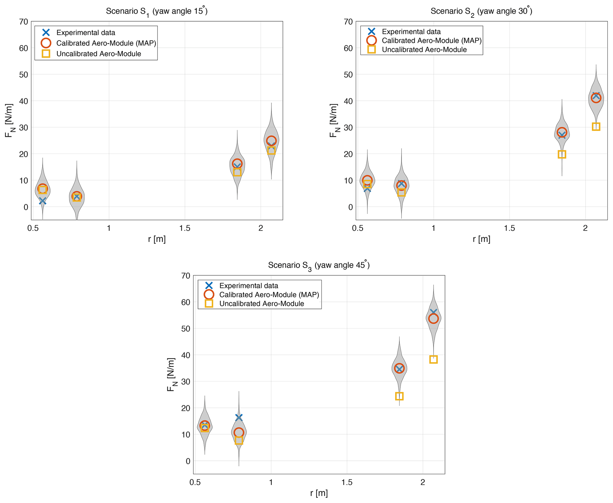
Figure 12 Comparison of uncalibrated and calibrated Aero-Module predictions with the New MEXICO measurements in terms of the normal force amplitude. The grey areas (violin plots) are constructed from 500 draws of the posterior predictive distribution. The Aero-Module predictions are obtained from the surrogate model and are essentially indistinguishable from the full Aero-Module results, which have therefore been omitted for the sake of clarity.

6 Conclusions

In this article we have proposed a computationally efficient framework to calibrate model parameters in aerodynamic wind turbine models. The three main ingredients that we use are (i) a (polynomial) surrogate model that approximates the wind turbine model, (ii) a sensitivity analysis to determine the most influential parameters, and (iii) Bayesian inference to calibrate parameters in a probabilistic setting. The Bayesian inference step, which is typically computationally very expensive to solve, is made computationally affordable through the use of the surrogate model. Evaluating 10⁵ MCMC iterations takes less than an hour with the surrogate model, whereas it would take weeks with the full Aero-Module model (when running on a desktop computer). The polynomial nature of the surrogate model furthermore allows quick evaluation of the Sobol' indices in the sensitivity analysis. The entire framework, known as UQ4Wind, is built around the UQLab software and tested on TNO's aerodynamic code Aero-Module.

Two realistic calibration studies have been performed with our proposed UQ4Wind framework in this paper. In the first test case, we have used part of the DANAERO experimental dataset to show how airfoil polars can be calibrated using normal force measurements. The sensitivity analysis clearly indicated that out of the lift, drag, and moment coefficients, the lift coefficient is most influential. After calibrating the lift coefficient values at the four radial sections, an excellent match with the experimental data was observed.

In the second test case, we have used part of the New MEXICO experimental dataset to calibrate five parameters of the yaw model that is used in the Aero-Module to estimate the induced velocity in yawed conditions. In order to handle the time dependence of both measurements and code output, we used a Fourier transform and considered the amplitude of the most dominant Fourier mode as the quantity of interest for the calibration. The calibrated model leads to much improved model predictions, especially regarding the normal force amplitude at the outboard sections of the blade under significant yaw misalignment.

In both cases, the result of the Bayesian approach consists of distributions of the calibrated model parameters (the posterior distribution). The posterior distribution allows us to make predictions under uncertainty, for example by computing the posterior predictive distribution, from which probabilistic statements can be deduced. At the same time, existing knowledge on the model parameters (e.g., expert knowledge) can be included via the prior distribution, and any relation (not necessarily Gaussian) between model and measurement data can be specified by choosing a likelihood function. These aspects form the true strength of the Bayesian approach. However, it should be realized that in the practical setting of calibrating an aerodynamic wind turbine model, it is not always clear how representative choices for the prior distribution or the likelihood are to be made. For the cases investigated in this paper, we have relied on expert knowledge and inspection of the measurement data. We acknowledge that this process should be carefully performed when considering different experimental datasets and/or model parameters. Similarly, the choice of distribution used in the sensitivity analysis (and in particular the corresponding variance) can determine to a large extent the Sobol' indices and has to be performed with care.

Another aspect that requires careful attention is the selection of proper datasets. Initially, the plan was to use more datasets from both DANAERO and New MEXICO in the calibration runs, but it turned out that many were not directly useful, for example because of non-constant operating conditions (DANAERO) or because the normal forces obtained from pressure distributions were not considered accurate enough in yawed conditions (New MEXICO). As an alternative, it is also possible to use models with a higher physical fidelity (e.g., free vortex wake models, which perform well in yawed conditions) to generate data for the calibration.

A last aspect for future consideration is that of the steady nature of the DANAERO test case, for which the airfoil polars could be calibrated without taking into account the effect of the dynamic stall model. In more realistic settings (e.g., turbulent inflow), one would have to calibrate both the airfoil polars and the dynamic stall model simultaneously. In the current case, time-dependent data were not available for further cross-validation, and the accuracy of the calibrated polars in dynamic flow conditions remains uncertain. We note that if such data were to be available, one should realize that the simultaneous calibration of both dynamic stall model parameters and airfoil polars would constitute a high-dimensional problem that might be computationally very expensive. Our approach, in which such effects are separated by using a time-dependent and a time-independent case, is effectively a way to reduce the high dimensionality of such a calibration problem.

Overall, we believe that the combination of surrogate modeling, sensitivity analysis, and Bayesian inference provides a powerful approach towards model calibration. Calibrated models with a quantified level of uncertainty have many applications in the wind energy industry beyond the aerodynamic models considered in this study, such as calibrating a dynamic wind farm control model (this is part of our ongoing work). Another topic within wind energy that could benefit from the UQ4WIND framework could be the calibration of low-order acoustic models using empirical correction factors for wind turbine noise estimation. Furthermore, calibration of engineering wake models, which typically contain several uncertain model parameters (such as wake expansion coefficients), would benefit from calibration using high-fidelity models such as CFD results.

Appendix A: Surrogate model details and UQLab settings

The surrogate model is built using LARS. The sampling scheme is Latin hypercube sampling (LHS) in all cases. Adaptive, sparse LARS is used, with possible polynomial degrees from 1 to 4 and truncation parameter 0.75 for DANAERO, as well as polynomial degrees from 1 to 10 and a truncation parameter range from 0.5 to 1.5 for New MEXICO.

For the sensitivity analysis, the main UQLab commands are

• uq_createInput (definition of model parameters),

• uq_createModel (once for definition of model and quantities of interest and once for setting up the PCE surrogate model), and

• uq_createAnalysis (determining Sobol' indices based on surrogate model).

For the Bayesian calibration, the same sequence of commands is used, with the difference that the uq_createAnalysis command then takes as input the options for the Bayesian calibration (prior, likelihood, experimental data, MCMC settings).

Appendix B: Details of lift polar calibration

B1 LOO convergence

The surrogate model should be accurately approximating the full Aero-Module in order to use it for sensitivity analysis and Bayesian inference. Figure B1a shows that the LOO error of the normal force at each airfoil section rapidly converges upon increasing the number of samples. The convergence of the LOO also becomes more regular when adapting the thickness distribution as will be described in the next Sect. B2, which can be observed in Fig. B1b. This is because the surrogate model at a certain section becomes almost independent of the parameters (lift coefficients) at other sections, making it easier to train. Note that the reported data points are obtained by averaging over five simulation runs (so for N=16 we perform 5×16 simulations) in order to smooth out the randomness introduced by the LHS sampling method. For the results in Sect. 5.1 we use the surrogate model with N=32.

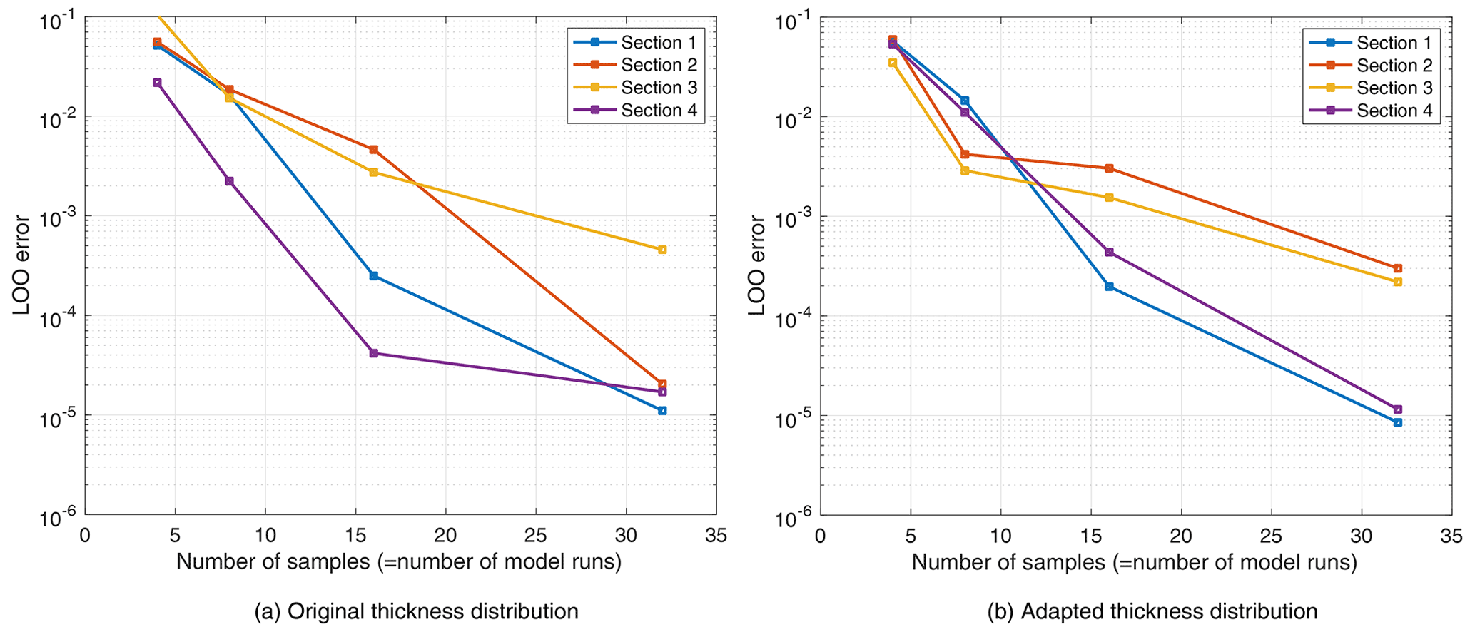
Figure B1 Convergence of LOO error as function of number of samples for DANAERO test case with 12 parameters. Each data point corresponds to the average over five runs. (a) Original thickness distribution. (b) Adapted thickness distribution.

B2 Thickness adaptation

When using the original input files to perform the DANAERO sensitivity study, it turned out that the normal force at Sect. 3 depended on the lift coefficient at both Sects. 3 and 4 (see Fig. B2). This peculiarity is caused by an inconsistency between the provided (planform) thickness distribution of the blade and the provided thickness of the four airfoil sections, as shown in Fig. B3. The lift coefficient at any radial position along the blade is determined by checking the local thickness in the planform graph and then interpolating the lift coefficient from nearby airfoil sections, based on the relative thickness. For example, at Sect. 3 (r=29 m), the planform thickness is around 0.189. This value lies in between the values of Sect. 3 ($t/c=\mathrm{0.197}$) and Sect. 4 ($t/c=\mathrm{0.187}$) but is much closer to Sect. 4 than Sect. 3. This explains the large effect of ΔC_l, 4 on the force at Sect. 3.

After consultation with the DANAERO experts, the thickness of the airfoil sections was changed to match the planform data (see Fig. B3). Figure 6 shows the results of the sensitivity analysis, indicating that with the adapted sectional thicknesses, we correctly obtain the expected dependency of the sectional normal force on the corresponding sectional lift coefficient. Thus, apart from identifying influential parameters, the sensitivity analysis step in our framework can also be used to correct inconsistencies in the model formulation.

B3 Calibration

Figure B4 shows two examples of the convergence of the MCMC chains for the parameter ΔC_l, 1 and hyperparameter θ_E, 1, where 200 data points were used for the calibration. The plot shows 100 chains that have been run for 1000 steps using the AIES algorithm. The trace plots for the other parameters show very similar behavior.

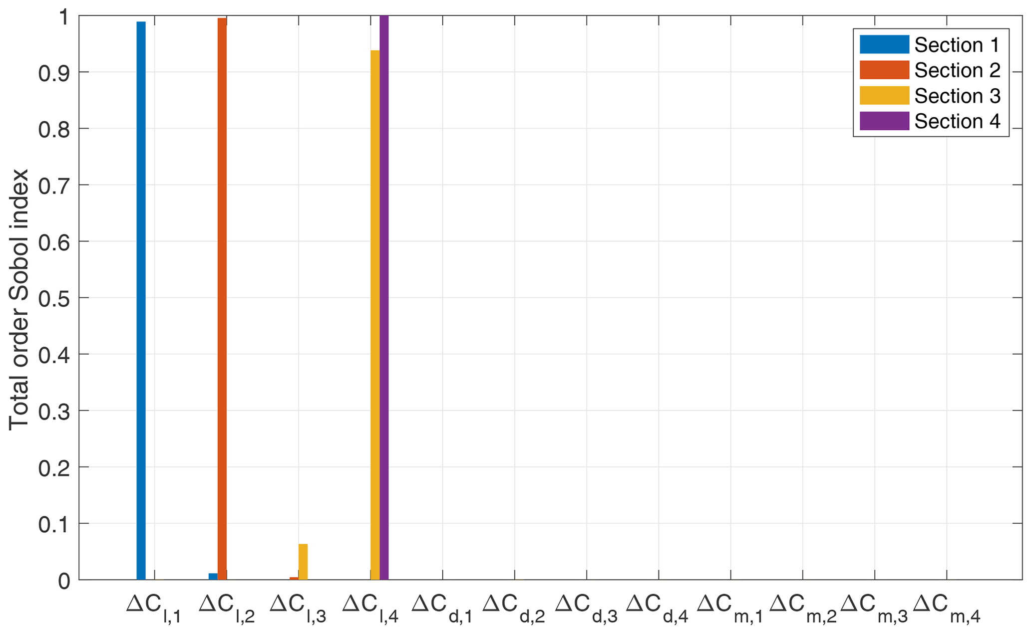
Figure B2 Sensitivity of sectional normal force with respect to perturbations in airfoil polars with original thickness.

Figure B3 Thickness distribution of DANAERO blade according to the planform data and the original and adapted airfoil sectional data. The discrepancy explains the observed sensitivity of the force at Sect. 3 towards the lift coefficient at Sect. 4.

Figure B4 Examples of MCMC chains and resulting posterior for model parameter ΔC_l, 1 and hyperparameter θ_E, 1, using 200 measurement points. For the results reported in Sect. 5.1, the first 50 % of the chains is discarded (so-called burn-in).

Appendix C: Details of yaw model calibration

The yaw model that is calibrated concerns an expression for the induced velocity (Schepers, 2012). The general form is

$$\begin{array}{}\text{(C1)}& \begin{array}{rl}& u_i(\stackrel{\mathrm{‾}}{r},\mathit{\beta },{\mathit{\varphi }}_r,{\mathit{\theta }}_{\mathrm{M}})=u_{i,\mathrm{0}}(\mathrm{1}-A_{\mathrm{1}}(\stackrel{\mathrm{‾}}{r},\mathit{\beta },{\mathit{\theta }}_{\mathrm{M}})\\ & \cos ({\mathit{\varphi }}_r-{\mathit{\psi }}_{\mathrm{1}}(\stackrel{\mathrm{‾}}{r},\mathit{\beta },{\mathit{\theta }}_{\mathrm{M}}\left)\right)-A_{\mathrm{2}}(\stackrel{\mathrm{‾}}{r},\mathit{\beta },{\mathit{\theta }}_{\mathrm{M}})\\ & \cos (\mathrm{2}{\mathit{\varphi }}_r-{\mathit{\psi }}_{\mathrm{2}}(\stackrel{\mathrm{‾}}{r},\mathit{\beta },{\mathit{\theta }}_{\mathrm{M}}\left)\right)).\end{array}\end{array}$$

Here $\stackrel{\mathrm{‾}}{r}$ is the relative radius ($\stackrel{\mathrm{‾}}{r}=r/R$), ϕ_r is the azimuth angle, and β is the yaw angle. In this study, we focus on ${\mathit{\theta }}_{\mathrm{M}}=\left({\mathrm{AM}}_{\mathrm{11}},\mathrm{\dots },{\mathrm{AM}}_{\mathrm{15}}\right)$, which appears in the expression for A₁:

$$\begin{array}{}\text{(C2)}& \begin{array}{rl}{A}_{\mathrm{1}}(\stackrel{\mathrm{‾}}{r},\mathit{\beta },{\mathit{\theta }}_{\mathrm{M}})& ={\mathrm{AM}}_{\mathrm{11}}+{\mathrm{AM}}_{\mathrm{12}}\stackrel{\mathrm{‾}}{r}+{\mathrm{AM}}_{\mathrm{13}}{\stackrel{\mathrm{‾}}{r}}^{\mathrm{2}}\\ & +{\mathrm{AM}}_{\mathrm{14}}\sin \left|\mathit{\beta }\right|+{\mathrm{AM}}_{\mathrm{15}}{\sin }^{\mathrm{2}}\mathit{\beta }.\end{array}\end{array}$$

Note that each parameter is multiplied by a factor that is between 0 and 1, since $\mathrm{0}\le \stackrel{\mathrm{‾}}{r}\le \mathrm{1}$ and $\mathrm{0}\le \mathit{\beta }\le \mathrm{90}{}^{\circ }$.

The nominal values for the yaw model parameters are given in Table C1 and taken from (Schepers, 2012).

The convergence of the LOO error for the New MEXICO case, for all three operating conditions, is shown in Fig. C1. Examples of MCMC trace plots for two selected parameters (AM₁₁ and AM₁₄) are shown in Fig. C2. The trace plots for the other parameters are similar.

Table C1 Summary of nominal value for yaw model parameters: amplitude coefficients (dimensionless).

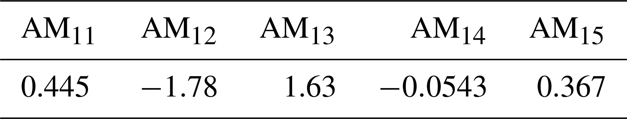
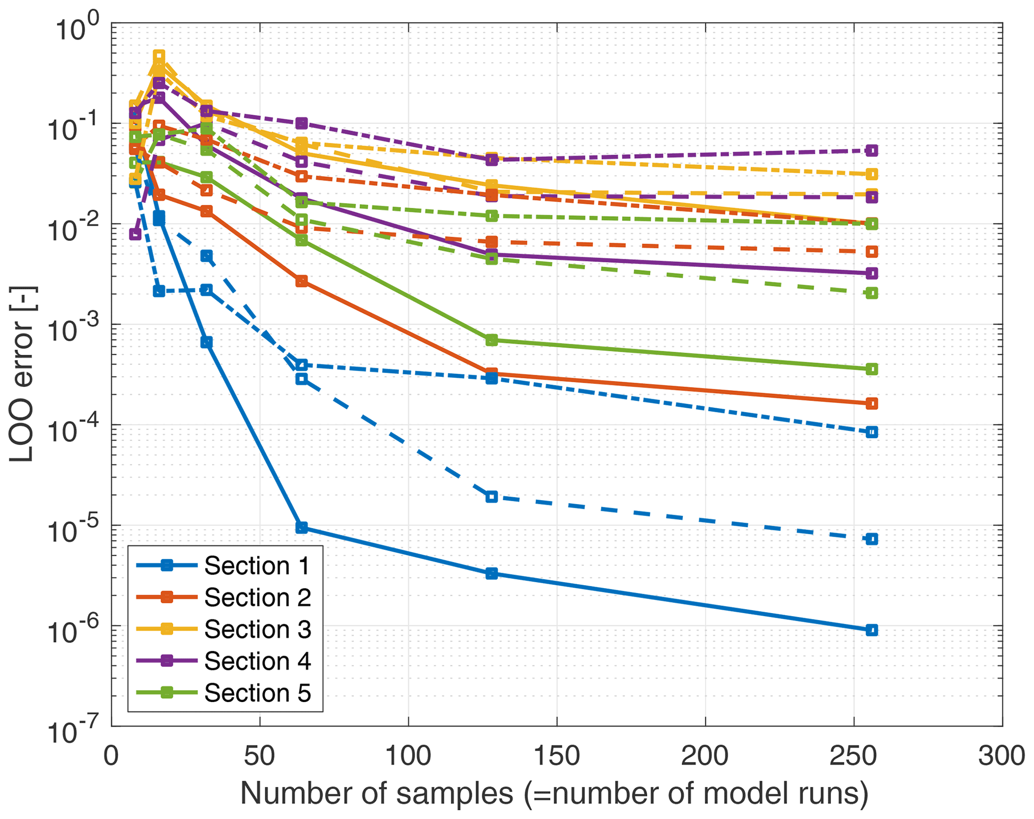
Figure C1 Surrogate model convergence for 𝒮₁ (dash–dot), 𝒮₂ (dashed), and 𝒮₃ (solid). Each data point corresponds to the average over five runs.

Figure C2 Examples of MCMC chains and resulting posterior for parameters AM₁₁ and AM₁₄. For the results reported in Sect. 5.2, the first 50 % of the chains is discarded (so-called burn-in).