Turbulence statistics from three different nacelle lidars

Atmospheric turbulence can be characterized by the Reynolds stress tensor, which consists of the second-order moments of the wind field components. Most of the commercial nacelle lidars cannot estimate all components of the Reynolds stress tensor due to their limited number of beams; most can estimate the along-wind velocity variance relatively well. Other components are however also important to understand the behavior of, e.g., the vertical wind profile and meandering of wakes. The SpinnerLidar, a research lidar with multiple beams and a very high sampling frequency, was deployed together with two commercial lidars in a forward-looking mode on the nacelle of a Vestas V52 turbine to scan the inflow. Here, we compare the lidar-derived turbulence estimates with those from a sonic anemometer using both numerical simulations and measurements from a nearby mast. We show that from these lidars, the SpinnerLidar is the only one able to retrieve all Reynolds stress components. For the two- and four-beam lidars, we study different methods to compute the along-wind velocity variance. By using the SpinnerLidar's Doppler spectra of the radial velocity, we can partly compensate for the lidar's probe volume averaging effect and thus reduce the systematic error of turbulence estimates. We find that the variances of the radial velocities estimated from the maximum of the Doppler spectrum are less affected by the lidar probe volume compared to those estimated from the median or the centroid of the Doppler spectrum.

1 Introduction

Understanding and measuring atmospheric turbulence are essential for the effective use of wind energy, to assess wind turbine site conditions, and for the assessment of the structural integrity of wind turbines. Traditionally, in situ anemometers installed on meteorological (met) masts are used to measure turbulence. However, with the increasing size of modern wind turbines, installing and operating a met mast that reaches the top of the rotor disk are becoming more and more expensive and infeasible. Nacelle lidars are compact and portable. They yaw with the wind turbine and scan over an area comparable to the rotor plane.

The Reynolds stress tensor is one of the most important turbulence statistics used in the wind energy industry. It consists of the second-order moments (variances and covariances) of the wind field components. One of the Reynolds stress components, the along-wind velocity variance, is used in the definition of turbulence intensity (IEC, 2019) and applied in different aspects of wind energy. Other components are also essential in wind energy and boundary-layer meteorology. For example, the vertical wind shear is connected to the friction velocity (Wyngaard, 2010), which can be computed using the momentum fluxes (two covariances); the momentum fluxes can also be used to crudely estimate the height of the boundary layer (Stull, 1988). The turbulence kinetic energy, expressed as half the sum of the three velocity components' variances, is a key parameter for investigating the turbulence structure in, e.g., wind turbine wakes (Kumer et al., 2016).

The main objective of this study is to investigate the benefit of using multiple-beam nacelle lidars for measuring inflow turbulence. Most commercial nacelle lidars are not able to estimate all components of the Reynolds stress tensor due to the limited number of beams and the scanning configuration. The SpinnerLidar is a research continuous-wave (CW) Doppler nacelle lidar. It scans at 400 positions at a high sampling frequency, which enables characterizing the inflow in detail. We evaluate and compare the turbulence characterization performance of a two- and a four-beam commercial lidar, and the SpinnerLidar through both numerical simulations and measurements inter-comparisons with in situ anemometers. For the latter, we deployed the three lidars in a forward-looking mode on the nacelle of a V52 wind turbine. Measurements from sonic anemometers on a met mast are used as reference for evaluation of the lidar-derived turbulence characteristics.

Assuming statistical homogeneity, we estimate the Reynolds stress components by fitting lidar radial velocity variances from the beams over the scanning pattern using a least-squares-based method. To determine the six components of the Reynolds stress tensor, we require at least six radial velocity variances measured in different beam orientations in analogy to the method by Eberhard et al. (1989). Here, we discuss the limitations of using different methods and assumptions to estimate the along-wind velocity variance with fewer than six radial velocity variances. We focus on this variance because it is a key parameter for load validation (Dimitrov et al., 2019; Conti et al., 2021), power performance assessment (Wagner et al., 2014, 2015; Borracino et al., 2017) and wind turbine control (Schlipf et al., 2014, 2020).

Measurements of turbulence by lidars are affected by spatial average filtering effects caused by the lidar probe volume and cross-contamination effects from combining line-of-sight velocities at different locations assuming instantaneous homogeneity and not only statistical homogeneity (Sathe and Mann, 2013; Kelberlau and Mann, 2020). Both effects contribute to the systematic error of turbulence estimation using lidars. As a consequence of the first effect, a lidar estimates turbulence essentially through a low-pass filter and cannot detect high-frequency variations, which yields the so-called “filtered variances”. Held and Mann (2018) showed that different methods of deriving the radial velocity from the lidar Doppler spectrum influence the degree of the turbulence attenuation. We explore the ability of these methods for turbulence estimation with the SpinnerLidar measurements. We also compensate for the probe volume filtering effect and compute “unfiltered variances” of the radial velocity using Doppler radial velocity spectra from the SpinnerLidar measurements. Peña et al. (2017) used Doppler radial velocity spectra and showed that the along-wind unfiltered variance from a conically scanning lidar agreed well with the one from a cup anemometer on a met mast. However, other lidar-derived estimates of velocity-component variances were largely biased due to the lidar scanning configuration.

This paper is organized as follows. Section 2 describes the turbulence spectral model, the maximum, median and centroid methods to derive the lidar radial velocities from the Doppler spectrum, the filtered and the unfiltered radial velocity variances, the least-squares method to compute the Reynolds stress tensor, and the numerical lidar simulations. Section 3 provides information on the measurement campaign and the employed nacelle lidars. Section 4 describes how we filter and post-process the high-frequency lidar radial velocities and the Doppler radial velocity spectra. Section 5 shows the inter-comparison of turbulence characteristics between three nacelle lidars and a mast-mounted sonic anemometer at turbine hub height. Discussions and conclusions are given in Sects. 6 and 7, respectively.

2 Methodology

2.1 Turbulence spectral model

Assuming Taylor's frozen turbulence hypothesis (Taylor, 1938), the wind field can be described by a vector field $\mathit{u}\left(\mathit{x}\right)=(u,v,w)=(u_{\mathrm{1}},u_{\mathrm{2}},u_{\mathrm{3}})$, where u is the horizontal along-wind component, v the horizontal lateral component, w the vertical component, and $\mathit{x}=(x,y,z)$ the position vector defined in a right-handed coordinate system. The mean value of the homogeneous velocity field is $\langle \mathit{u}\left(\mathit{x}\right)\rangle =(U,\mathrm{0},\mathrm{0})$, so the coordinate x is in the mean wind direction. The turbulence spectral properties of the three-dimensional homogeneous wind field are described by the spectral velocity tensor Φ_ij(k) (Kristensen et al., 1989):

$$\begin{array}{}\text{(1)}& {\mathrm{\Phi }}_{ij}\left(\mathit{k}\right)={\displaystyle \frac{\mathrm{1}}{(\mathrm{2}\mathit{\pi }{)}^{\mathrm{3}}}}\int R_{ij}\left(\mathit{x}\right)\text{exp}(-i\mathit{k}\cdot \mathit{x})\mathrm{d}\mathit{x},\end{array}$$

which is the Fourier transform of the covariance tensor $R_{ij}\left(\mathit{x}\right)\equiv \langle u_i^{\prime }\left(\mathit{x}\right)u_j^{\prime }(\mathit{x}+\mathit{r})\rangle$, where 〈 〉 denotes ensemble averaging, r is the separation vector, $u_i^{\prime }$ are the fluctuations around the mean and $\mathit{k}=(k_{\mathrm{1}},k_{\mathrm{2}},k_{\mathrm{3}})$ is the wave vector in the $(x,y,z)$ directions.

We assume that the spectral velocity tensor Φ_ij(k) can be described by the model of Mann (1994) (hereafter the Mann model), which, besides k, only contains three parameters (known as Mann parameters): $\mathit{\alpha }{\mathit{\epsilon }}^{\mathrm{2}/\mathrm{3}}$ is a product of the spectral Kolmogorov constant α and the turbulent energy dissipation rate ε to the two-thirds power, L is a length scale related to the size of the energy-containing eddies, and Γ is a parameter describing the anisotropy of the turbulence. From the spectral tensor, the one-point spectra of velocity fluctuations are calculated by

$$\begin{array}{}\text{(2)}& F_{ij}\left(k_{\mathrm{1}}\right)=\iint {\mathrm{\Phi }}_{ij}\left(\mathit{k}\right)\mathrm{d}{k}_{\mathrm{2}}\mathrm{d}{k}_{\mathrm{3}}.\end{array}$$

The wind velocity components have the three auto-spectra F₁₁ (=F_u), F₂₂, and F₃₃. The auto-spectra can be evaluated using Eq. (2). The variances of the velocity components are

$$\begin{array}{}\text{(3)}& {\mathit{\sigma }}_{u,v,w}^{\mathrm{2}}=\underset{-\mathrm{\infty }}{\overset{\mathrm{\infty }}{\int }}{F}_{u,v,w}\left(k_{\mathrm{1}}\right)\mathrm{d}{k}_{\mathrm{1}},\end{array}$$

and these, together with the covariances, are the components of the Reynolds stress tensor:

$$\begin{array}{}\text{(4)}& \mathit{R}=\left[\begin{array}{ccc}{\mathit{\sigma }}_u^{\mathrm{2}}& \langle u^{\prime }{v}^{\prime }\rangle & \langle u^{\prime }{w}^{\prime }\rangle \\ \langle v^{\prime }{u}^{\prime }\rangle & {\mathit{\sigma }}_v^{\mathrm{2}}& \langle v^{\prime }{w}^{\prime }\rangle \\ \langle w^{\prime }{u}^{\prime }\rangle & \langle w^{\prime }{v}^{\prime }\rangle & {\mathit{\sigma }}_w^{\mathrm{2}}\end{array}\right].\end{array}$$

2.2 Nacelle lidar

The unit vector n describing the beam orientation of a nacelle lidar can be expressed as (Peña et al., 2017)

$$\begin{array}{}\text{(5)}& \mathit{n}(\mathit{\varphi },\mathit{\theta })=(-\cos \mathit{\varphi },\cos \mathit{\theta }\sin \mathit{\varphi },\sin \mathit{\theta }\sin \mathit{\varphi }),\end{array}$$

where θ is the angle between the y axis and n projected onto the y–z plane and ϕ is the angle between the beam and the negative x axis (hereafter half-cone opening angle). As with any other Doppler lidar, nacelle lidars only measure the radial velocity (also known as the line-of-sight velocity) along the laser beam. Thus, the radial velocity can be expressed as (Mann et al., 2010)

$$\begin{array}{}\text{(6)}& v_{\mathrm{r}}(\mathit{\varphi },\mathit{\theta })=\underset{-\mathrm{\infty }}{\overset{\mathrm{\infty }}{\int }}\mathit{\phi }\left(s\right)\mathit{n}(\mathit{\varphi },\mathit{\theta })\cdot \mathit{u}\left[\mathit{n}\right(\mathit{\varphi },\mathit{\theta }\left)\right(f_d+s\left)\right]\mathrm{d}s,\end{array}$$

where φ is the lidar weighting function that considers the probe volume, s is the distance from the focus point along the beam and f_d is the focus distance. This equation assumes that v_r is determined from the Doppler spectrum by the centroid or center of gravity method. For the case of the investigated CW lidars, their weighting functions are assumed to be of the Lorentzian form (Sonnenschein and Horrigan, 1971):

$$\begin{array}{}\text{(7)}& \mathit{\phi }\left(s\right)={\displaystyle \frac{\mathrm{1}}{\mathit{\pi }}}{\displaystyle \frac{z_{\mathrm{R}}}{z_{\mathrm{R}}^{\mathrm{2}}+s^{\mathrm{2}}}},\end{array}$$

where z_R is the Rayleigh length that can be estimated as

$$\begin{array}{}\text{(8)}& z_{\mathrm{R}}={\displaystyle \frac{\mathit{\lambda }{f}_d^{\mathrm{2}}}{\mathit{\pi }{r}_{\mathrm{b}}^{\mathrm{2}}}},\end{array}$$

where λ is the laser wavelength and r_b the beam radius at the output lens.

If we assume that the lidars measure at a point, instead of over a probe volume, and that u, v and w do not change over the scanned area, the radial velocity in Eq. (6) can be estimated as the sum of the projection of the three-dimensional wind components on the beam pointing direction:

$$\begin{array}{}\text{(9)}& v_{\mathrm{r}}(\mathit{\varphi },\mathit{\theta })=-u\cos \mathit{\varphi }+v\cos \mathit{\theta }\sin \mathit{\varphi }+w\sin \mathit{\theta }\sin \mathit{\varphi }.\end{array}$$

The variance of the radial velocity ${\mathit{\sigma }}_{v_{\mathrm{r}}}^{\mathrm{2}}$ can be derived by taking the variance of Eq. (9) (Eberhard et al., 1989):

$$\begin{array}{ll}{\displaystyle }{\mathit{\sigma }}_{v_{\mathrm{r}},\text{unf}}^{\mathrm{2}}(\mathit{\varphi },\mathit{\theta })=& {\displaystyle }{\mathit{\sigma }}_u^{\mathrm{2}}{\cos }^{\mathrm{2}}\mathit{\varphi }+{\mathit{\sigma }}_v^{\mathrm{2}}{\cos }^{\mathrm{2}}\mathit{\theta }{\sin }^{\mathrm{2}}\mathit{\varphi }+{\mathit{\sigma }}_w^{\mathrm{2}}{\sin }^{\mathrm{2}}\mathit{\theta }{\sin }^{\mathrm{2}}\mathit{\varphi }\\ {\displaystyle }& {\displaystyle }-\mathrm{2}\langle u^{\prime }{v}^{\prime }\rangle \cos \mathit{\varphi }\cos \mathit{\theta }\sin \mathit{\varphi }\\ {\displaystyle }& {\displaystyle }-\mathrm{2}\langle u^{\prime }{w}^{\prime }\rangle \cos \mathit{\varphi }\sin \mathit{\theta }\sin \mathit{\varphi }\\ \text{(10)}& {\displaystyle }& {\displaystyle }+\mathrm{2}\langle v^{\prime }{w}^{\prime }\rangle {\sin }^{\mathrm{2}}\mathit{\varphi }\cos \mathit{\theta }\sin \mathit{\theta }.\end{array}$$

Equation (10) provides accurate velocity-component variance and covariance estimates if the radial velocity variance is unfiltered, i.e., if we are able to account for the lidar probe volume. In practice, if the Doppler radial velocity spectrum is available, we have means to estimate the unfiltered radial velocity variance. This will be described in Sect. 2.4.

2.3 Estimation of the radial velocity and the filtered radial velocity variance

Three methods are used here to determine the dominant frequency from the Doppler radial velocity spectrum to compute the radial velocity. The centroid method computes the characteristic frequency f in the Doppler radial velocity spectrum p(f) as

$$\begin{array}{}\text{(11)}& f_{\text{cen}}={\displaystyle \frac{\int fp\left(f\right)\mathrm{d}f}{\int p\left(f\right)\mathrm{d}f}}.\end{array}$$

The maximum method finds the frequency bin where the maximum peak in the Doppler spectrum occurs. The median method treats the Doppler spectrum as a probability distribution and finds the frequency bin that corresponds to the median value. These frequencies are then converted to radial velocity estimates according to the sampling frequency of the digitizer, the length of the fast Fourier transform, and the lidar's laser wavelength. Since none of these methods considers the whole Doppler radial velocity spectrum, turbulence statistics computed from these radial velocities are filtered. Therefore, we use the term-filtered radial velocity variance ${\mathit{\sigma }}_{v_{\mathrm{r}},\text{filt}}^{\mathrm{2}}$.

2.4 Estimation of the unfiltered radial velocity variance

Here, we use the Doppler radial velocity spectrum to estimate the unfiltered radial velocity variance ${\mathit{\sigma }}_{v_{\mathrm{r}},\text{unf}}^{\mathrm{2}}$ of the lidar beams. Since the investigated nacelle lidars measure at small opening angles over a relatively homogeneous inflow, the effect of the radial velocity gradient within the probe volume is negligible (see Mann et al., 2010, for a detailed discussion). Therefore, ${\mathit{\sigma }}_{v_{\mathrm{r}},\text{unf}}^{\mathrm{2}}$ can be estimated as the second central statistical moment of the ensemble-average Doppler spectrum of the radial velocity. The mean radial velocity can be estimated from the area-normalized mean Doppler spectrum p(v_r) as

$$\begin{array}{}\text{(12)}& {\mathit{\mu }}_{v_{\mathrm{r}}}=\underset{-\mathrm{\infty }}{\overset{\mathrm{\infty }}{\int }}{v}_{\mathrm{r}}p\left(v_{\mathrm{r}}\right)\mathrm{d}{v}_{\mathrm{r}},\end{array}$$

and its variance as

$$\begin{array}{}\text{(13)}& {\mathit{\sigma }}_{v_{\mathrm{r}}}^{\mathrm{2}}=\underset{-\mathrm{\infty }}{\overset{\mathrm{\infty }}{\int }}(v_{\mathrm{r}}-{\mathit{\mu }}_{v_{\mathrm{r}}}{)}^{\mathrm{2}}p(v_{\mathrm{r}})\mathrm{d}{v}_{\mathrm{r}}.\end{array}$$

Assuming all radial velocity contributions to the Doppler spectrum are due to turbulence, ${\mathit{\sigma }}_{v_{\mathrm{r}}}^{\mathrm{2}}$ in Eq. (13) provides an estimate of ${\mathit{\sigma }}_{v_{\mathrm{r}},\text{unf}}^{\mathrm{2}}$. This can be used to extract the velocity variances using Eq. (10), which gives the components of the Reynolds stress tensor.

2.5 Estimation of the mean wind velocity

Radial velocity measurements from different beam directions can be combined to reconstruct the mean wind. In the following sections, we show that different approaches are used for different lidars.

2.5.1 First approach

A least-squares formulation is used to find the mean wind vector $\mathit{U}=(U,V,W)$ over all beam positions. Here, we minimize the sum of squared differences between the beam-projected wind and the measured radial velocities:

$$\begin{array}{}\text{(14)}& {\mathrm{\Delta }}^{\mathrm{2}}=\int (\mathit{n}\cdot \mathit{U}-v_{\mathrm{r}}{)}^{\mathrm{2}}\mathrm{d}\mathit{\mu }.\end{array}$$

The integral ∫dμ could be an area-weighted average of the beam measurements. In practice, the integral could simply be the sum over all pairs of radial velocity v_r and the corresponding beam unit vectors n among the scanning area. The vector U that minimizes the integral must fulfill

$$\begin{array}{}\text{(15)}& {\displaystyle \frac{\partial {\mathrm{\Delta }}^{\mathrm{2}}}{\partial U_i}}=\mathrm{0}\Rightarrow \int (\mathit{n}\cdot \mathit{U}-v_{\mathrm{r}})n_i\mathrm{d}\mathit{\mu }=\mathrm{0},\text{for}i=\mathrm{1},\mathrm{2},\mathrm{3}.\end{array}$$

Expanding the integral and isolating U we get

$$\begin{array}{}\text{(16)}& U_i=(M^{-\mathrm{1}}{)}_{ij}\int v_{\mathrm{r}}{n}_i\mathrm{d}\mathit{\mu },\text{where}{M}_{ij}=\int n_i{n}_j\mathrm{d}\mathit{\mu }.\end{array}$$

This approach assumes wind homogeneity over the scanning area. To get the three mean wind components, we need at least three values of v_r measured in different orientations. This approach is used for deriving the mean wind vector from SpinnerLidar multi-beam measurements.

2.5.2 Second approach

Assuming that the inflow wind is horizontal, i.e., w=0 m s⁻¹, Eq. (9) can here be reduced to

$$\begin{array}{}\text{(17)}& v_{\mathrm{r}}(\mathit{\varphi },\mathit{\theta })=u\cos \mathit{\varphi }+v\sin \mathit{\varphi }\cos \mathit{\theta }.\end{array}$$

To compute the mean wind components, we need at least two radial velocities measurements and the corresponding beam positions (ϕ and θ) assuming that u and v are identical at the focus points of a pair of beams. Therefore, a two-beam nacelle lidar can compute u and v:

$$\begin{array}{ll}{\displaystyle }u& {\displaystyle }={\displaystyle \frac{v_{\text{r,left}}+v_{\text{r,right}}}{\mathrm{2}\cos \mathit{\varphi }}},\\ \text{(18)}& {\displaystyle }v& {\displaystyle }={\displaystyle \frac{v_{\text{r,right}}-v_{\text{r,left}}}{\mathrm{2}\sin \mathit{\varphi }}}.\end{array}$$

A similar approach can be used for a four-beam nacelle lidar. The two upper beams and two lower beams are used separately (Larvol, 2016) to estimate u and v at two different heights. Here, we average the estimates at the two heights to represent the mean inflow velocity.

2.5.3 Induction correction

Due to the presence of the wind turbine, the wind slows down as it approaches the rotor. We perform the correction of the slowdown in speed (also referred as the induction correction) to the estimates of lidars and the sonic anemometer using the method in Simley et al. (2016):

$$\begin{array}{}\text{(19)}& {\displaystyle \frac{U}{U_{\mathrm{\infty }}}}=\mathrm{1}-a\left(\mathrm{1}+{\displaystyle \frac{\mathrm{2}x}{D}}{\left(\mathrm{1}+{\left({\displaystyle \frac{\mathrm{2}x}{D}}\right)}^{\mathrm{2}}\right)}^{-\frac{\mathrm{1}}{\mathrm{2}}}\right),\end{array}$$

where U_∞ is the undisturbed free stream wind speed, x is the distance between the lidar scanning plane and the rotor, and a is the axial induction factor. The induction factor a is determined using the same procedure as the one in Held and Mann (2019) assuming the effect of the induction is constant over a 10 min period. A steady-state thrust curve of the V52 turbine and the 10 min mean wind speeds measured by the cup anemometer at 44 m are used to look up the thrust coefficient C_t. Then, we compute the induction factor using axial momentum theory, i.e., $C_{\mathrm{t}}=\mathrm{4}a(\mathrm{1}-a)$.

2.6 Estimation of the Reynolds stress tensor

We assume that the Reynolds stresses R_ij≡〈u_iu_j〉 are homogeneous over the rotor plane irrespective of the mean wind field. We apply a least-squares fit to the radial velocity variances and the corresponding beam unit vectors to estimate the Reynolds stresses:

$$\begin{array}{}\text{(20)}& {\mathrm{\Delta }}^{\mathrm{2}}=\int (\mathit{n}\cdot \mathit{R}\mathit{n}-{\mathit{\sigma }}_{v_{\mathrm{r}}}^{\mathrm{2}}{)}^{\mathrm{2}}\mathrm{d}\mathit{\mu }.\end{array}$$

The matrix R that minimizes the integral must fulfill

$$\begin{array}{}\text{(21)}& {\displaystyle \frac{\partial {\mathrm{\Delta }}^{\mathrm{2}}}{\partial R_{ij}}}=\mathrm{0}\Rightarrow \int (\mathit{n}\cdot \mathit{R}\mathit{n}-{\mathit{\sigma }}_{v_{\mathrm{r}}}^{\mathrm{2}})n_i{n}_j\mathrm{d}\mathit{\mu }=\mathrm{0}.\end{array}$$

This can be written as

$$\begin{array}{}\text{(22)}& R_{kl}\int n_k{n}_l{n}_i{n}_j\mathrm{d}\mathit{\mu }=\int {\mathit{\sigma }}_{v_{\mathrm{r}}}^{\mathrm{2}}{n}_i{n}_j\mathrm{d}\mathit{\mu }.\end{array}$$

The right side of Eq. (22) is written as a vector having the length of six using the six combinations of indices $(i,j)=(\mathrm{1},\mathrm{1}),(\mathrm{1},\mathrm{2}),(\mathrm{1},\mathrm{3}),(\mathrm{2},\mathrm{2}),(\mathrm{2},\mathrm{3}),(\mathrm{3},\mathrm{3})$ with $n_{\mathrm{1}}=-\cos \mathit{\varphi }$, n₂=cos θsin ϕ and n₃=sin θsin ϕ (as given in Eq. 5). Similarly, on the left side of Eq. (22), R_kl is rearranged to a length six vector, where ∫n_kn_ln_in_jdμ is a 6-by-6 matrix with both (k,l) and (i,j) going through the same combinations of indices:

$$\begin{array}{}\text{(23)}& \begin{array}{rl}& \left[\begin{array}{cccccc}\sum n_{\mathrm{1}}^{\mathrm{4}}& \sum n_{\mathrm{1}}^{\mathrm{2}}{n}_{\mathrm{2}}^{\mathrm{2}}& \sum n_{\mathrm{1}}^{\mathrm{2}}{n}_{\mathrm{3}}^{\mathrm{2}}& \sum \mathrm{2}{n}_{\mathrm{1}}^{\mathrm{3}}{n}_{\mathrm{2}}& \sum \mathrm{2}{n}_{\mathrm{1}}^{\mathrm{3}}{n}_{\mathrm{3}}& \sum \mathrm{2}{n}_{\mathrm{1}}^{\mathrm{2}}{n}_{\mathrm{2}}{n}_{\mathrm{3}}\\ \mathrm{\dots }& \sum n_{\mathrm{2}}^{\mathrm{4}}& \mathrm{\dots }& \mathrm{\dots }& \mathrm{\dots }& \mathrm{\dots }\\ \mathrm{\dots }& \mathrm{\dots }& \sum n_{\mathrm{3}}^{\mathrm{4}}& \mathrm{\dots }& \mathrm{\dots }& \mathrm{\dots }\\ \mathrm{\dots }& \mathrm{\dots }& \mathrm{\dots }& \sum \mathrm{2}{n}_{\mathrm{1}}^{\mathrm{2}}{n}_{\mathrm{2}}^{\mathrm{2}}& \mathrm{\dots }& \mathrm{\dots }\\ \mathrm{\dots }& \mathrm{\dots }& \mathrm{\dots }& \mathrm{\dots }& \sum \mathrm{2}{n}_{\mathrm{1}}^{\mathrm{2}}{n}_{\mathrm{3}}^{\mathrm{2}}& \mathrm{\dots }\\ \mathrm{\dots }& \mathrm{\dots }& \mathrm{\dots }& \mathrm{\dots }& \mathrm{\dots }& \sum \mathrm{2}{n}_{\mathrm{2}}^{\mathrm{2}}{n}_{\mathrm{3}}^{\mathrm{2}}\end{array}\right]\\ & \times \left[\begin{array}{c}{R}_{uu}\\ R_{vv}\\ R_{ww}\\ R_{uv}\\ R_{uw}\\ R_{vw}\end{array}\right]=\left[\begin{array}{c}\sum {\mathit{\sigma }}_{v_{\mathrm{r}}}^{\mathrm{2}}{n}_{\mathrm{1}}^{\mathrm{2}}\\ \sum {\mathit{\sigma }}_{v_{\mathrm{r}}}^{\mathrm{2}}{n}_{\mathrm{2}}^{\mathrm{2}}\\ \sum {\mathit{\sigma }}_{v_{\mathrm{r}}}^{\mathrm{2}}{n}_{\mathrm{3}}^{\mathrm{2}}\\ \sum {\mathit{\sigma }}_{v_{\mathrm{r}}}^{\mathrm{2}}{n}_{\mathrm{1}}{n}_{\mathrm{2}}\\ \sum {\mathit{\sigma }}_{v_{\mathrm{r}}}^{\mathrm{2}}{n}_{\mathrm{1}}{n}_{\mathrm{3}}\\ \sum {\mathit{\sigma }}_{v_{\mathrm{r}}}^{\mathrm{2}}{n}_{\mathrm{2}}{n}_{\mathrm{3}}\end{array}\right].\end{array}\end{array}$$

To compute the six Reynolds stresses, we need at least six radial velocity variances from different beam directions to ensure that the large matrix in Eq. (23) is not degenerate (i.e., its determinant is not zero) (Sathe et al., 2015). If fewer than six variances of the radial velocity are available, we have fewer knowns than unknowns. If the nacelle lidar beams have only one opening angle ϕ, the equations will be linearly dependent, and so the determinant will be zero and Eq. (23) will have infinite solutions. In those cases, only ${\mathit{\sigma }}_u^{\mathrm{2}}$ can be well determined, and the stresses involving the lateral component will be more noisy (Peña et al., 2019). In this study, we use all radial velocity variances from the SpinnerLidar to calculate the six Reynolds stresses.

2.7 Numerical simulations

We generate three-dimensional random turbulence fields using the Mann model (Mann, 1998) with typical values of the model parameters: $\mathit{\alpha }{\mathit{\epsilon }}^{\mathrm{2}/\mathrm{3}}=\mathrm{0.05}$ ${\mathrm{m}}^{\mathrm{4}/\mathrm{3}}{\mathrm{s}}^{-\mathrm{1}}$, L=61 m and Γ=3.2. We furthermore assume Taylor's frozen turbulence hypothesis:

$$\begin{array}{}\text{(24)}& \mathit{u}(x,y,z,t=\mathrm{0})=\mathit{u}(x+Ut,y,z,t),\end{array}$$

so the wind field at any given time can be obtained by translating the wind field at time t=0. The turbulence boxes are 18 km long in the along-wind and 128 m long in both the vertical and lateral directions. The number of grid points in the simulation in the three directions is $(N_x,N_y,N_z)=(\mathrm{8192},\mathrm{64},\mathrm{64})$. A total of 100 turbulence boxes with the same Mann parameters but different seeds were generated. For simulating lidar measurements, we add a mean wind U and a linear vertical shear $\mathrm{d}U/\mathrm{d}z$ to the along-wind velocity component u in each box:

$$\begin{array}{}\text{(25)}& u=U+{\displaystyle \frac{\mathrm{d}U}{\mathrm{d}z}}(z-z_{\text{rotor}})+u^{\prime },\end{array}$$

where U=10 m s⁻¹, $\mathrm{d}U/\mathrm{d}z=\mathrm{0.0288}$ s⁻¹, z_rotor is the turbine hub height in the turbulence box, i.e., the middle grid point in the z coordinate, and u^′ is the fluctuation around the mean from the turbulence box.

We also account for the lidar probe volume. The lidar Doppler spectrum S(v_r,t) is (Held and Mann, 2018)

$$\begin{array}{}\text{(26)}& S(v_{\mathrm{r}},t)=\underset{-M}{\overset{M}{\int }}\mathit{\phi }\left(s\right)\mathit{\delta }(v_{\mathrm{r}}-\mathit{u}(s)\cdot \mathit{n})\mathrm{d}s,\end{array}$$

where δ is the Dirac delta function and M is the distance along the beam that we use to truncate the integral due to the finite length of the turbulence boxes. Figure 1 shows an example of an instantaneous Doppler radial velocity spectrum simulated in a turbulence box for one arbitrary beam of the SpinnerLidar, in which the radial velocity is determined by the three methods introduced in Sect. 2.3. The velocity bin resolution is 0.1 m s⁻¹ bin⁻¹ and M=8z_R, which is hereafter always used.

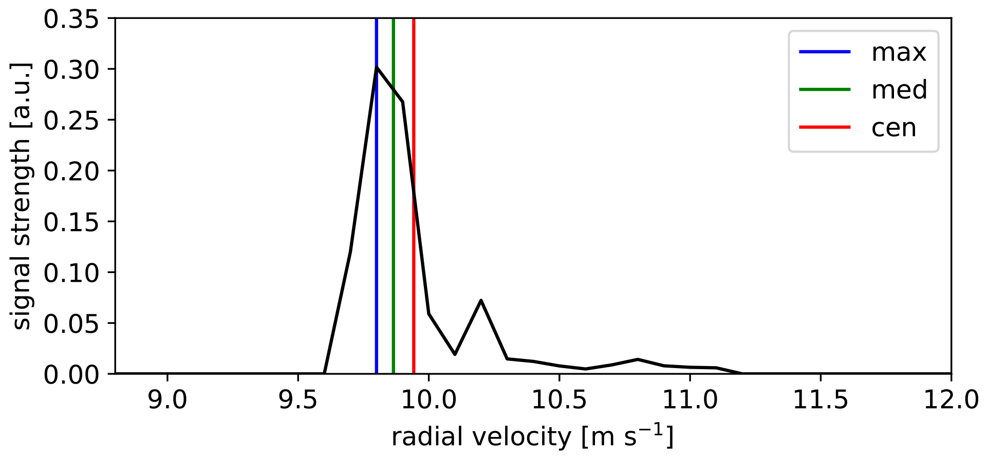
Figure 1 Example of a Doppler radial velocity spectrum simulated in a turbulence box, including the radial velocity estimates using the maximum (max), the median (med) and the centroid (cen) methods.

3 Experiment setup

3.1 Measurement campaign

A measurement campaign on a Vestas V52 wind turbine was conducted at DTU Risø campus in Roskilde, Denmark. Figure 2 shows a layout of the test site on a digital surface elevation model. The terrain is slightly hilly and the surface is characterized by a mix of cropland, grassland and coast. A row of wind turbines stands ≈200–300 m south-east of the Roskilde fjord. The V52 wind turbine (marked as a red circle) is located at the northernmost position. It has a rotor diameter D of 52 m, a hub height of 44 m and a nominal power of 850 kW. The rotor speed is within the range of 14–31 rpm with a nominal value of 26 rpm. The cut-in, rated and cut-out wind speeds are 4, 14 and 25 m s⁻¹, respectively. A meteorological mast (marked as a red square) was mounted at 291^∘ (from the north) at a distance of 120 m (2.3D) upstream from the turbine. The mast is 72 m high and instrumented with anemometers at 18, 31, 44, 57 and 70 m above the ground level (Peña et al., 2019): Metek USA-1 3D sonic anemometers are on the northern side of the booms and Risø cup anemometers on the southern side of the booms. In addition, there is a wind vane at 41 m and Risø absolute temperature sensors at 18 and 70 m. There are also a Thies precipitation opto-sensor and a Vaisala pressure sensor at 2 m (DTU Wind Energy, 2014). Three continuous-wave lidars were mounted on the nacelle of the V52 wind turbine, as shown in Fig. 3: the SpinnerLidar (on the top), a four-beam WindVision (in the middle) and a two-beam WindEye (at the bottom). The vertical displacement between the scan head of the SpinnerLidar, WindVision, WindEye and the wind turbine rotation axis is 2.47, 2 and 1.64 m, respectively. More information about the three lidars is given in Sect. 3.2.

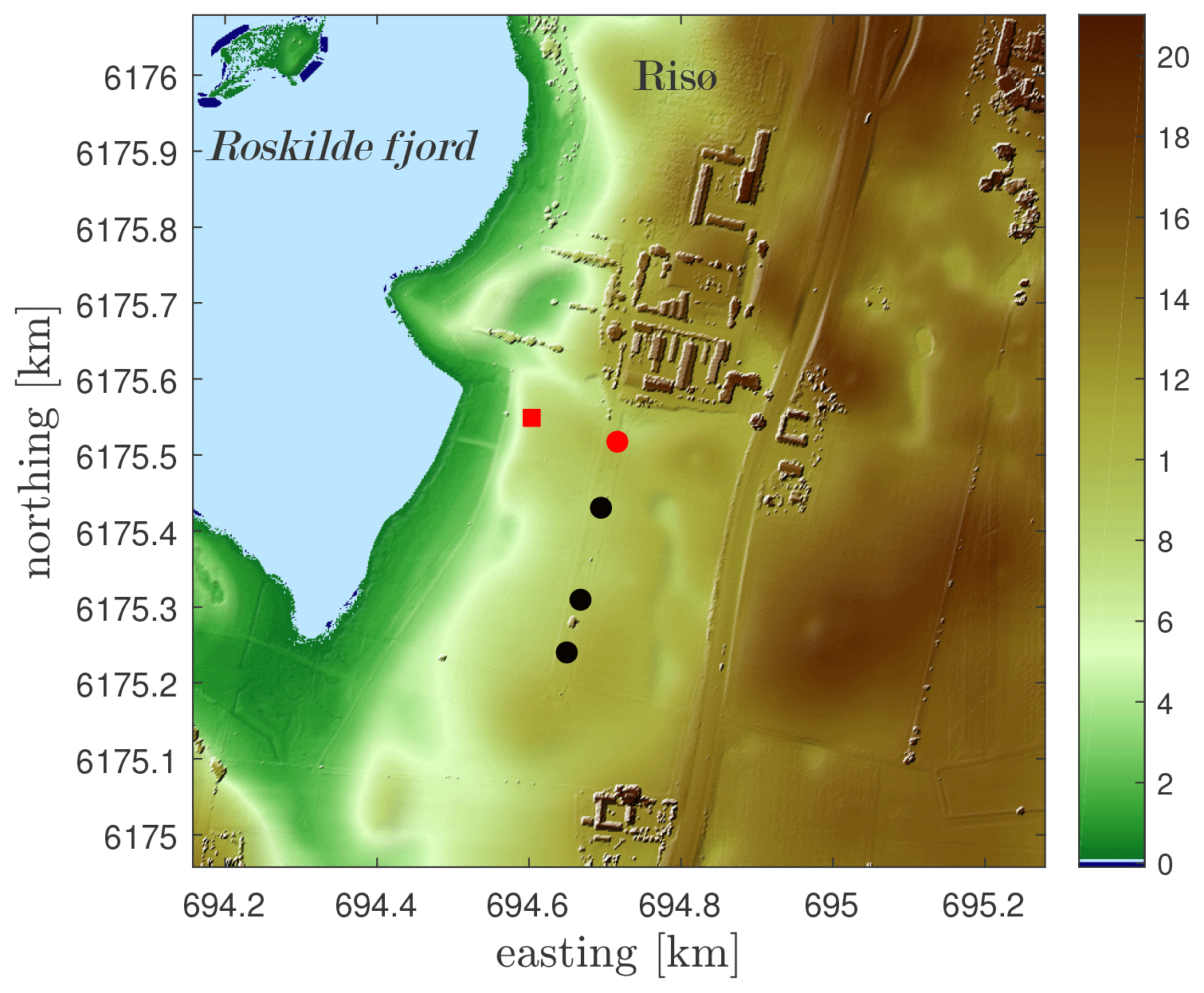
Figure 2 The Risø test site in Roskilde, Denmark, on a digital surface elevation model (UTM32 WGS84). The V52 meteorological mast is shown in a red square. The wind turbines are shown in circles (in red the reference V52 wind turbine). The color bar indicates the height above mean sea level in meters.

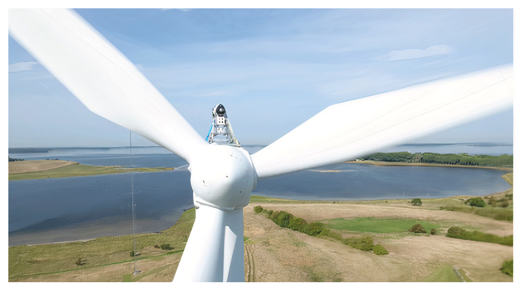
Figure 3 Three lidars sitting on the nacelle of the V52 wind turbine at DTU Risø campus: SpinnerLidar (top), WindVision (middle) and WindEye (bottom).

3.2 Nacelle lidars

Three forward-looking nacelle lidars are investigated here. All lidars are based on a CW system and they all were scanning at a single plane (see Fig. 4). The specifications for three nacelle lidars can be found in Table 1. The SpinnerLidar (Peña et al., 2019) scans in a rosette-curve pattern and generates 400 radial velocities in one full scan. For this measurement campaign, the SpinnerLidar was set up to perform a full scan every 2 s at a focus distance of 62 m. The system also recorded the instantaneous Doppler spectrum of the radial velocity, which is used here both to derive the radial velocity using different methods and to estimate the unfiltered radial velocity variance. The SpinnerLidar streams out average Doppler spectra at a rate of 200 Hz. Each Doppler spectrum is represented in 256 frequency bins with a spectral resolution of 195.3 kHz corresponding to a radial velocity resolution of 0.1528 m s⁻¹ per bin. In addition, it recorded the signal strength (here called “power”) of the instantaneous spectrum. We also use the inclination and the azimuthal positions from the SpinnerLidar sensors to correct the scanned locations.

Figure 4 (a) The scanning trajectory of the nacelle lidars. (b) An upwind view of the theoretical scanning pattern performed by the W2, W4 and the SpinnerLidar.

Table 1 Specifications of the nacelle lidars for the measurement campaign.

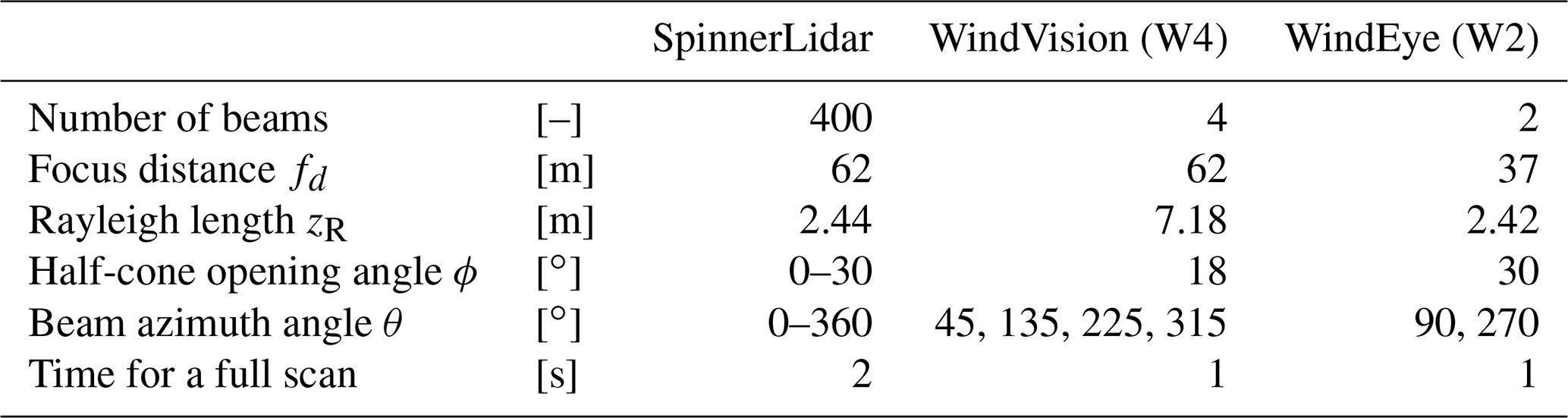
The two-beam WindEye (hereafter W2) and the four-beam WindVision (hereafter W4) are two commercial lidars from Windar Photonics A/S (Windar Photonics, 2020). W2 measured at 37 m and has similar width of the probe volume (indicated by the Rayleigh length) as the SpinnerLidar. Note that the largest probe volume and the smallest half-cone opening angle are those of the four-beam system. The azimuthal angle in Table 1 refers to the position of the beams on the scanning cone surface (from the top of the cone). The two beams from W2 are aligned horizontally, while the four beams from W4 focuses at each quadrant of the rotor area. Both systems complete a scan in 1 s.

4 Data analysis

4.1 Data selection and filtering

The measurements were collected between 1 October 2020 and 30 April 2021. We analyze the time series of all data and their statistics within 10 min periods (in total 30 492 periods of 10 min). There are three types of measurements: the supervisory control and data acquisition of the wind turbine, the mast measurements and the measurements from three lidars. We concentrate our analysis on the wind sectors, which are relatively aligned with the mast-turbine direction (291^∘) to exclude the influence of the wakes from the nearby wind turbines to the greatest extent. We select 10 min periods for the analysis using the following criteria:

• All lidars and the V52 turbine should be concurrently operating. The turbine status is indicated by the rotor speed, which should be higher than 14 rpm. This leaves us 19 190 periods of 10 min.

• The wind direction measured by the wind vane and the yaw angle of the turbine are both between 261–321^∘. The absolute difference between these two directions is lower than 5^∘. Since the dominant wind direction at this site is west and south-west, we have 2457 periods of 10 min left after applying this filter.

• The wind speed measured by the cup anemometer at the turbine hub height is higher than 3 m s⁻¹.

• No precipitation is detected during the 10 min period.

After filtering, the number of the 10 min periods for the analysis is 2348.

4.2 SpinnerLidar measurements

4.2.1 Data filtering

We process the SpinnerLidar measurements for the selected 2348 periods of 10 min. The SpinnerLidar measurements are further filtered based on both the system-reported radial velocity, which is the median estimate from the raw Doppler radial velocity spectrum, and the power of the spectrum. The following criteria are applied (Fig. 5 shows an example of results of the SpinnerLidar filtering within an arbitrary 10 min period):

• We filter out all measurements with system-reported radial velocity estimates below 3.2 m s⁻¹, which is the reference minimal detectable radial velocity by the SpinnerLidar due to the interference of the turbine blades (Karen Enevoldsen, personal communication, 2021).

• We simulate the radial velocity of all possible blade returns as (Angelou et al., 2015)

  $$\begin{array}{}\text{(27)}& v_{\mathrm{r}}=\left|\mathrm{\Omega }{S}_y{h}_{\text{SL}}\right|,\end{array}$$

  where Ω is the 10 min mean rotor speed, S_y is the lateral component of the unit vector with reference to the SpinnerLidar in the y–z plane, and h_SL is the vertical displacement between the SpinnerLidar scan head and the wind turbine rotation axis. Equation (27) does not consider the misalignment between the SpinnerLidar and the nacelle, which is negligible (below 0.5^∘) in the measurement campaign. The simulated blade signals are marked in red in Fig. 5. We discriminate the wind speed signal from the blade return signal from Eq. (27) when the difference between them is above 0.2 m s⁻¹.

• We filter out all measurements exceeding power values above 100 (Peña et al., 2019) (this signal strength has arbitrary units). We can see from Fig. 6 that some measurements close to the middle of the pattern are filtered out with this criterion.

• Finally, we filter out radial velocities exceeding its mean ± 3 times its standard deviation within the 10 min period.

Further, there should be at least half of the raw measurements left for the analysis to consider a 10 min period of SpinnerLidar measurements, which leaves us 1605 periods of 10 min for the later post-processing.

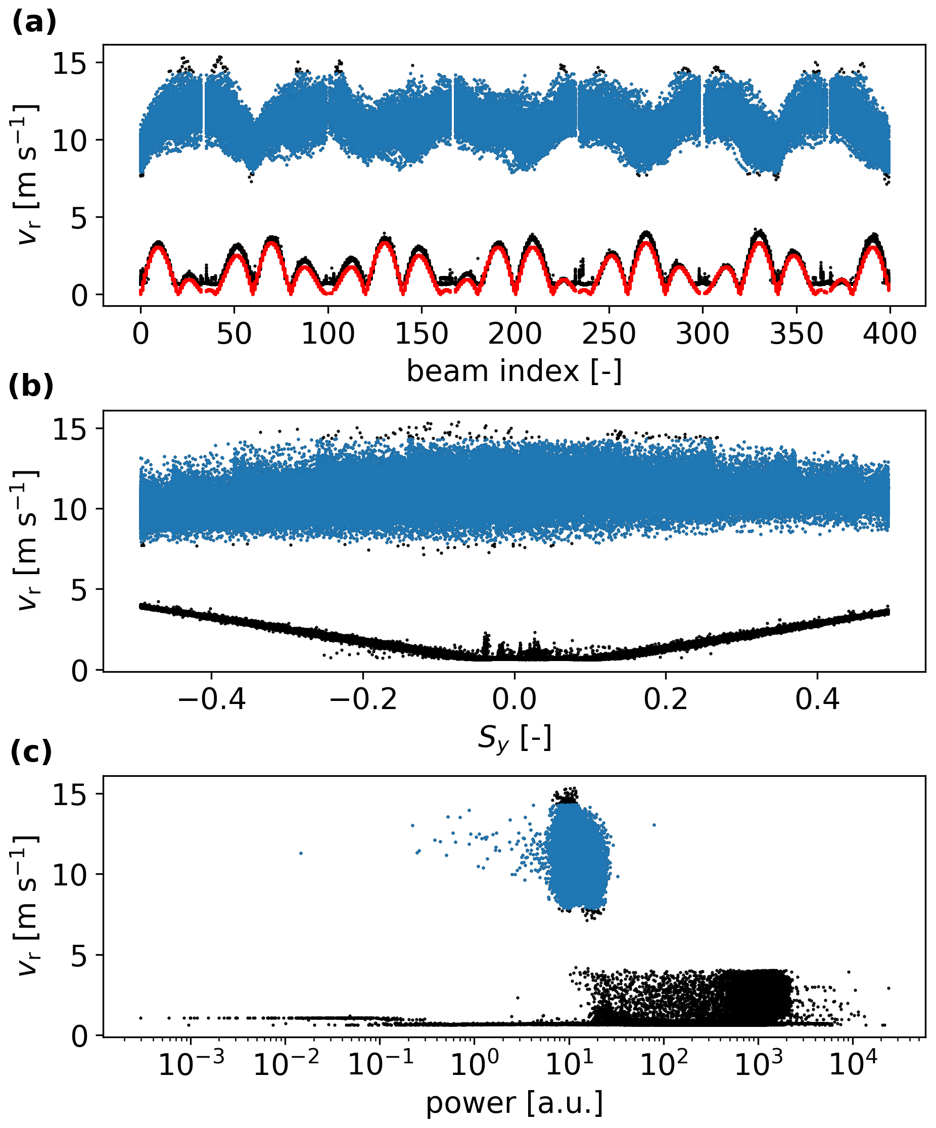
Figure 5 Radial velocity as function of (a) index of the 400 beams in each full scan, (b) the lateral component of the unit vector S_y and (c) power for an arbitrary 10 min period. Filtered data are shown in black and data left after filtering in blue. The red color in the top panel represents the simulated radial velocity from the possible blade returns.

4.2.2 Gridding the scans

We estimate the lidar scan locations using the average azimuthal and inclination angles of the SpinnerLidar within the 10 min period, i.e., the system-reported coordinates are rotated along the longitudinal and lateral axis of the SpinnerLidar scanhead, respectively. Figure 6a shows the scan locations in blue and the non-rotated locations in orange within a 10 min period (26 February 2021 at 14:10:00), where the average inclination angle is 3.15^∘ and the average azimuthal angle is 0.34^∘.

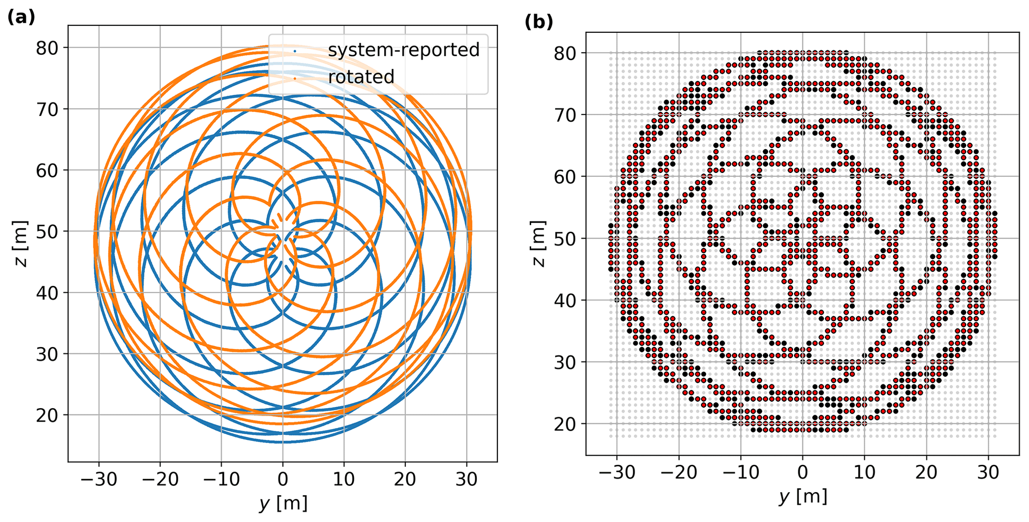
Figure 6 (a) Scan locations (before and after rotation) in an arbitrary 10 min period. (b) Gridding of the scans within the same 10 min period. Grid cells with more than 30 radial velocity spectra are marked in red. Other details are given in the text.

Due to the turbine movement and SpinnerLidar slack, we aggregate the azimuthal- and inclination-corrected scan locations within a grid of 1 m resolution in the y–z plane, as shown in Fig. 6b. The coordinates of the grid cells, which are marked in light grey, are given by the resolution and extension of the grid. The “gridded” rosette pattern is shown in black (some are covered by red color as explained later). All radial velocity spectra for the scans lying within each grid cell in the given 10 min period are accumulated. We use only grid cells, where there are more than 30 instantaneous Doppler radial velocity spectra. In Fig. 6b, we show in red the grid cells satisfying this criterion. Finally, we only use those 10 min periods in which we have 900 grid cells satisfying the criterion.

4.2.3 Doppler spectra processing and usage

Figure 7 shows an example of the processing of the Doppler radial velocity spectra from the accumulated measurements within a grid cell close to the middle of the scan. The raw Doppler radial velocity spectra within that grid cell are shown in Fig. 7a. For this 10 min period (26 February 2021 at 14:10:00), the vane measures a wind direction of 291.6^∘ and the yaw angle is 291.0^∘. The lidar unit vector pointing onto this grid cell is almost parallel to the terrain (ϕ is around 1.4^∘), thus close to the main wind direction. As shown in Fig. 7a, high spectral values “contaminate” the spectra in the first few velocity bins due to, e.g., optical reflections from the bore point (i.e., the beam hitting the telescope lens perpendicularly) or few left blade signals. To ease the spectra processing, we define a threshold for each individual spectrum, which defines the limit above which a Doppler spectrum is considered to be caused by the wind. The calculation of the threshold is based on the mean value (μ) plus a number of standard deviations (σ) within a frequency range where no radial velocity signals are anticipated. Angelou et al. (2012) showed that a systematic selection of the threshold level should take into account the shape of the Doppler spectrum relative to the variation of the spectrum noise level. The number of standard deviations is thus different for the case of a wide Doppler velocity spectrum (high turbulence level) and a narrow one (low turbulence level). An overestimation of the threshold removes low-intensity fluctuations and, subsequently, biases the estimation of the radial velocity and reduces its variance. Here, we select a threshold of μ+3σ of the spectral values in the last 50 frequency bins. After thresholding, we remove the spectral values up to the bin corresponding to 2.3 m s⁻¹, which filters out the high spectral peaks in unrealistic low-velocity bins (Fig. 7b).

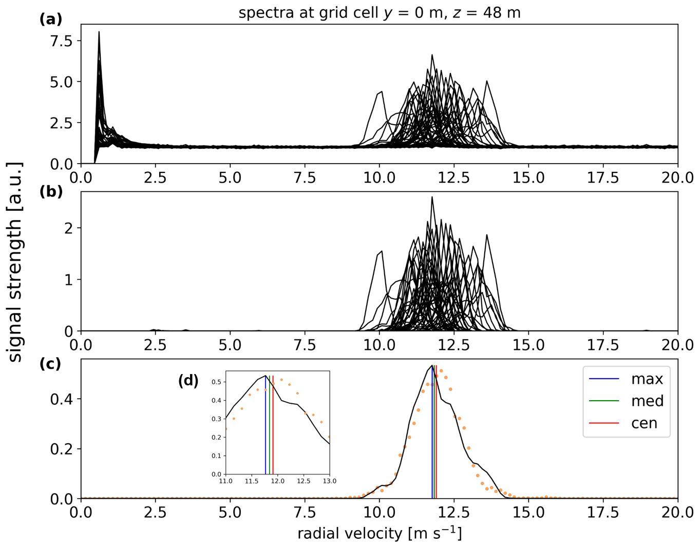
Figure 7 An example of Doppler radial velocity spectra analysis within a 10 min period (26 February 2021 at 14:10:00). The location of the grid cell y=0 m, z=48 m is shown in the scanning pattern in Fig. 6b. (a) Raw and scaled Doppler radial velocity spectra. (b) Cleaned and normalized Doppler spectra. (c) The average Doppler spectrum (black), the distribution of the sonic measurements at hub height (orange) and the three radial velocity estimates, which can be clearly seen in the inset (d).

Each “cleaned” spectrum is then area-normalized. Figure 7c shows the ensemble-average Doppler radial velocity spectrum from all normalized, thresholded and cleaned spectra. We also show the normalized distribution of sonic measurements at hub height within the same 10 min period projected to the direction of the grid cell unit vector, which as illustrated are in good agreement with the ensemble-average Doppler radial velocity spectrum. We use the ensemble-averaged Doppler radial velocity spectrum to derive both the unfiltered radial velocity variance and the radial velocity estimates (maximum, centroid and median), which are later used for the reconstruction of the mean wind.

All grid cells with at least 900 Doppler radial velocity spectra within each 10 min period are considered for the reconstruction of the mean wind and the Reynolds stresses. The three-dimensional mean wind vector is computed from the median-, maximum- and centroid-radial velocities, using the approach in Sect. 2.5.1. Figure 8a shows a contour map of the median-derived radial velocity for an arbitrary 10 min period of SpinnerLidar measurements. As expected, the highest radial velocities are found in the middle-top part of the scan. This radial velocity contour map shows a similar pattern as that from the average of SpinnerLidar simulations using 30 turbulence boxes (Fig. 8b).

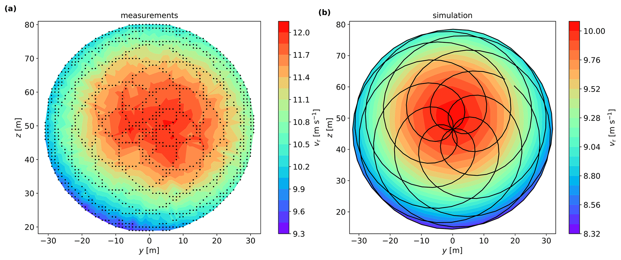
Figure 8 (a) Contour map of the median-derived radial velocity from the ensemble-average Doppler spectra in a 10 min period. Black dots indicate the location of the grid cells with more than 30 Doppler spectra. (b) Contour map of the average median-derived radial velocity from SpinnerLidar simulations using 30 turbulence boxes.

4.3 Windar measurements

4.3.1 Data filtering

The measurements for the W2 and W4 nacelle lidars are processed at 2 and 4 Hz, respectively. Therefore, within a 10 min period, the optimal amount of radial velocities per beam for W2 is 1200 and for W4 is 2400. We remove outliers of radial velocities and apply the same blade filtering using the method described in Sect. 4.2. We set a criterion that there should be at least 90 % of the optimal amount of data left after the filtering for a 10 min period. We do not account for the radial velocities of a full scan when data from any beam are missing. This leaves us 1499 periods of 10 min for the intercomparison.

4.3.2 Methods to compute the along-wind velocity variance

The along-wind and lateral velocities are reconstructed for each scan (i.e., for every 1 s) using the approach described in Sect. 2.5.2, and we compute 10 min statistics from these velocities. Due to the limited number of beams and the unavailability of Doppler radial velocity spectra, we only compute the filtered along-wind variance using two methods. We can compute the wind speed variance directly from the time series of reconstructed along-wind velocity U within the 10 min periods (hereafter denoted as the “U-variance” method). We can also compute ${\mathit{\sigma }}_u^{\mathrm{2}}$ using Eq. (23) with some assumptions and three are investigated here. The first is to assume that all Reynolds stress components apart from ${\mathit{\sigma }}_u^{\mathrm{2}}$ are zero (hereafter denoted as the “LSP-${\mathit{\sigma }}_u^{\mathrm{2}}$” method). This basically means that Eq. (23) becomes

$$\begin{array}{}\text{(28)}& {\mathit{\sigma }}_u^{\mathrm{2}}={\displaystyle \frac{{\mathit{\sigma }}_{v_{\mathrm{r}}}^{\mathrm{2}}}{{\cos }^{\mathrm{2}}\mathit{\varphi }}}.\end{array}$$

Since the half-cone opening angle of nacelle lidars is usually small, this method tends to overestimate ${\mathit{\sigma }}_u^{\mathrm{2}}$. The second is to assume turbulence isotropy; i.e., the auto-variance of the three velocity components is the same and they are uncorrelated (hereafter denoted as the “LSP-isotropy” method). From Eq. (23), this means that ${\mathit{\sigma }}_u^{\mathrm{2}}$ is then the average of the radial velocity variances of the lidar beams. The third option is to assume that σ_v=0.7σ_u and σ_w=0.5σ_u, as suggested in IEC (2019) (hereafter denoted as the “LSP-IEC” method).

4.4 Sonic measurements

We use the 20 Hz raw sonic measurements at hub height (44 m) to calculate the mean horizontal wind speed and its variance for all selected 10 min periods. Figure 9a shows that the horizontal speed measured by the cup and the sonic anemometer is nearly the same. When looking at the computed variance in Fig. 9b, a bias of 3.4 % is found. We rotate the sonic-measured 3-D wind components, which are defined in the main wind coordinate system, to the coordinate system fixed with the wind turbine so that the sonic u velocity is aligned with the rotation axis of the turbine. We use the velocity and the variance of the rotated sonic-measured mean wind components as the reference for the comparison with the estimates from the nacelle lidars.

Figure 9 Comparison of the 10 min mean horizontal (a) wind speed and (b) variance between the sonic and the cup anemometers at 44 m. Each 10 min is shown in blue markers, a 1:1 relation is shown in the red dashed line, and a linear regression fit to origin in the black dashed line (results of the regression are given on the top of the plot, where R² is the coefficient of determination).

5 Results

5.1 Mean wind speed

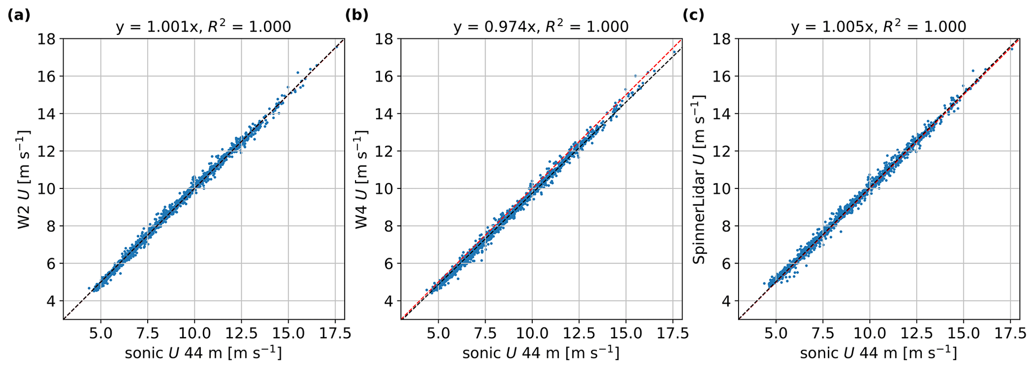
We perform comparisons of the 1499 10 min mean along-wind velocity component reconstructed from the lidar measurements with that from sonic measurements at 44 m (see Fig. 10). The estimates from lidars and the sonic anemometer are corrected for the induction using the method in Sect. 2.5.3. The lidar-derived estimate is a rotor-effective mean velocity since measurements at all scanning positions are considered. As illustrated, there is a high correlation for all nacelle lidars, as expected. The W2 and the SpinnerLidar estimates are slightly higher than that from the sonic anemometer while the estimate of W4 is 2.6 % lower. From the numerical simulation with 30 turbulence boxes, we found that all nacelle lidars are able to estimate the along-wind velocity well (not shown here); the uncertainties in the mean wind obtained from lidar are as large as those from the sonic anemometer.

Figure 10 Comparison between the reconstructed along-wind mean velocity from the sonic anemometer at 44 m and (a) W2, (b) W4 and (c) SpinnerLidar. All estimates are corrected for the induction. Features regarding the red and black dashed lines as in Fig. 9.

5.2 Radial velocity variance

Figure 11a shows the simulated ratio of the unfiltered radial velocity variance to the u-velocity variance of the sonic anemometer among the scanning area. As the simulated wind field is based on the Mann model, the major source of cross-contamination on the radial velocity comes from the spectral tensor components involving w. As seen from the plot, the ratio is higher than one above the center and lower than one beneath it, which is due to the positive and negative contribution of $\langle u^{\prime }{w}^{\prime }\rangle$, respectively, to the beam radial variance. Figure 11b shows the result from the measurement campaign as a scatter plot between the unfiltered radial velocity variance of the central grid cell (y=0 m, z=48 m) from the SpinnerLidar to the u variance of the sonic anemometer measurements at 44 m. From the measurements, the unfiltered radial velocity variance of the central beam reaches 91.5 % of the sonic variance, whereas the simulations show a zero bias for that central beam. We attribute this difference to our rather conservative method to clean Doppler radial velocity spectra, which attempts to eliminate any possible noise. However, this might lead to reduction of true turbulence contained in the Doppler radial velocity spectrum.

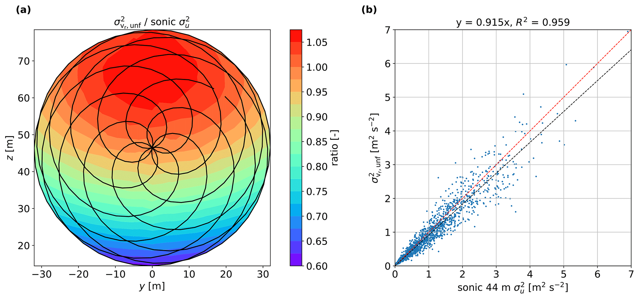
Figure 11 (a) Ratio of the unfiltered radial velocity variance to the u-velocity variance of the sonic anemometer from the simulations (30 turbulence boxes are used). (b) Comparison between the unfiltered radial velocity variance at the central grid cell (y=0 m, z=48 m) and the u variance of the sonic anemometer at 44 m from the measurements. Features regarding the red and black dashed lines as in Fig. 9.

In Fig. 12a, we show the probe volume filtering effect on the scanning pattern by plotting the ratio of the filtered to the unfiltered radial velocity variance from the simulations. Here, the filtered radial velocity variance is computed from the centroid-derived radial velocity, because the centroid method experiences the most turbulence attenuation caused by the probe volume (Held and Mann, 2018). The filtering effect due to probe volume is very similar throughout the pattern. The highest ratios are found around the center of the pattern, where the beam aligns with the along-wind velocity component. As the beam moves from the center, the ratio decreases because the beam's opening angle increases and the cross-contamination from other velocity components increases. The amount of the cross-contamination depends highly on the anisotropy of turbulence Γ. Our simulation was conducted with a set of typical Mann parameters (see Sect. 2.7), so the degree of simulated filtering can be different from that of measurements. Figure 12b shows the comparison between the filtered and unfiltered radial velocity variance at the grid cell (y=0 m, z=48 m) from the measurement campaign. The correlation is very high, as expected, and the unfiltered radial velocity variance is around 9 % higher than the centroid-derived filtered one.

Figure 12 (a) Ratio of the filtered to the unfiltered radial velocity variance from simulations (30 turbulence boxes are used). (b) Comparison between the SpinnerLidar filtered and unfiltered radial velocity variance at the central grid cell (y=0 m, z=48 m) from the measurements. Features regarding the red and black dashed lines as in Fig. 9.

5.3 Turbulence estimates

Using the methodology described in Sect. 2.6, we estimate the six components of the Reynolds stress tensor from the SpinnerLidar unfiltered radial velocity variances and compare them against the computed components from the sonic anemometer measurements at 44 m for the 1499 periods of 10 min. Figure 13 shows the inter-comparison for ${\mathit{\sigma }}_u^{\mathrm{2}}$. From the simulation with 30 turbulence boxes, we get a nearly perfect correlation and a bias of 1.4 %, whereas from the measurements the bias is 8.9 %. The bias is higher in the measurements mainly because we cannot guarantee that some variance of the radial velocity is lost when processing the Doppler radial velocity spectra.

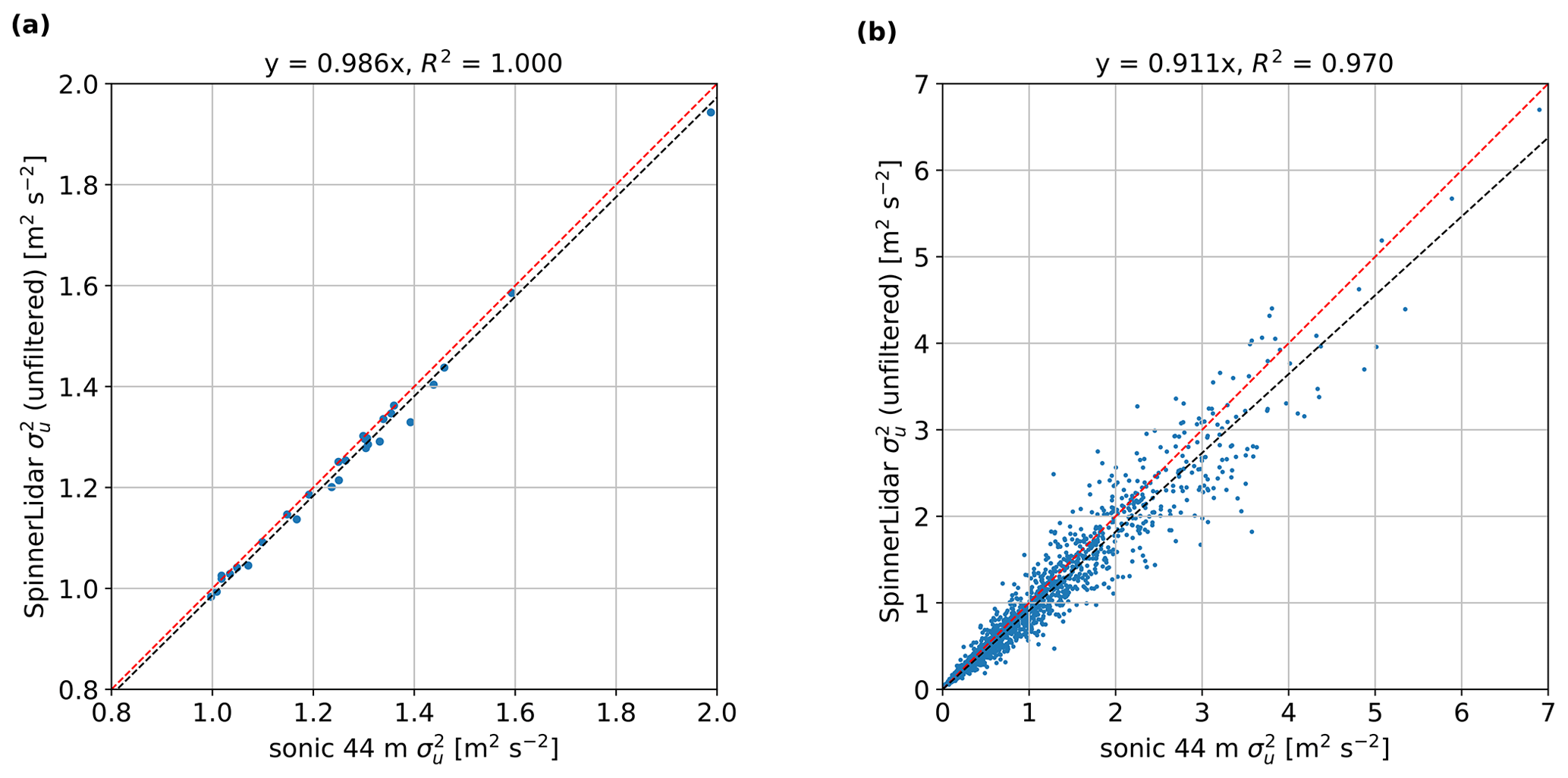
Figure 13 Comparison of the unfiltered variance of the along-wind velocity component between the SpinnerLidar and the sonic anemometer at 44 m from (a) numerical simulation using 30 turbulence boxes and (b) measurement campaign.

We perform the comparison of all Reynolds stresses computed from the SpinnerLidar scans with those from the sonic anemometer at 44 m in Fig. 14. The Reynolds stresses from the measurement campaign are normalized by U² with which they are roughly proportional. The unfiltered variances from simulations were derived by the same method (see Sect. 2.4) as for the measurements. The numerical simulations show that we can accurately estimate all components of the Reynolds stress tensor using the SpinnerLidar compared to the sonic anemometer. The SpinnerLidar uncertainties of $\langle u^{\prime }{u}^{\prime }\rangle$ are not very different from those of the sonic anemometer, while the uncertainties of other components are larger. This is mainly because all other components where u fluctuations are not included are driven by fluctuations of components largely misaligned with the beams. Results from the measurements show that all Reynolds stress components estimated from SpinnerLidar are close to those from the sonic anemometer but biased. We even observe negative values for $\langle v^{\prime }{v}^{\prime }\rangle$ and $\langle w^{\prime }{w}^{\prime }\rangle$. This is discussed in Sect. 6.2.

Figure 14 Reynolds stresses derived from the SpinnerLidar and sonic anemometer, (a) numerical simulations using 100 turbulence boxes and (b) measurements. The markers are the means and the error bars are ± 1 standard deviation.

Figure 15 shows the comparison of the SpinnerLidar estimations of the maximum-, median- and centroid-derived filtered variances of the along-wind velocity component with those from the 44 m sonic measurements. Results from both the simulations using 30 turbulence boxes and the measurements indicate that turbulence attenuation is most severe using the centroid method from the Doppler radial velocity spectrum, while the maximum method gives the closest value, as expected (Held and Mann, 2018).

Figure 15 Comparison of the filtered variance of the along-wind velocity component between the SpinnerLidar and the sonic anemometer at 44 m. (a–c) Numerical simulations using 30 turbulence boxes. (d–f) Measurement campaign.

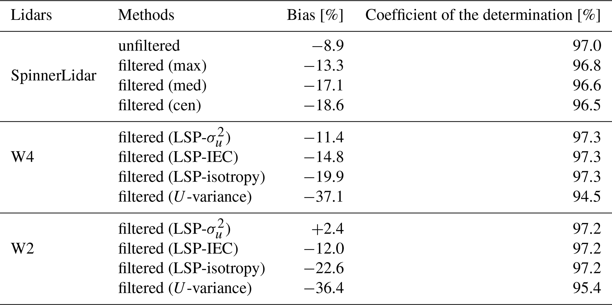
Figure 16 shows the comparison of the Windar lidar reconstructed filtered ${\mathit{\sigma }}_u^{\mathrm{2}}$ using different methods against ${\mathit{\sigma }}_u^{\mathrm{2}}$ values from the 44 m sonic anemometer. As illustrated, about 37 % of the variance is filtered out for both W4 and W2, when the variance is computed by taking the statistics of the reconstructed U time series. This is still the common practice in the wind energy community. The degree of filtering is similar for both lidars although W4 has a larger probe volume. From Eq. (28), we note that by using the “LSP-${\mathit{\sigma }}_u^{\mathrm{2}}$” method, we can overestimate the along-wind variance when all beams are scanning horizontally (or close to). Estimates using the “LSP-isotropy” method take the average of all beam variances. When the scanning geometry is symmetrical in the two-dimensional y–z plane (like in the W4 case), the contributions from $\langle u^{\prime }{w}^{\prime }\rangle$ might (nearly) cancel out. The method “LSP-IEC” is perhaps a fairer procedure when compared to the other methods, as it assumes relations between velocity components' variances that are close to those we can observe within the atmospheric surface layer. Estimates from the “LSP-IEC” and “LSP-isotropy” methods can be computed by scaling those from method “LSP-${\mathit{\sigma }}_u^{\mathrm{2}}$”; that explains the same correlations in Fig. 16a–c and e–g. All inter-comparison results of the estimated along-wind components are summarized in Table 2.

Figure 16 Comparison of the filtered variance of the along-wind velocity component between the Windar lidars and the sonic anemometer at 44 m. (a–d) W4. (e–h) W2.

Table 2 Bias and coefficient of determination between the lidar-derived along-wind velocity variance using different lidars and methods and that from the sonic anemometer at 44 m.

6 Discussion

6.1 Influence of spectra processing on the unfiltered variances

The way we process the Doppler radial velocity spectra influences the unfiltered variance estimates. Therefore, we investigate the sensitivity of using a more rigorous method to further alleviate the contamination of the Doppler spectra from, e.g., noise. This method first determines the peak of the Doppler signal and then moves forwards and backwards in the vicinity of the peak velocity bin to find the two locations (velocity bins) where the Doppler signal reaches zero. Only Doppler signals between these two velocity bins are used to compute the variance. The unfiltered along-wind velocity variance estimated from the SpinnerLidar measurements shows a bias reduction of ≈3.0 % using the more rigorous spectra-processing when compared to the relatively “moderate” method, which is used in Sect. 4.2.3. The coefficient of the determination reduces from 97 % to 96.6 %.

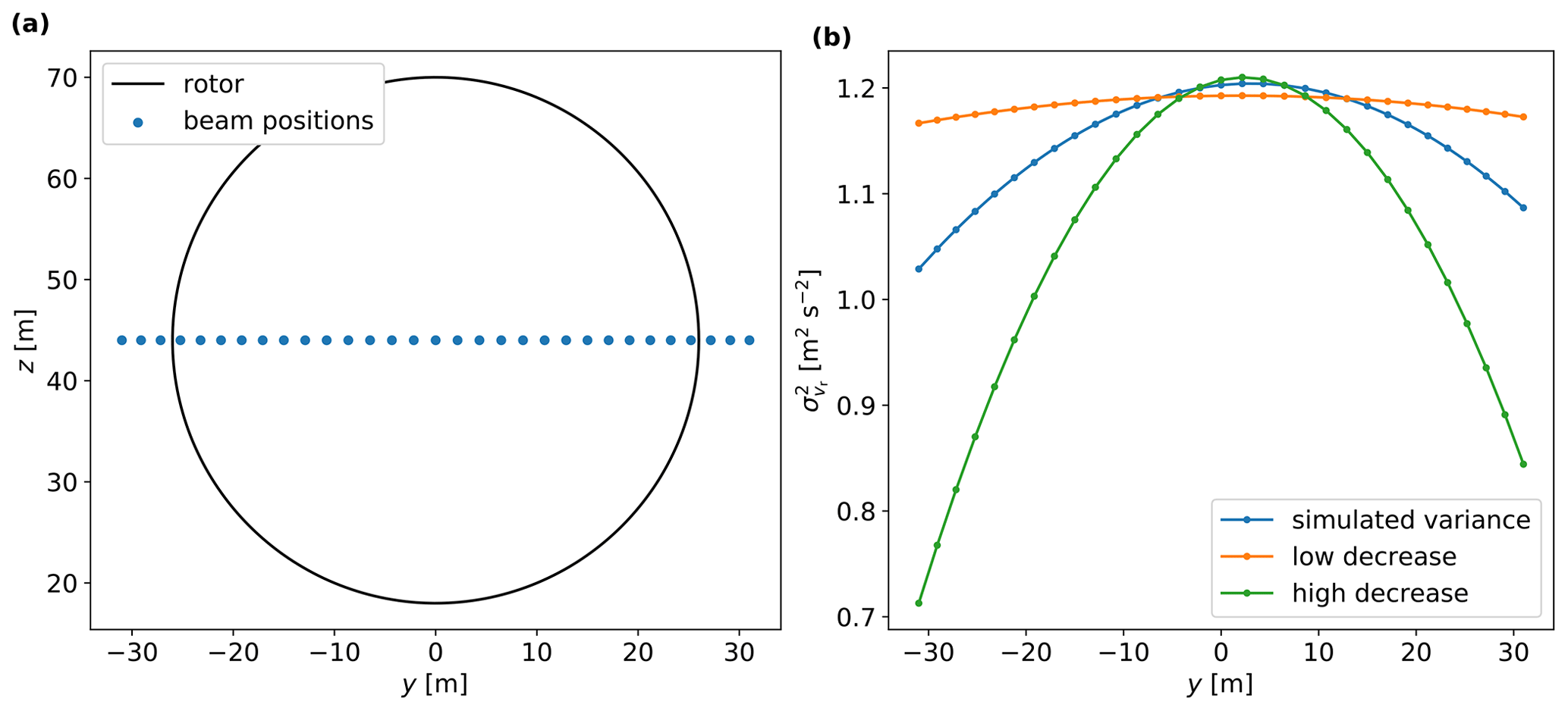
Figure 17 (a) Scanning pattern of a nacelle lidar with beams across the rotor. (b) The radial velocity variances of the beams across the rotor from simulations using five turbulence boxes.

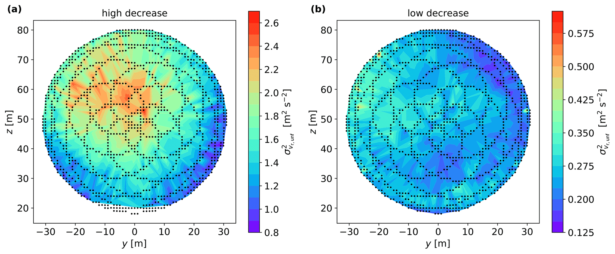
Figure 18 Contour plots of the radial velocity variance over the SpinnerLidar scanning pattern during two 10 min periods, (a) a case with negative ${\mathit{\sigma }}_v^{\mathrm{2}}$ and ${\mathit{\sigma }}_w^{\mathrm{2}}$ values, (b) a case with ${\mathit{\sigma }}_u^{\mathrm{2}}\approx {\mathit{\sigma }}_v^{\mathrm{2}}>{\mathit{\sigma }}_w^{\mathrm{2}}$.

6.2 Negative SpinnerLidar-derived variances

Negative variances might result when using SpinnerLidar measurements to estimate the Reynolds stress tensor. We find randomly occurring negative values of ${\mathit{\sigma }}_v^{\mathrm{2}}$ in 7 % and of ${\mathit{\sigma }}_w^{\mathrm{2}}$ in 15 % of the 10 min periods that are used for the inter-comparison. We investigate the conditions in which this occurs by simulating measurements of a nacelle lidar with 30 beams such that they cover the extent of rotor at hub height (see Fig. 17a). Figure 17b shows the simulated radial velocity variances (marked in blue) of the beams across the rotor. Each point corresponds to the average radial velocity variance from five turbulence fields. With increasing opening angle, the simulated radial velocity variance decreases. By using the method in Sect. 2.6 to derive the velocity variances, we obtain positive values of all velocity components and ${\mathit{\sigma }}_u^{\mathrm{2}}\gg {\mathit{\sigma }}_v^{\mathrm{2}}$, as expected. We obtain negative ${\mathit{\sigma }}_v^{\mathrm{2}}$ values when the radial velocity variances highly decrease with increasing opening angle (high decrease marked in green in Fig. 17b). In this case, the turbulence homogeneity assumption is not satisfied. Further, we find ${\mathit{\sigma }}_u^{\mathrm{2}}\approx {\mathit{\sigma }}_v^{\mathrm{2}}$ when ${\mathit{\sigma }}_{v_{\mathrm{r}}}^{\mathrm{2}}$ slowly decreases with increasing opening angle (low decrease). Figure 18a shows the pattern of unfiltered radial velocity variances in one of the 10 min periods where we estimate negative ${\mathit{\sigma }}_v^{\mathrm{2}}$ and ${\mathit{\sigma }}_w^{\mathrm{2}}$ variances. As illustrated, the pattern shows a strong decrease of ${\mathit{\sigma }}_{v_{\mathrm{r}}}^{\mathrm{2}}$ particularly around the right side of the scans. Figure 18b corresponds to another 10 min period where ${\mathit{\sigma }}_u^{\mathrm{2}}\approx {\mathit{\sigma }}_v^{\mathrm{2}}>{\mathit{\sigma }}_w^{\mathrm{2}}$. The occurrence of the negative variances is less frequent in our measurements when we perform the turbulence estimation every 30 min, as expected.

7 Conclusions

In this study, we analyzed measurements of three forward-looking nacelle lidars with different scanning configurations to investigate the benefit of multi-beam nacelle lidars for turbulence characterization. For the first time, the SpinnerLidar measurements were compared with those of commercial nacelle lidars. We focused our analysis on wind sectors, in which the inflow is relatively homogeneous. The inflow characteristics estimated by three lidars were compared with those from a nearby sonic anemometer at hub height.

Our results from the analysis of numerical simulations and measurements showed that all lidars were able to estimate the mean wind velocity well compared to the sonic anemometer. We also found that the SpinnerLidar was the only one out of the three nacelle lidars that is able to measure the six Reynolds stress components accurately. This is due to both its multi-beam capability and its ability to measure unfiltered radial velocity variances.

By using the information from the Doppler radial velocity spectrum, one can partly compensate for the probe volume averaging effect and reduce the error of turbulence estimation. We showed that using maximum-derived radial velocities to compute the along-wind velocity variance mitigates best the turbulence attenuation caused by the lidar probe volume.

For the commercial lidars, one can estimate the along-wind velocity variance using three different methods: scaling the radial velocity variance with a factor of cos ²ϕ, assuming σ_v=0.7σ_u and σ_w=0.5σ_u, or assuming isotropic turbulence. We found the smallest bias in the estimates using the first method when compared to the sonic anemometer values. However, the first method can overestimate the along-wind variance when all beams are scanning horizontally. The second method is the fairest procedure among the three methods. All methods showed smaller bias when compared to computing the variance from the reconstructed along-wind velocity values in the time series.