Generalized analytical body force model for actuator disc computations of wind turbines

A new generalized analytical model for representing body forces in numerical actuator disc models of wind turbines is proposed and compared to results from a blade element momentum (BEM) model. The model is an extension of a previously developed load model, which was based on the rotor disc being subject to a constant circulation, modified for tip and root effects, corresponding to an optimum design case. By adding a parabolic circulation distribution, corresponding to a solid-body approach of the flow in the near wake, it is possible to take into account losses associated with off-design cases, corresponding to pitch regulation at high wind speeds. The advantage of the model is that it does not depend on any detailed knowledge concerning the actual wind turbine being analysed but only requires information about the thrust coefficient and tip-speed ratio. The model is validated for different wind turbines operating under a wide range of operating conditions. The comparisons show generally an excellent agreement with the BEM model even at very small thrust coefficients and tip-speed ratios.

1 Introduction

The actuator disc concept has for many years been employed as a means to include body forces into the Navier–Stokes equations for rotor computations of both single rotors (e.g. Sørensen and Myken, 1992; Sørensen and Kock, 1995; Ammara et al., 2002; Mikkelsen, 2003; Jimenez et al., 2007) and multiple rotors operating in wind farms (e.g. Porté-Agel et al., 2011; Nilsson et al., 2014; Stevens et al., 2018). The simplest way of implementing body forces in the Navier–Stokes equations is to let them be prescribed either as constant loadings (Sørensen et al., 1999) or as prescribed radial distributions (Simisiroglou et al., 2016). However, if more detailed information regarding load distributions is required, it is needed to know the actual rotor geometry, i.e. the twist and chord distributions, as well as airfoil type at each cross section, including the lift and drag characteristics of the airfoils (Sørensen and Kock, 1995; Wu and Porté-Agel, 2011). Besides this, it also requires information regarding the operational envelope of the rotor, i.e. the collective pitch setting of the rotor blade and tip-speed ratio as function of incoming wind speed. In many cases, however, this information is not known, either because geometry and airfoil data are confidential or simply because the developer has not yet decided size and type of the turbines in the initial development phase of a wind farm. There is therefore a need for a method that in a simple way may represent the rotor loading by body forces without prior knowledge of the wind turbine.

A systematic study on different ways to include body forces was carried out by van der Laan et al. (2015), who showed that knowing the details of the actual loading results in a more reliable computation of the wake than simply assuming some more or less arbitrary shapes. In this study, a load model was proposed based on using the dimensionless load data from a known wind turbine to scale the loading for other turbines. Such a method actually indicates that, in dimensionless form, the rotor loading from one turbine is not very different from any other turbine. This assumption also forms the background for the analytical load model proposed by Sørensen et al. (2019). The model of Sørensen et al. (2019) is based on the assumption that, except near to root and the tip, the circulation is constant along the rotor blade. This makes it possible to derive an analytical set of equations describing axial and tangential load distributions along the blade that only depends on tip-speed ratio and thrust coefficient. As a part of the model, the load at the tip is modified by the usual tip correction (Glauert, 1935), and the root is corrected by a polynomial. The model was validated using large-eddy simulation (LES) actuator disc computations of the Tjæreborg turbine and the DTU 10 MW reference rotor operating at wind speeds corresponding to the design conditions. A further study employing the model on commercial wind turbine rotors operating at off-design conditions was recently performed by Sørensen and Andersen (2020). The studies showed that the analytical model performs excellently at design wind speeds (i.e. at wind speeds below the rated), whereas the load distributions start to deviate from the reference distributions when operating the turbine away from the design load case. To complete the analytical load model to cope with the full range of wind speeds encountered by a wind turbine, there is therefore a need for a generalized extended version of the model. The aim of the present investigation is to devise a technique to extend the analytical load model to comprise wind turbines running under different operating regimes, including off-design conditions.

The paper is organized as follows. In Sect. 2, the idea behind the analytical model is explained, and the resulting set of equations is derived. Section 3 contains a verification and tuning of the model parameters, and in Sect. 4 results are presented and discussed. Section 5 contains a discussion of the results, and the conclusion is given in Sect. 6.

2 Methodology

In this section the derivation of the analytical body force model will be described in detail. First, the control strategy of a modern wind turbine is introduced in order to state the background for the extended version of the model, and next the equations forming the analytical load model will be derived.

2.1 Power and thrust coefficients

To derive an analytical load model that is applicable for all wind speeds, it is required to understand the control strategy of a modern wind turbine. Most turbines of today are tip-speed regulated at wind speeds ranging from the cut-in wind speed to the rated wind speed, which is the wind speed where the produced power becomes equal to the installed generator power. At higher wind speeds, the rotor is pitch regulated in order to keep a constant power output. This involves turning the rotor blades about their long axis using an active control system that senses the blade position and at the same time measures the produced power to give the appropriate instructions for changing the blade pitch. The idea of pitch regulation is to limit the lift by locally decreasing the angles of attack on the blade.

As shown by Sørensen and Larsen (2021), the power production of a wind turbine at a given ambient mean wind speed, U₀, below rated wind speed may be approximated by the following generic expression:

$$\begin{array}{}\text{(1)}& P\left(U_{\mathrm{0}}\right)=\mathit{\alpha }{U}_{\mathrm{0}}^{\mathrm{3}}+\mathit{\beta },\end{array}$$

where the coefficients α and β are determined as

$$\begin{array}{}\text{(2)}& \mathit{\alpha }={\displaystyle \frac{P_{\mathrm{G}}}{U_{\mathrm{r}}^{\mathrm{3}}-U_{\mathrm{in}}^{\mathrm{3}}}},\mathit{\beta }=-{\displaystyle \frac{P_{\mathrm{G}}{U}_{\mathrm{in}}^{\mathrm{3}}}{U_{\mathrm{r}}^{\mathrm{3}}-U_{\mathrm{in}}^{\mathrm{3}}}},\end{array}$$

where P_G denotes the rated (installed) generator power, U_in is the cut-in wind speed, and U_r is the rated wind speed. This expression obviously allows for zero turbine production at the cut-in wind speed. The thrust and power coefficient are defined as

$$\begin{array}{}\text{(3)}& C_{\mathrm{T}}\equiv {\displaystyle \frac{T}{\mathrm{1}/\mathrm{2}\mathit{\rho }{A}_{\mathrm{R}}{U}_{\mathrm{0}}^{\mathrm{2}}}},C_{\mathrm{P}}\equiv {\displaystyle \frac{P}{\mathrm{1}/\mathrm{2}\mathit{\rho }{A}_{\mathrm{R}}{U}_{\mathrm{0}}^{\mathrm{3}}}},\end{array}$$

where T is the axial force, or thrust, acting on the rotor; P is the power generated by the rotor; ρ is the air density; and $A_{\mathrm{R}}=\frac{\mathit{\pi }}{\mathrm{4}}{D}^{\mathrm{2}}$ is the rotor area, with D denoting the rotor diameter. We assume that the wind turbine operates at its optimum (rated) condition, $C_{\mathrm{P}}=C_{\mathrm{P},\mathrm{r}}\left(\equiv \frac{P_{\mathrm{G}}}{\mathrm{1}/\mathrm{2}\mathit{\rho }{A}_{\mathrm{R}}{U}_{\mathrm{r}}^{\mathrm{3}}}\right)$, at wind speeds lower than the rated wind speed, U_r, and at a constant power yield, P=P_G, at wind speeds higher than the rated wind speed. This operational strategy is typical for a modern wind turbine, which is operated with a variable tip speed at wind speeds below the rated one and which is pitch regulated at higher wind speeds. An example of this is illustrated in Fig. 1, which shows the performance curve of a 1500 kW UP1500-86 wind turbine from Guodian United Power. It is seen here that the change from tip-speed regulation to pitch regulation takes place at a wind speed of about 10 m s⁻¹.

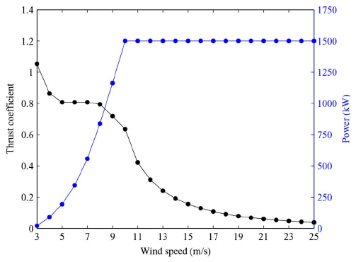
Figure 1 Typical power and thrust coefficient curves for a modern (1500 kW) wind turbine (from Gu et al., 2015).

The rated wind speed is determined from Eq. (3) at the condition where the generator operates at both maximum power and maximum (rated) power coefficient,

$$\begin{array}{}\text{(4)}& U_{\mathrm{r}}=\sqrt[\mathrm{3}]{{\displaystyle \frac{\mathrm{8}{P}_{\mathrm{G}}}{\mathit{\rho }\mathit{\pi }{D}^{\mathrm{2}}{C}_{\mathrm{P},\mathrm{r}}}}}.\end{array}$$

With the above-given assumptions, the wind turbine power curve is expressed as

$$\begin{array}{}\text{(5)}& P\left(U_{\mathrm{0}}\right)=\left\{\begin{array}{ll}\mathit{\alpha }{U}_{\mathrm{0}}^{\mathrm{3}}+\mathit{\beta };& U_{\mathrm{in}}\le U_{\mathrm{0}}<U_{\mathrm{r}}\\ P_{\mathrm{G}};& U_{\mathrm{r}}\le U_{\mathrm{0}}\le U_{\mathrm{out}}\end{array}\right.,\end{array}$$

where the wind turbine cut-out wind speed is denoted as U_out. The corresponding thrust coefficient, C_T, is approximated as

$$\begin{array}{}\text{(6)}& C_{\mathrm{T}}=\left\{\begin{array}{ll}{C}_{\mathrm{T},\mathrm{r}};& U_{\mathrm{in}}\le U_{\mathrm{0}}<U_{\mathrm{r}}\\ C_{\mathrm{T},\mathrm{r}}\cdot {\left(U_{\mathrm{0}}/U_{\mathrm{r}}\right)}^{-\mathrm{3.2}};& U_{\mathrm{r}}\le U_{\mathrm{0}}\le U_{\mathrm{out}}\end{array}\right..\end{array}$$

From this expression, it is seen that the thrust coefficient for $U_{\mathrm{r}}\le U_{\mathrm{0}}\le U_{\mathrm{out}}$ decreases with the wind speed to the power of −3.2. This value was recently derived analytically in a work by van der Laan et al. (2022). If not known in advance, typical values such as $C_{\mathrm{T},\mathrm{r}}=\mathrm{0.8}$ and $C_{\mathrm{P},\mathrm{r}}=\mathrm{0.48}$ may be employed to characterize the wind turbine performance of an actual wind turbine.

2.2 Basic equations of the load model

Applying the Bernoulli equation in a rotating frame of reference across the rotor plane, we get the following expression for the pressure drop over the rotor disc (see Glauert, 1935 or Sørensen, 2016):

$$\begin{array}{}\text{(7)}& \mathrm{\Delta }p=\mathit{\rho }\mathrm{\Omega }r{u}_{\mathit{\theta }}+\mathrm{1}/\mathrm{2}\mathit{\rho }{u}_{\mathit{\theta }}^{\mathrm{2}},\end{array}$$

where Ω is the angular velocity of the rotor, u_θ is the azimuthal velocity in the wake just behind the rotor, and r is the radial distance to the point considered. From this equation and the moment of momentum equation, sometimes referred to as Euler's turbine equation, we get the following two equations for the surface forces acting on the actuator disc representing the wind turbine:

$$\begin{array}{}\text{(8a)}& {\displaystyle }& {\displaystyle }{f}_z=\mathit{\rho }{u}_{\mathit{\theta }}\left(\mathrm{\Omega }r+\mathrm{1}/\mathrm{2}{u}_{\mathit{\theta }}\right),\text{(8b)}& {\displaystyle }& {\displaystyle }{f}_{\mathit{\theta }}=\mathit{\rho }{u}_D{u}_{\mathit{\theta }},\end{array}$$

where f_z and f_θ are the axial and azimuthal surface forces, respectively, and u_D=u_D(r) denotes the axial velocity in the plane of the rotor. The geometry of the rotor and the used coordinate system are illustrated in Fig. 2, which shows the coordinates defining the rotor and associated velocities and surface forces. We here take advantage of the fact that the azimuthal velocity in the rotor plane is half of the one in the wake. Recall here that we rely uniquely on momentum theory and therefore do not consider the actual airfoil polar; hence, Fig. 2b serves to illustrate the local coordinate system and the velocity triangle.

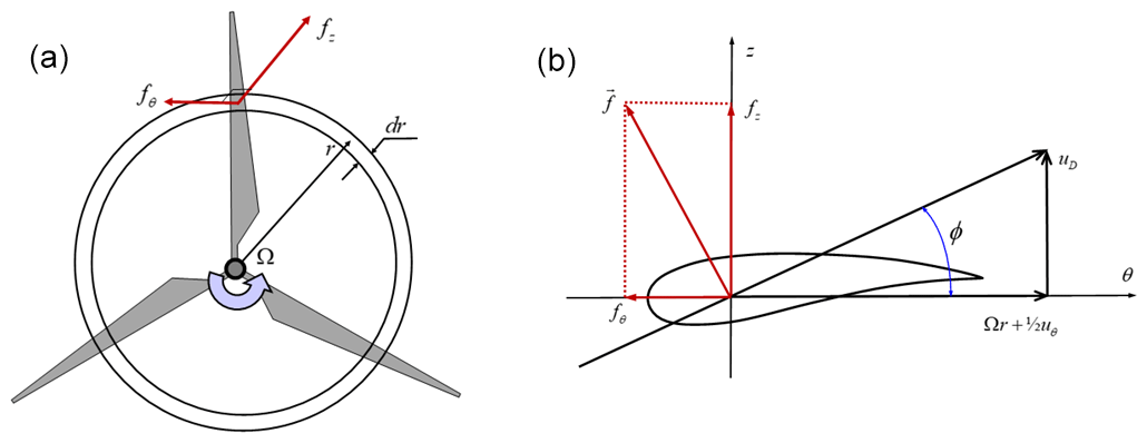
Figure 2 Geometry, kinematics, and forces acting on the rotor. (a) Forces acting in the rotor plane; (b) forces and velocity triangle on a cross section of the rotor.

In dimensionless form, the equations read

$$\begin{array}{}\text{(9a)}& {\displaystyle }& {\displaystyle \frac{f_z}{\mathrm{1}/\mathrm{2}\mathit{\rho }{U}_{\mathrm{0}}^{\mathrm{2}}}}={\displaystyle \frac{u_{\mathit{\theta }}}{U_{\mathrm{0}}}}\left(\mathrm{2}\mathit{\lambda }x+{\displaystyle \frac{u_{\mathit{\theta }}}{U_{\mathrm{0}}}}\right),\text{(9b)}& {\displaystyle }& {\displaystyle \frac{f_{\mathit{\theta }}}{\mathrm{1}/\mathrm{2}\mathit{\rho }{U}_{\mathrm{0}}^{\mathrm{2}}}}=\mathrm{2}{\displaystyle \frac{u_D}{U_{\mathrm{0}}}}{\displaystyle \frac{u_{\mathit{\theta }}}{U_{\mathrm{0}}}},\end{array}$$

where $x=r/R$ is the dimensionless radial position, and $\mathit{\lambda }=\mathrm{\Omega }R/U_{\mathrm{0}}$ is the tip-speed ratio.

The total axial force (thrust) and the power are determined by integration of the above equations,

$$\begin{array}{}\text{(10a)}& T=\underset{\mathrm{0}}{\overset{R}{\int }}{f}_z\mathrm{2}\mathit{\pi }r\mathrm{d}r=\mathrm{2}\mathit{\pi }\mathit{\rho }\underset{\mathrm{0}}{\overset{R}{\int }}r{u}_{\mathit{\theta }}\left(\mathrm{\Omega }r+\mathrm{1}/\mathrm{2}{u}_{\mathit{\theta }}\right)\mathrm{d}r,\end{array}$$

and

$$\begin{array}{}\text{(10b)}& P=\mathrm{\Omega }\underset{\mathrm{0}}{\overset{R}{\int }}r{f}_{\mathit{\theta }}\mathrm{2}\mathit{\pi }r\mathrm{d}r=\mathrm{2}\mathit{\pi }\mathit{\rho }\mathrm{\Omega }{u}_D\underset{\mathrm{0}}{\overset{R}{\int }}{u}_{\mathit{\theta }}{r}^{\mathrm{2}}\mathrm{d}r,\end{array}$$

which in dimensionless form reads

$$\begin{array}{}\text{(11a)}& {\displaystyle }& {\displaystyle }{C}_{\mathrm{T}}={\displaystyle \frac{T}{\mathrm{1}/\mathrm{2}\mathit{\rho }\mathit{\pi }{R}^{\mathrm{2}}{U}_{\mathrm{0}}^{\mathrm{2}}}}=\mathrm{4}\mathit{\lambda }\underset{\mathrm{0}}{\overset{\mathrm{1}}{\int }}{\displaystyle \frac{u_{\mathit{\theta }}}{U_{\mathrm{0}}}}{x}^{\mathrm{2}}\mathrm{d}x+\mathrm{2}\underset{\mathrm{0}}{\overset{\mathrm{1}}{\int }}{\left({\displaystyle \frac{u_{\mathit{\theta }}}{U_{\mathrm{0}}}}\right)}^{\mathrm{2}}x\mathrm{d}x,\text{(11b)}& {\displaystyle }& {\displaystyle }{C}_{\mathrm{P}}={\displaystyle \frac{P}{\mathrm{1}/\mathrm{2}\mathit{\rho }\mathit{\pi }{R}^{\mathrm{2}}{U}_{\mathrm{0}}^{\mathrm{3}}}}=\mathrm{4}\mathit{\lambda }\underset{\mathrm{0}}{\overset{\mathrm{1}}{\int }}{\displaystyle \frac{u_D}{U_{\mathrm{0}}}}{\displaystyle \frac{u_{\mathit{\theta }}}{U_{\mathrm{0}}}}{x}^{\mathrm{2}}\mathrm{d}x.\end{array}$$

From the above relations it is seen that a closure of the equations only demands knowledge about the azimuthal velocity distribution immediately behind the turbine.

For a wind turbine operating below the rated wind speed, it is assumed that the rotor loading corresponds to the one obtained for an optimum rotor. Although the design of modern wind turbine rotors is based on different design objectives and constraints, the actual geometry generally does not vary much. This assumption is supported by previous analyses by comparing optimum blade geometries generated using different rotor models. In Sørensen (2016) and Sørensen et al. (2021), a comparative study showed that, for tip-speed ratios typically used for the design of modern wind turbines, the different design methodologies approximately resulted in the same blade geometries. The idea behind the analytical model developed by Sørensen et al. (2019) is that an optimally designed blade is achieved by representing the rotor load by a constant circulation, modified with a tip correction, F(r), and a root correction, g(r). However, when operating a turbine at wind speeds higher than the rated one, it becomes necessary to reduce the loading by regulating the pitch setting in order to maintain a constant power output. The impact of this is a redistribution of the loading, which no longer can be represented by a constant circulation. Since the difference in loading from the optimum one will create additional losses in the wake, the azimuthal velocity distribution forming the loading in Eqs. (9a) and (9b) needs to include terms taking this into account. In the proposed model, the azimuthal velocity distribution not only is represented by the induction from root and tip vortices but also includes a term corresponding to a solid-body rotation of the wake. When pitching the rotor, this term will be active and ensure that the model includes the wake losses generated by the pitch setting. Hence, in the new extended model, the azimuthal velocity distribution is given as

$$\begin{array}{}\text{(12)}& {\displaystyle \frac{u_{\mathit{\theta }}}{U_{\mathrm{0}}}}=\left[{\displaystyle \frac{q_{\mathrm{0}}}{x}}-S_{\mathrm{0}}x\right]g\left(x\right)F\left(x\right),\end{array}$$

where the first term in the bracket corresponds to the optimum constant circulation condition, and the next term defines the redistribution of circulation due to the change in pitch setting when operating at wind speeds higher than the rated. The quantities q₀ and S₀ are constants representing the circulation of the optimum rotor and the rotation of the solid-body term, respectively. It should be emphasized that the used formula consists of a combination of a potential vortex, $u_{\mathit{\theta }}=C_{\mathrm{1}}/x$, and a solid-body rotation, u_θ=C₂x, which are both fundamental solutions to the steady incompressible Euler and Navier–Stokes equations in the case of a parallel flow. As tip correction we employ the model proposed by Glauert (1935):

$$\begin{array}{}\text{(13)}& F={\displaystyle \frac{\mathrm{2}}{\mathit{\pi }}}\arccos \left[\exp \left(-{\displaystyle \frac{N_{\mathrm{b}}(\mathrm{1}-x)}{\mathrm{2}\sin \mathit{\varphi }}}\right)\right],\end{array}$$

where N_b denotes the number of rotor blades and ϕ is the local flow angle, which approximately can be determined from the formula

$$\begin{array}{}\text{(14)}& \sin \mathit{\varphi }={\displaystyle \frac{\mathrm{1}}{\sqrt{\mathrm{1}+{\mathit{\lambda }}^{\mathrm{2}}{x}^{\mathrm{2}}/{\left(\frac{u_D}{U_{\mathrm{0}}}\right)}^{\mathrm{2}}}}}.\end{array}$$

It should be mentioned that we in the original work (Sørensen et al., 2019) used the tip correction of Prandtl. However, to be consistent with usual standards in blade element momentum (BEM) theory, this is replaced by the tip correction of Glauert. To account for the influence of the hub and the inner non-lifting part of the rotor, a vortex core of size δ is introduced, and an expression for the root correction is proposed as follows:

$$\begin{array}{}\text{(15)}& g=\mathrm{1}-\exp \left[-a{\left({\displaystyle \frac{x}{\stackrel{\mathrm{‾}}{\mathit{\delta }}}}\right)}^b\right],\end{array}$$

where $\stackrel{\mathrm{‾}}{\mathit{\delta }}=\frac{\mathit{\delta }}{R}$ denotes the dimensionless radial distance to the point where the maximum azimuthal velocity is achieved. With the proposed model, $\stackrel{\mathrm{‾}}{\mathit{\delta }}$ typically corresponds to the point where the lifting surface of the rotor starts. In the general case, the relation between the constants a and b is determined by differentiating Eq. (15) to determine the maximum azimuthal velocity at $x=\stackrel{\mathrm{‾}}{\mathit{\delta }}$. Here, we assume g to be represented by a fourth-order polynomial; hence, we get the values b=4 and a=2.335. A derivation of the general relationship between a and b is given in Appendix A.

Inserting Eq. (12) into Eqs. (9a) and (9b), the following expressions are obtained:

$$\begin{array}{}\text{(16a)}& {\displaystyle }\begin{array}{rl}{\displaystyle \frac{f_z}{\mathrm{1}/\mathrm{2}\mathit{\rho }{U}_{\mathrm{0}}^{\mathrm{2}}}}=& \left(\mathrm{2}\mathit{\lambda }x+\left({\displaystyle \frac{q_{\mathrm{0}}}{x}}-S_{\mathrm{0}}x\right)g\left(x\right)F\left(x\right)\right)\\ & \left[{\displaystyle \frac{q_{\mathrm{0}}}{x}}-S_{\mathrm{0}}x\right]g\left(x\right)F\left(x\right),\end{array}\text{(16b)}& {\displaystyle }\begin{array}{rl}& {\displaystyle \frac{f_{\mathit{\theta }}}{\mathrm{1}/\mathrm{2}\mathit{\rho }{U}_{\mathrm{0}}^{\mathrm{2}}}}=\mathrm{2}{\displaystyle \frac{u_D}{U_{\mathrm{0}}}}\left[{\displaystyle \frac{q_{\mathrm{0}}}{x}}-S_{\mathrm{0}}x\right]g\left(x\right)F\left(x\right).\end{array}\end{array}$$

Inserting Eq. (12) into Eq. (11a), we get

$$\begin{array}{}\text{(17)}& \begin{array}{rl}{C}_{\mathrm{T}}=& \underset{\mathrm{0}}{\overset{\mathrm{1}}{\int }}\mathrm{2}x\left(\mathrm{2}\mathit{\lambda }x+\left({\displaystyle \frac{q_{\mathrm{0}}}{x}}-S_{\mathrm{0}}x\right)g\left(x\right)F\left(x\right)\right)\\ & \left[{\displaystyle \frac{q_{\mathrm{0}}}{x}}-S_{\mathrm{0}}x\right]g\left(x\right)F\left(x\right)\mathrm{d}x\Rightarrow C_{\mathrm{T}}=\mathrm{2}{a}_{\mathrm{1}}{q}_{\mathrm{0}}^{\mathrm{2}}\\ & +\mathrm{4}{a}_{\mathrm{2}}\mathit{\lambda }{q}_{\mathrm{0}}-\mathrm{4}{a}_{\mathrm{3}}{S}_{\mathrm{0}}{q}_{\mathrm{0}}-\mathrm{4}{a}_{\mathrm{4}}\mathit{\lambda }{S}_{\mathrm{0}}+\mathrm{2}{a}_{\mathrm{5}}{S}_{\mathrm{0}}^{\mathrm{2}}.\end{array}\end{array}$$

The coefficients from the integration are given as follows:

$$\begin{array}{ll}{\displaystyle }& {\displaystyle }{a}_{\mathrm{1}}=\underset{\mathrm{0}}{\overset{\mathrm{1}}{\int }}{\displaystyle \frac{g^{\mathrm{2}}{F}^{\mathrm{2}}}{x}}\mathrm{d}x;a_{\mathrm{2}}=\underset{\mathrm{0}}{\overset{\mathrm{1}}{\int }}gFx\mathrm{d}x,\\ {\displaystyle }& {\displaystyle }{a}_{\mathrm{3}}=\underset{\mathrm{0}}{\overset{\mathrm{1}}{\int }}{g}^{\mathrm{2}}{F}^{\mathrm{2}}x\mathrm{d}x;a_{\mathrm{4}}=\underset{\mathrm{0}}{\overset{\mathrm{1}}{\int }}gF{x}^{\mathrm{3}}\mathrm{d}x,\\ {\displaystyle }& {\displaystyle }{a}_{\mathrm{5}}=\underset{\mathrm{0}}{\overset{\mathrm{1}}{\int }}{g}^{\mathrm{2}}{F}^{\mathrm{2}}{x}^{\mathrm{3}}\mathrm{d}x.\end{array}$$

From Eq. (17), the dimensionless reference circulation is determined as

$$\begin{array}{}\text{(18)}& \begin{array}{rl}& q_{\mathrm{0}}=\\ & {\displaystyle \frac{\sqrt{{\left(a_{\mathrm{2}}\mathit{\lambda }-a_{\mathrm{3}}{S}_{\mathrm{0}}\right)}^{\mathrm{2}}+a_{\mathrm{1}}\left(\mathrm{1}/\mathrm{2}{C}_{\mathrm{T}}+\mathrm{2}{a}_{\mathrm{4}}\mathit{\lambda }{S}_{\mathrm{0}}-a_{\mathrm{5}}{S}_{\mathrm{0}}^{\mathrm{2}}\right)}-\left(a_{\mathrm{2}}\mathit{\lambda }-a_{\mathrm{3}}{S}_{\mathrm{0}}\right)}{a_{\mathrm{1}}}}.\end{array}\end{array}$$

Inserting Eq. (12) into Eq. (11b), we get

$$\begin{array}{}\text{(19)}& \begin{array}{rl}& C_{\mathrm{P}}=\mathrm{4}\mathit{\lambda }\underset{\mathrm{0}}{\overset{\mathrm{1}}{\int }}{x}^{\mathrm{2}}{\displaystyle \frac{u_D}{U_{\mathrm{0}}}}\left[{\displaystyle \frac{q_{\mathrm{0}}}{x}}-S_{\mathrm{0}}x\right]g\left(x\right)F\left(x\right)\mathrm{d}x\Rightarrow \\ & C_{\mathrm{P}}=\mathrm{4}\mathit{\lambda }\left(a_{\mathrm{6}}{q}_{\mathrm{0}}-a_{\mathrm{7}}{S}_{\mathrm{0}}\right),\end{array}\end{array}$$

where $a_{\mathrm{6}}=\underset{\mathrm{0}}{\overset{\mathrm{1}}{\int }}\frac{u_D}{U_{\mathrm{0}}}gFx\mathrm{d}x$, and $a_{\mathrm{7}}=\underset{\mathrm{0}}{\overset{\mathrm{1}}{\int }}\frac{u_D}{U_{\mathrm{0}}}gF{x}^{\mathrm{3}}\mathrm{d}x$.

It is seen that, keeping the axial velocity inside the integration, Eq. (19) allows for solutions involving non-constant inflow u_D=u_D(x). In Sørensen et al. (2019) it was demonstrated how arbitrary inflow velocity distributions can be included to determine local load distributions. However, in the present work, where the focus is on validating the basic approach, we assume a constant inflow. In this case, we get

$$\begin{array}{}\text{(20)}& C_{\mathrm{P}}=\mathrm{4}\mathit{\lambda }{\displaystyle \frac{u_D}{U_{\mathrm{0}}}}\left(a_{\mathrm{2}}{q}_{\mathrm{0}}-a_{\mathrm{4}}{S}_{\mathrm{0}}\right).\end{array}$$

Knowing the power coefficient, the axial velocity in the rotor plane is given as

$$\begin{array}{}\text{(21)}& \left({\displaystyle \frac{u_D}{U_{\mathrm{0}}}}\right)={\displaystyle \frac{C_{\mathrm{P}}}{\mathrm{4}\mathit{\lambda }\left(a_{\mathrm{2}}{q}_{\mathrm{0}}-a_{\mathrm{4}}{S}_{\mathrm{0}}\right)}}.\end{array}$$

The above-described system of equations forms the basis of the proposed analytical load model. Input to the model is (λ, C_T, C_P) or, alternatively, (λ, C_T, $u_D/U_{\mathrm{0}}$), depending on the aim of the analysis.

At wind speeds below the rated, the rotor is operated at a constant tip-speed ratio; hence, S₀=0 and the reference circulation is only a function of the rated tip-speed ratio, thrust coefficient, and power coefficient, $q_{\mathrm{0},\mathrm{r}}=q_{\mathrm{0}}({\mathit{\lambda }}_{\mathrm{r}},C_{\mathrm{T},\mathrm{r}},C_{\mathrm{P},\mathrm{r}})$. From Eq. (18), we get

$$\begin{array}{}\text{(22)}& q_{\mathrm{0},\mathrm{r}}={\displaystyle \frac{\sqrt{{\mathit{\lambda }}_{\mathrm{r}}^{\mathrm{2}}{a}_{\mathrm{2}}^{\mathrm{2}}+\mathrm{1}/\mathrm{2}{a}_{\mathrm{1}}{C}_{\mathrm{T},\mathrm{r}}}-{\mathit{\lambda }}_{\mathrm{r}}{a}_{\mathrm{2}}}{a_{\mathrm{1}}}},\end{array}$$

with the axial flow in the rotor plane computed from

$$\begin{array}{}\text{(23)}& {\left({\displaystyle \frac{u_D}{U_{\mathrm{0}}}}\right)}_{\mathrm{r}}={\displaystyle \frac{C_{\mathrm{P},\mathrm{r}}}{\mathrm{4}{\mathit{\lambda }}_{\mathrm{r}}{a}_{\mathrm{2}}{q}_{\mathrm{0},\mathrm{r}}}}.\end{array}$$

Hence, setting S₀=0, the dimensionless loading can be obtained directly as in the original analytical model derived by Sørensen et al. (2019). In Sørensen and Andersen (2020) this approach was shown to give excellent results for rotors operating at rated conditions. However, at operating conditions far from the rated, the assumption of a constant circulation supplemented with tip and root corrections was found not to be sufficient, and an extended modelling, as the one proposed here (Eq. 12), is required. In this context, two main questions remain to be answered. First, does the proposed extended model, Eqs. (16a) and (16b), actually represent the loads on a real rotor operating at off-design conditions? Secondly, since an additional parameter, S₀, is introduced, an additional relationship connecting this parameter and the existing input parameters is required in order to establish a solution at off design. How do we model this? These two questions will be addressed in the following section.

3 Verification and tuning of model

In this section, we verify the basic behaviour of the proposed load model and tune the modelling parameter S₀.

3.1 Verification of the model at off-design conditions

A simple way to verify the applicability of the proposed model to represent the loadings at off-design conditions is to compare it to results obtained from blade element momentum (BEM) computations of an actual wind turbine. Since the parameter, S₀, is not known, we simply try different values and chose the one that gives the best fit of the analytical load distributions to those computed by the BEM technique. As a reference, we chose the geometry of the NEG Micon NM80 wind turbine, which in the previous study by Sørensen and Andersen (2020) was employed to test the model for S₀=0 (more details about the NM80 turbine are given in Appendix B). Here, we chose three different operating conditions, one corresponding to the rated condition (C_T=0.82) and two off-design conditions (C_T=0.26 and C_T=0.13).

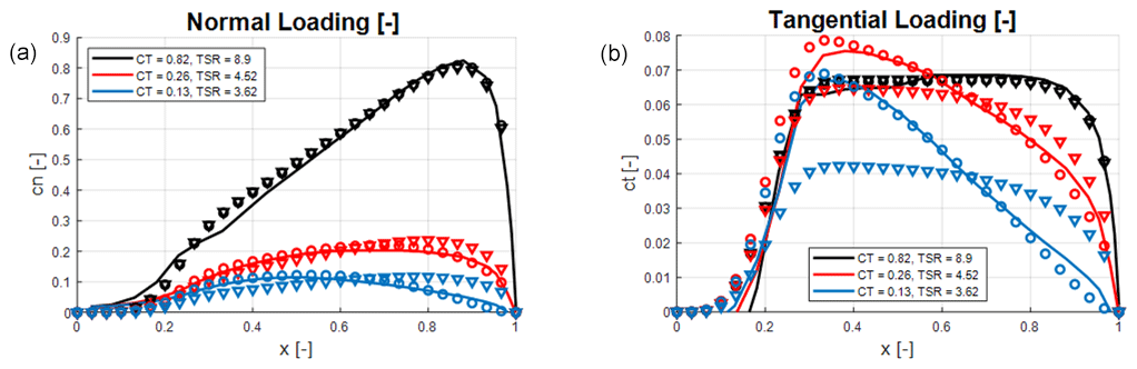
Figure 3 Comparison between analytical model and BEM computations. Solid lines: BEM computations, triangles: analytical model assuming S₀=0, and circles: analytical model using “optimized” S₀ values. (a) Normal load distributions; (b) tangential load distributions.

In the following we compare dimensionless normal and tangential load distributions along a blade. The distributions are normalized by $\mathit{\rho }R{U}_{\mathrm{0}}^{\mathrm{2}}$; hence, the dimensionless quantities are given as

$$\begin{array}{}\text{(24)}& C_{\mathrm{n}}={\displaystyle \frac{F_{\mathrm{n}}[N/m]}{\mathit{\rho }R{U}_{\mathrm{0}}^{\mathrm{2}}}};C_{\mathrm{t}}={\displaystyle \frac{F_{\mathrm{t}}[N/m]}{\mathit{\rho }R{U}_{\mathrm{0}}^{\mathrm{2}}}},\end{array}$$

where F_n is the normal loading and F_t is the tangential loading on each blade. As the analytical loads in Eqs. (9a) and (9b) are given per area unit for the full rotor, the load coefficients are computed as

$$\begin{array}{}\text{(25)}& C_{\mathrm{n}}=\left({\displaystyle \frac{f_z}{\mathrm{1}/\mathrm{2}\mathit{\rho }{U}_{\mathrm{0}}^{\mathrm{2}}}}\right)\cdot \left({\displaystyle \frac{\mathit{\pi }x}{N_{\mathrm{b}}}}\right);C_{\mathrm{t}}=\left({\displaystyle \frac{f_{\mathit{\theta }}}{\mathrm{1}/\mathrm{2}\mathit{\rho }{U}_{\mathrm{0}}^{\mathrm{2}}}}\right)\cdot \left({\displaystyle \frac{\mathit{\pi }x}{N_{\mathrm{b}}}}\right),\end{array}$$

where N_b denotes the number of blades.

The results are shown in Fig. 3, which depicts distributions of normal loadings (left) and tangential loadings (right). In the plots, the BEM computations are given as solid lines, and the analytical results are given symbols (a triangle for S₀=0 and a circle for the “optimum” S₀ value). First, it is observed that the comparison between BEM and the analytical model at rated conditions (black curves) displays an excellent agreement. Here, the optimum S₀ value is zero, confirming that the original model actually is working well for the case at which it is developed. In the two off-design cases, on the other hand, it is clearly seen that it is required to extend the model with an additional term. In particular, the tangential loading becomes way off if we maintain a value of S₀=0, where the distributions tends to keep a nearly constant tangential load distribution over the main part of the rotor blade. Since we have no expression to determine S₀, we try different values and choose the one that gives the distributions most close to the BEM computations. In Appendix C, assuming that the blade in the extreme case locally near the tip will start to operate as a propeller, it was possible to derive a simple relation for the maximum value of S₀, stating that S₀<0.08. In the present case, by trial and error, the values are found to be S₀=0.019 for C_T=0.26 and S₀=0.044 for C_T=0.13. Employing these values, the comparison displays an excellent agreement for both the normal and tangential load distributions, demonstrating that the proposed model actually takes into account the main features of the load distributions at off-design conditions. However, it is still needed to develop a general expression for the rotation parameter S₀.

3.2 Modelling of the rotation parameter S₀

To determine an expression for the rotation parameter S₀, we first recognize that S₀ is equal to zero for a rotor operating at rated conditions. Hence, it is natural to seek for an expression that depends on how far the rotor is operating from the rated one, i.e. search for a relationship $S_{\mathrm{0}}=S_{\mathrm{0}}({\mathit{\lambda }}_{\mathrm{r}}-\mathit{\lambda })$ or $S_{\mathrm{0}}=S_{\mathrm{0}}(C_{\mathrm{T},\mathrm{r}}-C_{\mathrm{T}})$, where λ_r and C_T,r denote the rated values of the tip-speed ratio and the thrust coefficient, respectively. To accomplish this, as a starting point we carry out a series of BEM computations for actual wind turbines operating at different conditions. The used wind turbines are the Vestas V27 and V52 turbines and the NEG Micon NM80 turbine. The relevant data for the turbines are given in Appendix B. The computations are carried out at different operating conditions, and the outcome is employed to determine if there exists a simple parameterizable relationship between S₀ and the input variables. Hence, for each combination of λ and C_T, a BEM computation of the normal and tangential loading distributions is carried out, and the value of S₀ that best fits the distributions with the analytical model is determined. The outcome of this is for the three wind turbines and different combinations of tip-speed ratio and thrust coefficients shown in Fig. 4, where S₀ is plotted as a function of normalized values of the tip-speed ratio, $({\mathit{\lambda }}_{\mathrm{r}}-\mathit{\lambda })/{\mathit{\lambda }}_{\mathrm{r}}$, and thrust coefficient, $(C_{\mathrm{T},\mathrm{r}}-C_{\mathrm{T}})/C_{\mathrm{T},\mathrm{r}}$. Analysing the two distributions, it is seen that using the normalized tip-speed ratio to determine S₀ results in some scatter of the data, whereas there is a more unique relationship between S₀ and the normalized thrust coefficient.

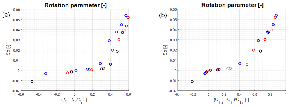
Figure 4 Correlation between rotation parameter, S₀, and dimensionless relative tip-speed ratio (a) and thrust coefficient (b). Red circles: V27, blue circles: V52, and black circles: NM80.

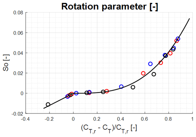
Figure 5 Curve fit given the parameterization of S₀ with respect to the normalized thrust coefficient. Red circles: V27, blue circles: V52, and black circles: NM80.

Employing a simple least squares fit using the relationship

$$\begin{array}{}\text{(26)}& S_{\mathrm{0}}=\mathit{\alpha }{\left({\displaystyle \frac{C_{\mathrm{T},\mathrm{r}}-C_{\mathrm{T}}}{C_{\mathrm{T},\mathrm{r}}}}\right)}^{\mathit{\beta }},\end{array}$$

we get the values α=0.08 and β=3 for $C_{\mathrm{T}}<C_{\mathrm{T},\mathrm{r}}$ and α=0.05 and β=1 for $C_{\mathrm{T}}\ge C_{\mathrm{T},\mathrm{r}}$. The result of the fit is shown in Fig. 5, which displays a very good agreement between the computed points and the curve fit. Hence, the closure of the equations is accomplished by exploiting the below expression to connect the rotation parameter S₀ with the normalized thrust coefficient:

$$\begin{array}{}\text{(27)}& S_{\mathrm{0}}=\left\{\begin{array}{ll}\mathrm{0.08}\cdot {\left(\frac{C_{\mathrm{T},\mathrm{r}}-C_{\mathrm{T}}}{C_{\mathrm{T},\mathrm{r}}}\right)}^{\mathrm{3}};& C_{\mathrm{T}}<C_{\mathrm{T},\mathrm{r}}\\ \mathrm{0.05}\cdot \left(\frac{C_{\mathrm{T},\mathrm{r}}-C_{\mathrm{T}}}{C_{\mathrm{T},\mathrm{r}}}\right);& C_{\mathrm{T}}\ge C_{\mathrm{T},\mathrm{r}}\end{array}\right..\end{array}$$

As a conclusion of the parameterization, we now have a closure of S₀ at off-design conditions that, besides the actual thrust coefficient, C_T, also demands knowledge about the rated thrust coefficient, C_T,r. For an actual wind turbine, this value is normally given as a part of the general technical data. If this is not known, a value of 0.8, which is typical for a commercial wind turbine, may be employed.

4 Results

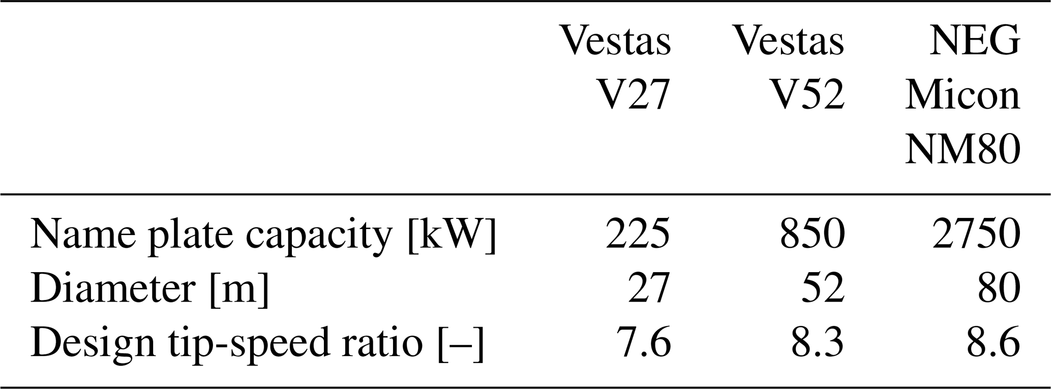
In the following we show various comparative results for three different wind turbines operating at a broad range of conditions. The BEM computations are carried out using full knowledge regarding the actual blade geometry and associated airfoil data. The operational conditions contain all kinds of combinations between the tip-speed ratio and the thrust coefficient, including high wind speeds, corresponding with low thrust coefficients. In this case, the thrust coefficient is lowered by pitching the rotor blades. In contrast with the detailed input required in the BEM computations, the analytic model only demands tip-speed ratio, thrust coefficient, and power coefficient as input. The computations are carried out for a constant axial inflow without shear and turbulence. As demonstrated in Sørensen et al. (2019), shear and turbulence are easily introduced into the model when carrying out actual CFD actuator disc computations, but it is not the objective of the present work to include this. Here we focus on assessing the models ability to represent loadings for different turbines operating at off-design conditions. The chosen wind turbines represent sizes with a range of nameplate capacity from 225 to 2750 kW. The data for the wind turbines are given below in Appendix B, which shows nameplate capacity, rotor diameter, and design tip-speed ratio. The latter information is included to assess where the best agreement between the analytical model and the BEM computations can be expected to take place.

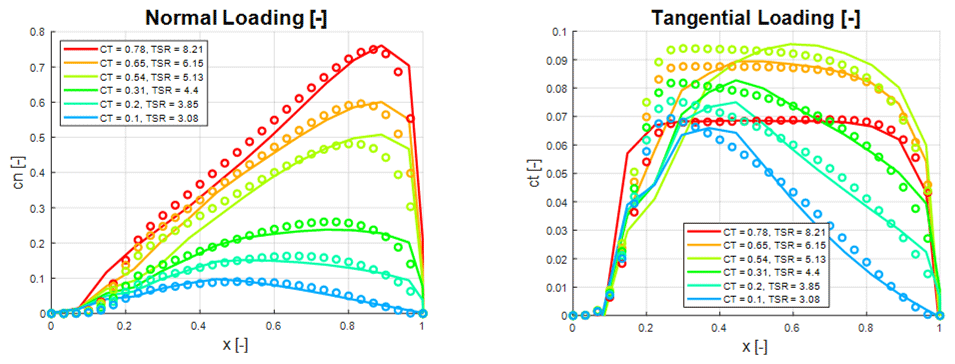
Figure 6 Normal and tangential force coefficient distribution of the V27 turbine at different tip-speed ratios and thrust coefficients. Circles: analytical model; solid lines: BEM computations.

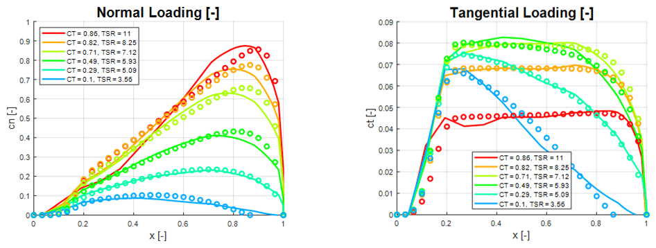
Figure 7 Normal and tangential force coefficient distribution of the V52 turbine at different tip-speed ratios and thrust coefficients. Circles: analytical model; solid lines: BEM computations.

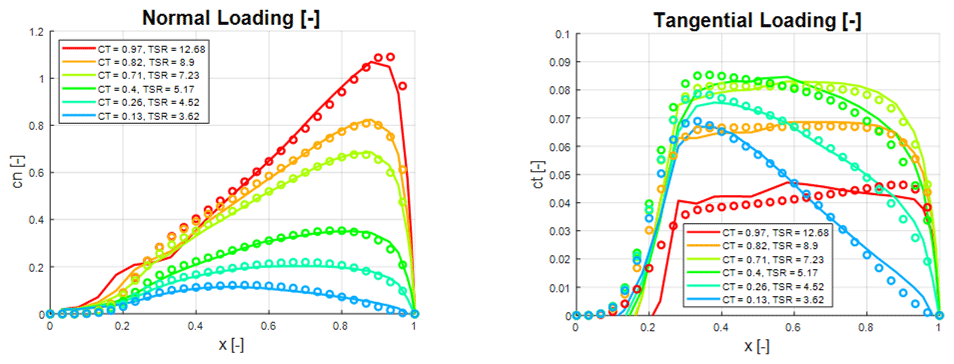
Figure 8 Normal and tangential force coefficient distribution of the NM80 turbine at different tip-speed ratios and thrust coefficients. Circles: analytical model; solid lines: BEM computations.

In Figs. 6–8 the load distributions are compared for three wind turbines operating at a wide range of off-design conditions, with thrust coefficients ranging from 0.1 to 0.97 and tip-speed ratios between 3 and 13, where the turbine is either pitch regulated or running at upstart conditions. The only input to the analytical model is the tip-speed ratio, λ, and the C_T and C_P values from the BEM computations. Figure 6 shows comparative normal and tangential force distributions for the V27 rotor. As seen, there is a generally a very good agreement between the analytical and the BEM-computed normal force distributions. The agreement between analytical and computed tangential force coefficients is good over most of the rotor surface but not as convincing as for the normal force distributions. The biggest deviation between computed and analytical tangential loadings is seen to appear at the inner part of the blade for moderate C_T values, whereas the best comparisons are obtained for high and low C_T values. Figure 7 compares computed and analytical force coefficients for the V52 wind turbine. As compared to the V27 data, we here observe an even better agreement between analytical and computed force distributions. In particular, the comparison between the analytical representation of the tangential force distribution and the computed one is excellent for all the predicted cases. However, some deviation is observed for the normal force coefficients at the outer part of the blade. The best comparison between the analytical and the computed force coefficients is found for the NM80 turbine, as shown in Fig. 8. Here we observe an excellent agreement between the analytical and numerical curves for all C_T values.

5 Discussion

The comparisons between the BEM computations and the analytical load distributions are generally in very good agreement with each other, even for wind turbines operating far away from the rated design-based conditions. This actually supports the underlying hypothesis that there exists a general way of describing the loading on a wind turbine using a simple analytical expression with only very few input parameters. For the present investigation, input parameters are the thrust and power coefficients as function of tip-speed ratio. In a large-eddy simulation of, for example, a wind farm, the velocity distribution on the actuator disc (i.e. the rotor) is an inherent part of the simulation, and the unknown in this case is the generated power (see, for example, Nilsson et al., 2014, or van der Laan et al., 2015). There may be other ways of representing and generalizing the expressions for the loadings. The one proposed here, using circulation and rotation of the wake flow as a guideline to parameterize the loads, seems actually to work quite well. One may argue that using the BEM technique, which normally is characterized as a low-fidelity approach, as the basis for determining the missing relationship between the S₀ parameter and the thrust coefficient is not accurate enough. An answer to this is partly that the BEM technique, even today, is the only design tool used in industry for designing wind turbine rotors and partly that the methodology presented here is general, and the parameterization and tuning of the model easily can be improved later using more sophisticated prediction tools.

6 Conclusion

A generalized analytical body force model has been developed and validated against load distributions generated by a BEM model. The model, which is an extension of an earlier model that was only valid for optimum operating rotors, now includes load expressions for wind turbine rotors operating at off-design conditions. The essential part of the model is based on combining an expression for constant circulation with a solid-body rotation approach to take into account losses when operating the rotor at off-design conditions. A comparison with BEM computations was carried out using three wind turbines of different sizes running at a range of different operating conditions. The results are very convincing, showing generally a very good agreement between the simple analytical model and the BEM results. The comparison demonstrates that a simple analytical model with very good precision can be utilized to represent the loading on wind turbines, at both design and off-design conditions.

Appendix A

The expression for the root correction is derived from the idea that the inner part of the rotor is a viscous correction to the potential vortex forming the lift-producing part of loading. At design conditions (where S₀=0), the azimuthal velocity distribution near the root is given as

$$\begin{array}{}\text{(A1)}& {\displaystyle \frac{u_{\mathit{\theta }}}{U_{\mathrm{0}}}}={\displaystyle \frac{q_{\mathrm{0}}}{x}}\left[\mathrm{1}-\exp \left[-a{\left({\displaystyle \frac{x}{\stackrel{\mathrm{‾}}{\mathit{\delta }}}}\right)}^b\right]\right],\end{array}$$

where we implicitly assume that F=1. To determine the relationship between the constants a and b, we assume that the azimuthal velocity attains its maximum at the radial position, where $x=\stackrel{\mathrm{‾}}{\mathit{\delta }}$. Hence, the relation between a and b is determined by differentiating Eq. (A1) with respect to x and setting this expression equal to zero at $x=\stackrel{\mathrm{‾}}{\mathit{\delta }}$. Differentiating Eq. (A1) with respect to x gives

$$\begin{array}{}\text{(A2)}& \begin{array}{rl}{\displaystyle \frac{\mathrm{d}}{\mathrm{d}x}}\left({\displaystyle \frac{u_{\mathit{\theta }}}{U_{\mathrm{0}}}}\right)& =-{\displaystyle \frac{q_{\mathrm{0}}}{x^{\mathrm{2}}}}\left[\mathrm{1}-\exp \left[-a{\left({\displaystyle \frac{x}{\stackrel{\mathrm{‾}}{\mathit{\delta }}}}\right)}^b\right]\right]\\ & +{\displaystyle \frac{q_{\mathrm{0}}}{x}}\exp \left[-a{\left({\displaystyle \frac{x}{\stackrel{\mathrm{‾}}{\mathit{\delta }}}}\right)}^b\right]{\displaystyle \frac{ab}{\stackrel{\mathrm{‾}}{\mathit{\delta }}}}{\left({\displaystyle \frac{x}{\stackrel{\mathrm{‾}}{\mathit{\delta }}}}\right)}^{b-\mathrm{1}}.\end{array}\end{array}$$

Inserting $x=\stackrel{\mathrm{‾}}{\mathit{\delta }}$ and setting the expression equal to zero gives the following relation between a and b:

$$\begin{array}{}\text{(A3)}& (a\cdot b+\mathrm{1})\exp (-a)=\mathrm{1}.\end{array}$$

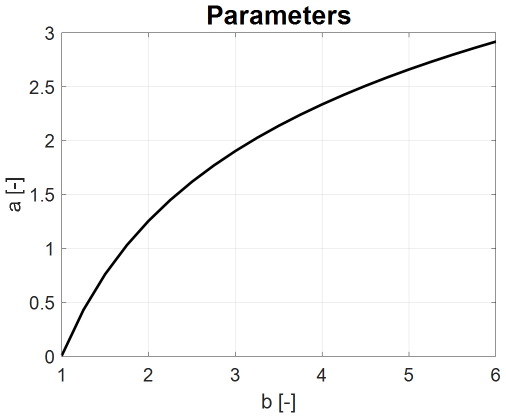
We observe here that the expression does not include the viscous core size, $\stackrel{\mathrm{‾}}{\mathit{\delta }}$, but is a generic expression for the relationship between the parameters a and b. Since the equation is non-linear, it is required to solve it numerically. Doing this, the relationship between a and b is as shown in Fig. A1. In the present work, we put b=4 and get that a=2.335.

Figure A1 Plot showing the relationship between the parameters a and b (Eq. A3).

Appendix B

Here we give the main characteristics of the turbines used in the study. We do not present detailed data, such as chord and twist distributions or the employed airfoil characteristics, as they are confidential. However, for the present study these data are not needed, since only the outcome of the BEM computations is required to develop and validate the developed model. Details of the Vestas V27 turbine can be found in Resor and LeBlanc (2014) and Kelley and White (2018), and for the V52 turbine, the reader is referred to the home page https://en.wind-turbine-models.com/turbines/71-vestas-v52 (last access: May 2023).

Table B1 Wind turbine characteristics.

Appendix C

Here we derive a simple guideline for determining an upper limit of the rotation constant S₀, which was introduced in Eq. (12) to take into account off-design operating conditions. First, as explained in Sect. 2.1, for wind speeds exceeding the rated, the off-design conditions are given by pitching the blades, keeping a constant or nearly constant tip speed. Hence, for increasing wind speeds the tip-speed ratio decreases, and by increasing the pitch angle the power production is maintained at a constant value, corresponding to the nameplate capacity of the turbine. Unfortunately, there is no simple way of relating this process to the determination of S₀. Instead, we resort to some simple physical considerations. First, assuming the tip-speed ratio to be larger than about three, with a very good approximation, Eq. (17) may be written as

$$\begin{array}{}\text{(C1)}& C_{\mathrm{T}}\simeq \mathrm{4}{a}_{\mathrm{2}}\mathit{\lambda }{q}_{\mathrm{0}}-\mathrm{4}{a}_{\mathrm{4}}\mathit{\lambda }{S}_{\mathrm{0}},\end{array}$$

from which we get

$$\begin{array}{}\text{(C2)}& q_{\mathrm{0}}\simeq \left({\displaystyle \frac{a_{\mathrm{4}}}{a_{\mathrm{2}}}}\right)S_{\mathrm{0}}+{\displaystyle \frac{C_{\mathrm{T}}}{\mathrm{4}{a}_{\mathrm{2}}\mathit{\lambda }}}.\end{array}$$

Next, if the rotor has to run locally in a turbine mode, i.e. if it everywhere along the blade extracts energy from the wind, the tangential force component, f_θ, has to be positive. However, at high wind speeds a pitch-regulated wind turbine rotor will locally, starting around the tip, begin to operate as a propeller, i.e. f_θ will become negative and start to deliver energy to the flow. Assuming now that the rotor somewhere near the tip starts to act locally as a propeller, from Eq. (16) we get that the term ($q_{\mathrm{0}}/x-S_{\mathrm{0}}x$) becomes negative. Assuming that this happens at a reference point x=x_p, we get

$$\begin{array}{}\text{(C3)}& q_{\mathrm{0}}\simeq S_{\mathrm{0}}{x}_{\mathrm{p}}^{\mathrm{2}}.\end{array}$$

Combining Eqs. (C2) and (C3), we get that

$$\begin{array}{}\text{(C4)}& S_{\mathrm{0}}\simeq {\displaystyle \frac{C_{\mathrm{T}}}{\mathrm{4}\mathit{\lambda }\left(a_{\mathrm{2}}{x}_{\mathrm{p}}^{\mathrm{2}}-a_{\mathrm{4}}\right)}}.\end{array}$$

With the approximate values a₂≃0.4 and a₄≃0.2, we get that

$$\begin{array}{}\text{(C5)}& S_{\mathrm{0}}\simeq \mathrm{1.25}{\displaystyle \frac{C_{\mathrm{T}}}{\mathit{\lambda }\left(\mathrm{2}{x}_{\mathrm{p}}^{\mathrm{2}}-\mathrm{1}\right)}},\end{array}$$

which serves as a simple guideline for the upper value of S₀. In the cases that have been run in the present study, the most extreme values were C_T=0.1 and λ=3.56, where the V52 rotor was found to go into a propeller mode at x_p=0.85, resulting in an upper limit $S_{\mathrm{0},\max }\simeq \mathrm{0.08}$.