the Creative Commons Attribution 4.0 License.
the Creative Commons Attribution 4.0 License.
 | 18 Jul 2023
Modelling the impact of trapped lee waves on offshore wind farm power output
Sarah J. Ollier
Simon J. Watson
Mesoscale meteorological phenomena, including atmospheric gravity waves (AGWs) and including trapped lee waves (TLWs), can result from flow over topography or coastal transition in the presence of stable atmospheric stratification, particularly with strong capping inversions. Satellite images show that topographically forced TLWs frequently occur around near-coastal offshore wind farms. Yet current understanding of how they interact with individual turbines and whole farm energy output is limited. This parametric study investigates the potential impact of TLWs on a UK near-coastal offshore wind farm, Westermost Rough (WMR), resulting from westerly–southwesterly flow over topography in the southeast of England.
Computational fluid dynamics (CFD) modelling (using Ansys CFX) of TLW situations based on real atmospheric conditions at WMR was used to better understand turbine level and whole wind farm performance in this parametric study based on real inflow conditions. These simulations indicated that TLWs have the potential to significantly alter the wind speeds experienced by and the resultant power output of individual turbines and the whole wind farm. The location of the wind farm in the TLW wave cycle was an important factor in determining the magnitude of TLW impacts, given the expected wavelength of the TLW. Where the TLW trough was coincident with the wind farm, the turbine wind speeds and power outputs were more substantially reduced compared with when the TLW peak was coincident with the location of the wind farm. These reductions were mediated by turbine wind speeds and wake losses being superimposed on the TLW. However, the same initial flow conditions interacting with topography under different atmospheric stability settings produce differing near-wind-farm flow. Factors influencing the flow within the wind farm under the different stability conditions include differing, hill and coastal transition recovery, wind farm blockage effects, and wake recovery. Determining how much of the differences in wind speed and power output in the wind farm resulted from the TLW is an area for future development.
- Article
(8511 KB) - Full-text XML
- BibTeX
- EndNote


Atmospheric gravity waves (AGWs) often result from displacement of flow by topographical obstacles in neutral or stable surface atmospheric conditions with a strong temperature inversion above the atmospheric boundary layer. They also form via jet stream turbulence, weather fronts, cold air outbreaks, thunderstorms, tornadoes, hurricanes, polar lows, and other unknown sources (Gossard and Hooke, 1975; Rasmussen and Aakjær, 1992; Romanova and Yakushkin, 1995; Chunchuzov et al., 2000; Nappo, 2012). The flow displaced by these conditions oscillates to create waves which modulate the local wind speed. AGWs are frequent in the offshore environment and influence marine atmospheric-boundary-layer wind fields over large areas of the ocean (e.g. Thomson et al., 1992; Vachon et al., 1994).
Strong stable capping temperature inversions aloft, often induced by changes in temperature at the coastal transition, provide a “lid” to trap the waves created by topographical obstacles, resulting in horizontally propagating AGWs, known as trapped lee waves (TLWs). In the last 12 years, AGW propagation instigated by wind farms themselves has been investigated (e.g. Smith, 2010; Allaerts and Meyers, 2017a, 2019, 2017b; Allaerts et al., 2018; Lanzilao and Meyers, 2021), and the impact of TLWs on onshore wind farms has recently been investigated (Xia et al., 2021; Draxl et al., 2021; Wilczak et al., 2019). However, to our knowledge, no one has investigated the influence of pre-existing TLWs on individual turbines or whole wind farms offshore, and computational fluid dynamics (CFD) investigations of TLW wind farm investigations have not been published. Considering their influence on offshore wind speeds, TLWs are likely to impact offshore wind power production. Thus, this research investigates the influence of TLWs on offshore wind farm power output using unsteady Reynolds-averaged Navier–Stokes (URANS) CFD simulations. Although this work focuses on resolving standing waves, a URANS solver was preferred for reasons of numerical stability. Influences on the flow under differing stability conditions are summarized in Fig. 1.
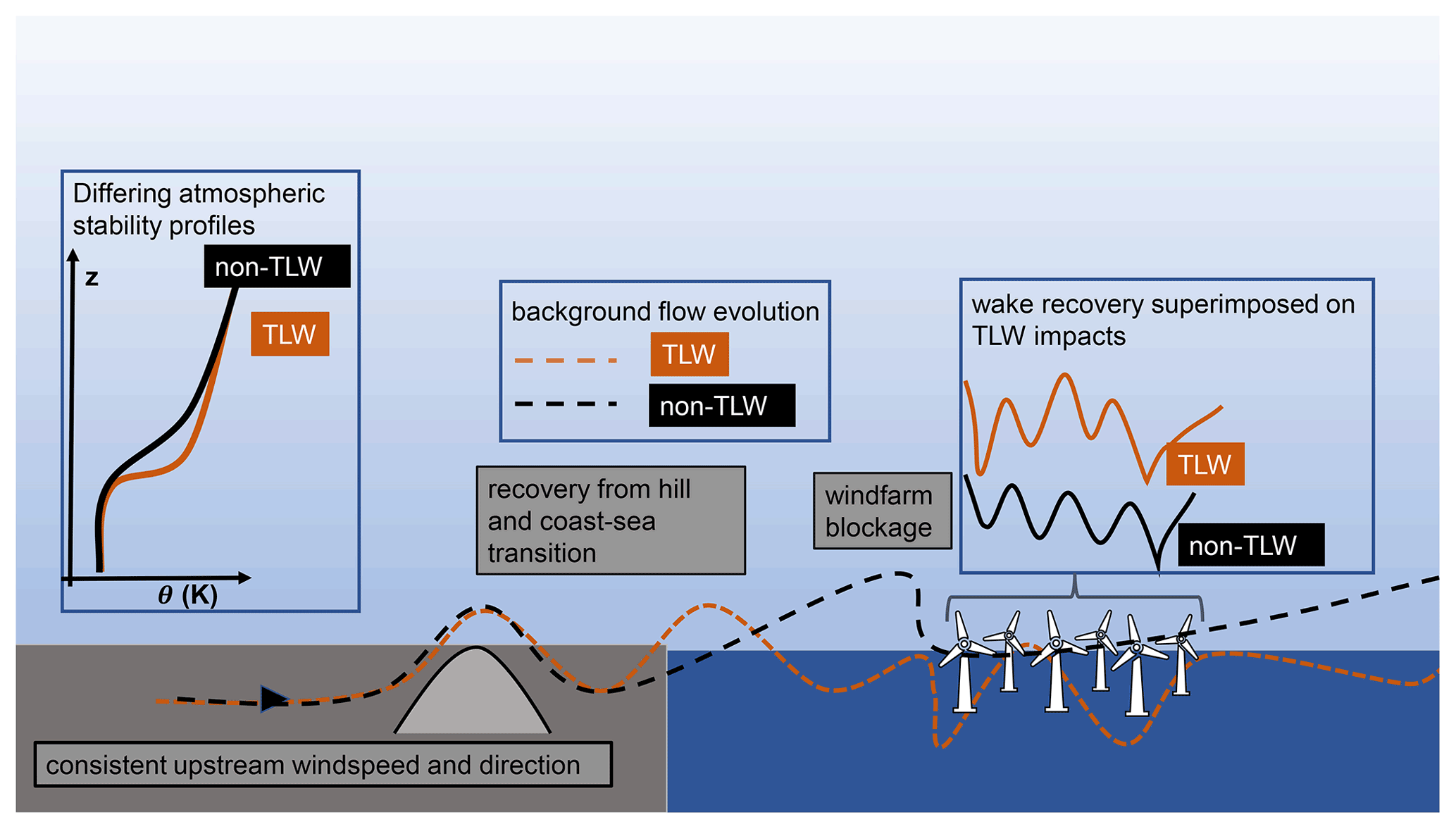
Figure 1Interaction of consistent wind speed and direction with different stability conditions upstream of a topographical obstacle and an offshore wind farm. The dashed lines show the evolution of flow aligned with a single column of wind turbines. This flow evolves under different stability conditions, a strong capping inversion for the TLW (orange), and a conventionally neutral boundary layer (CNBL, black) without TLWs (non-TLW). Insets show stability profiles (left) and wind farm wake recovery superimposed on the background flow for a single column of turbines aligned with the prevailing wind direction.
We use a theoretical offshore wind farm downstream of a topographical obstacle to simulate the impact of TLWs on the wind power output. Although the set-up is theoretical, the layout used is based in the operational offshore wind farm at Westermost Rough (WMR) off the East Yorkshire coast. This theoretical wind farm is referred to as WMR throughout this paper.
Wave damping
Erroneous wave reflection from the domain boundaries is a frequent problem in CFD models with AGWs. A solution to this problem is to introduce wave damping. Rayleigh damping, which absorbs waves before they can be reflected at domain boundaries, was first introduced in early, two-dimensional mountain wave models (Klemp and Lilly, 1978; Durran and Klemp, 1983) through the use of a simple damping term depending on the perturbation of a variable from its equilibrium value. This can be simplified to prognostic Eq. (1) (Warner, 2010).
Here, τ(z) is the Rayleigh damping coefficient, and α is a dependent variable, with the mean value of the dependent variable. Damping terms ξu, ξw, ξθ were added to the right-hand side of the equations in early work (Klemp and Lilly, 1978; Durran and Klemp, 1983). These were set to gradually increase in the upper half of the domain. In a recent large eddy simulation (LES) study (Allaerts and Meyers, 2017a), low wave reflection was also reported when there was space for at least one vertical wavelength, λz, beneath the damping layer (Allaerts and Meyers, 2017a), based on an earlier linear model (Klemp and Lilly, 1978), where λz is defined as
where U is the bulk wind speed and N is the freestream Brunt-Väisälä frequency (Eq. 3).
where g is gravitational acceleration in (ms−2), θ is potential temperature (K), and is the free atmosphere lapse rate. Whilst damping-layer strength, depth, location, and how the damping layers are implemented varies between studies, so do the atmospheric conditions (wind speed and inversion strength), domain dimensions, grid resolution, topography, wind farms sizes, and layouts. Thus, it is not possible to directly compare the methodologies and deduce the optimal conditions to transfer to other studies. Recent studies (Ollier et al., 2018; Jia et al., 2019) used RANS to model TLWs but do not detail their damping methodology. The literature discussed here uses LES configurations rather than RANS, some of which include a precursor domain (Gadde and Stevens, 2019; Wu and Porté-Agel, 2017), unlike the current work. Domain top Rayleigh damping strength ranged from 0.0001–0.016 s−1 in Allaerts and Meyers (2017a), Gadde and Stevens (2019), Haupt et al. (2019), and Hills and Durran (2012), with a range of upper-level damping thicknesses (1–16 km). A three-dimensional mountain ridge was included in Hills and Durran (2012), and no wind farm was included. A damping layer of 16 km in the vertical, from z=20 km to the domain extent (z=36 km), was used in a very large domain (1200 km × 1200 km × 36 km); no inflow or outflow damping was included. TLW reflection was observed, with stronger domain top damping in Hills and Durran (2012). The maximum damping in this layer was 0.005 s−1, gradually increasing from 0 s−1 outside the layer.
Damping near domain inlet/outlet boundaries is not consistent in all studies; some use an outflow damping, some do not, and some have inflow and outflow damping. In two-dimensional models containing a simple hill and no turbines (Haupt et al., 2019), inflow and outflow damping layers were not important for the solution in very long domains (200 km). However, upper-level damping was essential for the same domains, with optimal damping of 0.005 s−1. Further, outflow damping reduced spurious upstream waves in shorter domains but did not eliminate them. With shorter upstream distance, with damping at the inflow, outflow, and upper level, an LES model showed reasonable agreement with an analytical solution (Haupt et al., 2019). Unfortunately, the domain dimensions were not included to contextualize these findings. Quasi-stationary topographic TLWs were modelled in a relatively shallow LES domain (22 km × 19 km km), with 3 km high complex mountain terrain (L. Li et al., 2013). Interestingly, no problems with wave reflection were reported, and damping was not discussed.
Notable wind farm LES studies with wind-farm-induced TLWs include Allaerts and Meyers (2017a), Maas and Raasch (2022), Wu and Porté-Agel (2017), and Smith (2010). The study in Allaerts and Meyers (2017a) used 10 km upper-level damping (0.0001 s−1) and 4.8 km outflow damping (0.03 s−1) applied with a gradually increasing cosine profile within a km domain. The domain contained a spanwise infinite wind farm (180 regularly spaced turbines) over a sea surface of constant z0, 0.0002 m.
The following section covers the identification of TLW conditions at WMR (Sect. 2.1), Sects. 2.2–2.7 describe the modelling methodology in Ansys CFX for TLWs at WMR. Section 3 presents and discusses the modelled impact of TLWs on the turbines and wind farm, the implications of TLWs on WMR are summarized in Sect. 4, and suggested future investigations are included in Sect. 5.
2.1 TLW identification
Synthetic aperture radar (SAR) data from Sentinel-1a/b, pre-processed for 10 m wind (Badger et al., 2022), were used to detect TLW events at Westermost Rough offshore wind farm (WMR, Fig. 2).
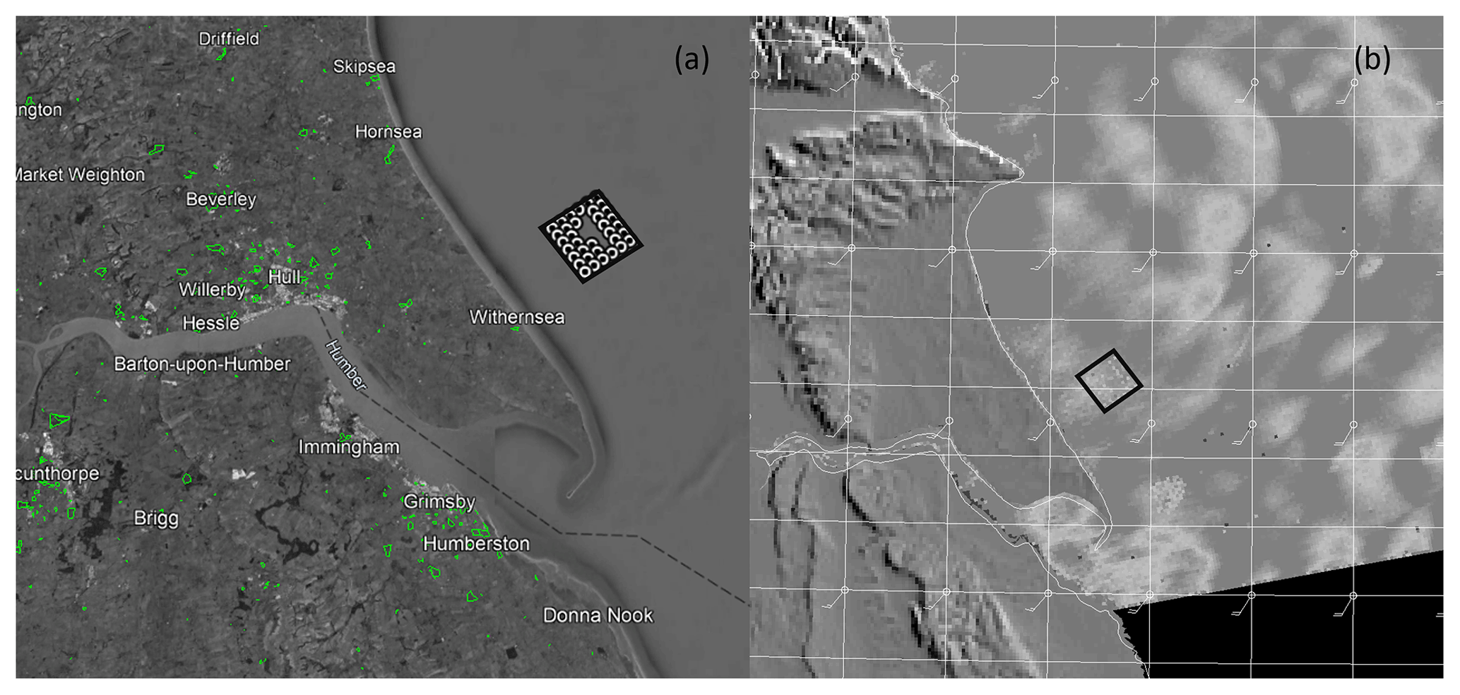
Figure 2(a) WMR location off the Holderness Coast of north-northeast England; WMR located in the black polygon (Data SIO, NOAA, U.S. Navy, NGA, GEBCO, Image Landsat/Copernicus © 2023 Google). (b) SAR image of WMR (Badger et al., 2022), raised topography shown by the darker shades of grey, and location of the WMR shown by the black polygon.
Sentinel-1a/b passed over WMR every 1–3 d in 2016–2017 around 06:15 or 17:45 UTC. The SAR images were visually inspected for TLWs in a similar manner to other studies (e.g. X. Li et al., 2013; Li, 2004; Xu et al., 2016). TLW classification of images was based on the appearance of a repeating linear pattern of fluctuating wind speeds, perpendicular to the prevailing wind direction at the location of WMR. A potential temperature vertical profile proxy for the site was taken from 97 vertical levels of ERA5 reanalysis data (Hersbach et al., 2023) for the lowest 5 km of the atmosphere. The existence of a strong temperature inversion in ERA5 was used to confirm the likelihood of TLW formation. A TLW event at WMR was selected to provide the boundary conditions for CFD simulations, and a CNBL event with a weak inversion, not strong enough to produce TLW, was selected as a control (Sect. 2.6).
2.2 Domain and topography
For all RANS simulations, Ansys CFX 18.0 was used with the Ansys WindModeller as a front end to set up the simulations. The topography includes a simplified representation of a steep near-coastal ridge, as in Ollier et al. (2018), based on a two-dimensional hill profile. The hill dimensions are based on a “witch of Agnesi” profile (Fig. 3).
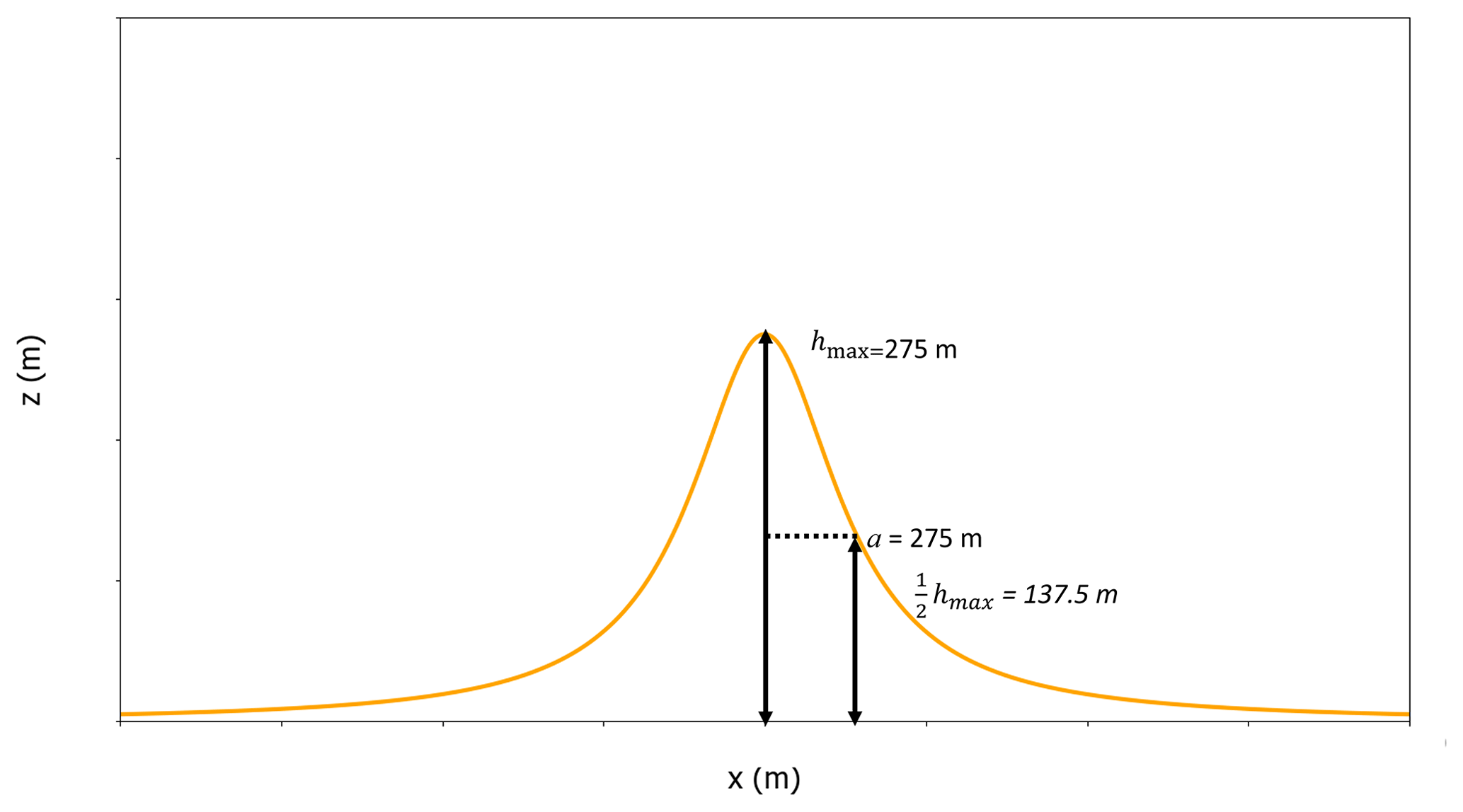
The hill height h(x) depends on the maximum hill height hmax (chosen as 275 m) and half-width at half-height a (also chosen as 275 m) as a function of horizontal distance x from the centre of the hill (Eq. 4). This results in a very steep hill, with a slope of ∼65 % (∼33∘). N.B. Flow separation is expected at slopes ≥ 30 %.
This is a very simplified hill compared to the actual topography upstream of WMR. Due to the complexity of the real terrain upstream of WMR, the simplified hill model does not attempt to capture the terrain features other than that of a simple hill, which is the same distance from the wind farm as WMR is from the coast with the aim of inducing TLWs.
This two-dimensional hill is elongated to form a ridge aligned perpendicular to the incoming westerly (270∘) wind. The hilltop is 11 km from the inlet (Fig. 4a). There is flat coastal terrain at an elevation of 10 m above sea level (a.s.l.) upstream of the ridge, with a constant roughness length (z0) of 0.03 m. The sea with constant roughness length (z0= 0.0002 m) is located downstream of the coastline as shown in Fig. 4. All domains have an upper and outlet Rayleigh damping region (Sect. 2.3).
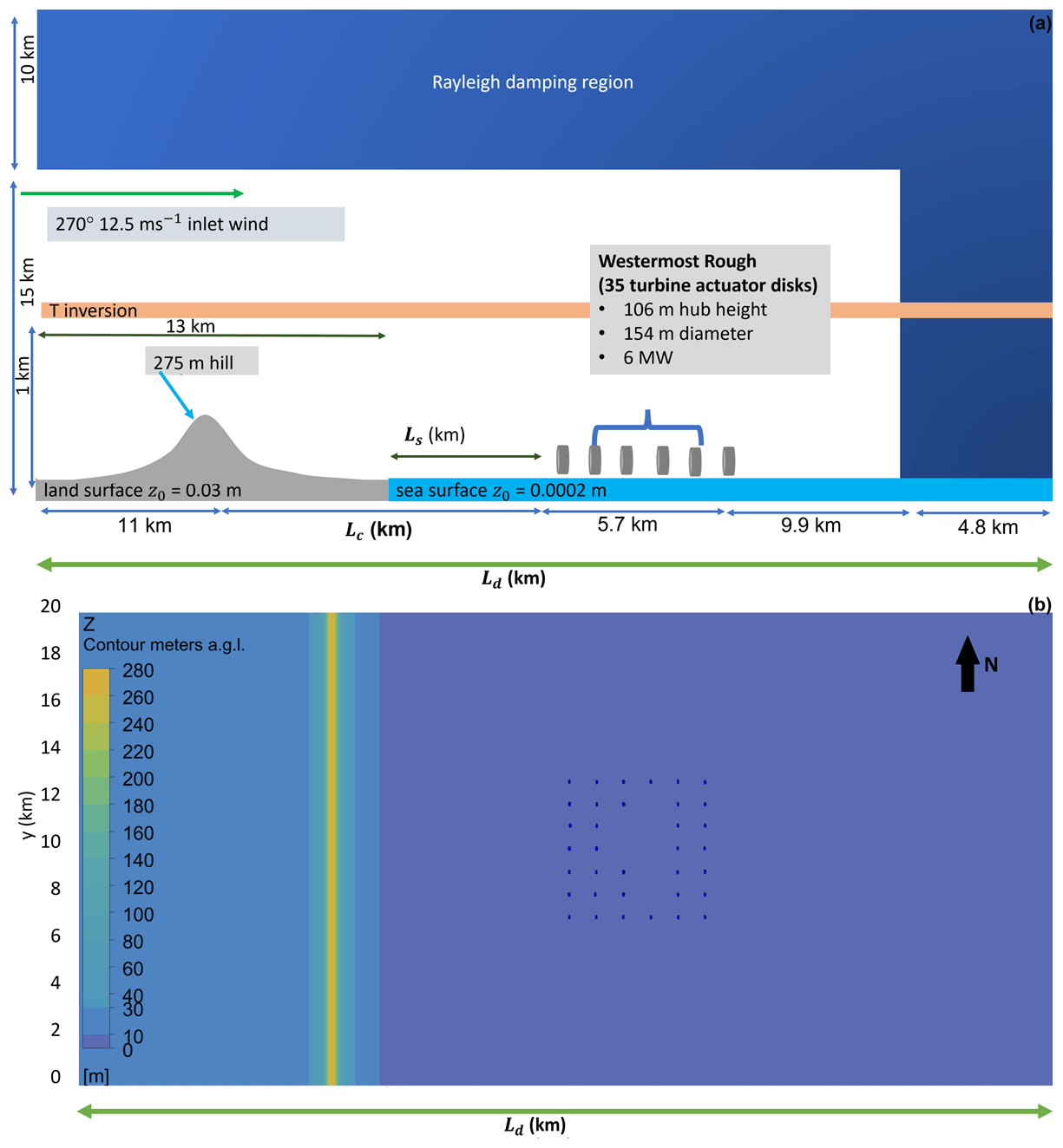
Figure 4(a) Diagram of the WM simulation domain (not to scale) for the coastal hill cases at WMR. For the 41.4 km domain, Ls,Lc, and Ld are 8, 10, and 41.4 km, respectively. For the 46 km domain, Ls,Lc, and Ld are 12.5, 14.6, and 46 km, respectively (not to scale). (b) View from WM domain for WMR coastal hill case, see legend for heights (m). Each blue dot represents a single turbine location (axes are not to scale).
To capture TLW peak interactions with WMR, a 41.4 km long domain was used (Fig. 4). This cuboid domain is 41.4 km long, 20 km wide, and 25 km high (Fig. 4). These dimensions allow for insertion of topography and downstream actuator discs representing WMR. The flow reaches equilibrium before and after these obstacles before reaching the domain boundaries. Many studies use spanwise infinite wind farms, but as Allaerts and Meyers (2017a) note, this exaggerates the blockage effect and the excitation of wind farm produced TLWs, likely overestimating their strength. The present study allows for flow transport around the model of a finite wind farm. The height of the incompressible flow domain (25 km) was chosen to avoid non-physical numerical reflections of the gravity waves (Sect. 2.3).
An extended domain of 46 km was used to assess the impact of TLWs hitting the wind farm at the trough of the TLW rather than the peak (Fig. 4). This domain follows the same layout as the 41.4 km domain, but the distance between the hill and the wind farm was extended by 4.6 km (Fig. 4), approximately half the TLW wavelength modelled in the 41.4 km domain simulations.
2.3 Wave damping
In the current work, the domain height is 3.2 λz. Rayleigh
damping at the domain boundaries was introduced to prevent unphysical wave
reflections. The damping coefficient was split into two components, τz(z), τx(x) (Eqs. 5–7), as a function of the
x and z coordinates, respectively, and damping (ξw) was added only to
the right-hand side of the z-momentum equation using Eq. (8). This was done to provide damping layers at the
top and outlet of the domain:
for ,
for x < 0,
for x≥ 0,
and for and x≥0,
The constants τ0x and τ0z (units of s−1) are set equal to 1 kg m−3 s, where ρ0 is air density at sea level (1.23 kg m−3), resulting in a maximum damping at the domain top and outlet of 0.8 s−1. x is the horizontal location in the domain (m) ( for the 41.4 km domain, Fig. 4b), rτ is the distance from the centre of the domain where damping is implemented (20.7 km for the 41.4 km domain and 23 km for the 46 km domain), Dτ is the characteristic horizontal length for which damping is applied (4.8 km, all domains, e.g. Fig. 4a), Hmax is the maximum domain height, and zτ is the characteristic vertical depth for which damping is applied. This latter value was chosen to correspond to 40 % of the domain height, i.e. 10 km, in line with a recent LES study (Allaerts and Meyers, 2017a).
In the absence of consistent guidance in the literature regarding the optimal set-up of Rayleigh damping layers, the best configuration, used for all the domains in this chapter, was based on modification of the default Rayleigh damping in the Ansys WindModeller. The damping strength was unchanged, but the location and thickness of the damping layers were modified. This was determined by trial and error. Key findings during this process were that increased domain length and depth with outflow and upper-level damping resolved most wave reflection. We did not find inflow damping helpful, and the damping layers thinner than those used were insufficient. However, these settings are specific to the dimensions, contents, and atmospheric conditions of the domain used in this research. Whilst the damping-layer strength used in this research is higher than in previous studies, Durran and Klemp (1983) found that the depth of the damping layer was more important, and the damping strength did not strongly influence the solution.
2.4 Boundary conditions
At the inlet (western plane), Dirichlet boundary conditions (i.e. prescribed profiles) were applied for the velocity vector, the potential temperature θ, and the turbulence quantities (turbulence kinetic energy k and turbulence dissipation rate ε). For the pressure, a zero-gradient condition is applied. The inlet profiles for the relevant variables were set up as follows: below the boundary-layer height, hBL, the velocity profile follows a log profile, while above it, the profile is set to the velocity value at the top of the boundary layer, VG. With the flow directed along the x axis, velocity profiles (Eqs. 9–10) were used for the velocity components (Vx, Vy, Vz):
where z0,us is the surface roughness upstream. The von Kármán constant, κ, is set to a value of 0.41. The roughness length z0 is used to set the profile by calculating the friction velocity (u*, Eq. 11). The boundary-layer height is calculated from the empirical relationship in Eq. (11) (Garratt, 1994):
with f as the Coriolis parameter ( s−1). The inlet profiles for the turbulence kinetic energy and dissipation rate are defined in Eqs. (12)–(14):
where Fcor is a roughness-dependent correction factor. The profiles for the turbulence quantities in Eqs. (12)–(14) are approximate fits to numerical results obtained for a one-dimensional simulation of a developing boundary layer over the sea after 24 h of physical time (Montavon et al., 2012, unpublished).
At the outlet (eastern plane) and at the top of the domain, an entrainment opening boundary condition is used which applies a zero-gradient condition on the velocity, zero-gradient on the potential temperature, and turbulence quantities when the flow is locally out of the domain. If the flow is entering the domain at those locations, the model then applies the same prescribed profiles as those used for the inflow. A Dirichlet boundary condition for the pressure, where the prescribed pressure profile is calculated to satisfy the hydrostatic balance associated with the potential temperature profile, is applied at the inflow1. At the sides of the domain (northern and southern planes), symmetry conditions are used for all variables. At the ground, no-slip boundary conditions are used for the velocity, using wall functions to characterize the momentum fluxes as a function of the local roughness length and friction velocity u* (ms−1, Eq. 15) (ANSYS Inc., 2021):
where Cμ is the turbulence model constant (0.09).
For neutral surface-layer simulations (Sect. 2.6), adiabatic (i.e. zero heat flux) conditions are used for the potential temperature and for the turbulence kinetic energy. Where surface stability is included, diabatic (heat flux) conditions are used for potential temperature and for the turbulence kinetic energy.
All simulations use a 270∘ 12.5 m s−1 reference wind speed at the turbine hub height (106 m). The closure for the turbulence dissipation rate at the ground is provided by ε (Eq. 13). Atmospheric stability conditions are detailed in Sect. 2.5. The Coriolis force has been shown to deflect wakes in wind farms, and wake deflection is more pronounced in the stable boundary layers (e.g. Gadde and Stevens, 2019). However, to isolate the effects of stability and the Coriolis effect, the Coriolis force is “switched off” for all simulations.
This model assumes isotropic turbulent viscosity, where the ratio of Reynolds stress and rate of deformation is equal in all directions. Whilst the κ−ϵ RANS model is less accurate in the near-wake region (e.g. Argyle, 2014), for the whole farm simulations in this research the far wake is more important. The κ−ϵ turbulence model uses modified Cμ (0.03, Eq. 15) (Montavon et al., 2011) for all simulations, as it performed best in preliminary trials, increasing the eddy viscosity in turbine wakes and reducing numerical noise in TLW simulations.
2.5 Atmospheric conditions
For the simulations including atmospheric stability, the freestream potential temperature gradient was set to K km−1 in line with the International Standard Atmosphere (International Organization for Standardization, 1975). The potential temperature profile is set as follows: for ,
for ,
and for z > zinv,
where z is height, zinv is height of the top of the inversion layer, is the inversion-layer depth, and dzinv the inversion base. is the lapse rate for the temperature inversion, and is the free atmosphere lapse rate (Ollier et al., 2018). θin is the potential temperature at the inflow, θ0 the reference potential temperature, and θ1 potential temperature for z at the inflow.
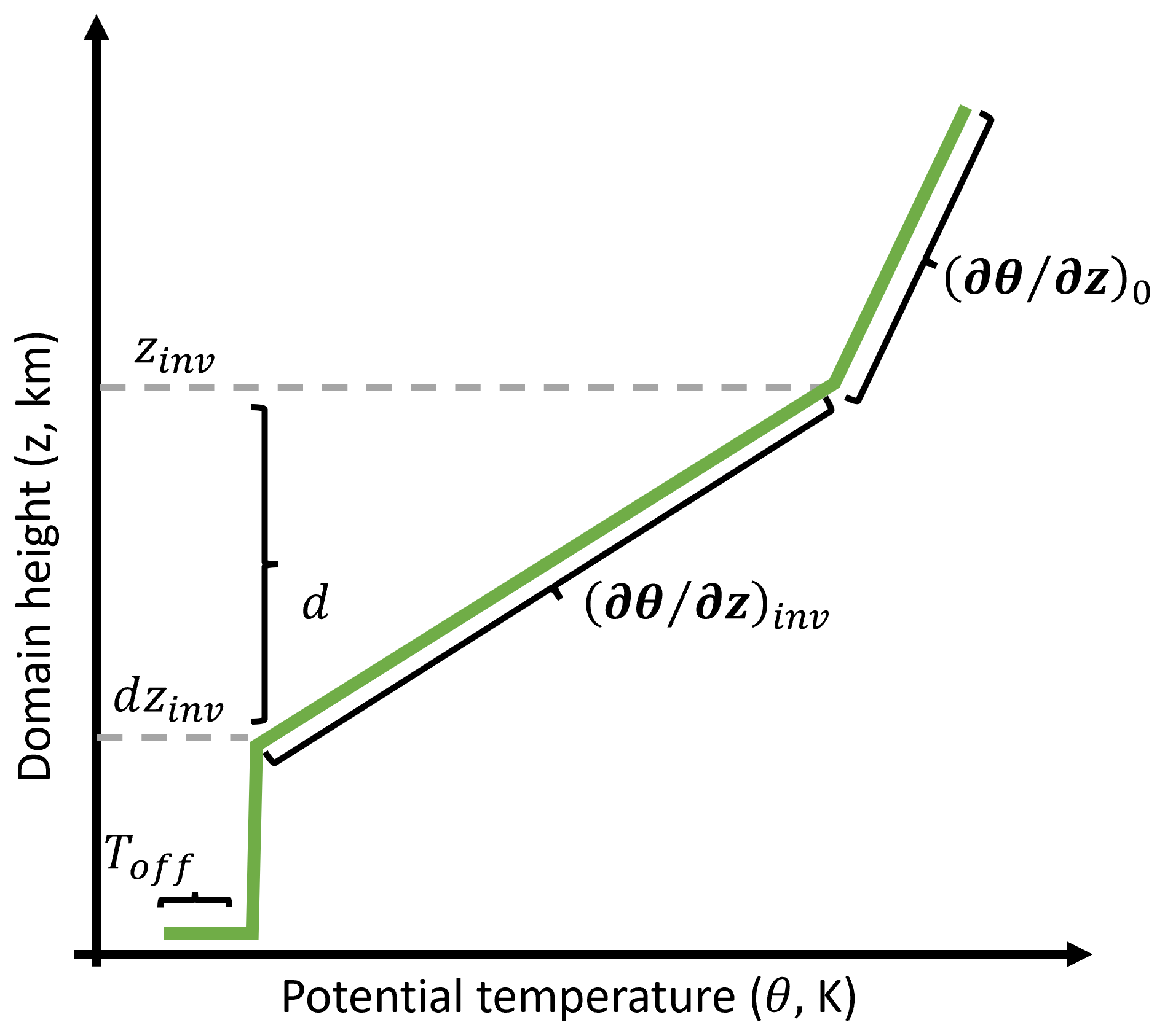
Figure 5Potential temperature schematic used in the simulations with stability where z is height, zinv is height of the top of the inversion layer, and d is the distance between the top and bottom of the inversion layer. is the lapse rate for the temperature inversion, is the lapse rate above the inversion, and Toff is the surface temperature offset.
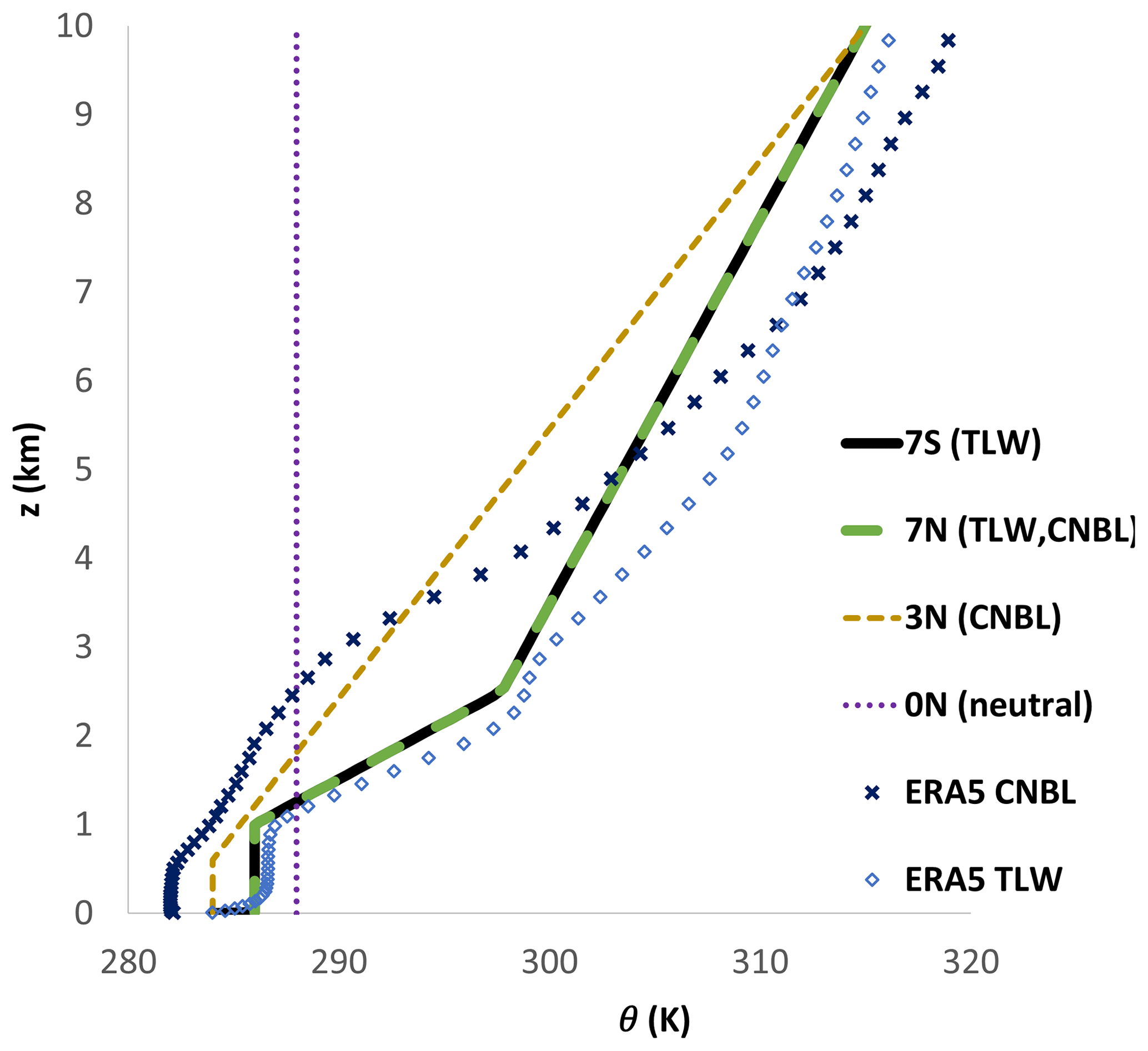
Figure 6Stability profiles from ERA5 non-TLW (CNBL) (blue cross) and TLW events (blue diamond) and WM inflow conditions approximating to the same events. Where 7S is ( 7.6 K km−1 with a stable surface layer, 7N is 7.6 K km−1 with a neutral surface layer. Additionally, 3N is 3.3 K km−1 with a neutral surface layer, and 0N is neutral throughout. Short codes summarized in Table 1.
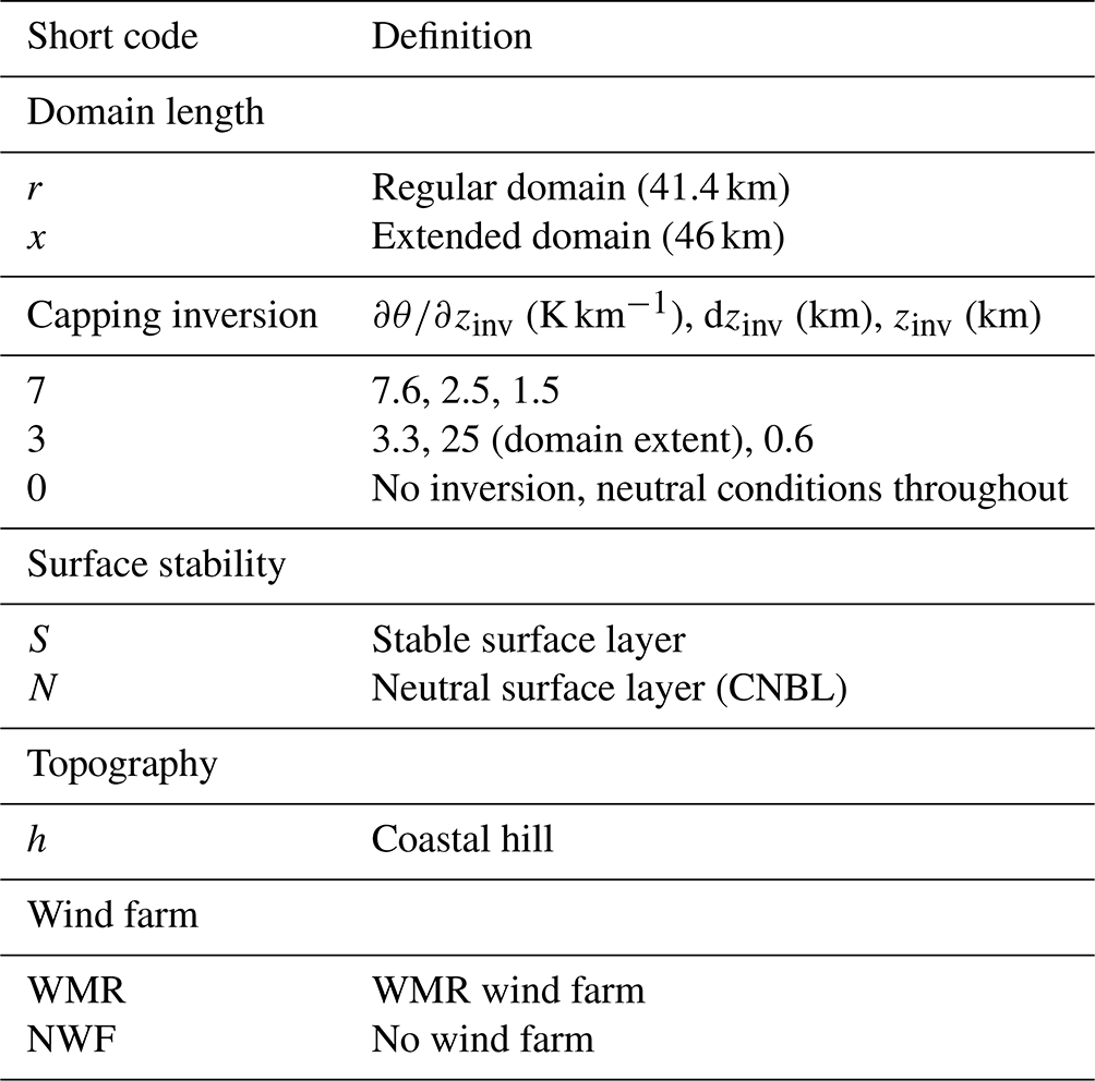
Neutral atmospheric stability was used as a control for the 41.4 and 46 km domains. In these cases, the atmospheric stability conditions were neutral throughout, with a constant potential temperature of 288 K (Ollier et al., 2018) (purple dots, Fig. 6). These simulations were given the short code “0N” (Tables 1, 2). TLW simulations included a capping inversion with lapse rate 7.6 K km−1 and a stable surface layer (short code “7S”; e.g. r7Sh-WMR, Tables 1 and 2); the temperature profile was based on the atmospheric conditions during a TLW event at WMR (Figs. 5, 6). In the ERA5 data, there was a temperature inversion around 1–2.5 km with 7.8 K km−1 (blue crosses, Fig. 6). This ERA5 profile also had a stable surface layer with approximately a −2 K surface offset, increasing to near neutral at z∼300 m. A −2 K surface temperature offset was applied in the 7S simulations, gradually increasing to neutral at z ∼ 30 m at the inlet. As the profile develops in the domain, this vertical distance increases to 300 m, comparable to the ERA5 stable surface depth. The temperature inversion was introduced using Eqs. (16)–(19) (Fig. 5, Ollier et al., 2018), with the following parameters: zinv= 2.5 km, km, 7.6 K km−1 (Figs. 5, 6) at the surface. This is the basis for proxy atmospheric conditions for TLW formation, conditioned on the potential temperature profile, wind direction, and wind speed at a reference height of 106 m (turbine hub height). To assess the impact of the stable surface layer, the same temperature inversion with a neutral surface layer was included (dashed green line, Fig. 6; r7Nh-WMR, Tables 1, 2).
For a control simulation based on real atmospheric conditions at WMR, the weak CNBL simplified profile (gold dashes, Fig. 6) was used. This is based on the weak CNBL event identified in SAR (Fig. 7b). The ERA5 data (blue crosses, Fig. 6) were taken from the same location as the capping inversion TLW case. The inversion base is at 0.6 km, with a 3.3 K km−1 lapse rate. As 3.3 K km−1 is the same as the freestream potential temperature gradient , there is not an upper limit to the inversion. These simulations were given the short code “3N” (Table 1).
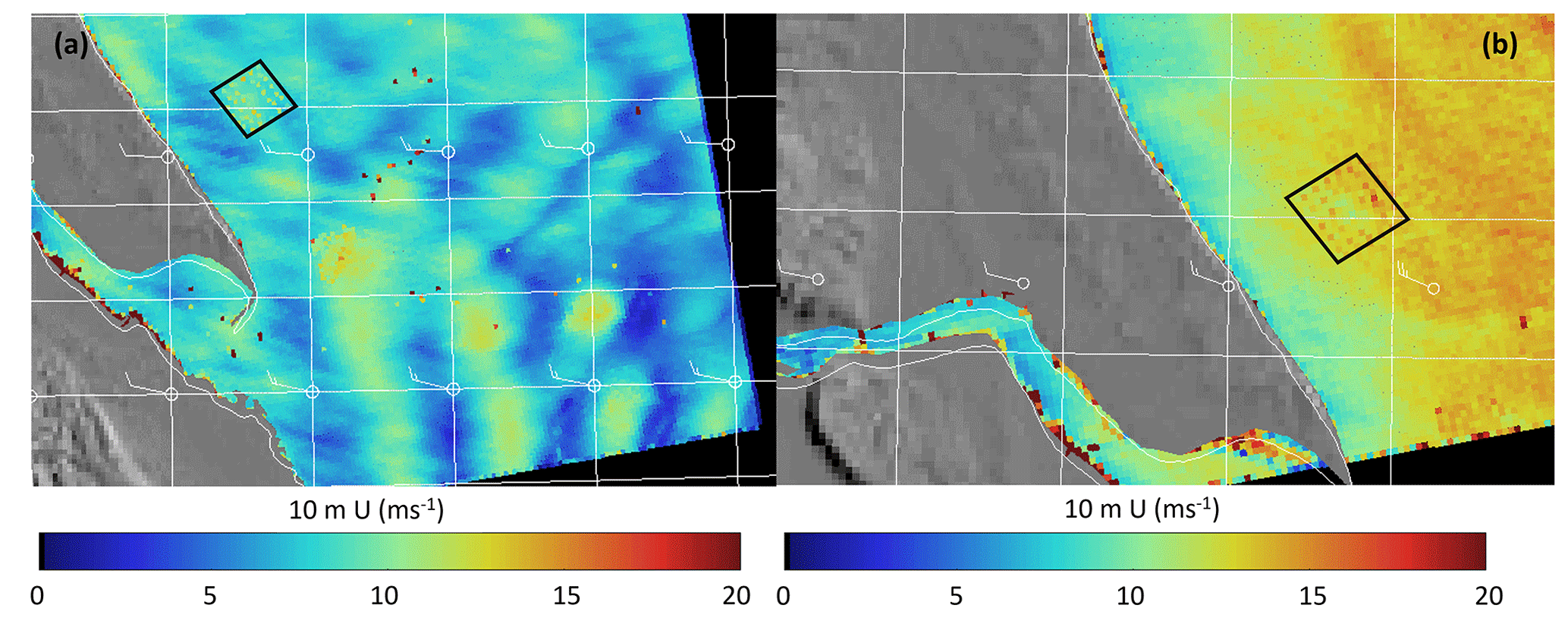
Figure 7Examples of (a) TLW and (b) non-TLW events detected in SAR images at WMR. The black square shows the location of the WMR. The legend shows 10 m wind speeds (m s−1). Images adapted from Badger et al. (2022), ENVISAT, and Sentinel-1 surface wind field processing.
2.6 Turbine set-up
The WMR layout and spacing was used for all simulations (Fig. 8). The WMR layout was rotated by 33∘ to align with the 270∘ inlet wind in the domain (Figs. 4, 8). This alignment is equivalent to southwesterly winds reaching WMR at turbine row A.
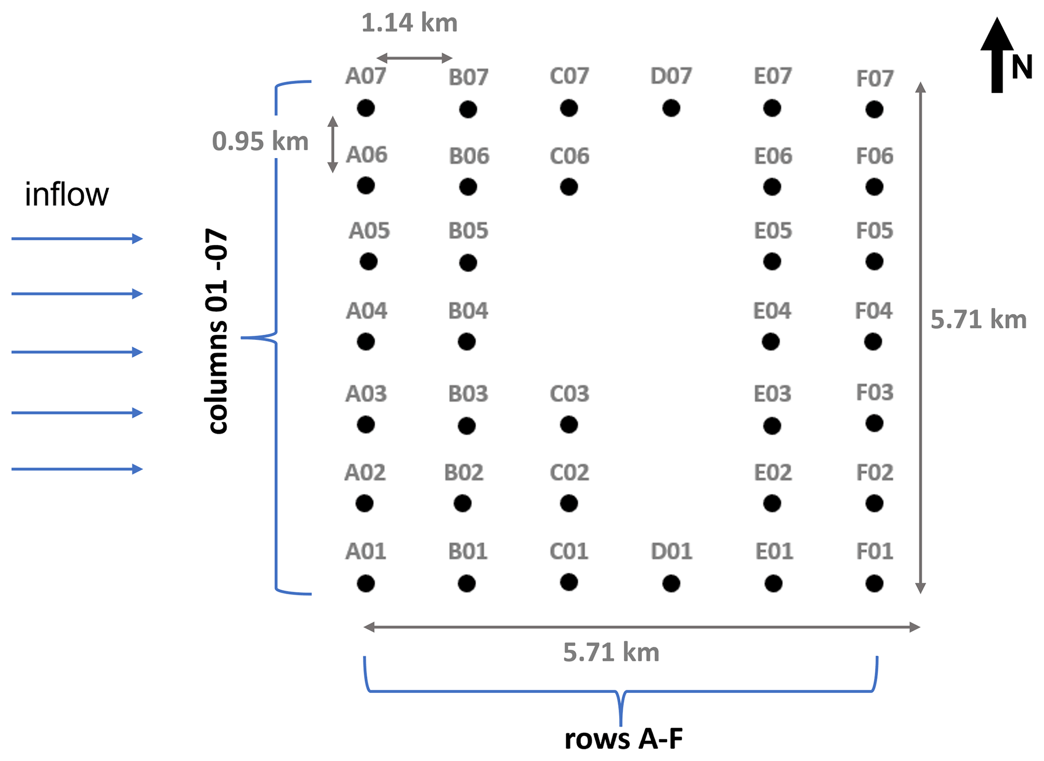
Figure 8WMR layout for the WM domain, using the same spacing as WMR but rotated 30∘ to align with the 270∘ wind direction in the domain (the equivalent of SW flow reaching WMR). Rows and columns labelled as referred to in the text.
Turbines were modelled as actuator discs (ADs), whose thrust is conditioned on the upstream wind speed, and the thrust curve is modified to be a function of disc (as opposed to freestream) wind speed. The actual hub heights (106 m), spacing (0.95 within row, 1.14 km between rows), and rotor diameters (154 m) of WMR turbines were used in this model (Fig. 8), with AD thickness ∼ 38.5 m. All turbines were set to be operational during the simulations and to yaw to the local flow direction (Ollier et al., 2018). A 6 MW, 154 m diameter turbine theoretical power curve was used with thrust data for a Siemens 3.6 MW direct drive wind turbine (SWT-3.6-107) (Appendix A). For individual turbines, local turbulence intensity is determined by Eq. (20). The freestream turbulence intensity offshore was 0.07 for all simulations.
where k is turbulent kinetic energy, and Uhub is the wind speed at the turbine hub.
Turbine Uus is obtained by using actuator disc theory to convert Uhub (Eq. 21–20) to Uus.
where:
where Uhub is the wind speed at the turbine rotor, CT is the thrust coefficient, U∞ is the freestream wind speed, and ai is the axial induction factor.
Turbine meshing was set up as in Ollier et al. (2018). The background horizontal resolution (outside of the rotor regions) for the model domain is 60 m (Appendix B). A total of 150 vertical levels were used, and the first cell above ground is 2 m thick, with a geometric mesh expansion factor of 1.15 for the levels above. For the simulations containing turbines, the WindModeller built-in mesh adaption algorithm was selected for a finer mesh around the turbines. This includes approximately 15 cells across a 154 m diameter rotor, corresponding to approximately 10.3 m per cell (Appendix B). Mesh refinement restriction was applied around the turbine actuator discs to avoid an unnecessarily fine mesh away from the turbine locations, thus reducing numerical noise and computational cost.
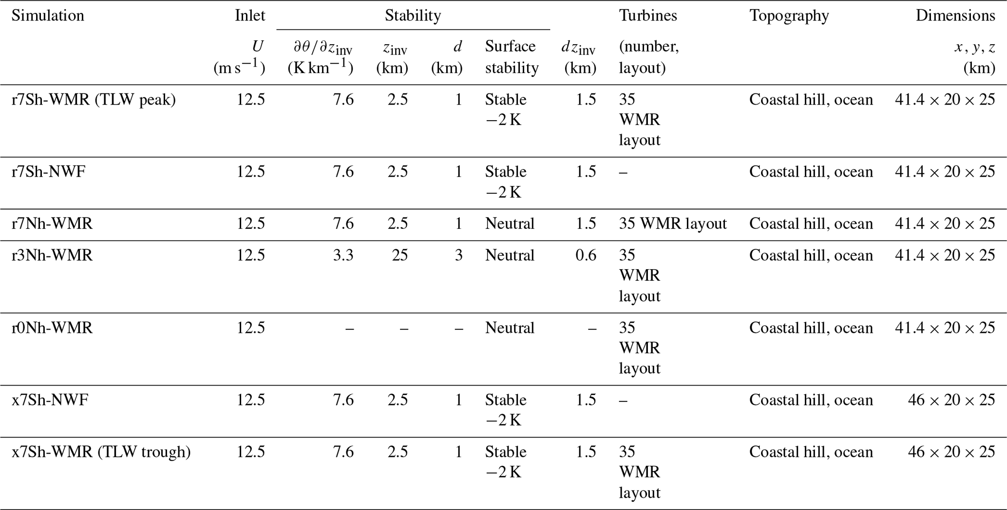
The simulations used in the current work are summarized in Table 2.
3.1 Trapped lee waves
The results from TLW simulations in this section are a snapshot from when the simulations reached a steady state with standing waves. For all simulations, the inlet wind speed is 12.5 m s−1 at a reference height of 106 m. However, the wind speeds just upstream of the wind farm vary due to flow evolution throughout the domain with differing atmospheric stability conditions interacting with terrain and turbines. For comparison of wind farm inflow conditions, near upstream wind speed (UN, Fig. 9) refers to wind speeds at a point 300 m upstream of the bottom row of WMR before the blockage effect occurs (x=0 for 41.4 km domain, Fig. 9). The wind farm blockage effect varies under the different stability conditions described in Sect. 3.1–3.3. The labels in Fig. 9 illustrate the different influences on UN.
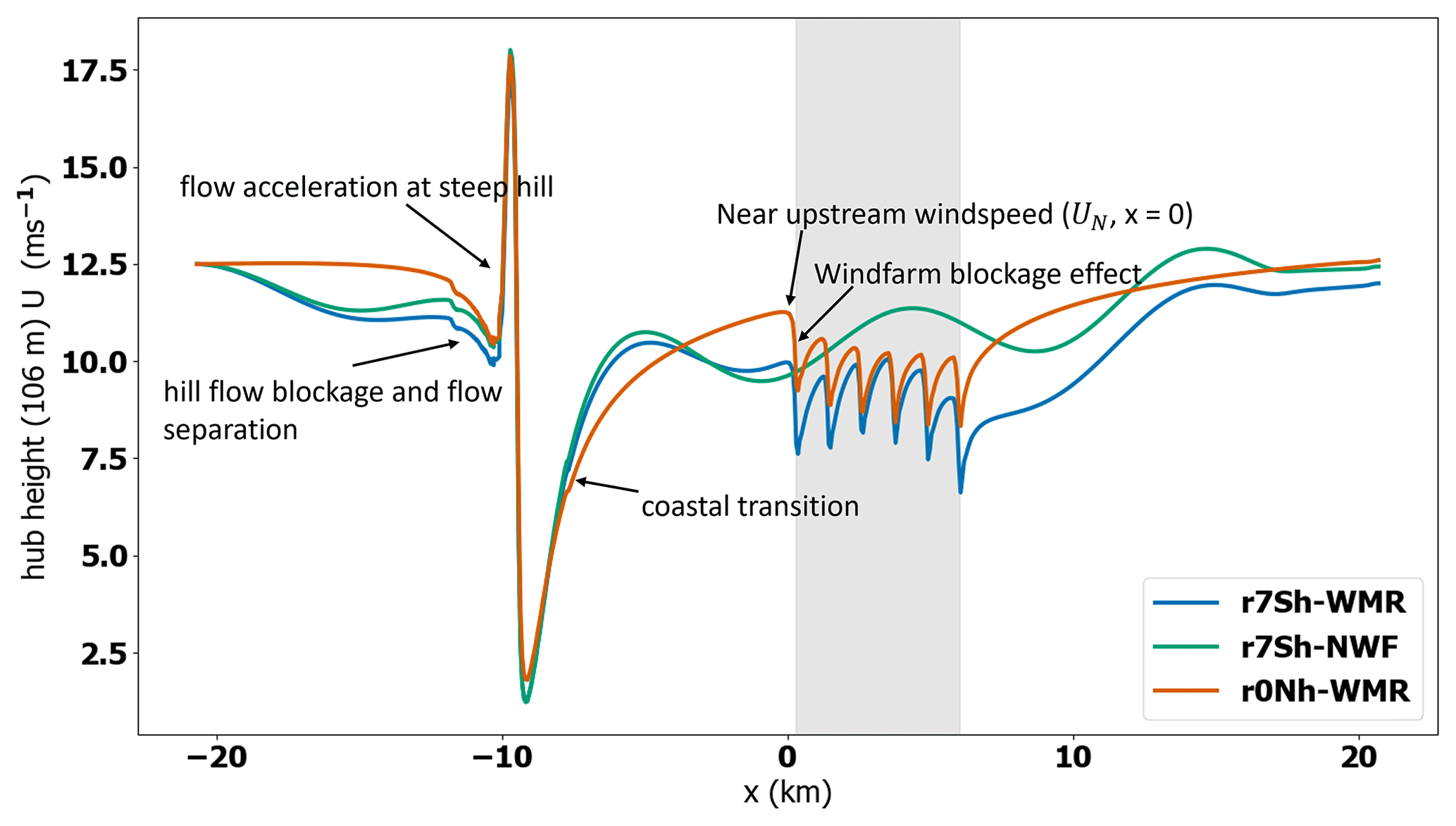
Figure 9Wind farm and stability impacts on the flow. Values are at 106 m above the surface showing the TLW peak case at WMR (r7Sh-WMR, orange line), the TLW case without a wind farm (7Sh-NWF, blue line), and the neutral control with WMR (r0Nh-WMR, green line). Grey shaded region shows the x location of WMR wind farm.
Due to the variation in the values of UN for the different simulations, direct comparisons between the simulation Uus, power, inflow angle, and turbulence intensity (TI) are complicated by different turbine thrust values. Absolute values are not compared in the current work, but the relative flow and power properties will still be influenced by differences in location on the turbine thrust and power curves at the given wind speeds. Despite this limitation, these results demonstrate topographical TLW impacts on flow patterns and consequent power outputs across WMR. Some of the influences on both UN and turbine wind speed and power which are difficult to decouple are discussed in Sect. 3.1–3.3, including recovery from the topographical blockage effect, presence of topographic TLWs, TLW phase, capping inversion and surface stability impacts, coastal transition flow adjustment impacts, presence or absence of upstream TLWs, and wind farm flow blockage effect.
For the coastal hill simulations at WMR where 7.6 K km−1 (r7Sh-WMR, r7Sh-NWF, Table 3), TLWs are observed downstream of the hill and persist throughout the domain to the outflow in both the horizontal velocity (Fig. 10a) and vertical velocity fields (Fig. 10b). Notably, there is a TLW peak upstream of the hill in Fig. 10b; TLW peaks also occurred in mathematical models of wind-farm-induced TLWs where the Froude number (Fr, Eq. 23) was less than 1 (Smith, 2010; Lanzilao and Meyers, 2021).
where U is mean wind speed (m s−1), and H is the obstacle height (m).
Table 3Simulation descriptive statistics for all WMR turbines for Uus, power, TI, inflow angle, and shear exponent factor (α).
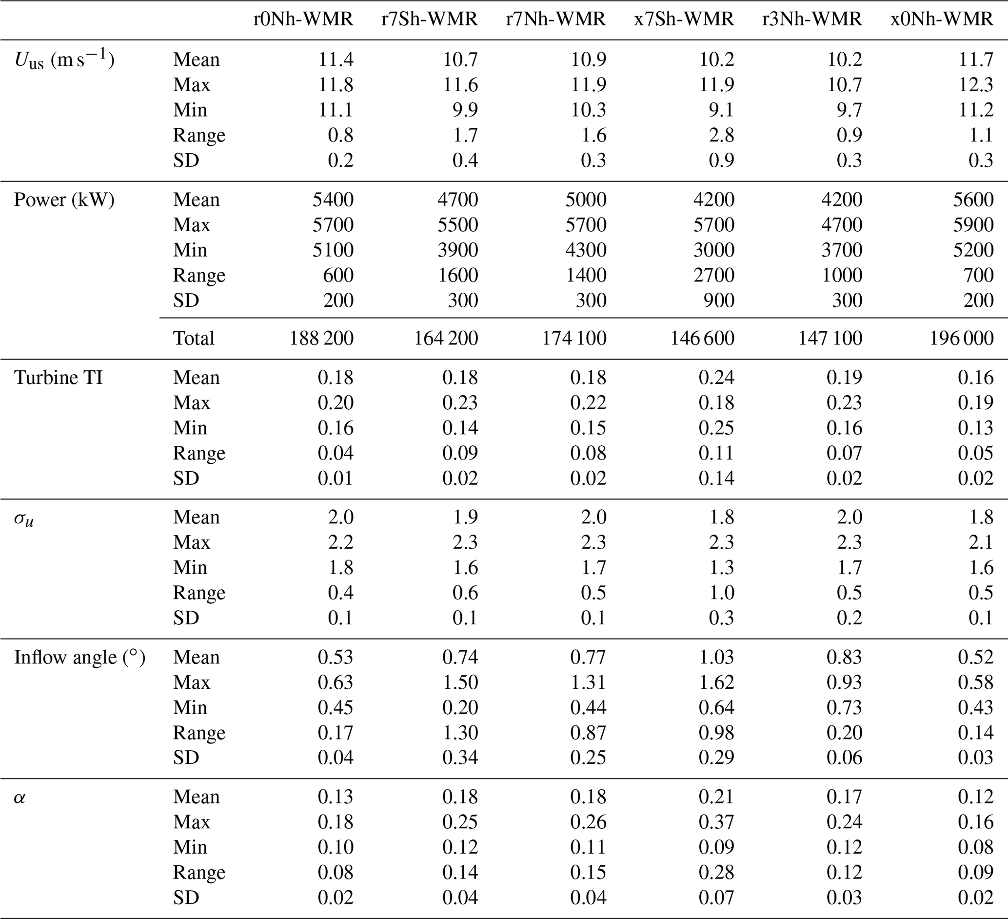
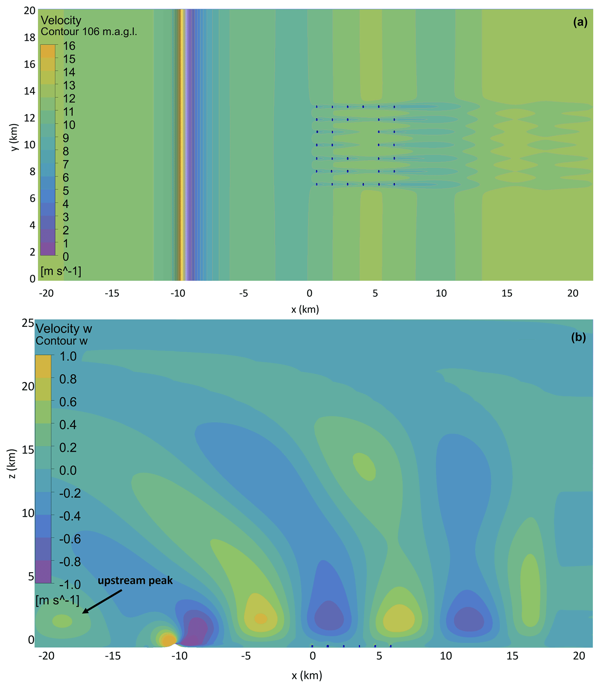
Figure 10(a) View from above: horizontal velocity at 106 m above the surface throughout the TLW (r7Sh-WMR) simulation domain. (b) Side view: vertical velocity throughout the simulation domain, the TLW (r7Sh-WMR) simulation aligned with the column 01 of WMR.
In the TLW cases (r7Sh-WMR, r7Nh-WMR) Fr ∼ 0.04, consistent with upstream wave occurrence when Fr < 1 in previous studies (Smith, 2010; Lanzilao and Meyers, 2021). However, it is unclear at this stage whether the upstream peak is an artefact of imperfect wave damping and upstream domain length. The upstream peak is, however, considered far enough upstream of the wind farm to have negligible impact on the solution at WMR. The flow decelerates rapidly on approach to the steep hill ridge (slope ∼ 33∘, Fig. 3), with acceleration and flow separation at the peak and lee side (Figs. 10, 11). The flow separation is quite severe owing to the steepness of the hill. In the 41.4 km domain, the flow is still recovering from this deceleration upon approach to WMR. The TLW is superimposed on the recovering flow and has a gradually increasing wind speed (Figs. 10, 11a). The TLW characteristics are similar for the simulations with (r7Sh-WMR) and without (r7Sh-NWF) the WMR wind farm, but the interaction with WMR results in overall lower wind speeds than when it is absent (Fig. 11a). TLW peak wind speeds are 11.4 m s−1 (r7Sh-NWF) and 10 m s−1 (r7Sh-WMR), with a mean difference of 0.94 m s−1 throughout the domain. The mean wind speed for the TLW case (r7Sh-WMR) is lower throughout the domain than for the neutral situation (r0Nh-WMR). In part this is due to the faster recovery from the hill wake in the neutral case (Fig. 11a). For reference, wind speeds for the neutral case (r0Nh-WMR) are included in Fig. 11. With a stable surface and capping inversion present (r7Sh-WMR), the flow recovery from the steep hill is slower, so the TLW begins with a much lower wind speed than the neutral case. This discrepancy in UN makes absolute comparison unclear. Further, it is not possible to fully decouple the impact of the wind farm blockage effect under a strong compared to neutral, where the blockage appears less (Fig. 11a). Two full TLW cycles are apparent in Figs. 10 and 11.
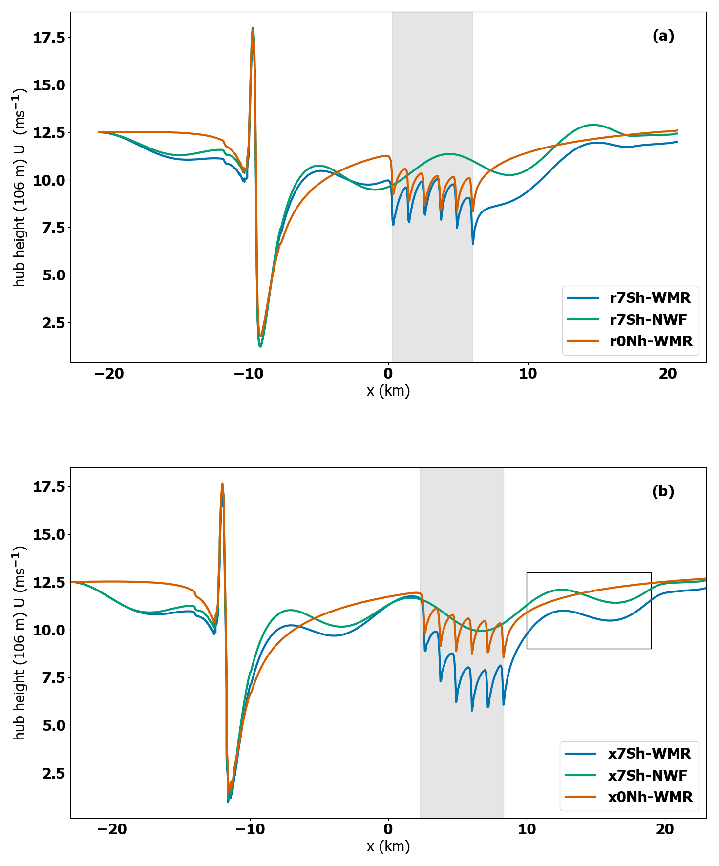
Figure 11Wind speed at 106 m above the surface U (m s−1) (a) for TLW peak with WMR (r7Sh-WMR, blue line), TLW peak without wind farm (r7Sh-NWF, green line), and neutral case with WMR (r0Nh-WMR, orange line) in the regular domain. (b) The 46 km domain for the TLW trough under the same conditions (x7Sh-WMR, x7Sh-NWR) and for the neutral case (x0Nh-WMR). The grey shaded region shows the x location of WMR wind farm. The black box highlights the area of amplitude difference between TLW simulations.
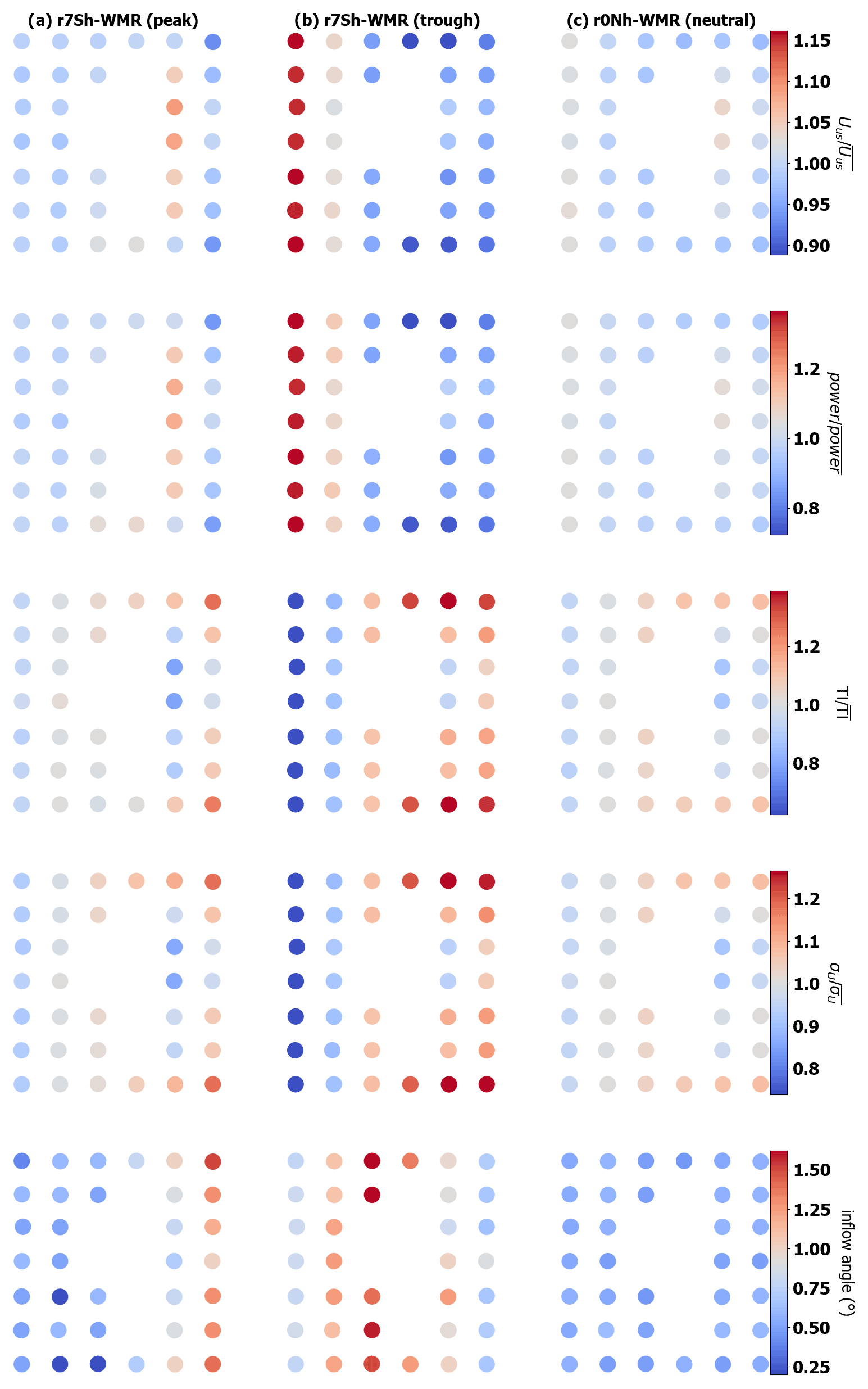
Figure 12Values normalized to the mean for all turbines for Uus (m s−1), power output, turbulence (σU), TI and inflow angle (∘) for the coastal hill domain. TLW peak (a, r7Sh-WMR), TLW trough (b, r7Nh-WMR), and neutral conditions (c, r0nh-WMR).
Here, we introduce TLW impacts at WMR at the wind farm level by reviewing individual turbine and whole wind farm flow. Whilst both the neutral and TLW cases show recovery in wind speeds after the central gap in WMR (Fig. 12), the increase in wind speeds is much higher in the TLW case. The TLW has a maximum 10 % increase in Uus (perpendicular velocity of the air cylinder upstream of the actuator disc) between turbines in row B and E either side of the gap in the TLW situation (r7Sh-WMR, Fig. 12). For the neutral situation (r0Nh-WMR) there is only a 4 % increase for the same turbine locations (Table 3). The greater recovery is explained by the increases in wind speeds due to the TLW countering wake losses. However, the central gap in WMR makes the TLW effect less clear. Furthermore, the variability in Uus throughout WMR is considerably higher for the TLW case (r7Sh-WMR) than the neutral case, with the range of wind speeds experienced by the turbines over double that of the neutral simulation (Fig. 12, Table 3). The TLW range of Uus and power output across the farm are 2.1 and 2.4 times the neutral case, respectively (Table 3). The power difference is greater due to the non-linear nature of the power and thrust curves. There are also coincident greater increases in turbulence and local TI (Eq. 20) at the turbines when the TLW is present (Fig. 12), as the trend is the same for both parameters. This is attributed to more variable vertical velocity and shear in the TLW situation, which are influenced by the coupled impacts of the TLW and the capping inversion (Appendix C).
Column 01 of WMR, where there is no gap between turbines, is less affected by adjacent columns under the 270∘ wind. This column shows the clearest TLW signature (Fig. 12a). Throughout this column, the range of Uus values is 0.9 m s−1 for the TLW case compared to 0.6 m s−1 in the neutral case. For the same locations, mean Uus is 1.2 m s− 1 less for the TLW case than neutral. The range in power output down column 01 for the TLW is over double the neutral case (1000 and 472 kW, respectively). This is due in part to differences in wind speed position on the thrust and power curves between the simulations exaggerating the wind speed differences.
3.2 Location of WMR in TLW wave cycle
Whilst the wave behaviour is similar in the 41.4 km domain (r7Sh-WMR) and the extended 46 km (x7Sh-WMR) domain, the flow characteristics at WMR are notably different depending on where the TLW hits the wind farm (Fig. 11). Turbine wind speeds and wakes in column 01 of WMR increase and decrease in phase with the TLW. In both cases, the TLW shape is clearly superimposed on the turbine wind speeds, despite the wind farm blockage effect and the fluctuation within the wind farm due to wake losses (Fig. 11). With stable surface conditions, wake recovery is slower, yet the TLW reduces the impact of the wake losses when wind speeds increase towards the peak of the wave, counteracting some of the surface stability influence (r7Sh-WMR, Fig. 11a). Wake losses are, however, amplified towards the TLW trough (x7Sh-WMR, Fig. 11b).
When the TLW is reaching its trough (x7Sh-WMR, Fig. 11b), TLW reduction in wind speeds compounds the reduction in wind speed due to the wake losses, so the wind speeds are dramatically reduced. These wind speed reductions are much more pronounced than the reductions after the TLW peak in r7Sh-WMR. This is explained by differences in nUus between simulations. The turbines in the trough case experience the trough wind speeds at a steeper location on the thrust curve, leading to deeper wake losses. At the wind farm level (Fig. 12), mean Uus is reduced relative to the neutral situation in both the peak and trough situations, as even in the peak case the first turbine row (row A) is in recovery from an upstream TLW trough. Here, with the same far upstream conditions but the TLW hitting the wind farm at a different part of the wave cycle, the range in wind speeds is 1.7 times the range for trough compared to peak case (Table 3); this difference is of the same order as the difference between the peak TLW and the neutral case. The difference in UN is 1 m s−1, so the wind speed range difference is explained mainly by the wave positioning, exaggerated by operating at a different point on the thrust curve, rather than the UN alone.
In the extended domain, the neutral simulation has a slightly higher UN compared to the TLW case (11.9 and 11.7 m s−1, respectively, Fig. 11b). This is due to the longer distance between the hill and WMR allowing for further wind speed recovery from the steep hill. Consequently, there is also a much smaller difference in Uus (mean 0.4 m s−1) in turbine column 01, between the TLW (x7Sh-WMR) and neutral case (x0Nh-WMR), than in the regular domain. Therefore, it is possible to directly compare the wind speeds between the two cases. The large range in Uus throughout WMR for the TLW situation (2.8 m s−1, x7Sh-WMR, Table 3) is mainly accounted for by the atmospheric conditions rather than differences in initial Uus, with a mean difference of 1.4 m s−1 at WMR between the two cases. The large range in Uus could be attributed to increased wake losses due to the stable surface conditions and the strong capping inversion aloft rather than the TLW itself.
At the wind farm level (Fig. 12) the TLW signature is most clearly seen down column 01 of WMR in both cases, which is less affected by the gap within the centre of the wind farm. The wave pattern is subtly apparent throughout all the turbine rows, with Uus and subsequent power output rising and falling in phase with the TLW cycle (Fig. 12). TI varies more in both the peak (TI range 0.09) and the trough cases (TI range 0.11), with both ranges over double the neutral case (TI range 0.04, Table 3). The changes in TI have a similar distribution to the changes in turbulence, suggesting that the range of turbulence is a result of vertical velocity changes in the TLW rather than wind speed differences. As the vertical velocity is more variable during TLW flows, so are the inflow angles compared to neutral conditions (see Table 3 and Fig. 12). Notably, the TI, shear, and turbulence are higher in the peak case for turbines F01 and F07; this is discussed in Appendix C.
Regardless of where in the wave cycle the TLW interacts with WMR, it recovers and the wave train persists after interaction with WMR with a slight reduction in wind speed compared to the no wind farm scenario (r7Sh-NWF, x7Sh-NWF, Fig. 11). The TLW appears to flatten at the domain outlet, but this is due the outlet wave damping. This suggests that the same topographical TLW may cause deviations from predicted power output for multiple wind farms downwind of the same hill or coastline. This is similarly discussed for onshore wind farms in Draxl et al. (2021). However, due to the domain length here, it is not possible to see how far the TLW wave trains persist and how much wind speeds recover downstream.
These results demonstrate the TLW impact on the flow, Uus, power, TI, and inflow angles throughout WMR, but to understand the impact it is essential to determine which part of the wave cycle the wind farm is in when experiencing quasi-stationary gravity waves. The impacts of the TLW will fluctuate in severity across the wind farm with TLW phase. As location in the TLW phase has such a pronounced impact, this suggests that the wind farm dimensions and turbine spacing will also be important, as they will affect how much of the wind farm is within the TLW. Similarly, the wavelength and amplitude will determine what proportion of a given wind farm is in the different TLW phases and how severe the wind speed changes are.
WMR interaction with the TLW appears to have a negligible impact on wavelength; the distance between the TLW peak in the WMR centre (grey shaded region, Fig. 11a) and the first peak after the WMR the wavelength is ∼ 10.7 km for both the WMR and NWF situation at 600 m a.s.l. away from the turbine rotors. This is also the case for the TLW trough situations. This is comparable to the wavelength predicted from the upper-layer Scorer parameter (l2, Eqs. 24–25, ∼ 12 km).
where λ is wavelength, and N= N(z), U = U(z) is the vertical profile of the horizontal wind.
There are apparent reductions in TLW amplitude where WMR is present compared to the NWF simulations. However, these differences are superimposed on flow recovery and wind farm blockage effects. The difference is most clearly observed in the black box in Fig. 11b, where the peak-trough amplitude wind speed difference is 0.7 and 0.5 m s−1 for x7Sh-NWF and x7Sh-WMR, respectively. Amplitude reduction is also observed upstream of WMR in Fig. 11a, b. As the TLW persists with reduced amplitude after interaction with WMR, this suggests that a TLW event affecting multiple farms may have less impact on wind speed and power fluctuations if there is another wind farm upstream.
3.3 Surface-layer stability impacts
Whilst the section above discusses the impact of a temperature inversion with a stable surface layer (r7Sh-WMR), this section investigates whether the stable surface layer has a strong effect on the variation of wind speeds across the wind farm. For r7Sh-WMR the stable surface layer has less impact than might be expected, as the profile becomes neutralized as it evolves through the domain (Fig. 13b). Using Monin–Obukhov similarity theory (Eq. 26) and taking across blade tip heights (29–183 m) between the inlet and hill (line 1, Fig. 13) gives 1.09 and L = 96.9 m, suggesting the flow is very stable.
where z is the height, L is the Obukhov length, and RiG is the gradient Richardson number.
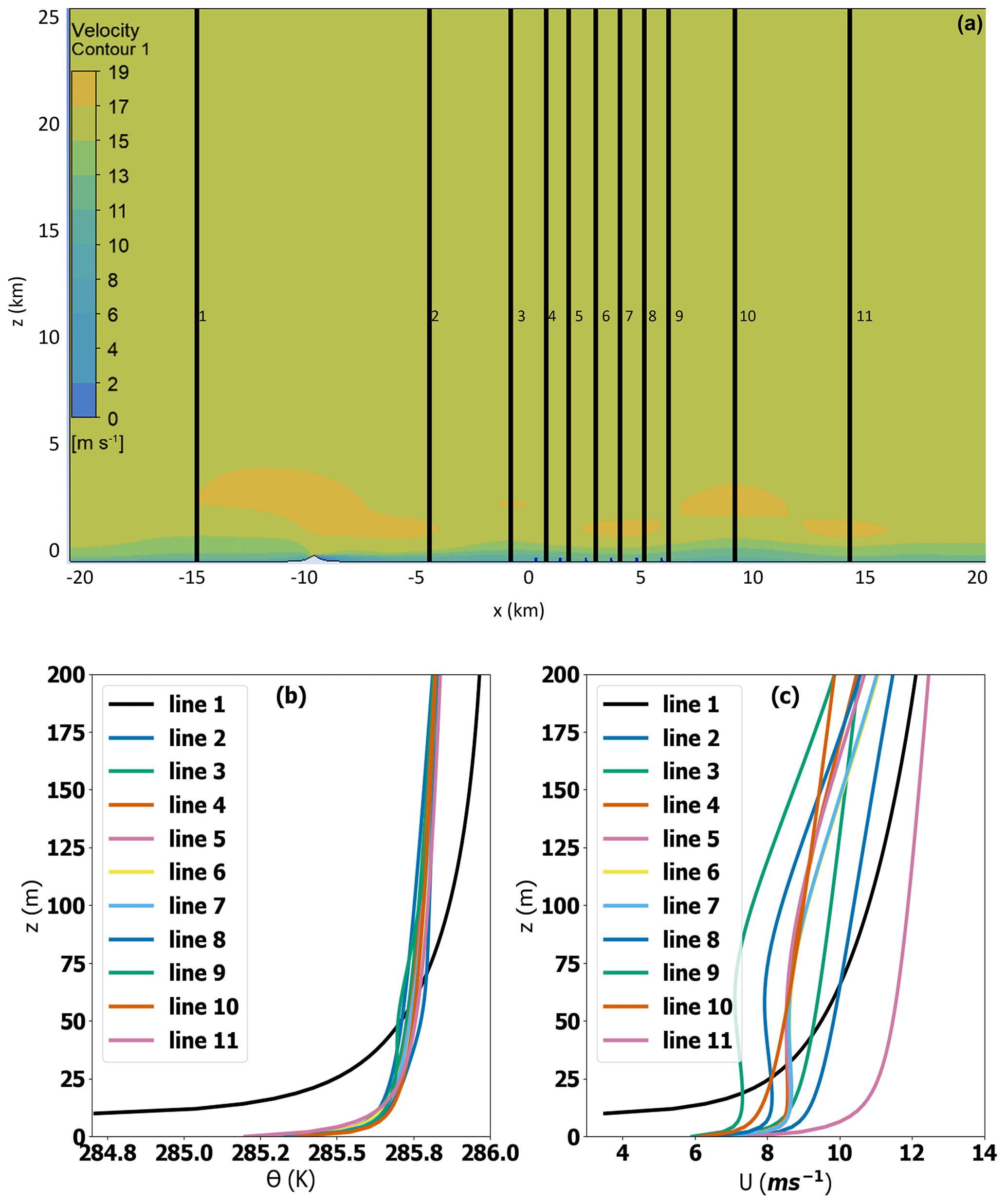
Figure 13(a) Vertical slice through the domain in line with column 01 of WMR turbines, showing vertical velocity for the TLW case (r7Sh-WMR). Black lines represent lines 1–11, as labelled in all three plots. Below: WM potential temperature (b) and velocity (c) profile for lines 1–11.
Yet the stability profile has a relatively subtle temperature offset once the inlet profile has adjusted within the domain and interacted with the topography to a relatively small temperature offset (< 1 K) and shallower surface layer (lines 2–11, Fig. 13b). Changes in velocity profile after the topography may be attributed to TLW trough flow effects on shear and associated turbulence, as described in Vosper et al. (2018). To obtain a temperature profile with strong stability at WMR the WindModeller inlet surface temperature offset would need to be increased to counteract the neutralization in the domain.
As shown in Fig. 14, the flow throughout the domain is similar for both the inversion case with the neutral surface layer (r7Nh-WMR) and the stable surface layer (r7Sh-WMR). With the stable surface layer (r7Sh-WMR), mean Uus and power are reduced, with increased wake losses slightly increasing the wind speed reduction effect of the TLW. This leads to negligible increases in variation in Uus, with a range of Uus which is 0.07 m s−1 greater for r7Sh-WMR than for the neutral surface layer (r7Nh-WMR) with resulting power output variation range of 1592 kW (for r7Sh-WMR) and 1435 kW (for r7Nh-WMR) (Table 3, Figs. 14, 15).
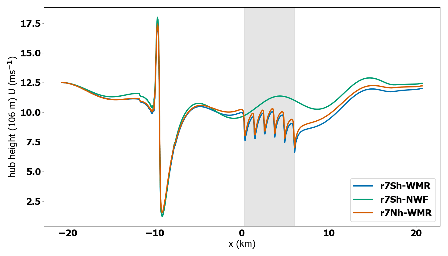
Figure 14Height of 106 m above the surface isolines of U aligned with column 01 of WMR for capping inversions with (r7Sh-WMR, orange line) and without (r7Nh-WMR, blue line) stable surface conditions and stable surface conditions without WMR (r7Sh-NWF, green line).
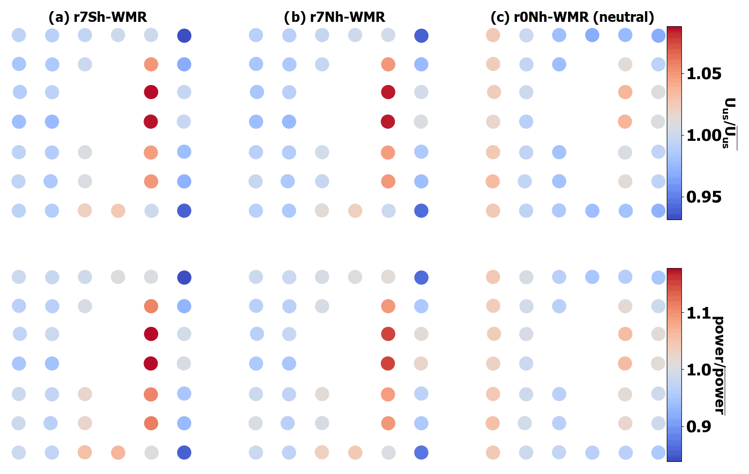
Figure 15View from above the WMR, normalized to the mean value for WMR for Uus and power output (kW) for the TLW peak (column 01, r7Sh-WMR), TLW peak CNBL (b, r7Nh-WMR), and neutral (c, r0Nh-WMR) cases.
The influence of the TLW dominates with a slight reduction in the range of values for all variables for r7Nh-WMR compared to the stable surface-layer case (r7Sh-WMR, Table 3). Figure 15 compares the whole wind farm for the stable surface and neutral surface cases (power, TI, Uus) with neutral conditions for the regular domain. As the surface stability temperature offset reduces substantially after interaction with the topography and sea surface (lines 2–11, Fig. 13), the stable layer is relatively shallow with the surface lapse rate increasing to near-neutral conditions around rotor height. Thus, the differences between r7Sh-WMR and r7Nh-WMR are relatively subtle. In these situations, the impact of the capping inversion appears much more important than the surface stability. Yet, much larger differences between the stable and neutral surface-layer simulations would be expected, with a stronger and deeper stable layer at the surface which would increase wake losses further.
3.4 TLW compared to CNBL conditions at WMR
The CNBL case (r3Nh-WMR) is a more realistic atmospheric situation than purely neutral conditions (r0Nh-WMR). In Fig. 16a UN for r3Nh-WMR is substantially higher than for the TLW peak situation (r7Sh-WMR, 10.9 and 9.6 m s−1, respectively, at x= 0). However, the gradual decline in wind speeds due to wake losses reduces Uus throughout WMR to less than those for the TLW situation (r7Sh-WMR, b), where the losses are countered by the peak of the TLW. The reduced wind speed in the CNBL case (r3Nh-WMR) results in a lower position on the power curve, resulting in a reduced power output across WMR compared to the TLW peak and neutral cases (Fig. 16). Whilst Uus and power are more variable for the TLW situation (r7Sh-WMR, range 1.8 and 2.7 times greater, respectively, Table 3) than for the CNBL, the total power output is only 1.1 times lower for the CNBL case (r3Nh-WMR) due to its higher UN. Whilst these differences are small, if UN were equal for both cases, i.e. different far upstream wind speed, the TLW would cause more dramatic increases in power output compared to the control as the initial offset between the two cases would be removed. Uus and power increases would be expected, as the peak increases are not counter-balanced by the TLW troughs, as WMR is small and is not experiencing the lowest speeds in the TLW trough in this situation (Fig. 16). Not accounting for differences in atmospheric stability and TLW impacts could result in over- or underestimation of power output when based on a mast measurement alone.
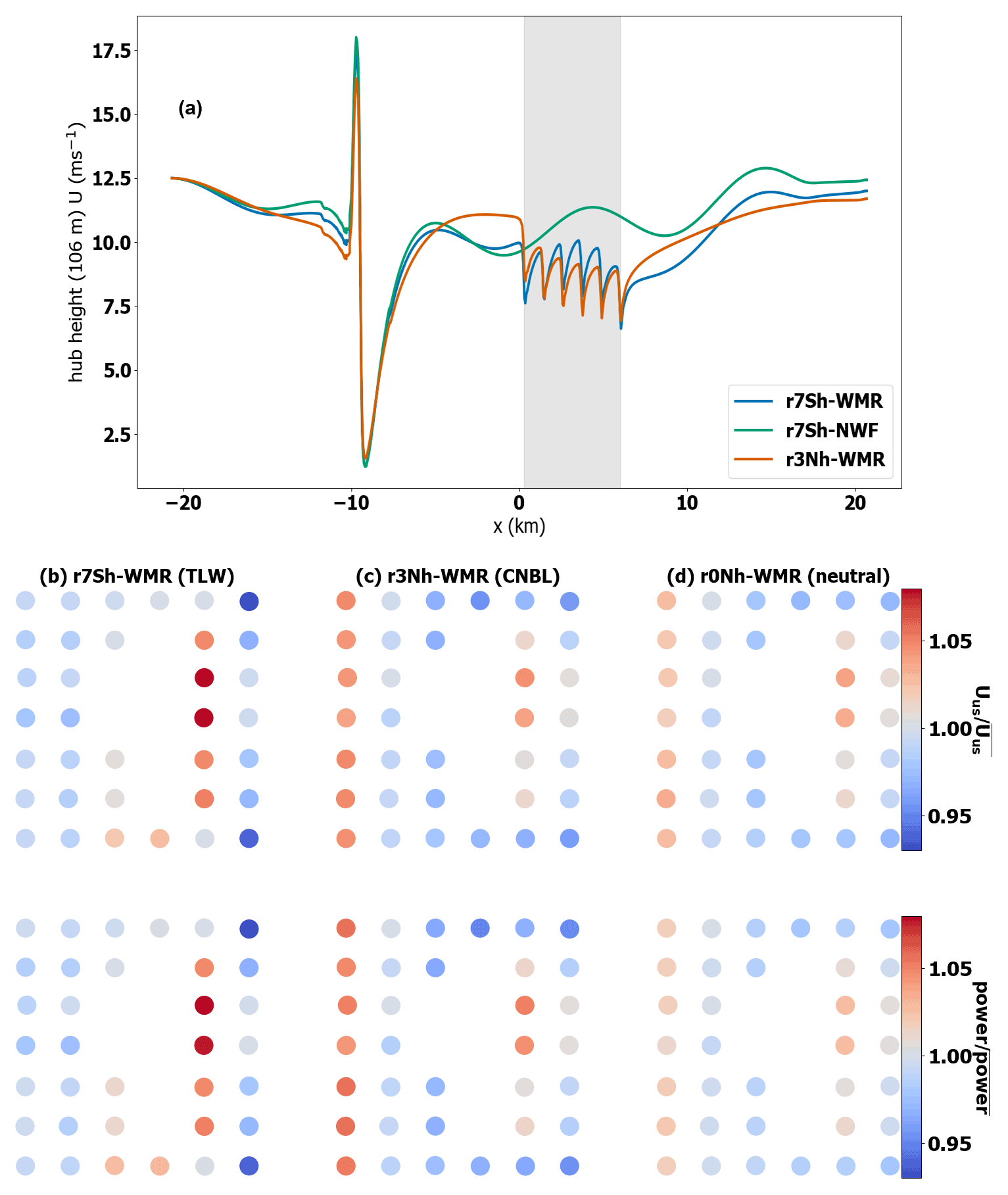
Figure 16(a) Hub height wind speed aligned with column 01 of WMR for TLW (r7Sh-WMR, blue line), TLW without WMR (r7sh-NWF, orange line), and weak CNBL case (r3Nh-WMR, green line). Below: normalized Uus and power for WMR for TLW (b, r7Sh-WMR), CNBL (c, r3Nh-WMR), and neutral cases (d, r0Nh-WMR).
The CNBL case is approximated to real conditions at WMR so is more representative than the purely neutral conditions; however, what constitutes a true control for TLW situations is unclear. Here, the CNBL has a shallow and weak inversion. Modifications to height, depth, and strength of inversion layers will produce different wind speeds and turbulence throughout the domain and interact differently with individual turbines and whole wind farms. As discussed in Sect. 5, investigating TLWs using a variety of stability profiles, and producing control simulations with varying profiles and similar near upstream wind speeds would be beneficial for full quantification of TLW impact.
3.5 Impact of TLW on potential turbine loading for topographical TLW simulations
For all the topographical TLW simulations at WMR (r7Sh-WMR, r7Nh-WMR, x7Sh-WMR), the range of inflow angles is larger than for the neutral equivalents (r0Nh-WMR, x0Nh-WMR, Fig. 12). The mean inflow angle is largest for the TLW trough simulation (x7Sh-WMR), where it is almost double that of the neutral equivalent (x0Nh-WMR) (mean 1.03 and 0.52∘, range 0.98 and 0.14∘, respectively, Table 3). Whilst the TLW inflow values are higher, they are well within the tolerance range of modern wind turbines (∘), so turbine fatigue loading does not seem to be a concern for these conditions. The TLW trough simulation (x7Sh-WMR) also shows the largest difference in turbine TI compared to the neutral case (r0Nh-WMR, mean 0.24, 0.16, range 0.11, 0.05, respectively). As the trends in turbulence and TI match, the changes in TI are likely a result of shear associated with up- and downslope TLW flow.
Whilst this research focuses on the impact of TLWs on Uus and power output, larger inflow angles, greater TI, and associated shear suggest that some turbines across the wind farm are likely to experience greater fatigue loading during TLW events and that this is not uniform across the wind farm. However, these increases in inflow angle and TI do not appear large enough to substantially impact turbine fatigue and lifetimes.
Topographical TLW interaction with wind farms is common and has, until recently, been overlooked (Ollier et al., 2018; Ollier, 2022). In this parametric study, turbine and whole wind farm wind speeds and power outputs behaved differently in the presence of topographically forced TLWs. In the simulations, the reference wind speed at the inlet was analogous to a mast measurement taken 20 km upstream of a proposed wind farm site. In the presence of an upper-layer inversion, strong TLWs meant that the topographical influence was more apparent. These results demonstrate that with the same apparent synoptic forcing conditions, local conditions favouring TLW formation may lead to large deviations between the predicted and actual wind speed. Thus, power output from individual turbines and whole farms will vary significantly from predicted if these conditions are not accounted for. Greater variability in local turbulence and shear was also apparent during TLW situations attributed to TLW and capping inversion impacts on wake and shear. However, the TLW impact on inflow angles within WMR was well within the tolerance of modern wind turbines. TLW events affecting multiple wind farms may have less impact on power output for wind farms downstream of an existing wind farm due to appreciable reductions in TLW amplitude with wind farm interaction.
The different atmospheric stability conditions led to the same upstream flow conditions interacting very differently with the topography upstream of the wind farms. Consequently, wind farm inflow speeds were highly variable between TLW and non-TLW events, leading to differences in wind speed throughout the wind farm. These differences were further complicated by the varying wind speed recovery from the coastal transition and differences in wind farm blockage effects in different stability regimes. Additionally, wake recovery appeared dependent on both the TLWs and strength of the capping inversions. With these interacting conditions it was not possible to fully decouple which impacts on wind turbine and whole wind farm wind speeds and power were a result of TLWs and which were a result of different stability impacts on the flow.
When compared to purely neutral conditions throughout the domain, all the TLW simulations had reduced power output. These reduced speeds compared to neutral for TLW simulations were primarily due to reduced flow recovery after the hill due to stability differences. As it was not possible to define consistent wind farm inflow conditions between TLW and control simulations, it remains unclear how much of this influence was due to TLWs compared to impact of differing UN. The effect will be situation dependent, as differences in UN lead to different operating points on the thrust curve and non-linear changes in wake losses. Yet, when compared to a non-TLW CNBL event at WMR, with higher UN than the TLW, subtle increases in turbine Uus and turbine–whole wind farm power output were observed during the TLW. This suggests that TLWs may sometimes have beneficial impacts compared to real CNBL conditions. How the TLW impact is interpreted is largely based on what is taken as the “control” situation. In all simulated cases, TLW events increased the variability in wind speeds and power outputs through the wind farm. Despite the variation in UN which complicates the interpretation of the results, it is concluded that TLWs can have a substantial impact on the variation in wind speeds and TI experienced across an offshore wind farm and the resulting power output of individual wind turbines.
The location of the wind farm in the wave cycle was an important factor in determining the magnitude of TLW impacts. TLW peaks countered wake losses, and TLW troughs enhanced them. There were greater ranges of wind speed and power output during TLW events; the range was greater for TLW troughs than peak cases at WMR. Trough wind speeds were, however, coincident with operating points on the power and thrust curves where wake losses were greater. Whether TLW impacts are beneficial, detrimental, or balance out will be dependent on the wind farm location within the TLW wave cycle, wind farm dimensions relative to the TLW wavelength and amplitude, TLW wavelength, TLW amplitude, and TLW orientation in relation to the wind farm dimensions. Whether the wave is quasi-stationary or travelling will also have an impact. A travelling TLW will have transient impacts on turbine outputs that may cancel out overall, whilst quasi-stationary waves may lead to longer-term differences compared to predicted power output. Again, the interpretation of TLW impact for all wind farm sizes will largely be determined by what reference conditions the TLW conditions are compared to. For example, when compared to purely neutral conditions (not existing in reality), TLWs may lead to power output improvements compared to real atmospheric non-TLW situations for the same value of UN. Without a constant UN between simulations, it was not possible to determine whether there was a balancing effect across the wind farm. Furthermore, it is not yet known whether multiple TLW events at the same wind farm may balance out over a longer period.
In the current work, it remains unclear how much contribution the following conditions make in TLW situations: (i) differences in initial UN, (ii) wind speed recovery from topographical obstacles, (iii) flow adaptation to roughness and temperature changes after the land–sea transition, (iv) wind farm flow blockage, (v) TLW phase, (vi) height and strength of the inversion layer, and (vii) presence of surface and/or upper-level stability. Further work to obtain consistent UN would help quantify influences of the other variables listed above. Whilst subtle differences were found between the stable and neutral surface-layer TLW conditions in the current work, applying a variety of surface stability conditions would provide a clearer understanding of the interaction between TLWs and the surface conditions. Further work to determine the relative contributions to wake recovery by the stable surface layer and the capping inversion aloft would need to first address the evolution of the stable surface layer from the inlet to the wind farm. This may be achieved by a considerably longer upstream domain length and exaggerated upstream surface stability. Additionally, varying the inlet wind speed and direction, inversion strength, depth and height, topography dimensions, and orientation would help determine their contributions to TLW impacts. It is recommended that future investigations use a variety of wind farm layouts to investigate wake recovery under TLW conditions. Additionally, future investigations into TLWs would benefit from systematic adjustment of wave damping and domain dimension parameters to develop guidelines for optimum wave damping set-up.
In the current work, high-resolution SCADA (supervisory control and data acquisition) data were not available for demonstrating the impact of TLW in a real operational wind farm. Thus, this is a priority for future TLW investigations. For a fuller description of real atmospheric TLW wind farm interactions moving forward, combined use of CFD, lidar, high-temporal-resolution SCADA, and high-resolution mesoscale modelling to downscale ERA5 data is recommended. These methods would enable improved spatial and temporal description of TLW characteristics, which could then be utilized to assess the impact of TLWs on wind farms. Assessing different TLWs would provide information on the dependence of impacts on the TLW characteristics. Now that theoretical TLW wind farm impacts have been demonstrated, developing models for larger wind farms and existing wind farm clusters will demonstrate the impact of greater spatial interaction with TLWs. Whilst it may be possible to model a longer domain length in CFD, a coupled micro–mesoscale model would be more appropriate for this large problem. With larger wind farms, a stronger influence on TLW amplitude is expected, which may enhance or reduce the wind speed fluctuations for downstream wind farms.
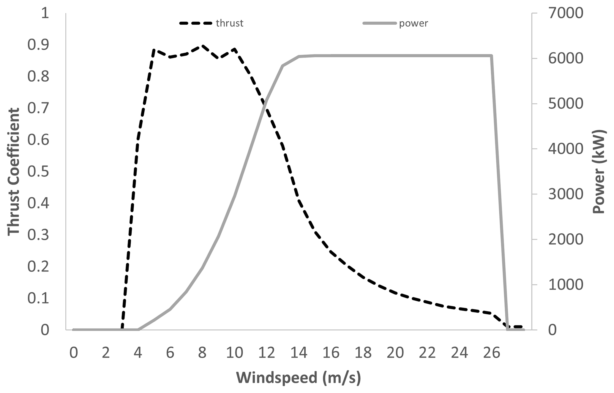
Figure A1Thrust coefficient and power curve data used for the 6 MW 154 m diameter turbines in the simulations.
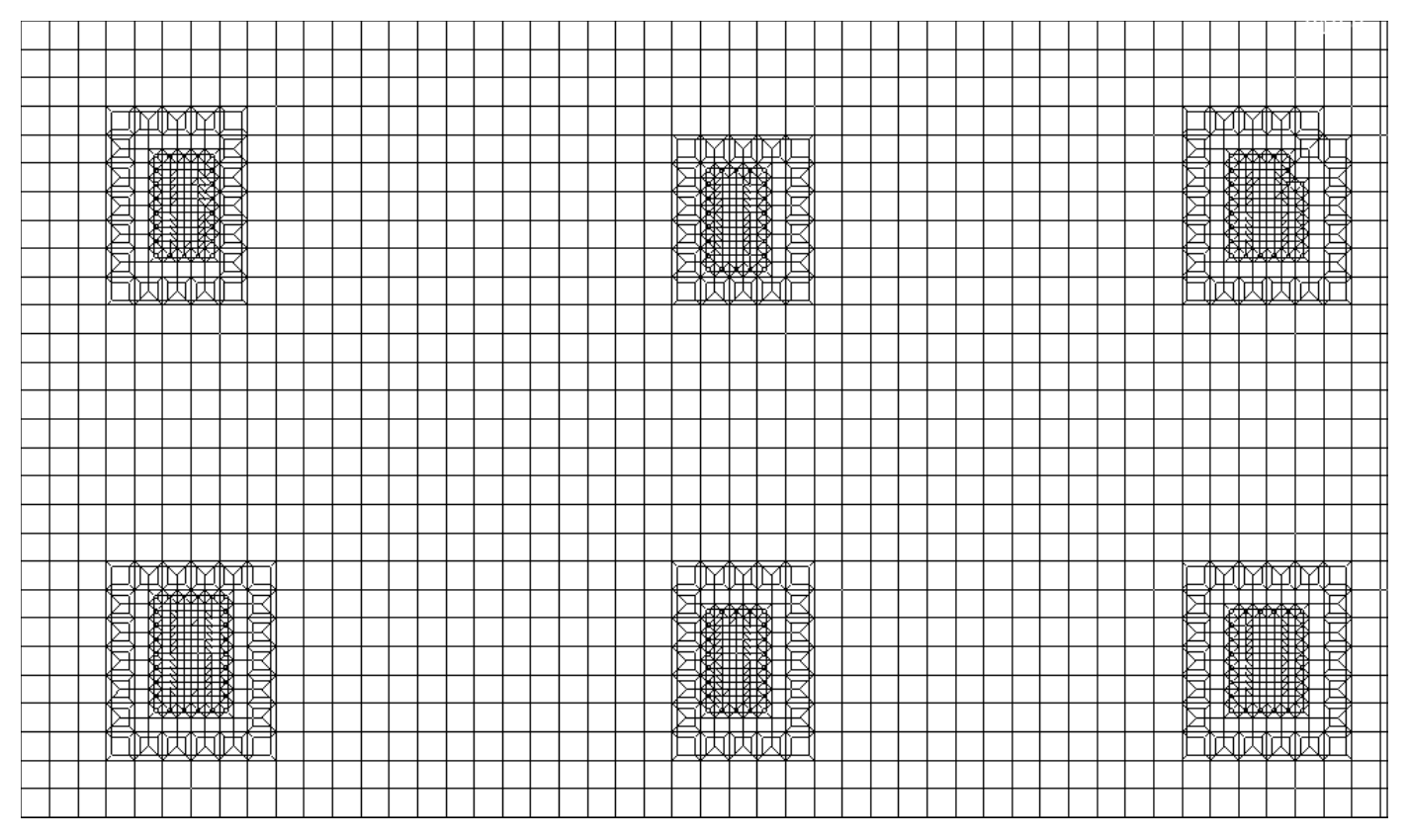
Figure B1Horizontal mesh structure for the WMR wind farm region of simulation domain at turbine hub height (106 m) used for all simulations. The mesh refinement around each actuator disc is shown in the darker regions. Note that the mesh refinement around individual turbines leads to asymmetrical meshes for some turbines.
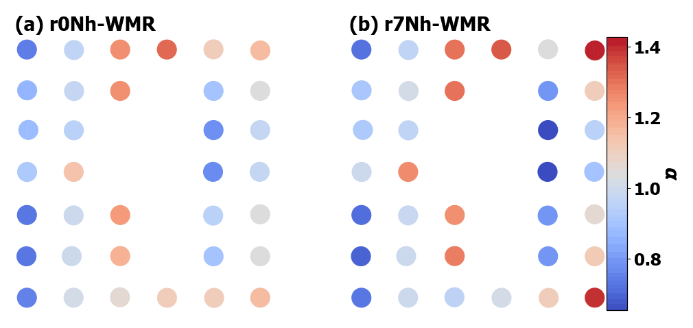
Figure C1 shows the shear exponent factor (α) for the neutral case (r0Nh-WMR) and the TLW case with a neutral surface layer (r7Nh-WMR). Shear is more variable within the TLW case, where there are deeper near-wake losses (Figs. C2, C3). The greatest shear variability is experienced by F01 and F07, which experience the deepest near-wake losses and TI (Fig. C3) due to having a full column of turbines upstream. For the TLW case the wakes and elevated wake TI persist further downstream into the wave damping region. The impact of the TLW and the capping inversion are coupled, so it is unclear which has a greater influence on the shear, turbulence, and near-wake loss depth.
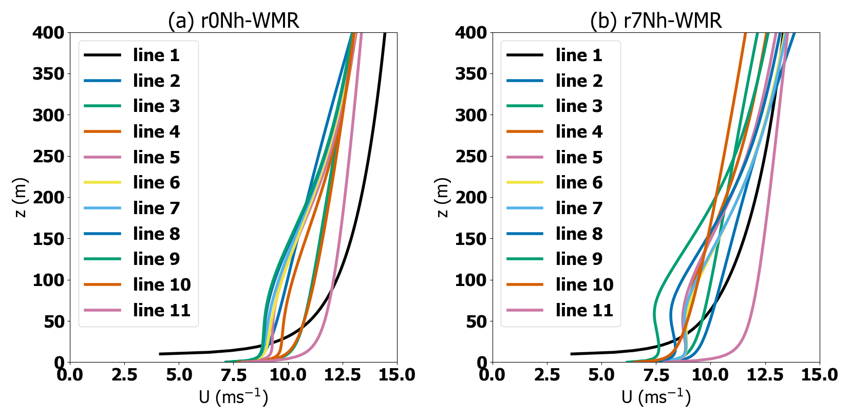
Figure C1Vertical wind speed profiles for (a) r0Nh-WMR and (b) r7Nh-WMR. Numbered lines correspond to lines 1–11, labelled in Fig. 13a.
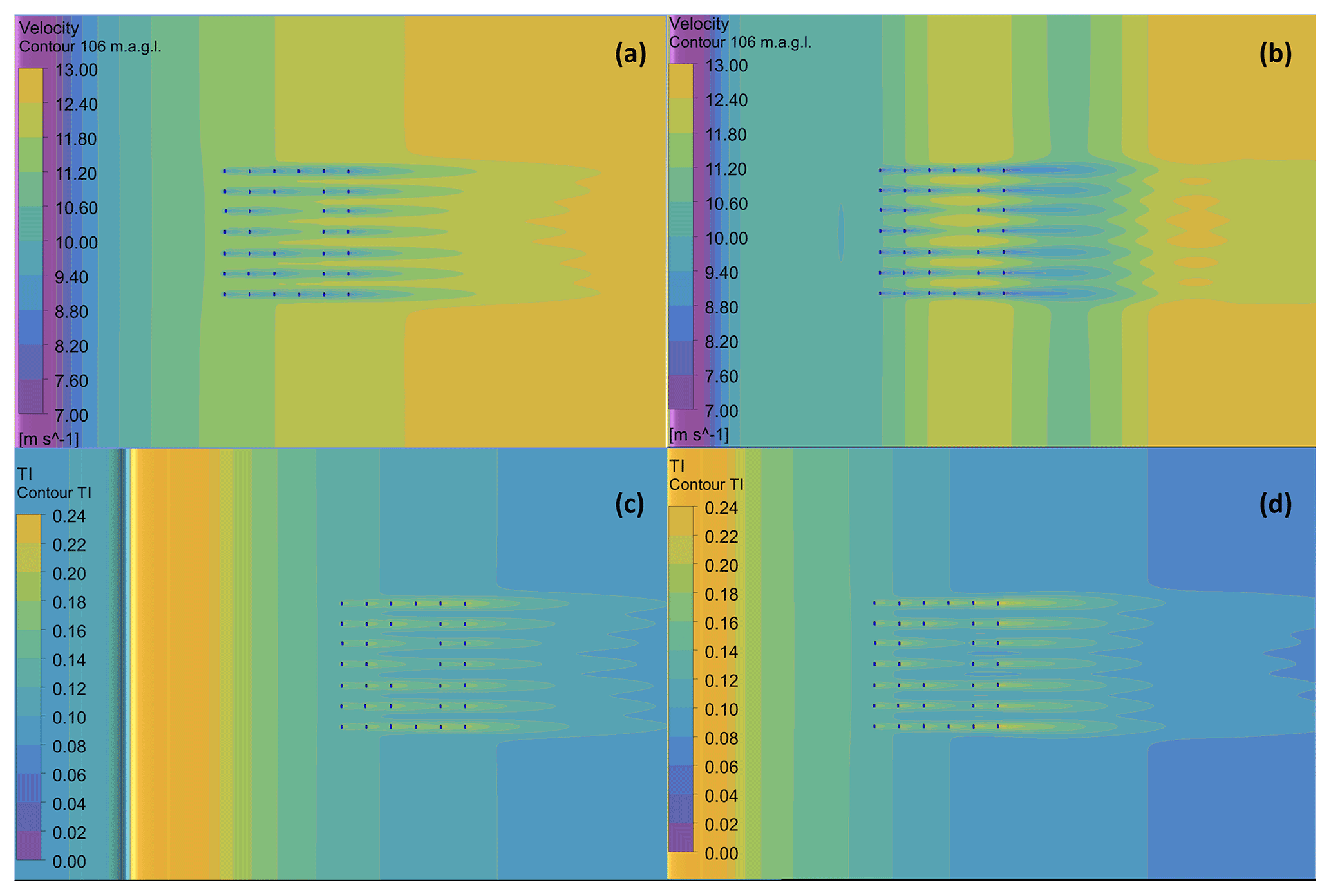
Figure C2WMR view from above in the CFD domain with colour contours of 106 m hub height wind speeds and TI for (a), (c) r0Nh-WMR and (b), (d) r7Nh-WMR, see legend for wind speeds.
The measurement and reanalysis data used in this paper are open source. ERA5 reanalysis data (Hersbach et al., 2023) are available at https://doi.org/10.24381/cds.bd0915c6. SAR 10 m wind field data are managed by DTU and available at https://doi.org/10.11583/DTU.19704883.v1 (Badger et al., 2022). The Ansys WindModeller simulation input files are available at https://github.com/squaroh/WES_TLW (last access: 9 July 2023; https://doi.org/10.5281/zenodo.8127654, Ollier, 2023).
SJO was responsible for the project conceptualization, data curation, formal analysis, investigation, methodology, project administration, coding, software, validation, data analysis and visualization, and writing and editing of the paper. SJW was responsible for project supervision including conceptualization, funding acquisition, methodology, paper review, and editing.
The contact author has declared that neither of the authors has any competing interests.
Publisher’s note: Copernicus Publications remains neutral with regard to jurisdictional claims in published maps and institutional affiliations.
This research was funded by a NERC-CASE PhD studentship with the ORE Catapult and undertaken at Loughborough University.
This research has been supported by the Natural Environment Research Council (grant no. NE/M009971/1).
This paper was edited by Johan Meyers and reviewed by Jovanka Nikolic and one anonymous referee.
Allaerts, D. and Meyers, J.: Boundary-layer development and gravity waves in conventionally neutral wind farms, J. Fluid Mech., 814, 95–130, https://doi.org/10.1017/jfm.2017.11, 2017a.
Allaerts, D. and Meyers, J.: Gravity Waves and Wind-Farm Efficiency in Neutral and Stable Conditions, Bound.-Lay. Meteorol., 166, 266–269, https://doi.org/10.1007/s10546-017-0307-5, 2017b.
Allaerts, D. and Meyers, J.: Sensitivity and feedback of wind-farm-induced gravity waves, J. Fluid Mech., 862, 990–1028, https://doi.org/10.1017/jfm.2018.969, 2019.
Allaerts, D., Broucke, S. Vanden, Van Lipzig, N., and Meyers, J.: Annual impact of wind-farm gravity waves on the Belgian-Dutch offshore wind-farm cluster, J. Phys.-Conf. Ser., 1037, 72006, https://doi.org/10.1088/1742-6596/1037/7/072006, 2018.
ANSYS Inc.: Ansys CFX-Solver Theory Guide, Release 2021 R2, Canonsburg, PA, p. 154, https://dl.cfdexperts.net/cfd_resources/Ansys_Documentation/CFX/Ansys_CFX-Solver_Theory_Guide.pdf (last access: 11 July 2023), 2021.
Argyle, P.: Computational fluid dynamics modelling of wind turbine wake losses in large offshore wind farms, incorporating atmospheric stability, PhD thesis, Loughborough University, https://repository.lboro.ac.uk/articles/thesis/Computational_fluid_dynamics_modelling_of_wind_turbine_wake_losses_in_large_offshore_wind_farms_incorporating_atmospheric_stability/9538733 (last access: 7 July 2021), 2014.
Badger, M., Karagali, I., and Cavar, D.: Offshore wind fields in near-real-time, Technical University of Denmark, DTU Data [data set], https://doi.org/10.11583/DTU.19704883.v1, 2022.
Chunchuzov, I., Vachon, P. W., and Li, X.: Analysis and Modeling of Atmospheric Gravity Waves Observed in RADARSAT SAR Images, Remote Sens. Environ., 74, 343–361, https://doi.org/10.1016/S0034-4257(00)00076-6, 2000.
Draxl, C., Worsnop, R. P., Xia, G., Pichugina, Y., Chand, D., Lundquist, J. K., Sharp, J., Wedam, G., Wilczak, J. M., and Berg, L. K.: Mountain waves can impact wind power generation, Wind Energ. Sci., 6, 45–60, https://doi.org/10.5194/wes-6-45-2021, 2021.
Durran, D. R. and Klemp, J. B.: A Compressible Model for the Simulation of Moist Mountain Waves, Mon. Weather Rev., 111, 2341–2361, https://doi.org/10.1175/1520-0493(1983)111<2341:ACMFTS>2.0.CO;2, 1983.
Gadde, S. N. and Stevens, R. J. A. M.: Effect of Coriolis force on a wind farm wake, J. Phys.-Conf. Ser., 1256, 012026, https://doi.org/10.1088/1742-6596/1256/1/012026, 2019.
Garratt, J. R.: Appendix 3, First., Cambridge atmospheric and space science series, Cambridge University Press, Cambridge, UK, ISBN 9780521477449, 1994.
Gossard, E. E. and Hooke, W. H.: Waves in the Atmosphere, Elsevier, New York, 456 pp., ISBN 0444411968, 1975.
Haupt, S. E., Berg, L. K., Decastro, A., Gagne, D. J., Jimenez, P., Juliano, T., Kosovic, B., Mirocha, J. D., Quon, E., Sauer, J., Allaerts, D., Churchfield, M. J., Draxl, C., Hawbecker, P., Jonko, A., Kaul, C. M., McCandless, T., Munoz-Esparza, D., Rai, R. K., and Shaw, W. J.: Report of the Atmosphere to Electrons Mesoscale-to-Microscale Coupling Project, Alexandria, Office of Scientific and Technical Information (OSTI), U.S. Department of Energy, https://doi.org/10.2172/1735568, 2019.
Hersbach, H., Bell, B., Berrisford, P., Biavati, G., Horányi, A., Muñoz Sabater, J., Nicolas, J., Peubey, C., Radu, R., Rozum, I., Schepers, D., Simmons, A., Soci, C., Dee, D., and Thépaut, J.-N.: ERA5 hourly data on pressure levels from 1940 to present, Copernicus Climate Change Service (C3S) Climate Data Store (CDS) [data set], https://doi.org/10.24381/cds.bd0915c6, 2023.
Hills, M. O. G. and Durran, D. R.: Nonstationary Trapped Lee Waves Generated by the Passage of an Isolated Jet, J. Atmos. Sci., 69, 3040–3059, https://doi.org/10.1175/JAS-D-12-047.1, 2012.
International Organization for Standardization: Standard Atmosphere, ISO 2533:1975, Geneva, Switzerland, https://www.iso.org/standard/7472.html (last access: 11 July 2023), 1975.
Jia, M., Yuan, J., Wang, C., Xia, H., Wu, Y., Zhao, L., Wei, T., Wu, J., Wang, L., Gu, S.-Y., Liu, L., Lu, D., Chen, R., Xue, X., and Dou, X.: Long-lived high-frequency gravity waves in the atmospheric boundary layer: observations and simulations, Atmos. Chem. Phys., 19, 15431–15446, https://doi.org/10.5194/acp-19-15431-2019, 2019.
Klemp, J. B. and Lilly, D. K.: Numerical Simulation of Hydrostatic Mountain Waves, J. Atmos. Sci., 35, 78–107, https://doi.org/10.1175/1520-0469(1978)035<0078:NSOHMW>2.0.CO;2, 1978.
Lanzilao, L. and Meyers, J.: Set-point optimization in wind farms to mitigate effects of flow blockage induced by atmospheric gravity waves, Wind Energ. Sci., 6, 247–271, https://doi.org/10.5194/wes-6-247-2021, 2021.
Li, L., Chan, P. W., Zhang, L., and Hu, F.: Numerical Simulation of a Lee Wave Case over Three-Dimensional Mountainous Terrain under Strong Wind Condition, Adv. Meteorol., 2013, 304321, https://doi.org/10.1155/2013/304321, 2013.
Li, X.: Atmospheric Vortex Streets and Gravity Waves, SAR Marine User’s Manual, 341–354 pp., https://www.sarusersmanual.com/ManualPDF/NOAASARManual_CH16_pg341-354.pdf (last access: 7 July 2023), 2004.
Li, X., Zheng, W., Yang, X., Zhang, J. A., Pichel, W. G., and Li, Z.: Coexistence of Atmospheric Gravity Waves and Boundary Layer Rolls Observed by SAR, J. Atmos. Sci., 70, 3448–3459, 2013.
Maas, O. and Raasch, S.: Wake properties and power output of very large wind farms for different meteorological conditions and turbine spacings: a large-eddy simulation case study for the German Bight, Wind Energ. Sci., 7, 715–739, https://doi.org/10.5194/wes-7-715-2022, 2022.
Montavon, C. A., Hui, S., Graham, J., Malins, D., Housley, P., Dahl, E., de Villierts, P., and Gribben, B.: Offshore Wind Accelerator: Wake Modelling Using CFD, in: European Wind Energy Association Conference and Exhibition, https://www.ewea.org/events/past-events-and-proceedings/ (last access: 10 August 2018), 2011.
Nappo, C. J.: Mountain Waves, in: International Geophysics, vol. 102, Academic Press, 57–85, https://doi.org/10.1016/B978-0-12-385223-6.00003-3, 2012.
Ollier, S.: Trapped lee wave interactions with an offshore wind farm, PhD thesis, Loughborough University, https://repository.lboro.ac.uk/articles/thesis/Trapped_lee_wave_interactions_with_an_offshore_wind_farm/21583917/1 (last access: 7 July 2023), 2022.
Ollier, S.: squaroh/WES_TLW: wes-2022-83 (v1.0.0), Zenodo [code] and [data set], https://doi.org/10.5281/zenodo.8127654, 2023.
Ollier, S. J., Watson, S. J., and Montavon, C.: Atmospheric gravity wave impacts on an offshore wind farm, IOP Conf. Ser. J. Phys., 1037, 072050, https://doi.org/10.1088/1742-6596/1037/7/072050, 2018.
Rasmussen, E. A. and Aakjær, P. D.: Two Polar Lows Affecting Denmark, 47, 326–338, https://doi.org/10.1002/j.1477-8696.1992.tb07196.x, 1992.
Romanova, N. N. and Yakushkin, I. G.: Internal gravity waves in the lower atmosphere and sources of their generation (review), Ocean. Phys. C/C, 31, 151–172, 1995.
Smith, R. B.: Gravity wave effects on wind farm efficiency, Wind Energy, 13, 449–458, https://doi.org/10.1002/we.366, 2010.
Thomson, R. E., Vachon, P. W., and Borstad, G. A.: Airborne synthetic aperture radar imagery of atmospheric gravity waves, J. Geophys. Res.-Ocean., 97, 14249–14257, https://doi.org/10.1029/92JC01178, 1992.
Vachon, P. W., Johannessen, O. M., and Johannessen, J. A.: An ERS 1 synthetic aperture radar image of atmospheric lee waves, J. Geophys. Res.-Ocean., 99, 22483–22490, https://doi.org/10.1029/94JC01392, 1994.
Vosper, S. B., Ross, A. N., Renfrew, I. A., Sheridan, P., Elvidge, A. D., and Grubišiæ, V.: Current Challenges in Orographic Flow Dynamics: Turbulent Exchange Due to Low-Level Gravity-Wave Processes, Atmos.-Basel, 9, 361, https://doi.org/10.3390/atmos9090361, 2018.
Warner, T. T.: Numerical Weather and Climate Prediction, Cambridge University Press, https://doi.org/10.1017/CBO9780511763243, 2010.
Wilczak, J. M., Stoelinga, M., Berg, L. K., Sharp, J., Draxl, C., McCaffrey, K., Banta, R. M., Bianco, L., Djalalova, I., Lundquist, J. K., Muradyan, P., Choukulkar, A., Leo, L., Bonin, T., Pichugina, Y., Eckman, R., Long, C. N., Lantz, K., Worsnop, R. P., Bickford, J., Bodini, N., Chand, D., Clifton, A., Cline, J., Cook, D. R., Fernando, H. J. S., Friedrich, K., Krishnamurthy, R., Marquis, M., McCaa, J., Olson, J. B., Otarola-Bustos, S., Scott, G., Shaw, W. J., Wharton, S., and White, A. B.: The Second Wind Forecast Improvement Project (WFIP2): Observational Field Campaign, B. Am. Meteorol. Soc., 100, 1701–1723, https://doi.org/10.1175/BAMS-D-18-0035.1, 2019.
Wu, K. L. and Porté-Agel, F.: Flow Adjustment Inside and Around Large Finite-Size Wind Farms, 10, 2164, https://doi.org/10.3390/en10122164, 2017.
Xia, G., Draxl, C., Raghavendra, A., and Lundquist, J. K.: Validating simulated mountain wave impacts on hub-height wind speed using SoDAR observations, Renew. Energ., 163, 2220–2230, https://doi.org/10.1016/j.renene.2020.10.127, 2021.
Xu, Q., Li, X., Bao, S., and Pietrafesa, L. J.: SAR Observation and Numerical Simulation of Mountain Lee Waves Near Kuril Islands Forced by an Extratropical Cyclone, IEEE T. Geosc. Remote, 54, 7157–7165, https://doi.org/10.1109/TGRS.2016.2596678, 2016.
When no flow prevails in the domain, the momentum conservation equation in the vertical is simplified to . The pressure profile used at the outflow is calculated by integrating this relationship from the ground to the top of the domain, using the prescribed profile for θin at the inflow and the reference potential temperature θ0. When using a pressure profile not satisfying the hydrostatic balance, the model generates flow acceleration or slow-down that can destabilize the solution.