the Creative Commons Attribution 4.0 License.
the Creative Commons Attribution 4.0 License.
 | 17 Aug 2023
Bayesian method for estimating Weibull parameters for wind resource assessment in a tropical region: a comparison between two-parameter and three-parameter Weibull distributions
Mohammad Golam Mostafa Khan
Mohammed Rafiuddin Ahmed
The two-parameter Weibull distribution has garnered much attention in the assessment of wind energy potential. The estimation of the shape and scale parameters of the distribution has brought forth a successful tool for the wind energy industry. However, it may be inappropriate to use the two-parameter Weibull distribution to assess energy at every location, especially at sites where low wind speeds are frequent, such as in tropical regions. In this work, a robust technique for wind resource assessment using a Bayesian approach for estimating Weibull parameters is first proposed. Secondly, the wind resource assessment techniques using a two-parameter Weibull distribution and a three-parameter Weibull distribution, which is a generalized form of two-parameter Weibull distribution, are compared. Simulation studies confirm that the Bayesian approach seems a more robust technique for accurate estimation of Weibull parameters. The research is conducted using data from seven sites in the tropical region from 1∘ N of the Equator to 21∘ S of the Equator. Results reveal that a three-parameter Weibull distribution with a non-zero shift parameter is a better fit for the wind data with a higher percentage of low wind speeds (0–1 m s−1) and low skewness. However, wind data with a smaller percentage of low wind speeds and high skewness showed better results with a two-parameter distribution that is a special case of the three-parameter Weibull distribution with a zero shift parameter. The proposed distribution can be incorporated into commercial software like WAsP to improve the accuracy of wind resource assessments. The results also demonstrate that the proposed Bayesian approach and application of a three-parameter Weibull distribution are extremely useful for accurate estimation of wind power density.
- Article
(5638 KB) - Full-text XML
- BibTeX
- EndNote


Wind energy has now become one of the world's fastest-growing sources of energy. It is an inexhaustible source of energy with increasing utilization all around the world. Growing climate change concerns have prompted many developed and developing countries to implement policies that reduce their reliance on non-renewable sources and instead utilize renewable sources such as wind, hydro and solar energies (Renner et al., 2022; IEA, 2021). However, developing countries encounter several challenges in generating sustainable wind energy. There is a need for reliable wind data and proper assessments of a country's wind energy potential before initiating energy generation projects that would help them meet the sustainable development goals set by the United Nations.
While climate change is being experienced globally, some regions are being affected more than the others. Pacific islands countries (PICs), particularly those in the warmer tropical region, are more susceptible to its effects. The contribution of the PICs to the current global greenhouse gas emissions is below 0.03 %; yet they are among the first to be affected by climate change. It is projected that the people of PICs will be among the first who will need to adapt to climate change or be required to relocate from or abandon their traditional homeland. Some islands are already facing the impacts of climate change on their communities, infrastructure, water supply, coastal and forest ecosystems, fisheries, agriculture, and human health. Island states and territories such as Kiribati, the Marshall Islands, Tokelau and Tuvalu are the immediate victims of this phenomenon due to rising sea levels. Knowledge of the effects of climate change on PICs should act as a driving force behind the commitment to decrease greenhouse gas emissions. The PICs, which currently depend heavily on imported fossil fuels and their by-products, need to become more energy efficient and self-reliant (Weir, 2018). PICs are among the countries with the lowest access to electricity, and their prices of electricity are among the highest in the world due to their heavy reliance on high-cost diesel-based generation. Energy security and low-cost energy are becoming increasingly important within the region, which require increasing investments in renewable energy technologies. PICs are also among the countries most vulnerable to natural disasters (Robinson, 2020). The energy sector can be highly vulnerable to such events, which requires adequate attention to these issues in the design of energy production and distribution infrastructure. This can only be achieved by adopting resilient renewable energy policies. Most of the countries in the region have their national sustainable development plans to achieve the United Nations' sustainable development goals (SDGs); for example, the country of the Cook Islands aims to have 100 % renewable power generation in the near future and Fiji is committed to reducing 30 % of its national greenhouse gas emissions and achieving 99 % renewable energy generation by 2030 (MOE, 2017).
However, a lack of reliable and accurate wind resource data acts as a barrier to a clean-energy future in the PICs, especially in the smaller developing islands (Michalena et al., 2018). So far, wind resource assessment has received only limited attention in the PICs, and there is a need for further wind data collection and analysis and accurate wind energy potential assessment. The World Bank provides support to PICs through the Sustainable Energy Industry Development Project (SEIDP). In various phases of renewable energy resource mapping, it supports countries in carrying out assessments of solar and wind potential. The objectives of this component are to enhance awareness and knowledge of the potential for renewable technologies (solar and wind) among governments, power utilities and the private sector and to provide governments with a spatial planning framework to guide investments in the renewable energy sector (PPA, 2015).
The utilization of wind energy is slowly increasing in PICs such as New Caledonia, Fiji, Vanuatu, the Cook Islands and Samoa with the installation of wind farms. However, there have been few to no attempts to establish wind power in many of these countries. The University of the South Pacific installed towers of 34 m height, named Integrated Renewable Energy Resource Assessment Systems (IRERASs), in Kiribati, Nauru, Niue, Tuvalu, Tokelau, Samoa, Tonga, Fiji, Vanuatu, the Solomon Islands and the Cook Islands to collect data on wind and solar energy resources (Gosai, 2014).
The Weibull distribution has now become a widely accepted model in determining the potential of wind energy (Indhumathy et al., 2014). Wind energy professionals in different parts of the world have widely employed Weibull distributions in the statistical analyses of wind characteristics and for estimating wind power density (Corotis et al., 1978). The Weibull shape parameter defines the width of wind speed distribution. A higher shape parameter indicates that the distribution is narrower and the peak value is higher. The Weibull scale parameter controls the abscissa scale of the data distribution plot (Chang, 2011). Thus, the Weibull distribution function is comprehensively used for analysing the wind power potential at a site.
Past researchers found the two-parameter Weibull distribution to be a useful and practical tool for wind energy estimation. The advantages of two-parameter Weibull distribution include its flexibility, simplicity in parameter estimation and convenience for conducting goodness-of-fit tests on these parameters as well as its dependence on only two parameters that can be expressed in closed form. The present authors studied a number of methods for finding the Weibull parameters (shape factor and scale factor) for a number of sites: Kadavu (Kutty et al., 2019), Vanuatu (Singh et al., 2019) and the Cook Islands (Singh et al., 2022).
However, some authors have suggested that the two-parameter (2-p) Weibull distribution is not suited for all wind regimes encountered in nature such as regimes with a high percentage of low wind speeds and bimodal distributions. Therefore, its usage cannot be generalized. To minimize errors, a suitable probability density function must be carefully selected for different wind regimes. Carta et al. (2009), Sukkiramathi and Seshaiah (2020), and Patlakas et al. (2017) emphasized the importance of studying low wind speeds, stating that this information can be included in risk assessment. Leahy and Mckeogh (2013) studied the persistence of low-wind-speed conditions and their implications for the variability in wind power.
Tuller and Brett (1984) proposed a three-parameter Weibull function for wind data analysis and found that it showed better fitness and flexibility than the two-parameter Weibull function. Recently, some authors have utilized the three-parameter Weibull distribution and found that it has more flexibility with improved fitness than the two-parameter Weibull distribution in wind energy assessments. Wais (2017) compared the two- and three-parameter Weibull distributions to find the most appropriate distribution of wind speed. The results revealed that methods other than the three-parameter Weibull distribution cannot account for cases where the frequency of low wind speed is higher. The author compared the wind speeds for three different sites and found that the three-parameter Weibull distribution performed the best when there was a greater frequency of lower wind speeds. Sukkiramathi and Seshaiah (2020) and Wang et al. (2022) also utilized the three-parameter Weibull distribution for analysing wind power potential. However, to date, only limited research has been carried out on wind data analysis using the three-parameter Weibull distribution.
Furthermore, many estimation methods have been proposed for estimating Weibull parameters. Among these, maximum likelihood estimation (MLE), a popular frequentist technique, has been widely used for estimating the parameters (Teimouri and Gupta, 2013). Recently, the Bayesian estimation approach has received a lot of attention from many researchers. Among them are Ibrahim and Mohammed (2011), who considered the Bayesian survival estimator for Weibull distribution with censored data. Many authors, including Hossain and Zimmer (2003) and Pandey et al. (2011), conducted comparative studies on the estimation of the Weibull parameters using complete and censored samples, and Lye et al. (1993) determined the Bayes estimation for the extreme-value reliability function. Guure et al. (2012) examined the performance of MLE and Bayesian methods for estimating the two-parameter Weibull failure time distribution. However, the use of the Bayesian technique for modelling wind data and analysing wind power potential was not explored in their work.
The present work is aimed at comparing the two-parameter and three-parameter Weibull distributions to fit wind speed data more accurately at seven locations in the tropical region, where wind speeds are generally lower. Development of a novel approach using the Bayesian method for estimating the Weibull parameters is also a part of this work. The results from the Bayesian technique are compared with those of the traditional MLE method to determine a more accurate evaluation method of wind speed characteristics.
Wind speed data from seven different sites in the tropical region were used in the present work, as shown in Table 1.
Table 1Details of wind data collection sites. Data were collected at seven sites in the tropical region from the locations 1∘ N of the Equator to 21∘ S of the Equator in five countries during the period February 2012 to December 2019.
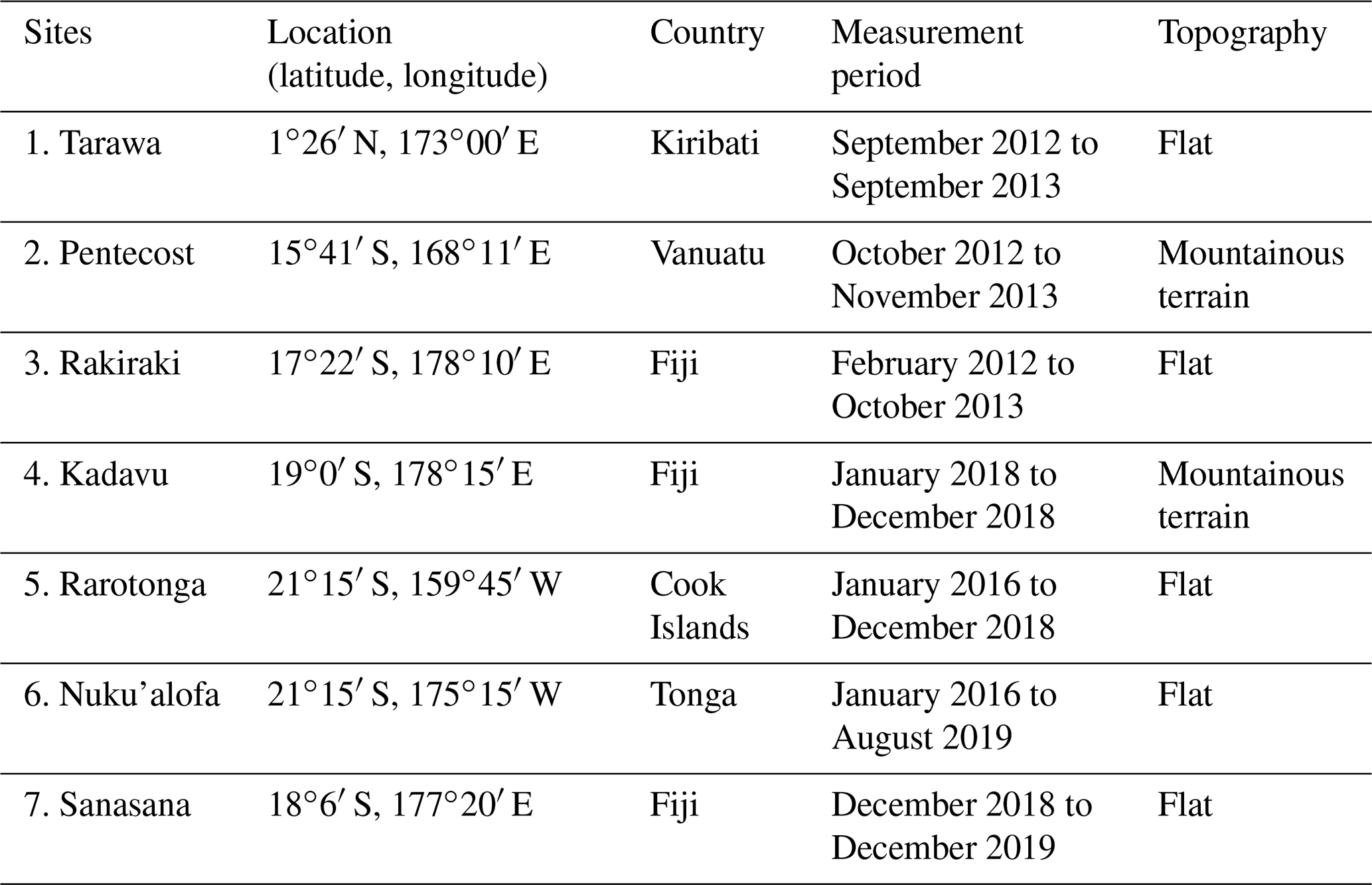
For sites 1, 2 and 3, data were obtained from measurements using 34 m tall towers with the help of sensors described in Table 2. The NRG Systems towers, named Integrated Renewable Energy Resource Assessment Systems (IRERASs), with a height of 34 m were used. NRG Systems SymphoniePLUS3 was the data logger used and was connected to seven different sensors installed on the tower. The sensors measured wind speed, temperature, pressure, rainfall, solar insolation, humidity and wind direction. The data were either collected from the SD card in person or sent via the GSM-based network to a data bank located at the Japan-Pacific ICT Centre of the University of the South Pacific at the Laucala Campus, Fiji. The anemometers (serial numbers 179500189054-57, 179500189089-90) have an accuracy of 0.1 m s−1 and a range of 0.4 to 96 m s−1. The wind vane is placed at 30 m above ground level (a.g.l.). The data were recorded in a time-series format in an RWD file and were later transferred to a Microsoft Excel sheet. The wind speed data were recorded continuously at an interval of 10 min with a three-cup anemometer – two at heights of 34 m a.g.l. and one at 20 m a.g.l. For sites 4, 5 and 6, satellite data were downloaded; land data from ERA5-Land were used in the present work (reference: https://cds.climate.copernicus.eu/, last access: 18 February 2021). ERA5 is the fifth-generation ECMWF reanalysis for the global climate and weather for the past 4 to 7 decades. Reanalysis combines model data with observations from across the world into a globally complete and consistent dataset using the laws of physics. This principle, called data assimilation, is based on the method used by numerical weather prediction centres: after a certain number of hours (12 h at ECMWF), a previous forecast is combined with newly available observations in an optimal way to produce a new best estimate of the state of the atmosphere, called analysis, from which an updated, improved forecast is issued. Reanalysis works in the same way but at reduced resolution to allow for the provision of a dataset spanning back several decades. Reanalysis does not have the constraint of issuing timely forecasts, so there is more time to collect observations and, when going further back in time, to allow for the ingestion of improved versions of the original observations, which all benefit the quality of the reanalysis product. For site 7, an NRG Systems tower, similar to the ones used for sites 1, 2 and 3 but 50 m high, was installed; it has anemometers at 50, 40 and 30 m a.g.l.
Table 2Specifications of the relevant measurement sensors (Aukitino et al., 2017). The sensors were mounted on a 34 m NRG Systems tower. The data were averaged and recorded every 10 min.
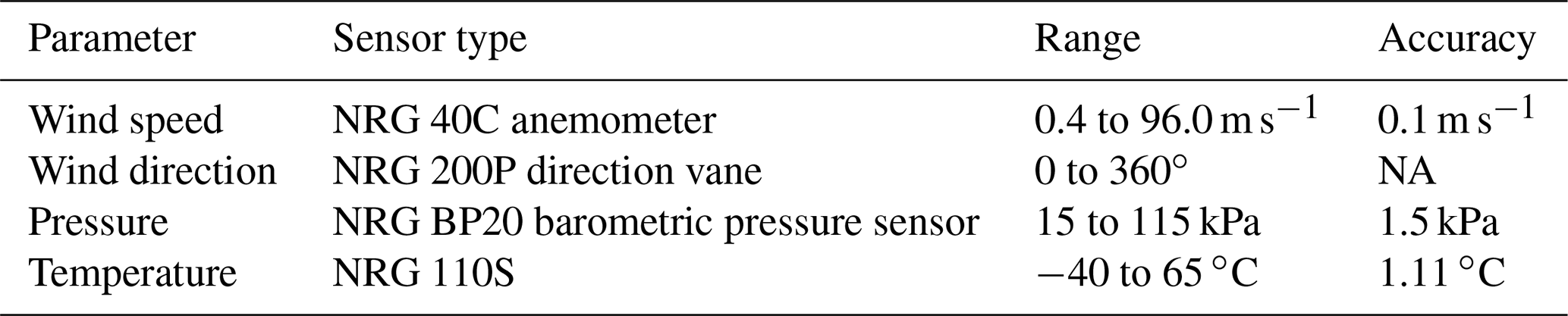
NA: not available.
For the measured values, some uncertainties were taken into account such as calibration errors, the terrain of the site that was used, the dynamic over-speeding, the error introduced due to wind shear and the inflow angle (Jain, 2016). The measurements in the present work were performed close to the shoreline on flat terrain. The flow was in the horizontal plane, resulting in a lower uncertainty level. The calibration report for the anemometers used in the present work showed a maximum uncertainty of 0.6 % for a wind speed range of 4–7 m s−1, which reduced at higher wind speeds. The overall uncertainty in the estimation of wind speed is obtained by taking all the above uncertainties into account (Jain, 2016) and using the relation in Eq. (1):
where εi is each component of uncertainty and N is the number of components of uncertainty. The uncertainties were estimated at a 95 % confidence level. As per the International Electrotechnical Commission (IEC) standard IEC 61400-12-1 (IEC, 2017), the uncertainty in the measurements was estimated to be approximately 1.74 %.
Assessment of wind power energy at a site requires knowledge of the appropriate probability distribution of the site's wind speed, as the estimation of wind energy depends on its accuracy.
3.1 Two-parameter Weibull distribution
The two-parameter Weibull probability density functions (PDFs) and the cumulative distribution function (CDF) for wind speed, U, are given, respectively, by
and
where f(U) is the probability of observing the wind speed, k is the shape parameter and A is the scale parameter (m s−1) of the distribution. The parameter k indicates the wind potential and what peak the distribution can reach. Its value ranges between 1 and 3. A lower k value signifies highly variable winds, while constant winds are characterized by a larger k. The parameter A denotes how windy the site under study is, and it takes a value proportional to the mean wind speed (Manwell et al., 2010; Sukkiramathi and Seshaiah, 2020).
3.2 Three-parameter Weibull distribution
The three-parameter Weibull PDF and the CDF for wind speed are given, respectively, by
and
where f(U) is the probability of observing the wind speed, k is the shape parameter, A is the scale parameter (m s−1), and θ is the shift or location parameter (m s−1) of the distribution. If θ=0, f(U) and F(U) become the PDF and CDF, respectively, of a two-parameter Weibull distribution.
As the name implies, the shift parameter, θ, shifts the distribution along the abscissa. When θ=0, the distribution starts at U=0 or at the origin, whereas if θ>0, the distribution starts at the location θ to the right of the origin. If θ<0, the distribution starts with the location parameter θ to the left of the origin. For the distribution of wind speed, θ provides an estimate of the location of the distribution (Tuller and Brett, 1984; Wais, 2017). However, when θ<0, one may encounter the issue that the integral of the standard probability distribution (Eq. 4) over non-negative wind speeds becomes considerably less than 1. In such cases, when there is significant loss in the integral value, a truncated version of the three-parameter Weibull distribution supporting positive wind speed only with a finite probability of calm wind speed (U=0) may be used, as given by
where fcalm is a postulated probability of calm situations given by
and δ(U) is Kronecker's delta function.
To estimate the Weibull parameters, we propose a Bayesian approach and compare its performance with a popular frequentist approach, the maximum likelihood estimation (MLE) method.
4.1 The maximum likelihood estimation (MLE) method
4.1.1 Two-parameter distribution
MLE is the most popular technique for deriving estimators (Aukitino et al., 2017; Casella and Berger, 2020; Chaurasiya et al., 2018) If U1, …, Un comprises the wind speed values with the Weibull density function given in Eq. (2), the shape parameter (k) and scale parameter (A) are the values that maximize the likelihood function . Then, solving and gives the equation of MLE of the scale parameter A as
Finally, Eq. (9) is used for estimating the shape parameter (k) as
which may be solved to get an estimate of k using the Newton–Raphson method or any other numerical procedure because Eq. (9) does not have a closed-form solution. When the value of k is obtained, the value of A can be found using Eq. (8).
4.1.2 Three-parameter distribution
The likelihood function L for estimating the parameters is given by . Then, solving , and gives the equations of MLE of the parameters as shown in Eqs. (10)–(12):
There is no closed-form solution of the equations, but Eqs. (10)–(12), which are non-linear, may be solved by applying some optimization techniques such as the Newton–Raphson method or other numerical procedures (Teimouri and Gupta, 2013; Lawless, 2003).
4.1.3 Evaluation of MLE methods
To determine the best model, we can compare the fit of the two MLE methods using different measures of the goodness of fit (Luceño, 2008; Cousineau and Allan, 2015; Ramachandran and Tsokos, 2021). The most used criteria are as follows.
The log-likelihood (log-like) method
If a PDF is fitted on the wind speed data and is the estimated parameter of the distribution, then the log likelihood for the goodness of fit is obtained by the following equation:
where Ui is the ith observed wind speed and n is the number of observations in the dataset. A higher log-likelihood value indicates a better fit.
Akaike information criterion (AIC)
If k is the number of distribution parameters to estimate, AIC is obtained using Eq. (14):
A lower value of AIC indicates that the model fits the data better. Compared to the log-likelihood method, this criterion takes into consideration the parsimony of the model as it includes a penalty term that increases the number of parameters.
Bayesian information criterion (BIC)
This criterion is obtained using Eq. (15):
Similarly to AIC, a lower value of BIC indicates that the model fits the data better. However, BIC provides a stronger penalty than AIC for additional parameters.
Kolmogorov–Smirnov (KS) test
The Kolmogorov–Smirnov (KS) test is also used to check the adequacy of a given theoretical distribution for a given set of wind speed data. The KS test computes the maximum difference between the predicted and observed distribution, and the test statistic D is given by
where is the ith predicted cumulative probability from the theoretical CDF and Fi is the empirical probability of the ith observed wind speed.
Anderson–Darling (AD) test
For a finite data sample, the Anderson–Darling (AD) test statistic A2 is defined by
where .
4.2 The Bayesian method
A classical frequentist approach such as MLE has certain drawbacks. Most of its properties hold only for large sample sizes, and it requires a symmetric form of sample distribution. The Bayesian approach, however, is free from such limitations. Moreover, Bayesian simulation tools provide an exact method of inference even if the sample size is very small. Thus, in real-life situations where the sample size may be small, Bayesian methods seem to be more suitable over frequentist methods if prior information about the parameters is available.
In this paper, a Bayesian inference approach for modelling of wind speed data is proposed. In the Bayesian paradigm, data and prior information about the parameters are combined together to make an inference about the parameters of interest.
The most influential contribution of the Bayesian approach is its modification of the likelihood function into a posterior distribution – a valid probability distribution defined by the classic Bayes' rule. The posterior distribution of wind speed is expressed as
where p(η|U) is the posterior distribution of wind speed, p(η) is the prior distribution of unknown parameters , p(U|η) is the likelihood of wind speed data and . The denominator of Eq. (18), p(U), normalizes the posterior distribution, p(η|U). Since it is independent of U, it is often convenient to write the posterior distribution as
i.e. the posterior distribution of the parameters is proportional to the likelihood function times the prior distribution of parameters. While fitting wind speed data, a non-informative uniform prior distribution is used, as very little prior knowledge about its model parameters is available. In Bayesian computations, a sample of the joint posterior distribution is obtained by using Gibbs sampler to simulate a sample from a Markov chain Monte Carlo (MCMC) method. Then, we can calculate the desired values of the posterior.
In this paper, the software JAGS is used to fit the model. The R package
R2jags is used to summarize the posterior inference, which is discussed in
more detail in Sect. 4.2.1.
4.2.1 Bayesian fitting of Weibull distribution with JAGS
JAGS, an acronym for “Just Another Gibbs Sampler” (Plummer,
2003), accepts a model string written in an R-like syntax that compiles and
generates MCMC samples from the model using Gibbs sampling. It is open-source software written in C using GNU compilers and packaging
tools – freely available at http://mcmc-jags.sourceforge.net/ (last access: 21 January 2022).
R packages such as R2jags or rjags enable running JAGS models within R on
Windows machines for the summarization of posterior inference.
In the present work, JAGS models for the Bayesian fit of wind speed with two-
and three-parameter Weibull distributions are developed and MCMC data are
generated. In MCMC simulations, the Gibbs sampler with the JAGS models is
run for 10 000 iterations using the jags function in the R2jags package
(Su and Yajima, 2020). Then, the posterior estimates of parameters
are obtained by performing the Gibbs sampler iterations and using a burn-in period of 1000 to attain convergence with five thinning intervals and three chains and a sample size of 1800 per chain. The model specifications to
perform the Bayesian fit, as well as the jags function and its arguments, are
presented in Appendix A. The computational time for the 2-p Weibull method
is approximately 24 min, while that for the three-parameter (3-p) Weibull method is
approximately 34 min compared to about 1 and 2 min,
respectively, for the MLE method. It should, however, be noted that a direct
comparison of the computational time would not be appropriate as the
Bayesian method is a simulation-based technique which takes a longer time than
the standard software-based MLE technique.
4.2.2 Evaluation of Bayesian models
The standard likelihood, AIC and BIC statistics, discussed in Sect. 4.1.3, are not relevant while evaluating Bayesian methods such as MCMC. Instead, Spiegelhalter et al. (2002) suggested that the deviance information criterion (DIC) should be used to compare models. DIC is a generalization of AIC that is based on deviance statistics:
where h(U) is a standardizing function of the data. DIC is then defined as
where is the posterior expectation of deviance and pD is the effective number of parameters that captures the complexity of a model. A smaller value of DIC indicates a better-fitting model.
When the wind speed (U) of a site and the frequency distribution f(U) are known, the wind power density can be estimated. If ρ is the density of air, D is the turbine rotor diameter and is the rotor cross-sectional area, then the probability of wind power for a given velocity U is obtained by
Then, the expected wind power (P) is estimated by
Substituting Eqs. (22), (2) and (4) into Eq. (23), the expected total wind power densities for two-parameter and three-parameter Weibull distributions, respectively, are determined by
and
The efficiency and performance of MLE and Bayesian methods for estimating two- and three-parameter Weibull distributions were determined using different goodness-of-fit and error measures such as the coefficient of determination (R2), root mean square error (RMSE), coefficient of efficiency (Rocha et al., 2012), mean absolute error (MAE) and mean absolute percentage error (MAPE). Arithmetically, these are computed as follows (Kidmo et al., 2015; Aukitino et al., 2017; Azad et al., 2014).
Coefficient of determination (R2)
R2 is a statistical measure that gives some information about the goodness of fit of a model, that is, how much the variance of the observed data is explained by the fitted model. It is defined as
where n is the number of observations, Ui is the ith actual data, is the ith predicted data with the Weibull distribution and is the mean of actual data. A higher R2 value indicates a better fit, and R2= 1 indicates that the regression predictions perfectly fit the data.
Root mean square error (RMSE)
RMSE determines the deviation of the predicted values of wind speed from the observed values and is obtained by
A smaller RMSE value normally indicates accurate modelling. The calculated RMSE value approaches zero as the difference between the observed and predicted values becomes smaller (Indhumathy et al., 2014).
Coefficient of efficiency (COE)
COE quantifies the ratio of difference between predicted wind speed and the mean wind speed to the difference between actual values and the average of wind speeds. A higher COE value indicates a good fit to the data. It is expressed as
Mean absolute error (MAE)
MAE is a measure of the absolute difference between predicted and actual values. A smaller value of MAE indicates higher accuracy. MAE is mathematically expressed as
Mean absolute percentage error (MAPE)
MAPE is a comparative measure, indicating the error as a percentage of the actual data that help accurately predict the forecasting method. Like MAE, a lower value of MAPE indicates better accuracy. It is mathematically expressed as
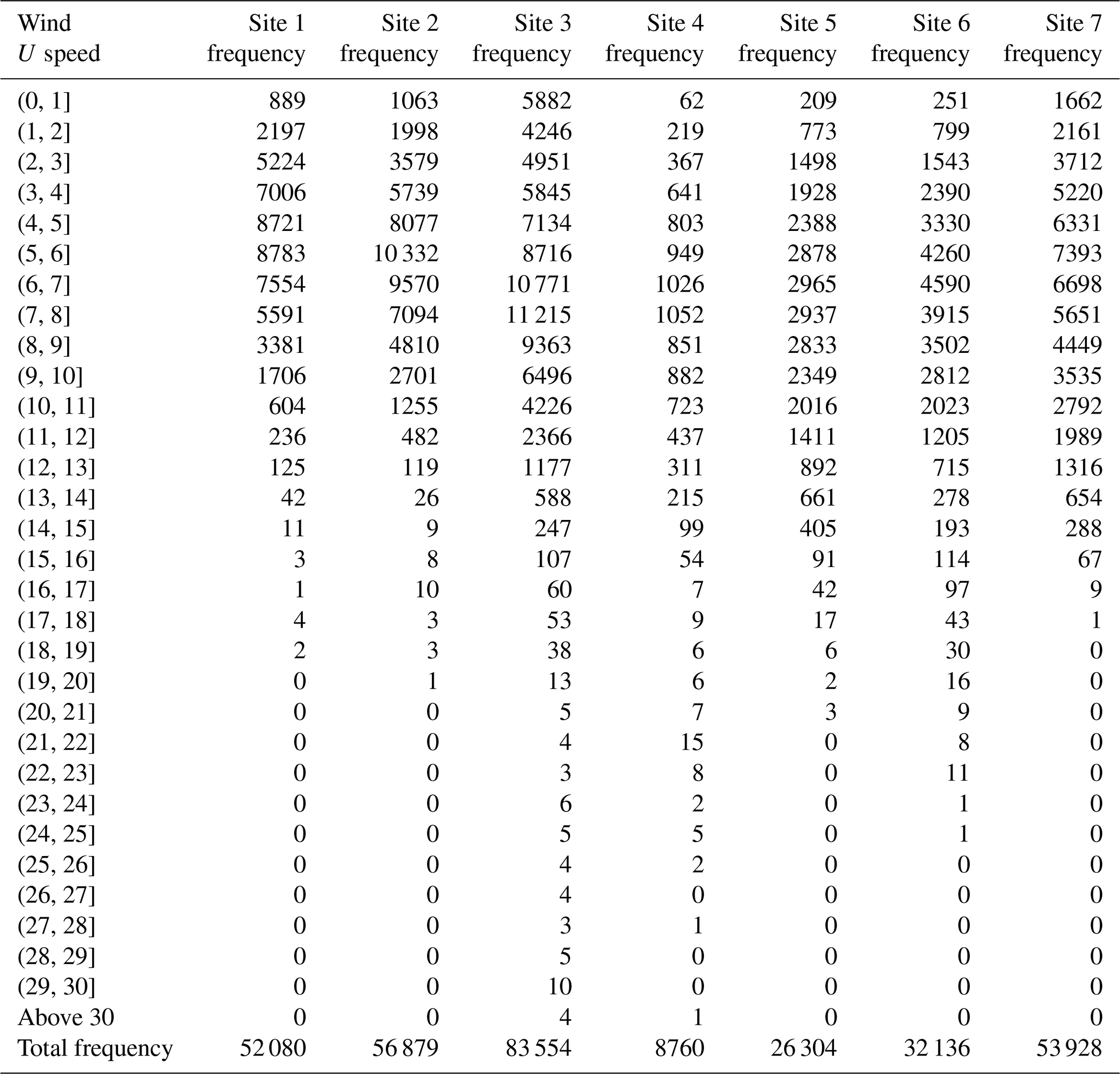
In this section, the results of fitting of two-parameter (2-p) and three-parameter (3-p) Weibull distributions are presented. Further, the results for the application of MLE and the proposed Bayesian approach for estimating the parameters, as described in Sects. 3 and 4, are also presented. To accomplish this, wind speed data at seven different sites were collected as mentioned in Sect. 2. Table 3 provides wind speed distributions at these sites. The table shows that the range of speeds varies at different sites. The lowest range of wind speed was observed at site 1 (0–19 m s−1), and the highest range was found at site 3 (0–34 m s−1). Some sites tend to have more low to null wind speeds (0–1 m s−1).
Table 3Frequency distributions of wind speeds at the seven different sites. The frequencies are counted at wind speed intervals of 0–1, 1–2 m s−1 and so on.
Both the 2-p and 3-p Weibull distributions were fitted to the recorded wind speed data, and the parameters in the distributions were estimated using the MLE and the Bayesian methods. In the MLE method, the goodness of fit with 2-p and 3-p Weibull distributions is evaluated using the statistical measures AIC, BIC, AD, KS and log-like. Table 4 presents the estimated values of the parameters of 2-p and 3-p Weibull distributions and the values of the various statistical measures determined by the MLE at the seven sites. The values highlighted in bold in this table and the subsequent tables indicate which distribution performs better.
Table 4Estimated values of the parameters obtained with the MLE method for both 2-p and 3-p Weibull distributions at all the seven sites. The statistical measures AIC, BIC, AD, KS and log-like are also listed for the comparison of two fitted distributions according to the MLE method.
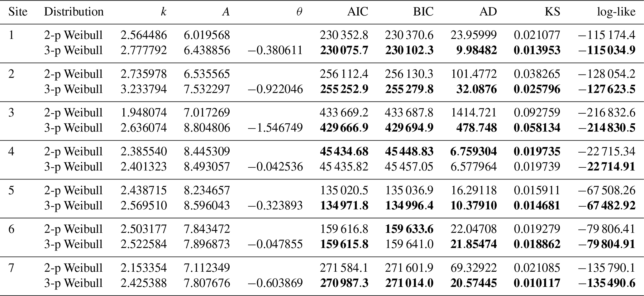
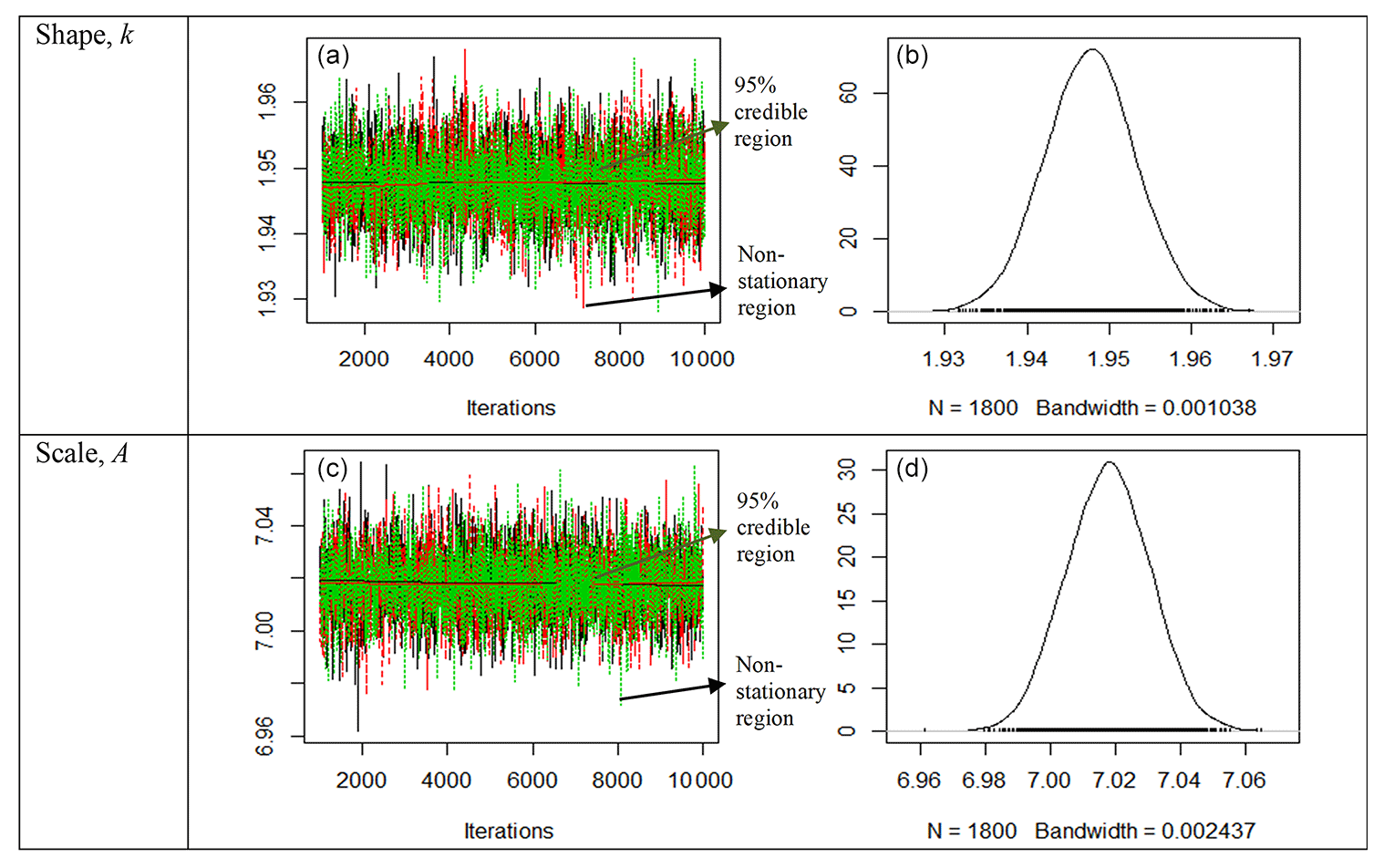
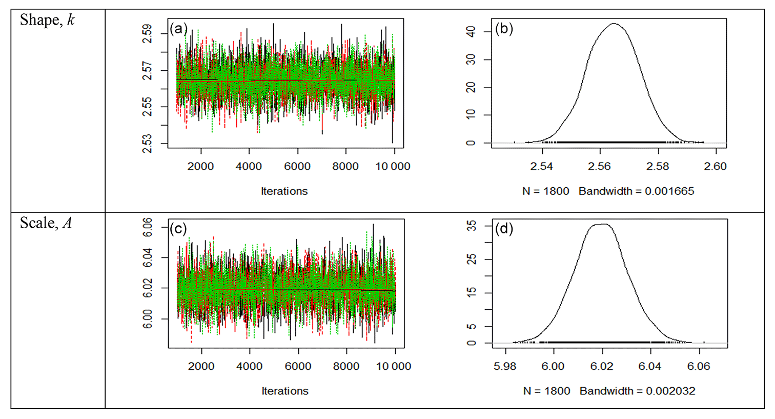
Figure 1Trace plots (a, c) and posterior density plots (b, d) for the two parameters of the 2-p Weibull distribution for site 3. The trace plots show a fat-hairy-caterpillar appearance, which is indicative of a random scatter around the stable mean of the shape parameter at k=1.947640 and the scale parameter A=7.017671. The density plots also display smooth curves of the simulated values of both the parameters. Thus, the plots clearly indicate the convergence of the simulations of the Bayesian estimates.
In Bayesian estimates, uniform prior distributions of the parameters were used to fit wind data. Firstly, a sample of the joint posterior distribution by simulating a sample from MCMC methods using a Gibbs sampler as discussed in Sect. 4.2.1 is obtained. Finally, DIC is obtained to evaluate the Bayesian parameters of the Weibull distributions. Table 5 presents the estimated mean values of the parameters with the standard deviation (SD) of both two- and three-parameter Weibull distributions for all the sites. The 95 % credible region (lower limit 2.5 % and upper limit 97.5 %) for each of the parameters and the model evaluation statistic DIC values are also presented.
Table 5Estimated mean values of the parameters with SD obtained using the Bayesian method for both 2-p and 3-p Weibull distributions at all the seven sites. The 95 % credible region (lower limit 2.5 % and upper limit 97.5 %) and the statistical measure DIC are also listed for the comparison of two fitted distributions according to the Bayesian method.
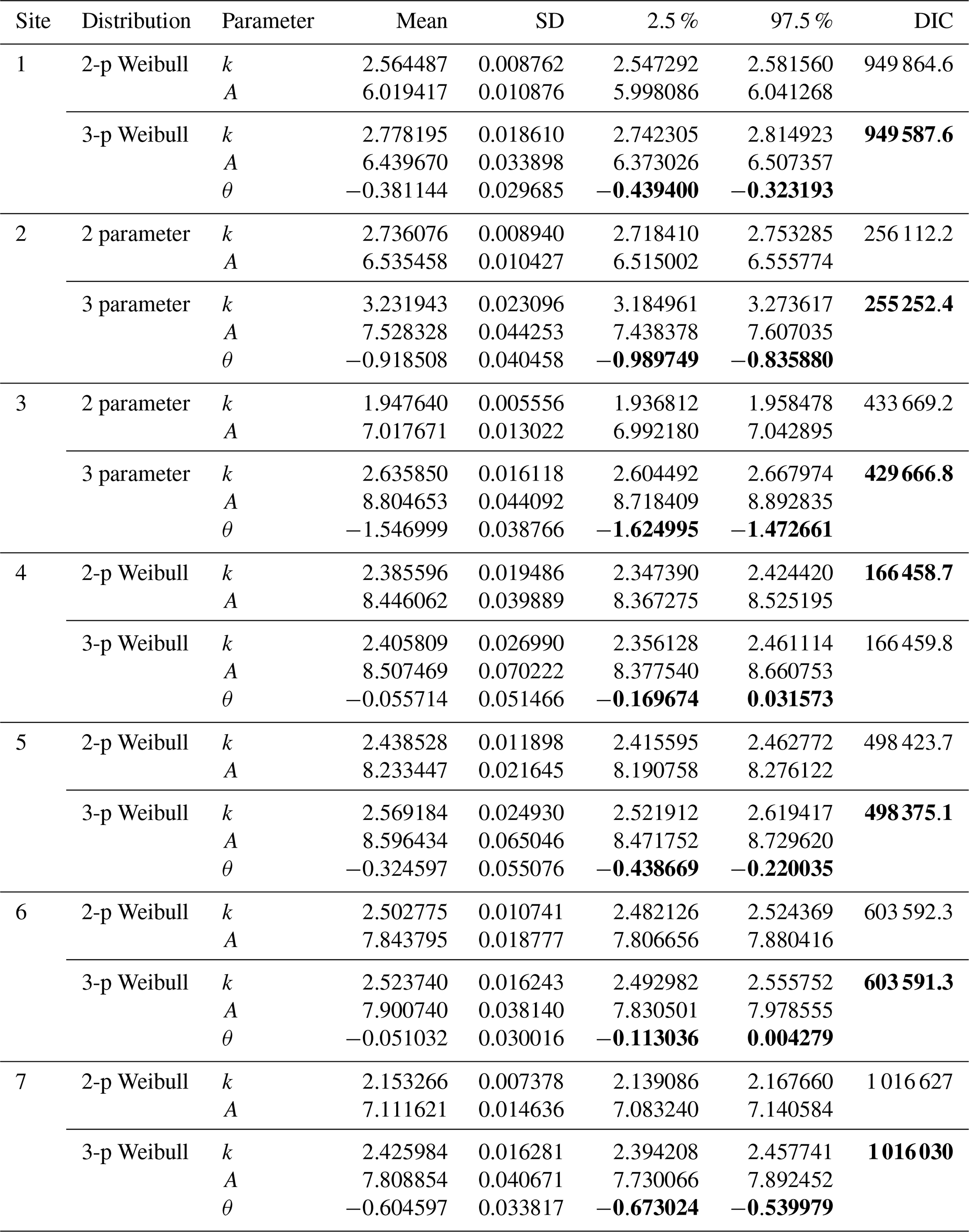
The goodness-of-fit criteria and the summary statistics presented in Tables 4 and 5 indicate that the 3-p Weibull distribution fits better than the 2-p Weibull distribution for wind speed at sites 1, 2, 3, 5 and 7 as all the goodness-of-fit measures (AIC, BIC, AD, KS and log-like) are smaller in the MLE estimate and DIC is also smaller in the Bayesian estimate. Moreover, as shown in Table 5, the marginal posterior means of the shift parameter θ are −0.381144, −0.918508, −1.546999, −0.324597 and −0.604597. The 95 % credible regions of this parameter as shown in columns 2.5 % and 97.5 % clearly indicate that the 3-p Weibull distribution is more appropriate at these sites as the value of its shift parameter is non-zero (i.e. θ≠0). Sites with a negative location parameter have also been reported in previous publications, for example in Wais (2017).
However, for site 4, both MLE results in Tables 4 and 5 indicate that the 2-p Weibull distribution fits better than the 3-p Weibull distribution at this site as AIC, BIC and KS are smaller in the MLE estimate and DIC is smaller in the Bayesian estimate. Although the marginal posterior mean of θ of the 3-p Weibull distribution is −0.055714, its 95 % credible region (−0.169674, 0.031573) indicates that the value of its shift parameter is zero (i.e. θ= 0). This implies that the 3-p Weibull distribution reduces to the 2-p Weibull distribution, indicating that the 2-p Weibull distribution is more appropriate at this site.
In contrast, at site 6, the results show a lack of significant difference between the 2-p and 3-p Weibull distributions while fitting wind speeds, as all MLE and Bayesian estimates are similar in their numerical values. Also, the 95 % credible region indicates that θ=0 in the Bayesian estimate, which indicates the 2-p Weibull distribution may be a better distribution at this site as the 3-p Weibull distribution reduces to the 2-p Weibull distribution. It should be noted that the 3-p Weibull distribution is a generalized form of the 2-p distribution, and when θ=0, it becomes the 2-p distribution. Thus, the 2-p distribution can be seen as a special case of the 3-p distribution.
Finally, since the Bayesian estimation is a simulation-based iterative procedure, the convergence of the model is diagnosed by the visual inspections using trace and posterior density plots. Samples of such plots obtained for the parameters of 2-p Weibull and 3-p Weibull distributions from the Bayesian simulations are presented in Figs. 1–4 for sites 3 and 4. Samples of some more plots for sites 1, 5 and 6 are also presented in Figs. B1–B6 in Appendix B.
In Fig. 1, trace plots (left) of the 2-p Weibull distribution for site 3 show a “fat-hairy-caterpillar” appearance, which is indicative of a random scatter around the stable mean of the shape parameter k=1.947640 within the 95 % credible region (1.936812, 1.958478) and the scale parameter A=7.017671 within the 95 % credible region (6.992180, 7.042895). Outside of this, the region is marked as a non-stationary region. For the subsequent plots , the region around the stable mean is also the 95 % credible region and the region outside of it is also the non-stationary region. The repeated simulated values from the three chains are shown in this figure and the two subsequent figures. The density plots (right) also display smooth curves of these simulated values for both the parameters. Thus, the plots clearly indicate the convergence of the simulations of the Bayesian estimates presented in Table 5.
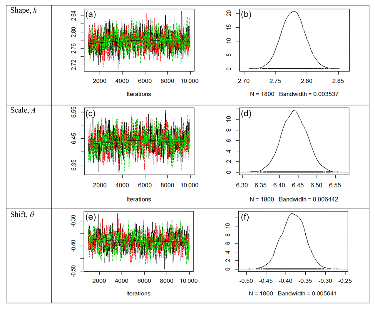
In Fig. 2, the trace plots (left) of the 3-p Weibull distribution also show a fat-hairy-caterpillar appearance, which indicates a random scatter around the stable mean of the shape parameter k=2.635850 within the 95 % credible region (2.604492, 2.667974) and the scale parameter A=8.804653 within the 95 % credible region (8.718409, 8.892835). The shift parameter shows a random scatter around the stable mean of within the 95 % credible region (−1.624995, −1.472661), which is far away from zero, and it reveals the appropriateness of using the 3-p Weibull distribution. The density plots (right) also display smooth curves of these simulated values for all the parameters. Thus, the plots clearly indicate the convergence of the simulations of Bayesian estimates presented in Table 5.
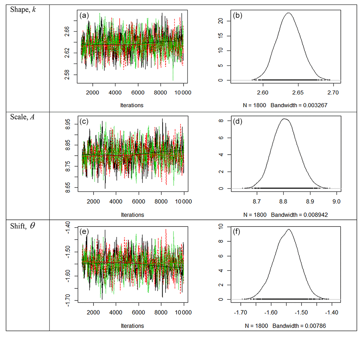
Figure 2Trace plots (a, c, e) and posterior density plots (b, d, f) for the three parameters of the 3-p Weibull distribution for site 3. The trace plots (a, c, e) of the 3-p Weibull distribution also show a fat-hairy-caterpillar appearance, which indicates a random scatter around the stable mean of the shape parameter k=2.635850 within the 95 % credible region (2.604492, 2.667974) and the scale parameter A=8.804653 within the 95 % credible region (8.718409, 8.892835). The shift parameter shows a random scatter around the stable mean of within the 95 % credible region (−1.624995, −1.472661), which is far away from zero, and it reveals the appropriateness of using the 3-p Weibull distribution. The density plots (b, d, f) also display smooth curves of these simulated values for all the parameters. Thus, the plots clearly indicate the convergence of the simulations of Bayesian estimates presented in Table 5.
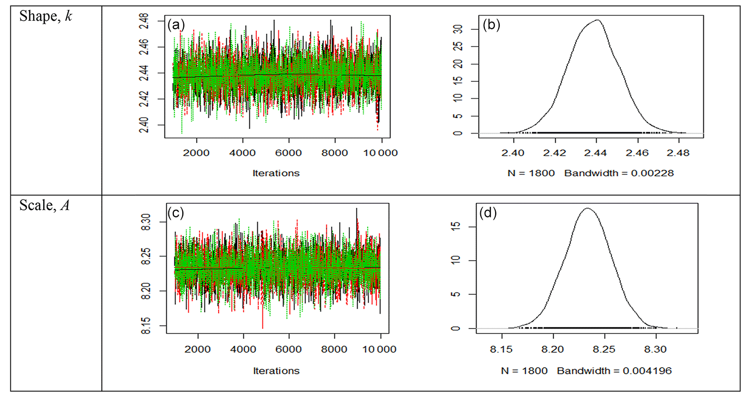
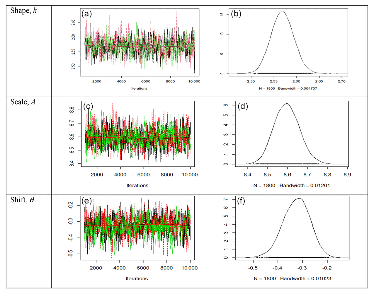
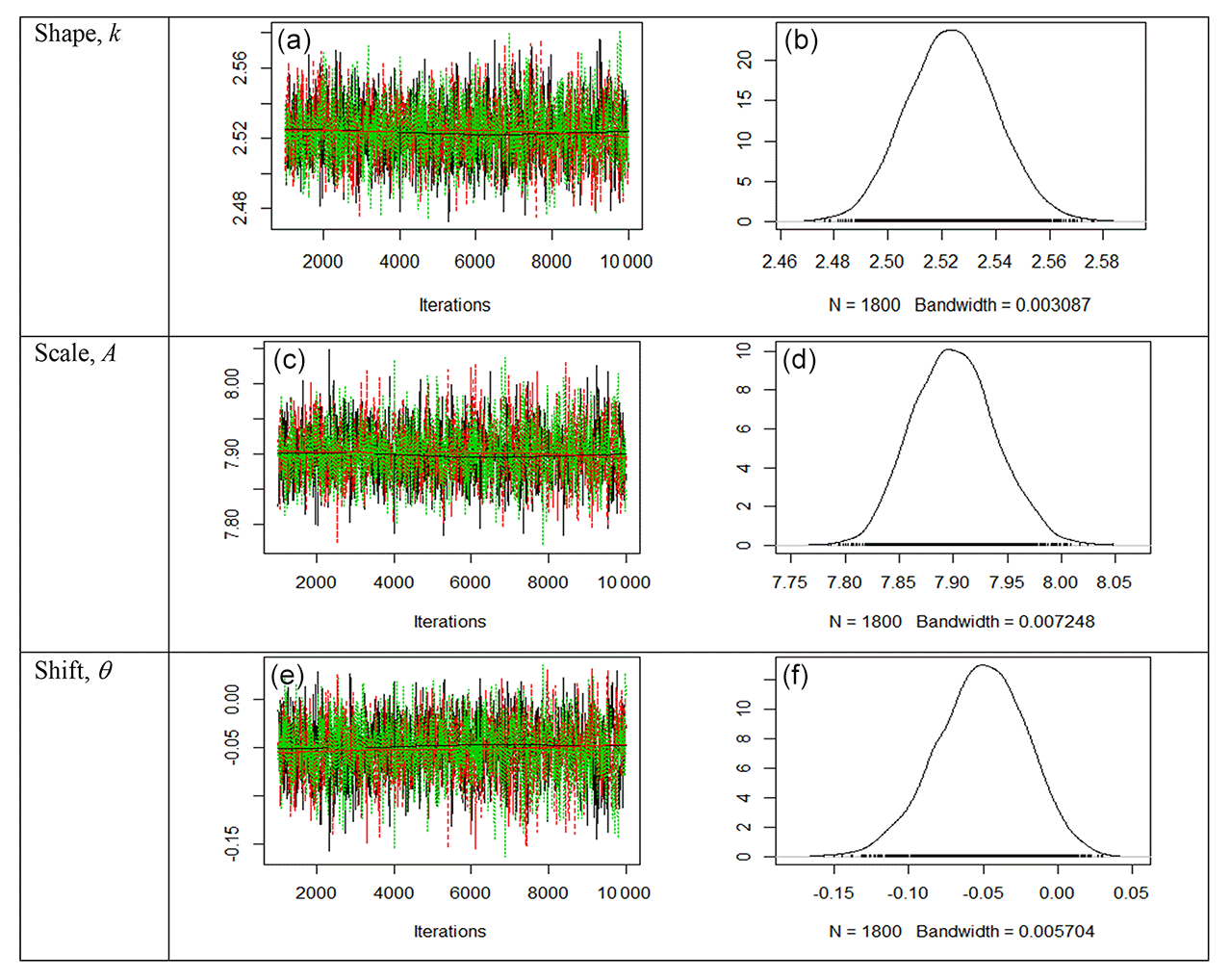
Similarly, from Figs. 3–4, the trace plots (left) for site 4 indicate a random scatter around the stable mean of the shape parameter k and the scale parameter A, which are within their 95 % credible regions for both 2-p Weibull and 3-p Weibull distributions. The shift parameter in Fig. 4 also shows a random scatter around the stable mean of within the 95 % credible region (−0.169674, 0.031573), which includes zero, and it reveals the appropriateness of using the 2-p Weibull distribution. The density plots (right) also display smooth curves of these simulated values for all the parameters. Thus, the plots clearly indicate the convergence of the simulations of Bayesian estimates presented in Table 5.
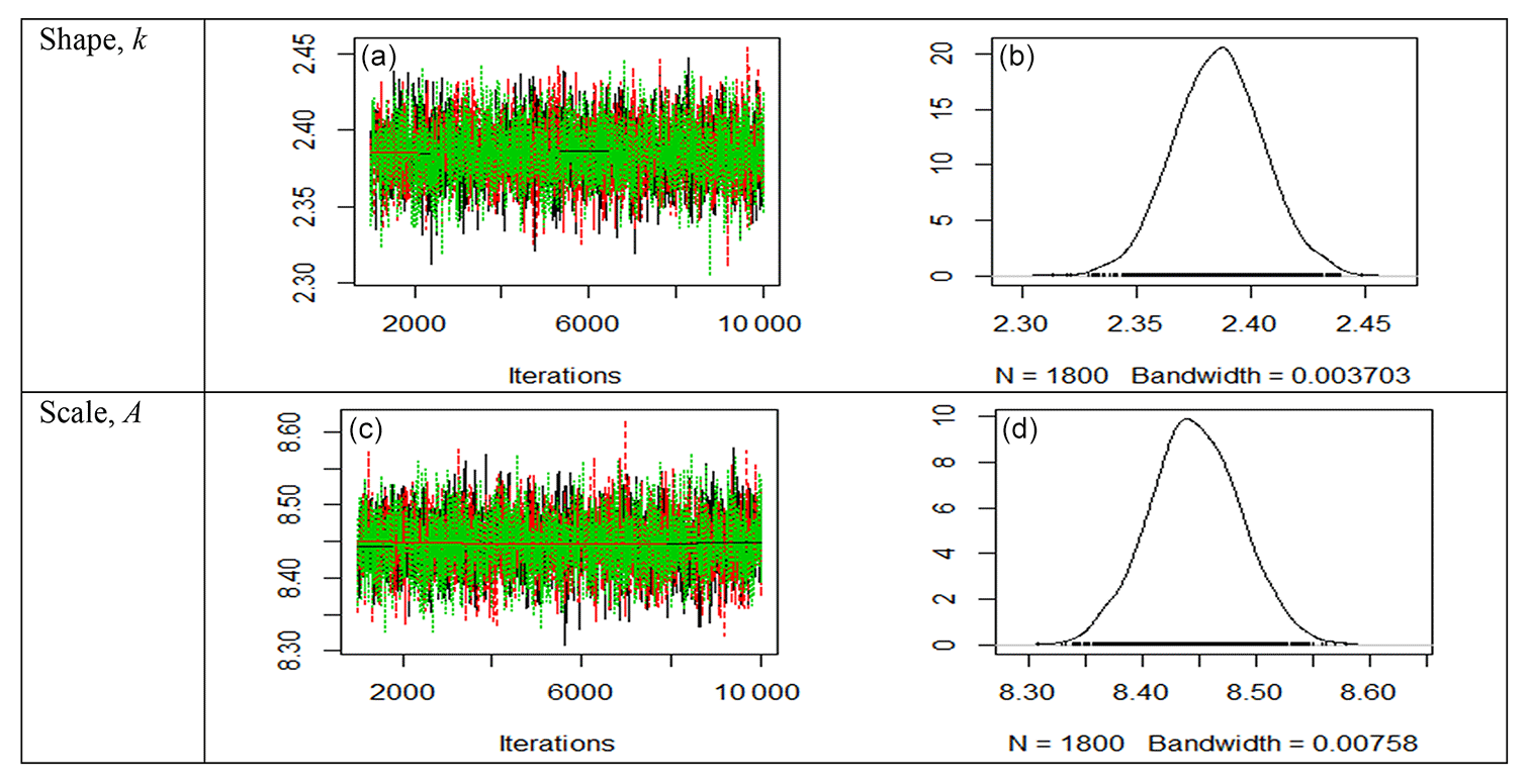
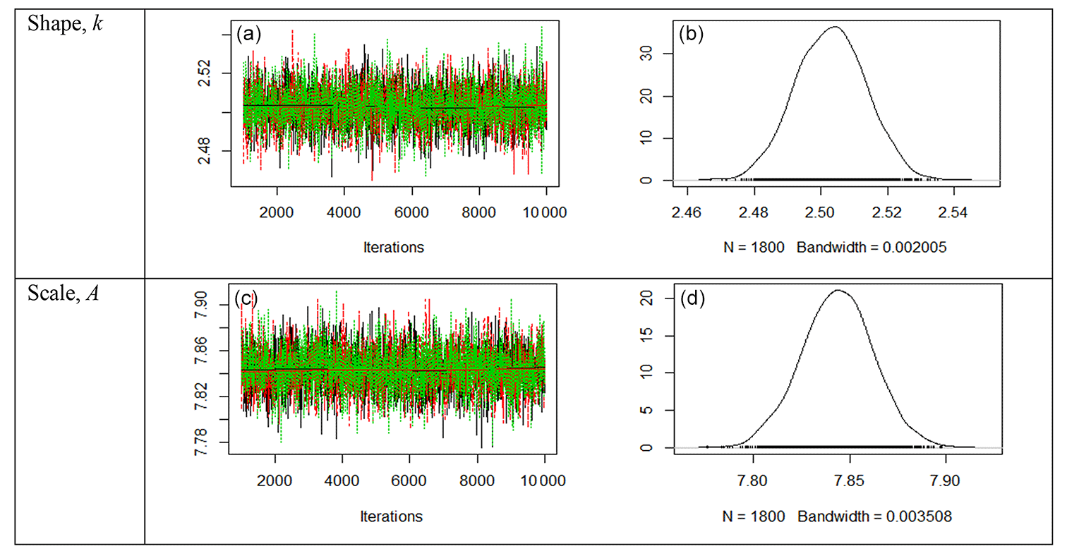
Figure 3Trace plots (a, c) and posterior density plots (b, d) for the two parameters of the 2-p Weibull distribution for site 4. The trace plots indicate a random scatter around the stable mean of the shape parameter k and the scale parameter A, which are within their 95 % credible regions. The density plots also display smooth curves of the simulated values for all the parameters. Thus, the plots clearly indicate the convergence of the simulations of Bayesian estimates presented in Table 5.
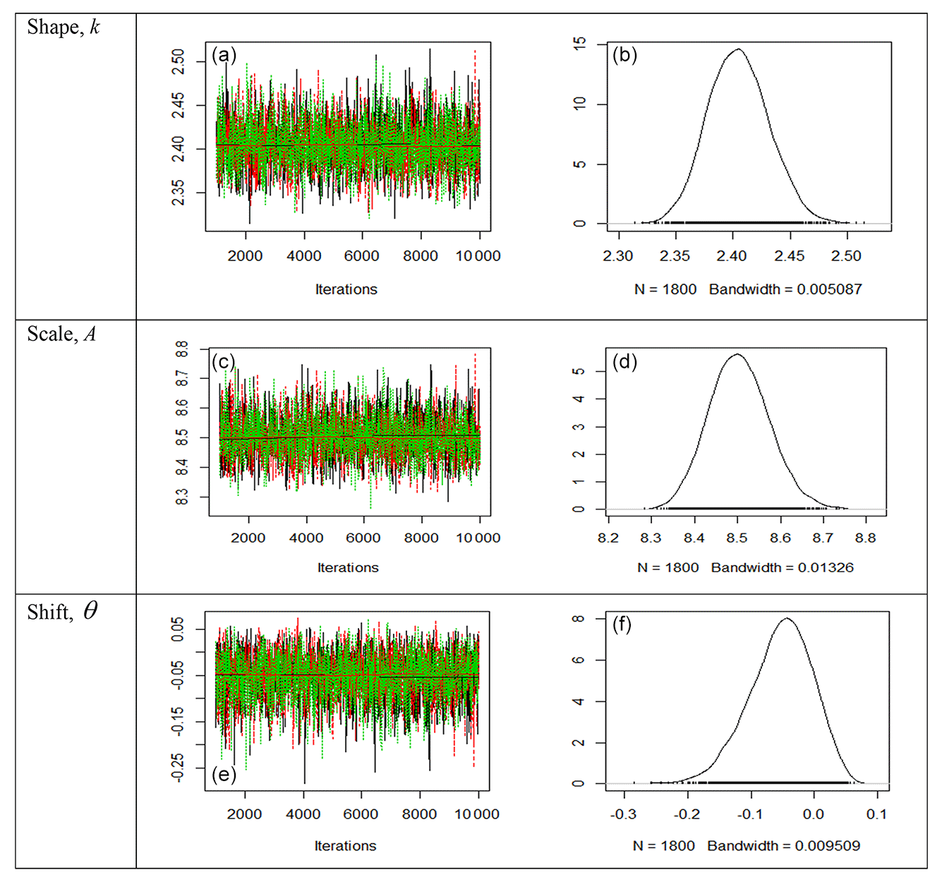
Figure 4Trace plots (a, c, e) and posterior density plots (b, d, f) for the two parameters of the 3-p Weibull distribution for site 4. The trace plots indicate a random scatter around the stable mean of the shape parameter k and the scale parameter A, which are within their 95 % credible regions. The shift parameter in the figure also shows a random scatter around the stable mean of within the 95 % credible region (−0.169674, 0.031573), which includes zero, and it reveals the appropriateness of using the 2-p Weibull distribution. The density plots (b, d, f) also display smooth curves of these simulated values for all the parameters. Thus, the plots clearly indicate the convergence of the simulations of Bayesian estimates presented in Table 5.
In Sect. 7, the results for the goodness of fit for the wind speed distributions at seven different sites were presented. Results showed that the 3-p Weibull distribution is a better fit for wind speeds at all the sites investigated, except sites 4 and 6, in the tropical region. The 2-p Weibull distribution may be a better fit for wind speed data at sites 4 and 6 because the shift parameter θ in the 3-p Weibull distribution was found to be zero as detected in the Bayesian estimate. As discussed earlier, the 2-p Weibull distribution can be considered a special case of the 3-p Weibull distribution.
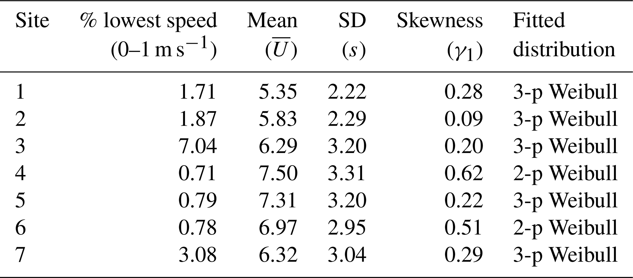
In this section, results of further investigations carried out to explain the difference between the performance of the two distributions are presented and discussed. Referring to the percentage of the lowest wind speeds (0–1 m s−1) presented in Table 6, the results clearly show that the wind speed distributions of the sites that have a high percentage (0.79 %–7.04 %) of lower (or closer to null) wind speeds (sites 1, 2, 3, 5 and 7) perfectly fit the 3-p Weibull distribution. The shift parameter in the simulations is also found to be significant; i.e. θ≠0 for these sites. On the other hand, the 2-p Weibull distribution was a better fit for wind speed distributions at sites 4 and 6, where the percentage of low wind speeds was smaller (<0.78 %). Similar findings were reported by Wais (2017).
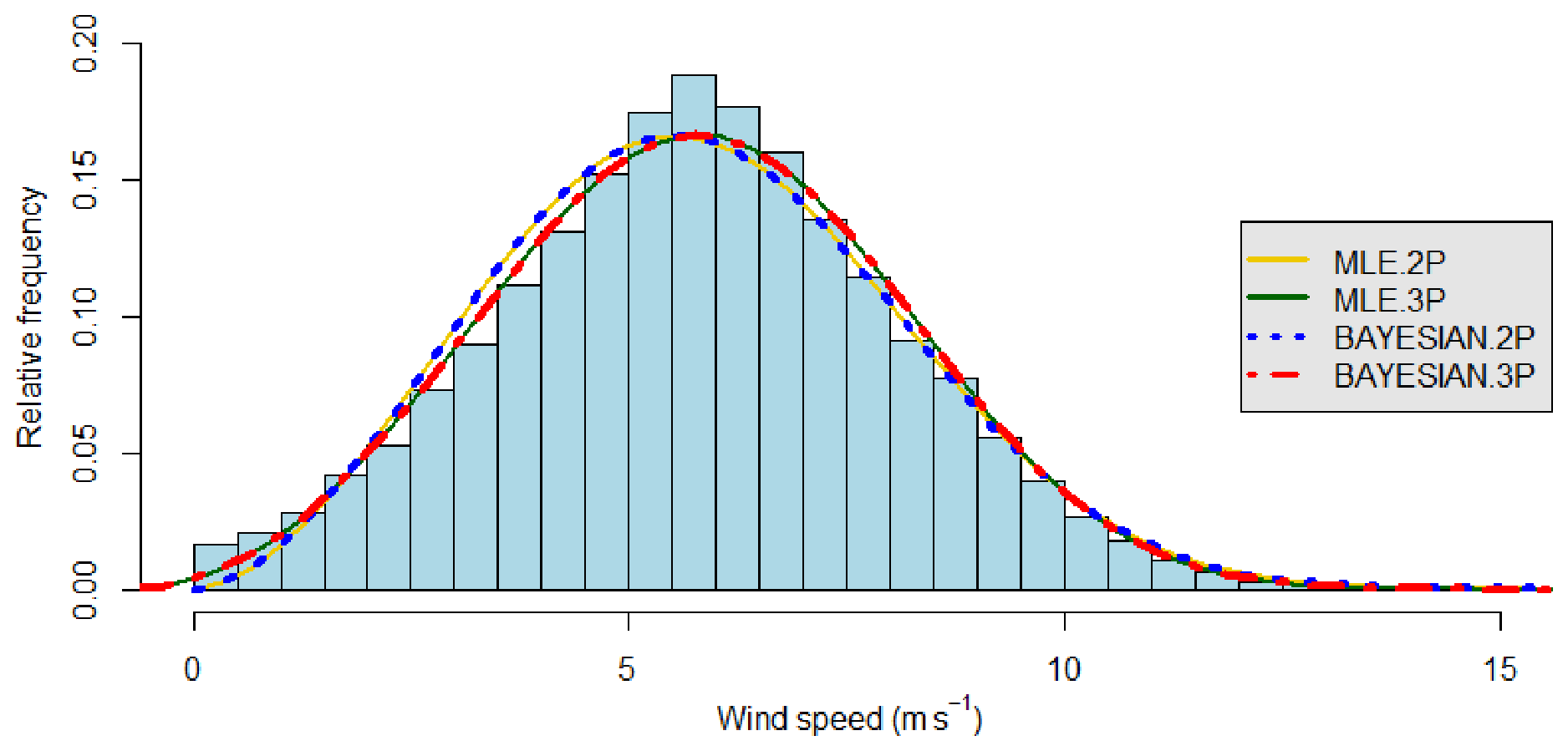
Figure 5The 2-p and 3-p Weibull curves by four methods and histogram of the observed wind speeds at site 2. The histogram shows that the wind speed distribution is almost symmetric. The mean wind speed is 5.83 m s−1, which is close to the centre, and the standard deviation of the site's wind speed is the lowest with a very small skewness compared to the other sites. The percentage of lowest wind speeds (0–1 m s−1) is found to be relatively high at this site as compared to others. From the distribution curves, it can also be seen that the Bayesian 3-p distribution fits the histogram well – it is evident from Table 7 that R2 is the highest – while the RMSE, MAE and MAPE values are the lowest for the Bayesian 3-p method at this site.
Moreover, histograms presented in Figs. 5–8 as a sample of such plots for wind speed distributions at sites 2, 3, 5 and 7 show different shapes, indicating a variation in skewness. Thus, another reason for fitting a better distribution is the skewness of the wind speed distribution. The skewness (γ1) is a measure of the asymmetry of the wind speed distribution about its mean, which is defined for a sample of n values as
where s is the standard deviation and is the third central moment. A normal distribution is symmetrical and has γ1= 0. If γ1 is negative, the distribution is left skewed, whereas a positive γ1 indicates a right-skewed distribution. Since the Weibull distribution is a right-skewed one, γ1 is expected to be positive.
Table 6 presents the mean (), standard deviation (s) and skewness (γ1) of the wind speed data at each site. It shows that the wind speed distributions of sites 4 and 6 have higher skewness compared to sites 1, 2, 3, 5 and 7.
Table 6Percentage of lowest wind speeds at different sites. The mean, SD and skewness of the wind speed data at each site are also presented. The last column gives the best-fitting Weibull distribution determined at each site.
Thus, the results reveal that the 3-p Weibull distribution is a better fit for wind speed data with both greater frequency of low wind speeds (0–1 m s−1) and low skewness compared to a 2-p Weibull distribution. The Bayesian analysis also confirms that the wind speed data with a smaller percentage of low speeds fitted better as the 2-p Weibull distribution than the 3-p Weibull distribution as its shift parameter θ was found to be zero.
To reiterate, this research is aimed at comparing the goodness of fit of both 2-p and 3-p Weibull distributions and at comparing the performance of frequentist MLE and Bayesian methods for the estimation of Weibull parameters. Therefore, a comparison study of the four methods is conducted by
-
fitting of the 2-p Weibull distribution with an MLE estimate – MLE.2p
-
fitting of the 3-p Weibull distribution with an MLE estimate – MLE.3p
-
fitting of the 2-p Weibull distribution with a Bayesian estimate – BAYESIAN.2p
-
fitting of the 3-p Weibull distribution with a Bayesian estimate – BAYESIAN.3p.
The wind speed bins and the Weibull distribution curves obtained using these four methods are illustrated in Figs. 5–8 as samples from four sites. The figures show that for all the sites, except sites 4 and 6, the 3-p Weibull distributions are closer to the histograms than the 2-p Weibull distributions. The Weibull distribution curves of Bayesian estimates are also closer to the histograms than MLE estimates. Thus, the 3-p Weibull distribution is a better fit for the wind speed data compared to the 2-p Weibull distribution (Aukitino et al., 2017).
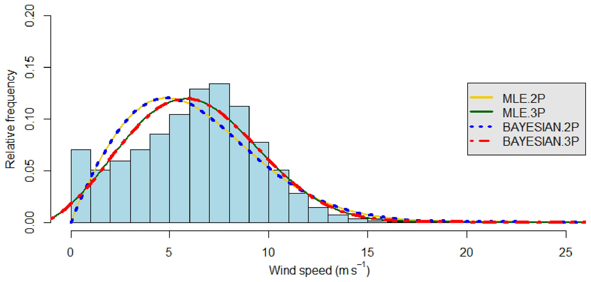
Figure 6The 2-p and 3-p Weibull curves by four methods and histogram of the observed wind speeds at site 3. The figure shows a non-symmetric distribution of wind speeds with the highest percentage of wind speeds of 0–1 m s−1 and a higher standard deviation. The mean wind speed for this site is 6.29 m s−1. Due to the high occurrence of very low wind speeds, the Bayesian 3-p Weibull distribution is a better fit for this case. However, due to the peculiar distribution of wind speeds at this site, the Weibull distribution does not fit the histogram perfectly like at site 2. It is clear from Table 7 that R2 is the highest, while the RMSE, MAE and MAPE values are the lowest for the Bayesian 3-p method for this site.
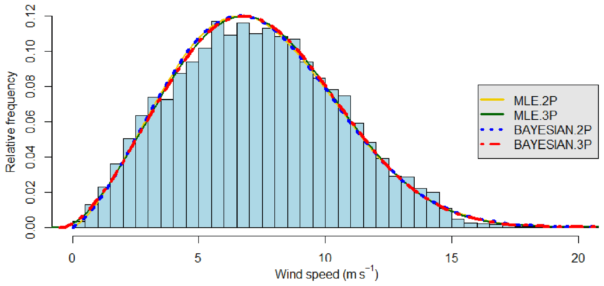
Figure 7The 2-p and 3-p Weibull curves by four methods and histogram of the observed wind speeds at site 5. There are relatively high frequencies of lower and higher wind speeds compared to the mean wind speed. However, the skewness is still relatively low for this site. The percentage of lowest wind speeds of 0–1 m s−1 is 0.79 %, and it can be seen that the Bayesian 3-p Weibull distribution fits the histogram better. The fit is supported by the analysis presented in Tables 5 and 7.
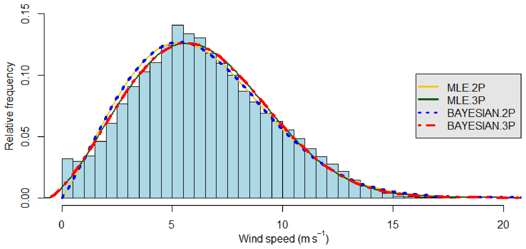
Figure 8The 2-p and 3-p Weibull curves by four methods and histogram of the observed wind speeds at site 7. This site has the second-highest percentage of the lowest wind speeds. It can be seen that the Bayesian 3-p distribution is a better fit here with the 3-p curve touching almost all the bars at the peak. The error analysis of Table 7 clearly shows that the 3-p Bayesian curve is the best fit for this site's wind speed data.
Figures 5 and 7 show symmetric Weibull distribution curves for sites 2 and 5. The mean wind speed is close to the centre, and the percentage of the lowest wind speeds (0–1 m s−1) is relatively small to moderate at these sites, as can be seen in Table 6. The distribution curves clearly indicate that the BAYESIAN.3P Weibull distribution fits the data best, which is also supported by the goodness-of-fit measures presented in Table 7.
However, Figs. 6 and 8 show non-symmetric distributions of wind speeds for sites 3 and 7. The distribution curves clearly indicate that the BAYESIAN.3P Weibull distribution fits better to the data at these sites. It can be noted that these sites recorded a very high percentage of low wind speeds (0–1 m s−1), as seen in Table 6.
On the other hand, it has also been seen that the wind speed distribution for sites 4 and 6 (figures not shown) is less symmetric compared to the other sites, with clearly high skewness as seen in Table 6. For these sites, the percentage of the lowest wind speeds is smaller; hence the Bayesian 2-p distribution fits the wind speed data well. Although the four Weibull distribution curves seem to coincide, the BAYESIAN.2P distribution curves lie above the 3-p one before the peak and below the 3-p curve after the peak. From Table 4, it can be seen that the values of the shift parameters θ are the smallest (close to zero) for these sites; hence the 3-p Weibull distribution becomes the 2-p distribution. The 3-p Weibull distribution is thus a possible replacement for the existing models that find Weibull parameters, especially those used in commercially used software like WAsP.
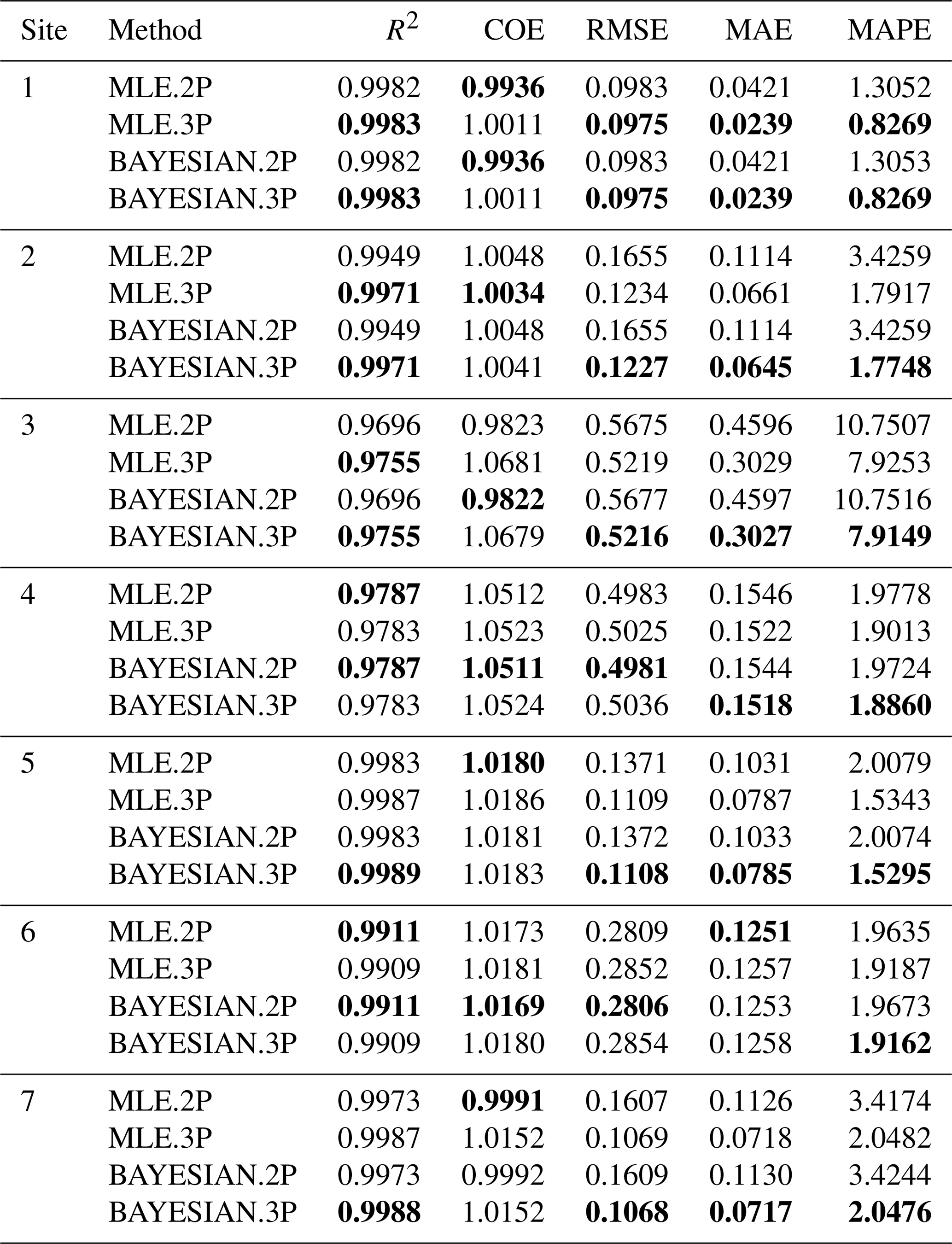
To evaluate the performance of the four methods, the five statistical goodness-of-fit measures discussed in Sect. 6 (R2, RMSE, COE, MAE and MAPE) are estimated and compared. The results of the estimation of these measures for the wind data from all the seven sites are presented in Table 7, which clearly reveal that BAYESIAN.3P is the most efficient method for sites 2, 3, 5 and 7 as it gives the highest R2 value and the lowest RMSE, MAE and MAPE values. This indicates that the 3-p Weibull distribution with Bayesian estimates is a better method for wind energy assessment at these sites. Moreover, the method performs equally to MLE.3p for site 1, whereas BAYESIAN.2P performs better for sites 4 and 6, producing the highest R2 value and the lowest COE and RMSE values, which indicates the 2-p Weibull distribution with Bayesian estimates is a better method for assessment at these two sites that have the lowest occurrence of the lowest wind speeds in the range of 0–1 m s−1.
Table 7Estimated values of goodness-of-fit measures R2, RMSE, COE, MAE and MAPE evaluated for the performance of the four methods.
Assessment of wind power density
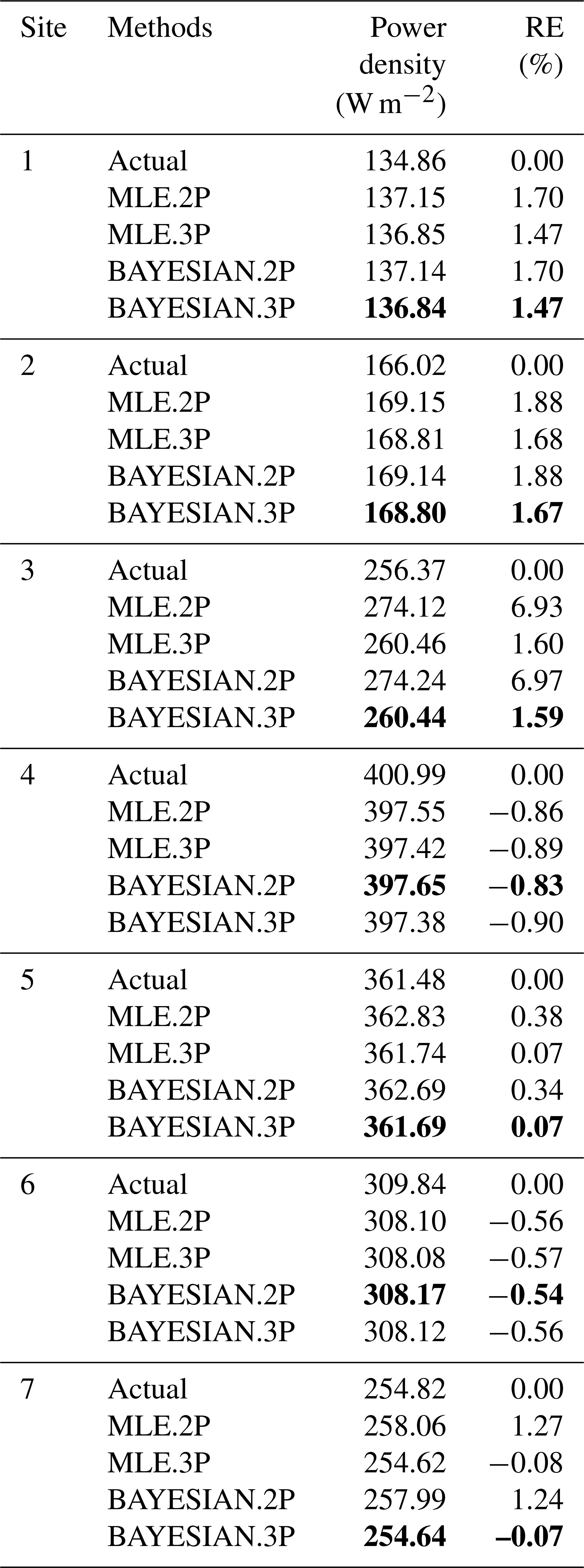
To estimate the turbine productivity, it is necessary to calculate the wind power density from each fitted model. If the density of the air ρ=1.16 kg m−3 (based on the average temperature in the region), the expected wind power density produced from each site is determined using Eqs. (24)–(25) for both 2-p and 3-p Weibull distributions. Table 8 shows estimated results for wind power density.
The relative error of the estimated power density, shown in Table 8, is calculated as follows:
If RE is close to zero, the method estimates the parameter accurately. However, a positive RE implies over-estimation and a negative RE implies under-estimation by this method. From the values of power and RE presented in Table 8, we found that BAYESIAN.2P and BAYESIAN.3P are the most efficient methods for estimating power. The BAYESIAN.3P predicts the most accurate wind power for sites 1, 2, 3, 5 and 7, which is very close to the actual power of these sites, with smaller RE compared to the other methods. On the other hand, BAYESIAN.2P provides the best estimate of power for sites 4 and 6 with smaller relative error.
Table 8The actual wind power and estimated wind power density determined for the four methods listed for each site with the relative error in power estimation.
Thus, the comparison of results based on the goodness of fit and the power estimation at different sites in the tropical region show that the 3-p Weibull distribution with Bayesian estimates is the method to be used for wind energy resource assessments. If any site has lower occurrence of the lower wind speeds, then the shift parameter θ in the 3-p Weibull distribution will be close to or equal to zero, which constitutes the 2-p Weibull distribution with Bayesian estimates. Another advantage of the Bayesian approach is that it will reduce the need for long-term measurements for assessing the wind power potential of a site. This is possible with the integration of prior information with short-term data from a candidate site or with historical data from one neighbouring survey station.
Knowledge of the correct statistical distribution of wind speeds at a given site is very important for accurate wind resource assessment. Some sites provide high uncertainty while fitting the traditional two-parameter Weibull distributions to wind speed data and warrant the need to explore distributions that characterize wind speeds better, such as the three-parameter Weibull distribution, which is also a generalized form of the two-parameter Weibull distribution with an additional non-zero shift parameter. In this study, investigations of wind characteristics and wind energy potential are carried out at different locations in the tropical region ranging from 1∘ N to 21∘ S of the Equator, of which three sites are in Fiji and the others are in the Cooks Islands, Tonga, Kiribati and Vanuatu (one site in each). The wind speed data at these seven sites were tested for the best model between the two-parameter and three-parameter Weibull distributions. Furthermore, as there is no unique method that characterizes wind data perfectly, it is also imperative to have knowledge of the best method of estimation for the parameters of wind speed distribution at a given site. In this work, we also introduced a novel approach by using the Bayesian method for estimating parameters of wind speed distributions at the seven sites selected for testing the method. Then, a comparison study was conducted for the robust performance of the proposed Bayesian method with the popular frequentist MLE method. Finally, the results suggest that the three-parameter Weibull distributions should be used for estimating the wind energy potential irrespective of the location. When the wind distribution has frequent low wind speeds and is less skewed, a three-parameter Weibull distribution is found to be a better fit. On the other hand, when the wind speed distribution has less frequent low speeds and is highly skewed, the two-parameter Weibull distribution which is a special case of three-parameter distribution with a zero shift parameter is found to be more appropriate. The results also indicate that the Bayesian approach provides more accurate results while characterizing wind speeds and can be proposed as a better alternative for estimating Weibull parameters. The proposed method can be incorporated into popular software packages such as WAsP that are used for wind resource assessment and for planning wind energy projects.
JAGS model specifications to perform the Bayesian fit using R2jags package
are provided below.
A1 Model specification for two-parameter Weibull distribution
cat("
model{
# Likelihood
for (i in 1:length(U)){
p[i] <- dweib(U[i],shape, lambda);
observed[i] ∼ dbern(p[i]);
}
# Priors
shape ∼ dunif(0,4) # After a series of
trial and error guesses
scale ∼ dunif(0,100)
lambda <- pow(1/(scale), shape)
}
", file="weibull_model_2p.txt")
Calling JAGS from R
jags.fit <- jags(data, inits,
parameters.to.save, n.iter=10000,
model.file="weibull_model_2p.txt",
n.chains = 3, n.burnin = 1000,
n.thin=5)
A2 Model specifications for the three-parameter Weibull distribution
cat("
model{
# Likelihood
for (i in 1:length(U)){
p[i] <- dweib(U[i] - shift, shape,
lambda) / 1000
observed[i] ∼ dbern(p[i]);
}
# Priors
shape ∼ dunif(0,4)
scale ∼ dunif(0,31)
shift ∼ dunif(-1, 1)
lambda <- pow(1/(scale), shape)
}
", file="weibull_model_3p.txt")
The model code is provided in Appendix A. The full code can be made available upon a very valid request.
Sample data files are available online at http://repository.usp.ac.fj/id/eprint/14126 (Ahmed, 2016). Full data will be made available upon request and after approval from the respective governments.
MGMK: conceptualization of new method, writing the code, simulations and draft paper; MRA: project approval, data acquisition, compilation, validation and review of manuscript.
The contact author has declared that neither of the authors has any competing interests.
Publisher’s note: Copernicus Publications remains neutral with regard to jurisdictional claims in published maps and institutional affiliations.
Funds for carrying out part of this work were provided by the Korea International Cooperation Agency (KOICA) under its East-Asia Climate Partnership programme. The project number is 2009-00042.
This paper was edited by Andrea Hahmann and reviewed by two anonymous referees.
Ahmed, M. R.: Sample Data for Pentecost, Rakiraki and Rarotonga (Appendix 3), http://repository.usp.ac.fj/id/eprint/14126 (last access: 14 August 2023), 2016.
Aukitino, T., Khan, M. G. M, and Ahmed, M. R.: Wind energy resource assessment for Kiribati with a comparison of different methods of determining Weibull parameters, Energ. Convers. Manage., 151, 641–660, https://doi.org/10.1016/j.enconman.2017.09.027, 2017.
Azad, A. K., Rasul, M. G., and Yusaf, T.: Statistical diagnosis of the Best Weibull methods for wind power assessment for agricultural applications, Energies, 7, 3056–3085, https://doi.org/10.3390/en7053056, 2014.
Carta, J. A., Ramirez, P., and Velazquez, S.: A review of wind speed probability distributions used in wind energy analysis: Case studies in the Canary Islands, Renewable and sustainable energy reviews, 13, 933–955, https://doi.org/10.1016/j.rser.2008.05.005, 2009.
Casella, G. and Berger, R. L.: Statistical inference, 2nd edn., Cengage Learning, ISBN 978-0-534-24312-8, 2020.
Chang, T. P.: Performance comparison of six numerical methods in estimating Weibull parameters for wind energy application, Appl. Energ., 88, 272–282, https://doi.org/10.1016/j.apenergy.2010.06.018, 2011.
Chaurasiya, P. K., Ahmed, S., and Warudkar, V.: Comparative analysis of Weibull parameters for wind data measured from met-mast and remote sensing techniques, Renew. Energ., 115, 1153–1165, https://doi.org/10.1016/j.renene.2017.08.014, 2018.
Corotis, R. B., Sigl, A. B., and Klein, J.: Probability models of wind velocity magnitude and persistence, Sol. Energy, 20, 483–493, https://doi.org/10.1016/0038-092X(78)90065-8, 1978.
Cousineau, D. and Allan, T.: Likelihood and its use in parameter estimation and model comparison, Mesure et évaluation en éducation, 37, 63–98, https://doi.org/10.7202/1036328ar, 2015.
Gosai, A.: Wind Energy potential and electricity generation at Rokavukavu, Rakiraki, MSc thesis, The University of the South Pacific, https://librarycat.usp.ac.fj/client/en_GB/search/asset/5045/0 (last access: 8 July 2022), 2014.
Guure, C. B., Ibrahim, N. A., and Ahmed, A. O. M.: Bayesian estimation of two-parameter weibull distribution using extension of Jeffreys' prior information with three loss functions, Math. Probl. Eng., 2012, 589640, https://doi.org/10.1155/2012/589640, 2012.
Hossain, A. and Zimmer, W.: Comparison of estimation methods for Weibull parameters: complete and censored samples, J. Stat. Comput. Sim., 73, 145–153, https://doi.org/10.1080/00949650215730, 2003.
Ibrahim, N. A. and Mohammed, A.: Bayesian survival estimator for Weibull distribution with censored data, Journal of Applied Sciences, 11, 393–396, https://doi.org/10.3923/jas.2011.393.396, 2011.
IEA: Key world energy statistics, International Energy Agency, Paris, https://www.iea.org/reports/key-world-energy-statistics-2021 (last access: 22 February 2023), 2021.
IEC 61400-1: Wind turbines – Part 12-1: Power performance measurements of electricity producing wind turbines, https://www.iec.ch (last access: 10 April 2022), 2017.
Indhumathy, D., Seshaiah, C., and Sukkiramathi, K.: Estimation of Weibull Parameters for Wind speed calculation at Kanyakumari in India, International Journal of Innovative Research in Science, 3, 8340–8345, 2014.
Jain, P.: Wind Energy Engineering, 2nd edn., McGraw Hill, New York, ISBN 978-0-07-184385-0, 2016.
Kidmo, D. K., Danwe, R., Doka, S. Y., and Djongyang, N.: Statistical analysis of wind speed distribution based on six weibull Methods for wind power evaluation in Garoua, Cameroon, Journal of Renewable Energies, 18, 105–125, https://www.asjp.cerist.dz/en/downArticlepdf/401/18/1/121257 (last access: 17 March 2022), 2015.
Kutty, S. S., Khan, M. G., and Ahmed, M. R.: Estimation of different wind characteristics parameters and accurate wind resource assessment for Kadavu, Fiji, AIMS Energy, 7, 760–791, https://doi.org/10.3934/energy.2019.6.760, 2019.
Lawless, J. F.: Statistical models and methods for lifetime data, 2nd edn., John Wiley & Sons, ISBN 0-471-37215-3, 2003.
Leahy, P. G. and McKeogh, E. J.: Persistence of low wind speed conditions and implications for wind power variability, Wind Energy, 16, 575–586, https://doi.org/10.1002/we.1509, 2013.
Luceño, A.: Maximum likelihood vs. maximum goodness of fit estimation of the three-parameter Weibull distribution, J. Stat. Comput. Sim., 78, 941–949, https://doi.org/10.1080/00949650701467363, 2008.
Lye, L. M., Hapuarachchi, K., and Ryan, S.: Bayes estimation of the extreme-value reliability function, IEEE T. Reliab., 42, 641–644, https://doi.org/10.1109/24.273598, 1993.
Manwell, J. F., McGowan, J. G., and Rogers, A. L.: Wind energy explained: theory, design and application, 2nd edn., John Wiley & Sons, ISBN 978-0-470-01500-1, 2010.
Michalena, E., Kouloumpis, V., and Hills, J. M.: Challenges for Pacific Small Island developing states in achieving their nationally determined contributions (NDC), Energ. Policy, 114, 508–518, https://doi.org/10.1016/j.enpol.2017.12.022, 2018.
Ministry Of Economy: Fiji NDC Implementation Roadmap 2017–2030, https://gggi.org/report/fiji-ndc-implementation-roadmap/ (last access: 15 July 2022), 2017.
Pandey, B. N., Dwividi, N., and Pulastya, B.: Comparison between Bayesian and maximum likelihood estimation of the scale parameter in Weibull distribution with known shape under linex loss function, Journal of Scientific Research, 55, 163–172, 2011.
Patlakas, P., Galanis, G., Diamantis, D., and Kallos, G.: Low wind speed events: persistence and frequency, Wind Energy, 20, 1033–1047, https://doi.org/10.1002/we.2078, 2017.
Plummer, M.: JAGS: A program for analysis of Bayesian graphical models using Gibbs sampling, in: Proceedings of the 3rd International Workshop on Distributed Statistical Computing (DSC 2003), 20–22 March 2003, Vienna, Austria, 2003.
PPA (Pacific Power Association): World Bank Provides Grant for Renewable Energy: http://www.ppa.org.fj/world-bank-provides-grant-for-renewable-energy/ (last access: 12 August 2021), 2015.
Ramachandran, K. M. and Tsokos, C. P.: Mathematical statistics with applications in R, 3rd edn., Academic Press, ISBN 978-0-12-817815-7, 2021.
Renner, M., Garcia-Banos, C., and Khalid, A.: Renewable energy and jobs: annual review 2022, https://www.irena.org/publications/2022/Sep/Renewable-Energy-and-Jobs-Annual-Review-2022 (last access: 25 January 2023), 2022.
Robinson, S. A.: Climate change adaptation in SIDS: A systematic review of the literature pre and post the IPCC Fifth Assessment Report, WIRES Clim. Change, 11, e653, https://doi.org/10.1002/wcc.653, 2020.
Rocha, P. A. C., de Sousa, R. C., de Andrade, C. F., and da Silva, M. E. V.: Comparison of seven numerical methods for determining Weibull parameters for wind energy generation in the northeast region of Brazil, Appl. Energ., 89, 395–400, https://doi.org/10.1016/j.apenergy.2011.08.003, 2012.
Singh, K., Bule, L., Khan, M. G., and Ahmed, M. R.: Wind energy resource assessment for Vanuatu with accurate estimation of Weibull parameters, Energ. Explor. Exploit., 37, 1804–1832, https://doi.org/10.1177/0144598719866897, 2019.
Singh, K. A., Khan, M., and Ahmed, M. R.: Wind Energy Resource Assessment for Cook Islands With Accurate Estimation of Weibull Parameters Using Frequentist and Bayesian Methods, IEEE Access, 10, 25935–25953, 2022.
Spiegelhalter, D. J., Best, N. G., Carlin, B. P., and Van Der Linde, A.: Bayesian measures of model complexity and fit, J. Roy. Stat. Soc. B, 64, 583–639, https://doi.org/10.1111/1467-9868.00353, 2002.
Su, Y. and Yajima, M.: Using R to run “JAGS”, R package version 0.6-1, https://cran.r-project.org/web/packages/R2jags (last access: 22 November 2021), 2020.
Sukkiramathi, K. and Seshaiah, C.: Analysis of wind power potential by the three-parameter Weibull distribution to install a wind turbine, Energ. Explor. Exploit., 38, 158–174, https://doi.org/10.1177/0144598719871628, 2020.
Teimouri, M. and Gupta, A. K.: On the three-parameter Weibull distribution shape parameter estimation, Journal of Data Science, 11, 403–414, https://doi.org/10.6339/JDS.2013.11(3).1110, 2013.
Tuller, S. E. and Brett, A. C.: The characteristics of wind velocity that favor the fitting of a Weibull distribution in wind speed analysis, J. Appl. Meteorol. Clim., 23, 124–134, https://doi.org/10.1175/1520-0450(1984)023<0124:TCOWVT>2.0.CO;2, 1984.
Wais, P.: Two and three-parameter Weibull distribution in available wind power analysis, Renew. Energ., 103, 15–29, https://doi.org/10.1016/j.renene.2016.10.041, 2017.
Wang, W., Chen, K., Bai, Y., Chen, Y., and Wang, J.: New estimation method of wind power density with three-parameter Weibull distribution: A case on Central Inner Mongolia suburbs, Wind Energy, 25, 368–386, https://doi.org/10.1002/we.2677, 2022.
Weir, T.: Renewable energy in the Pacific Islands: Its role and status, Renewable and Sustainable Energy Reviews, 94, 762–771, https://doi.org/10.1016/j.rser.2018.05.069, 2018.
- Abstract
- Introduction
- Wind speed data sites
- Weibull distribution
- Methods of estimating Weibull parameters
- Estimation of wind power density
- Analysing the performance of different estimators
- Results
- Discussion
- Conclusions
- Appendix A: Model code
- Appendix B: Trace and posterior density plots that show the convergence of Bayesian models for sites 1, 5 and 6.
- Code availability
- Data availability
- Author contributions
- Competing interests
- Disclaimer
- Financial support
- Review statement
- References