Difference in load predictions obtained with effective turbulence vs. a dynamic wake meandering modeling approach

According to the international standard for wind turbine design, the effects of wind turbine wakes on structural loads can be considered in two ways: (1) by augmenting the ambient turbulence levels with the effective turbulence model (EFF) and then calculating the resulting loads and (2) by performing dynamic wake meandering (DWM) simulations, which compute wake effects and loads for all turbines on a farm at once. There is no definitive answer in scientific literature as to the consequences of choosing one model over the other, but the two approaches are unarguably very different. The work presented here expounds on these differences and investigates to what extent they affect the simulated structural loads. We consider an idealized 4×4 rectangular array of National Renewable Energy Laboratory 5 MW wind turbines with a spacing of 5 by 8 rotor diameters and three wind speed scenarios at high ambient turbulence. Load simulations are performed in OpenFAST with EFF and in FAST.Farm with the DWM implementation. We compare ambient turbulence, wind farm turbulence, and loads between both approaches. When omnidirectional results are compared, EFF wind farm turbulence intensity is consistently higher by 0.2 % (above-rated wind speed) to 2.7 % (below-rated wind speed). However, for certain wind directions, the EFF turbulence can be lower than FAST.Farm by almost 9 %. Wind speeds within the farm were found to differ by up to 3 m s⁻¹ due to the lack of wake deficits in the EFF approach, leading to longer tails toward low values in the FAST.Farm mean load distributions. Consistent with the turbulence results, the median EFF load standard deviations are also consistently higher, by a maximum of 20 % and 17 % for blade-root out-of-plane and tower-base fore-aft moments, respectively.

1 Introduction

Modeling approaches that have become standard industry practice tend to be relatively simple to implement and inexpensive to run. Over time, as simulation tools improve and computational costs decrease, modeling approaches that are incrementally more complex and expensive become increasingly accessible. When that happens, we have the opportunity to revisit standard procedures and evaluate whether the wind industry as a whole might benefit from updated practices that incorporate higher-fidelity models into the design process.

The International Electrotechnical Commission (IEC) standard (International Electrotechnical Commission, 2019) recommends two methods to capture wake effects in wind turbine design and site suitability analyses: the effective turbulence model (EFF; Frandsen, 2007; Frandsen and Thøgersen, 1999) and the dynamic wake meandering (DWM) model (Larsen et al., 2008). The EFF is a much simpler approach that encapsulates wake effects into increased (i.e., “effective”) turbulence levels relative to the freestream. The DWM model is more complex, requiring wind farm simulations that resolve the wake dynamics of individual turbines with simplified physical and empirical parameterizations. This difference in complexity means that running DWM simulations requires more expertise, time, and computational resources. However, the DWM model can still be run on a single computer node, and the effort levels are fairly low when compared to high-fidelity methods such as large-eddy simulations.

If we agree that the two modeling approaches – EFF and DWM – are computationally tractable, then the next obvious question is whether the added investment of running DWM simulations is worth the effort and cost. The work presented here helps to answer this question. To do so, we quantify the differences between both methods throughout each step in the simulation chain: from inflow generation to load predictions. We use the effective turbulence definition found in the IEC standard (International Electrotechnical Commission, 2019) and the DWM model as implemented in FAST.Farm (Jonkman and Shaler, 2021). In addition to quantifying differences in turbulence levels, load means, and fluctuations, we quantify the computational cost of both methods.

Even if we assume that the higher-fidelity DWM model is more accurate, choosing it over the EFF will depend on the magnitude of their differences and the acceptable margin of error for the application in question. There is no obvious consensus in scientific literature as to the magnitude and sign of EFF errors relative to measurements or higher-fidelity models. The first studies comparing the EFF to other reference data (Thomsen et al., 2007; Sørensen et al., 2008; Schmidt et al., 2011a, b) identified overestimations and underestimations of loads depending on the incoming wind speed, the interturbine spacing, and the turbine component being considered. Later studies seemed to agree on an overestimation of wind farm turbulence levels (Argyle et al., 2018; Reinwardt et al., 2018) and fatigue loads (Reinwardt et al., 2018; Slot et al., 2018, 2019). In terms of load components, errors seem consistently larger for the tower than for the blades (Thomsen et al., 2007; Schmidt et al., 2011b; Reinwardt et al., 2018; Slot et al., 2019). The study of Slot et al. (2019) was the only study to include main shaft torque, and they found those errors to be larger than those of the tower. With regard to fatigue error magnitudes, studies report a large range: ∼3 % (Fig. 3 in Slot et al., 2019) to ∼37 % (Fig. 11 in Reinwardt et al., 2018) for the tower base, with some studies finding values in between (i.e., 20 % in Thomsen et al., 2007, and Schmidt et al., 2011b).

Three existing studies have compared load predictions between the EFF and DWM implementations. Each of these studies used a different aeroelastic simulation tool: HAWC in Thomsen et al. (2007), Bladed in Schmidt et al. (2011a, b), and FLEX5 in Reinwardt et al. (2018). No details are provided in these studies as to the inflow generation methods used. For a fixed turbulence level, Thomsen et al. (2007) found the EFF to overestimate tower and blade loads at higher winds (20 m s⁻¹) and underestimate them at lower winds (10 m s⁻¹). The largest differences were on the order of 27 % for fatigue loads and 65 % for extreme loads. When considering a realistic wind climate and lifetime calculations, Schmidt et al. (2011b) did not find any underestimations on the part of the EFF. Rather, EFF fatigue loads were higher by ∼10 % for the blades and ∼20 % for the tower. Finally, Reinwardt et al. (2018) found overpredictions higher than 35 % for partially waked conditions when considering closely spaced (< 4 rotor diameters) wind turbines.

The work that we present here was motivated by the small number of published studies on this topic and the lack of consistency among them. We compare the EFF to the DWM implementation within FAST.Farm, which was previously validated against large-eddy simulations and measurements (Kretschmer et al., 2021; Shaler and Jonkman, 2021; Shaler et al., 2020). We analyze the results after each step in the simulation chain, which allows us to identify the sources of differences between the two approaches. The simulation and analysis methods are described in Sect. 2. The results are presented in terms of freestream turbulence, wake turbulence, and loads in Sect. 3. A final discussion is given in Sect. 4. We hope that the results we present will allow wind farm modeling experts to be informed and intentional when choosing simulation tools and making design decisions.

2 Methods

This section describes the two simulation approaches used to estimate wind turbine loads (Sect. 2.1), the wind farm layout considered (Sect. 2.2), and the inflow scenarios defined (Sect. 2.3).

2.1 Simulation approaches

The structural loading on each wind turbine is simulated with two different methods: the EFF and a DWM approach as implemented in FAST.Farm (Jonkman and Shaler, 2021). The EFF is the more simplified and inexpensive approach and has, for these reasons, become the industry standard for wind plant fatigue load assessment. As the name implies, the DWM approach simulates the dynamic interactions between inflow, turbines, and wake. Despite its higher complexity and computational cost, it is still inexpensive enough to be appropriate for design calculations. Broadly speaking, the main difference between these methods is how they treat the effects of wind turbine wakes on the structural loads. More specific details on how the two methods differ are discussed next.

2.1.1 Effective turbulence

The EFF implemented here is based on the equations provided in the IEC design standard for wind turbines (International Electrotechnical Commission, 2019). The effective turbulence I_eff,

$$\begin{array}{}\text{(1)}& I_{\mathrm{eff}}={\displaystyle \frac{{\mathit{\sigma }}_{\mathrm{eff}}}{V_{\mathrm{hub}}}},\end{array}$$

is obtained from the hub-height wind speed V_hub and effective standard deviation σ_eff,

$$\begin{array}{}\text{(2)}& {\mathit{\sigma }}_{\mathrm{eff}}={\left[(\mathrm{1}-N\cdot \mathrm{0.06}){\mathit{\sigma }}_{\mathrm{c}}^m+\mathrm{0.06}\sum _{i=\mathrm{1}}^N{\mathit{\sigma }}_T^m\right]}^{m^{-\mathrm{1}}},\end{array}$$

where N is the number of neighboring wind turbines, 0.06 is the probability of wake conditions (Sørensen et al., 2008), σ_c is the characteristic wind speed standard deviation, m is the Wöhler exponent, and σ_T is given by

$$\begin{array}{}\text{(3)}& {\mathit{\sigma }}_T={\left[{\displaystyle \frac{V_{\mathrm{hub}}^{\mathrm{2}}}{\mathrm{1.5}+\frac{\mathrm{0.8}d}{\sqrt{C_{\mathrm{T}}}}}}+{\mathit{\sigma }}_{\mathrm{c}}^{\mathrm{2}}\right]}^{\mathrm{1}/\mathrm{2}},\end{array}$$

where d is the distance between the target turbine (i.e., the one for which σ_eff is being computed) and neighboring turbine i and C_T is the thrust coefficient of neighboring turbines. Here, C_T is the same for the 16 wind turbines for a given wind scenario. In total, three individual wind and thrust values are used based on the scenarios defined in Sect. 2.3.1. For each scenario, we also consider three Wöhler exponents: m=4 for the tower (welded steel), m=6 for the nacelle components (cast steel), and m=10 for the blades (fiber composites). The output of the model is the effective wind speed standard deviation (σ_eff) at each wind turbine, combining the wake effects of its neighbors for all wind directions relative to the wind farm. A uniform wind direction distribution is considered for both simulation approaches. After obtaining the σ_eff values, turbulent inflow and wind turbine simulations are then performed independently for each wind turbine in the wind farm. We use TurbSim (Jonkman, 2009) to generate synthetic turbulent inflow based on a Kaimal spectrum with exponential coherence and OpenFAST (NREL, 2023) to simulate the wind turbine dynamic response, including aero-servo-elastics.

2.1.2 FAST.Farm

FAST.Farm is a wind farm simulation tool that expands on DWM principles to model wind turbine performance and structural loading within wind farms. Within FAST.Farm, the entire farm is simulated at once with one OpenFAST instance for each wind turbine. Each OpenFAST instance in the FAST.Farm simulations is set up identically to the OpenFAST simulations performed in the EFF approach. In addition to these OpenFAST instances, FAST.Farm computes wake deficit evolution, advection, deflection, meandering, and merging. A snapshot of flow fields simulated with FAST.Farm for the work performed here is shown in Fig. 1. More information on its capabilities and models can be found in Jonkman and Shaler (2021). Note that wake-added turbulence (the additional small-scale turbulence generated from the turbulent mixing in the wake) is a forthcoming capability of FAST.Farm that was not available in the model version used here. That said, the ambient turbulence intensities simulated in the wind scenarios are high enough that the absence of wake-added turbulence would not likely impact the conclusions of this study (Shaler and Jonkman, 2021).

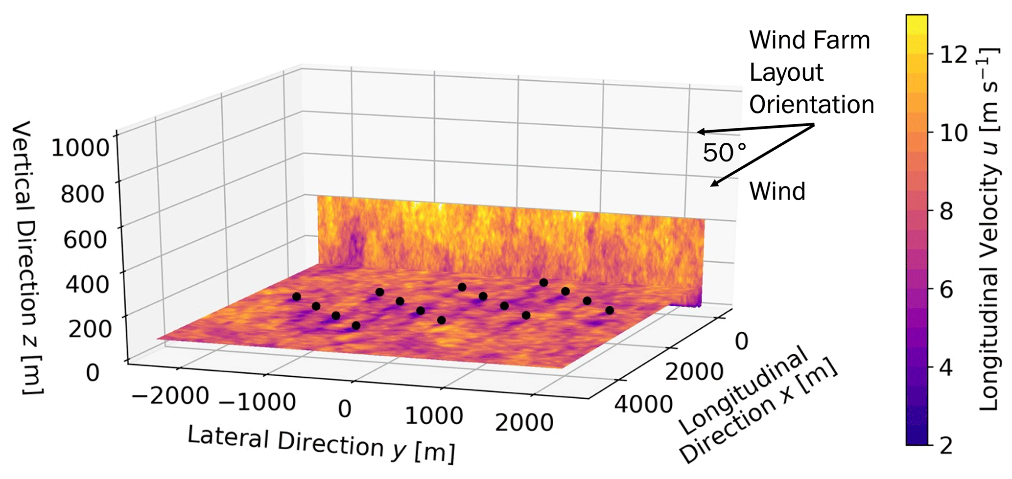
Figure 1 Snapshot (300 s into a 600 s simulation) of flow fields simulated by FAST.Farm for the below-rated wind speed scenario at a 50^∘ orientation between the farm layout and the incoming wind. Black dots mark the turbine locations.

In FAST.Farm, we explicitly consider the effects of varying wind direction on wake dynamics and loads. This is done by performing separate FAST.Farm simulations for every possible incoming flow orientation relative to the wind farm layout. To avoid simulating separate inflows for each of these orientations, we choose to keep the same inflow direction (toward +x) and rotate the wind farm within it. We consider 19 wind farm rotation angles: every 5^∘ from 0 to 90^∘. The results from these simulations are then broadcast to a full wind rose by leveraging the symmetry of the rectangular wind farm layout. More details on this broadcasting process are provided in Sect. 2.2. Specific details of the simulation setup are given in Appendix A.

2.1.3 Differences between approaches

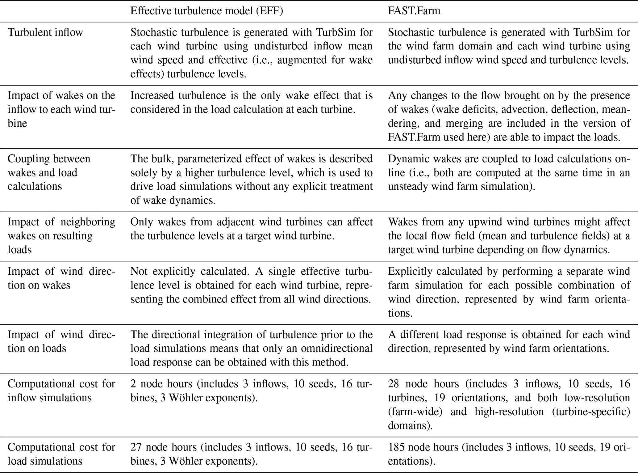
For both methods, the undisturbed inflow and turbine models are identical. The only difference between them is how the inflow to specific wind turbines is calculated. This difference affects several aspects of the simulation, as summarized in Table 1. The differences in computational cost are also given in Table 1, with FAST.Farm requiring $\sim \mathrm{14}\times$ more time for inflow generation (primarily due to the farm-wide inflow simulations) and $\sim \mathrm{7}\times$ more time for load simulations.

Table 1 Differences between the two modeling approaches considered.

2.2 Wind farm layout

We consider an idealized 4×4 rectangular wind farm composed of 16 National Renewable Energy Laboratory 5 MW wind turbines (hub height z_hub= 90 m and rotor diameter D= 126 m) with fixed land-based foundations in flat terrain. The interturbine spacing is 8 D along x and 5 D along y (Fig. 2a). As mentioned in Sect. 2.1.2, wind direction effects are added to the FAST.Farm results by performing 19 sets of simulations where the wind farm orientation with respect to the incoming wind changes in increments of 5^∘. The wind turbine rotors always remain aligned with respect to the incoming mean flow direction. Four examples (for wind farm rotation angles of 0, 25, 50, and 90^∘) are shown in Fig. 2.

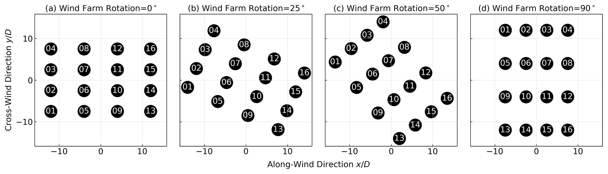
Figure 2 (a) Wind farm layout and (b–d) three example rotation angles out of the 19 simulated in FAST.Farm to account for wind direction effects on the results. Regardless of wind farm rotation, the incoming flow is always from −x to +x. The wind turbine markers are not scaled with the rotor diameter. The wind turbine numbering shown is valid for the 19 simulation setups.

In order to account for wind direction effects across the entire 360^∘ circle, the results from these 19 simulations are broadcast from one to four quadrants. This is made possible by the rectangular layout of the wind farm. For example, a wind farm orientation of 0^∘ is equivalent to one of 180^∘. Likewise, an orientation of 15^∘ is equivalent to −15^∘ (345^∘), 180+15^∘ (195^∘), and 180^∘ − 15^∘ (165^∘). The 0 and 90^∘ simulation results get duplicated (to 180 and 270^∘), while those between 5 and 85^∘ get quadruplicated, leading to a total of 72 simulation results out of the 19 originals. When broadcasting the 0–90^∘ quadrant to the three other quadrants, the wind turbine numbering also needs to be appropriately reconsidered. For example, Turbine 1 (T1) in the original layout (Fig. 2a) does not get waked for any of the 19 simulations performed. However, that same wind turbine will be waked if the wind direction remains constant (toward +x) and the wind farm is rotated past 90^∘. To appropriately account for that, the wind farm numbering is mirrored across the x axis, y axis, or both, depending on the quadrant being considered. Figure 3 specifies the mapping of wind turbine numbering from the original layout (Fig. 2a) in quadrant 1 (0–90^∘) to farm rotations in the other three quadrants.

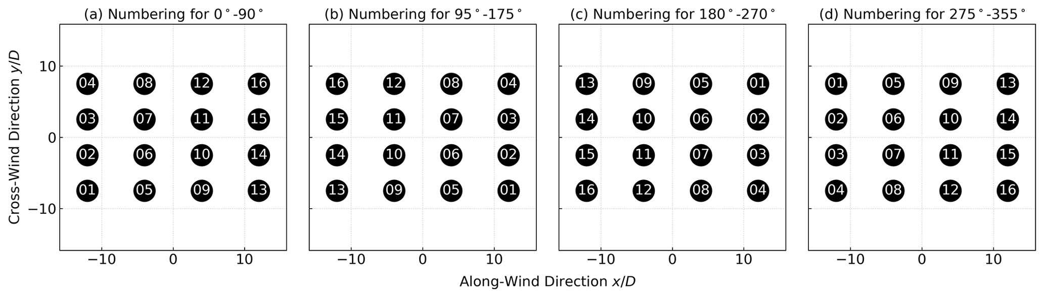
Figure 3 Wind turbine mapping used to broadcast the 19 simulation results spanning 0–90^∘ to the other three quadrants.

2.3 Inflow

2.3.1 Inflow scenarios

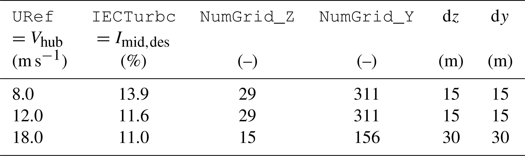
We consider three different inflow scenarios: below (V_hub=8 m s⁻¹, I_hub=15.4 %, C_T=0.79), near (V_hub=12 m s⁻¹, I_hub=13.1 %, C_T=0.54), and above (V_hub=18 m s⁻¹, I_hub=12.5 %, C_T=0.14) rated, where V_hub and I_hub are undisturbed (i.e., freestream) wind speed and turbulence intensity, respectively, at the wind turbine hub height. These turbulence values refer to the “characteristic” turbulence definition as per the international standard (International Electrotechnical Commission, 2019). The wind direction is assumed to be uniformly distributed. The vertical shear follows a power law with an exponent of 0.2. This section describes how the I_hub values used in each scenario were determined to ensure maximum consistency between the two simulation approaches. All values relevant to the inflow turbulence calculation are provided in Table 2. The significance of each value will become clear throughout this section as the inflow generation methods are discussed and contrasted.

Table 2 Starting, intermediate, and final values of the turbulence calculation used when defining the three inflow scenarios considered in this study. Symbols in the table represent inflow wind speed at hub height (V_hub) and at the vertical center of the TurbSim grid (V_mid), maximum acceptable effective standard deviation (σ_eff,max), maximum acceptable characteristic standard deviation (σ_c,max), desired characteristic standard deviation (σ_c,des), obtained characteristic standard deviation (σ_c,obt), desired turbulence intensity at hub height (I_hub,des) and at the vertical center of the TurbSim grid (I_mid,des), and obtained turbulence intensity at hub height (I_hub,obt) and at the vertical center of the TurbSim grid (I_mid,obt).

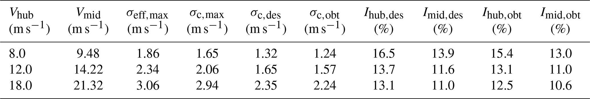
The I_hub values that correspond to each inflow scenario were constrained in two ways. First, they were chosen so that any augmented turbulence levels (found deep in the farm) would still remain within the wind turbine design envelope while assuming a normal turbulence model and a Class A site (International Electrotechnical Commission, 2019). Second, the desired values could not be obtained exactly due to simulation tool (TurbSim) constraints. Next, we explain all steps that were taken to determine the desired turbulence levels (σ_c,des, I_hub,des, I_mid,des) given in Table 2.

1. Define maximum bound on the effective standard deviation (σ_eff,max): for each V_hub value selected, the design turbulence standard deviation σ₁(V_hub) is computed for turbulence Class A as ${\mathit{\sigma }}_{\mathrm{1}}=\mathrm{0.16}(\mathrm{0.75}{V}_{\mathrm{hub}}+\mathrm{5.6}\mathrm{m}{\mathrm{s}}^{-\mathrm{1}})$ and taken as σ_eff,max.

2. Define maximum bound on the characteristic standard deviation (σ_c,max): a range of representative ambient turbulence standard deviation σ_c<σ₁ is used to compute σ_eff for a wind turbine in the center of the defined farm, where the EFF model will yield the highest effective turbulence. The σ_c value that yields ${\mathit{\sigma }}_{\mathrm{eff}}={\mathit{\sigma }}_{\mathrm{eff},\max }$ is taken as σ_c,max, as shown in Fig. 4.

3. Define desired characteristic standard deviation (σ_c,des): to be conservative, instead of using σ_c,max to drive the simulations, we choose to use 80 % of this value. This choice maintains a high turbulence level that is relevant for fatigue loading while still staying below the design constraints. Therefore, ${\mathit{\sigma }}_{\mathrm{c},\mathrm{des}}=\mathrm{0.8}{\mathit{\sigma }}_{\mathrm{c},\max }$. We choose a high turbulence level to assess the difference between the two simulation methods when they are expected to differ the most in terms of fatigue estimates.

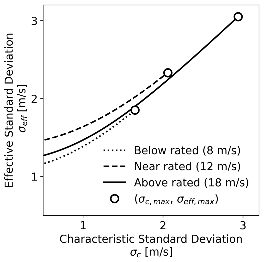
Figure 4 Sensitivity of effective standard deviation (σ_eff) to characteristic ambient standard deviation (σ_c) for each wind speed being considered and a Wöhler exponent of m=10. The circles mark the maximum acceptable characteristic value σ_c,eff to keep the effective value σ_eff,max within the design bounds.

2.3.2 Turbulent inflow simulations

Once the desired turbulence levels are known, the first inflow generation steps can be taken. A summary of all simulation steps, showing the order in which they are conducted, is given schematically in Fig. 5. In FAST.Farm, the turbulent inflow (ambient wind) is generated once for the entire farm so that all wind turbines can be simulated at the same time. TurbSim is run separately for the farm-wide and wind-turbine-specific domains, but FAST.Farm uses all inflows together during the computations. The farm-wide inflow runs are performed first and subsequently used to drive the turbine-specific inflow runs to ensure they are consistent (the turbine-specific inflows are driven by the farm-wide inflows via the constrained turbulence functionality of TurbSim). Given this procedure, the first step in inflow generation (Step FF.1 in Fig. 5) is to use the computed σ_c,des values to drive the farm-wide TurbSim simulations for FAST.Farm. The farm domain was run 30 times: 10 random seeds for 3 different inflow scenarios. Ten seeds were used to obtain more statistical convergence than would be obtained by the IEC recommendation of six seeds. More details on the TurbSim setup for these simulations are given in Appendix B.

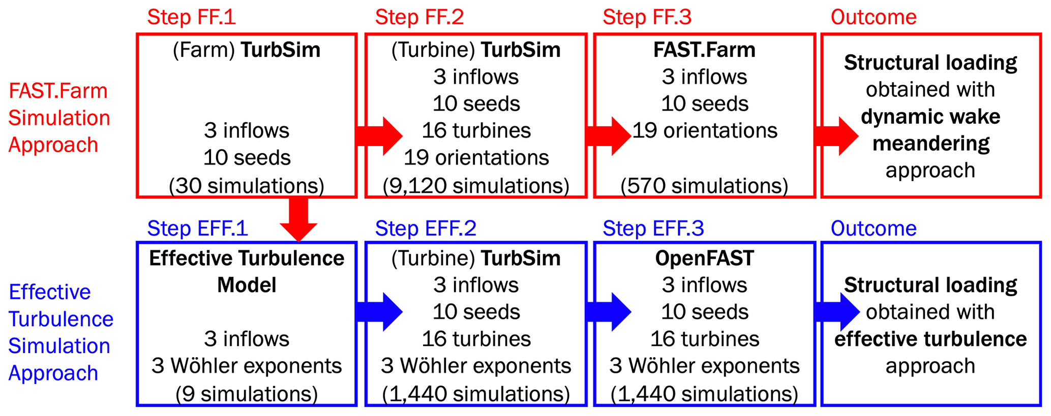
Figure 5 Schematic of methodology used to estimate structural loading on each wind turbine with the two different modeling methods.

The turbulence levels obtained from TurbSim in Step FF.1 are then quantified and used to drive the effective turbulence model (Step EFF.1 in Fig. 5). These obtained σ_c,obt values (i.e., produced by TurbSim) might differ from the desired σ_c,des values (i.e., requested from TurbSim) for two reasons. First, the TurbSim code cannot enforce a specific turbulence level at any height that is lower than half of the grid height. Therefore, we cannot enforce a specific value at the hub height of 90 m given that our grid height is set to 420 m; thus, the reference height at which turbulence levels are requested is the vertical center of the grid, z_mid=210 m. The farm-wide domain must be wide and tall to accommodate any lateral and vertical wake deflection and meandering in addition to the farm rotations performed to account for wind direction effects. Second, the turbulence levels produced by TurbSim might differ by a few percent depending on the random seed from the synthetic generation approach that is based on a finite number of frequency components. An example of this mismatch is shown in Fig. 6 where the requested value σ_c,des is shown along with the lateral distribution and lateral average of σ_u.

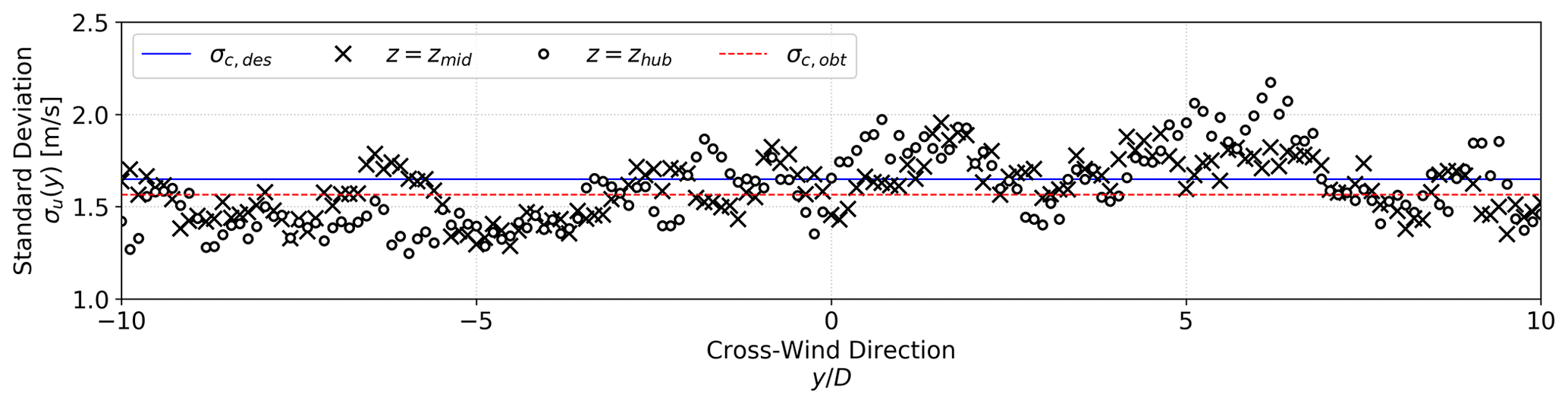
Figure 6 Standard deviation of longitudinal wind velocity for farm-domain TurbSim simulation for one of the random seeds and the near-rated inflow scenario. Values are given at the vertical center of the TurbSim grid (z_mid=210 m) and at the wind turbine hub height (z_hub=90 m) as a function of the cross-wind direction (which is limited to ±10 D for clarity). The dashed horizontal lines mark the desired (σ_c,des) and obtained (σ_c,obt) characteristic standard deviation (averaged along the cross-wind direction) for this specific inflow scenario and seed.

Instead of picking a specific lateral location in the farm-wide domain to evaluate the obtained standard deviation σ_c,obt, we average all values laterally at hub height. This process yields 10 standard deviation values (one per turbulent seed) per inflow scenario, which are given in Fig. 7 at z_mid and z_hub. The seed-averaged standard deviation (marked by the horizontal dashed line in Fig. 7 and given numerically in Table 2) is then taken as the σ_c,obt that is used to drive the effective turbulence model in Step EFF.1. Results from this first effective turbulence simulation step are shown in Fig. 8. By obtaining σ_c,obt from the TurbSim simulations, we ensure that, to the extent possible, FAST.Farm and the EFF are driven with the same inflow wind speed and turbulence levels.

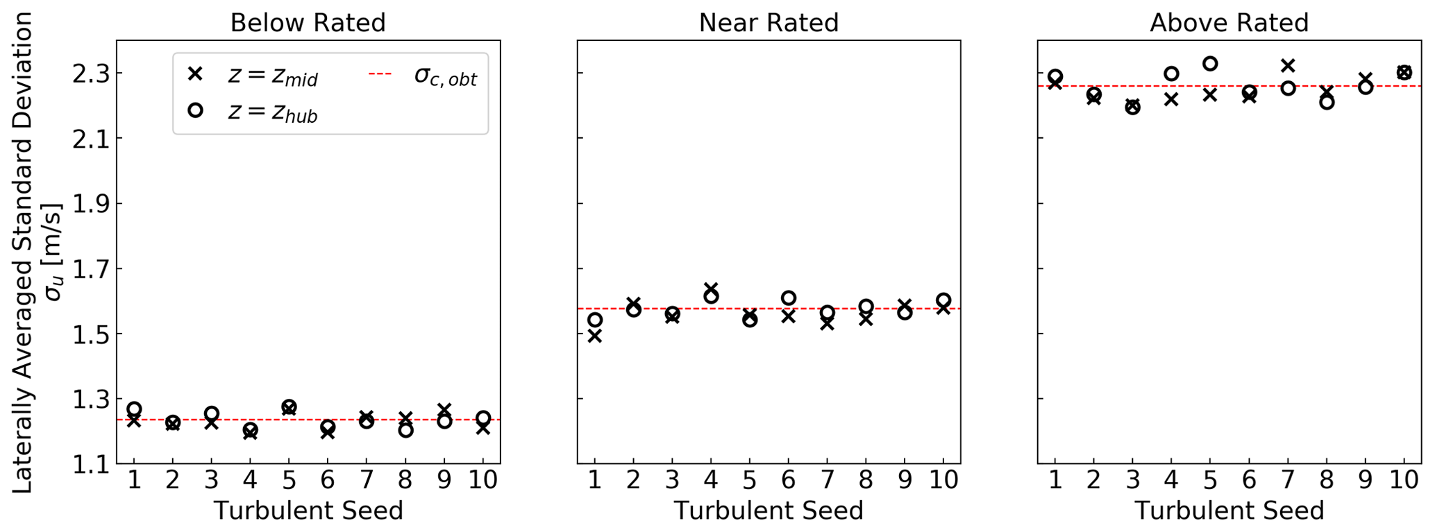
Figure 7 Standard deviation of longitudinal wind velocity for farm-wide domain TurbSim simulations averaged laterally and given at the vertical center of the TurbSim grid (z_mid=210 m) and at the wind turbine hub height (z_hub=90 m) for each of the 10 random seeds. The horizontal lines give the averaged value across all seeds (σ_c,obt).

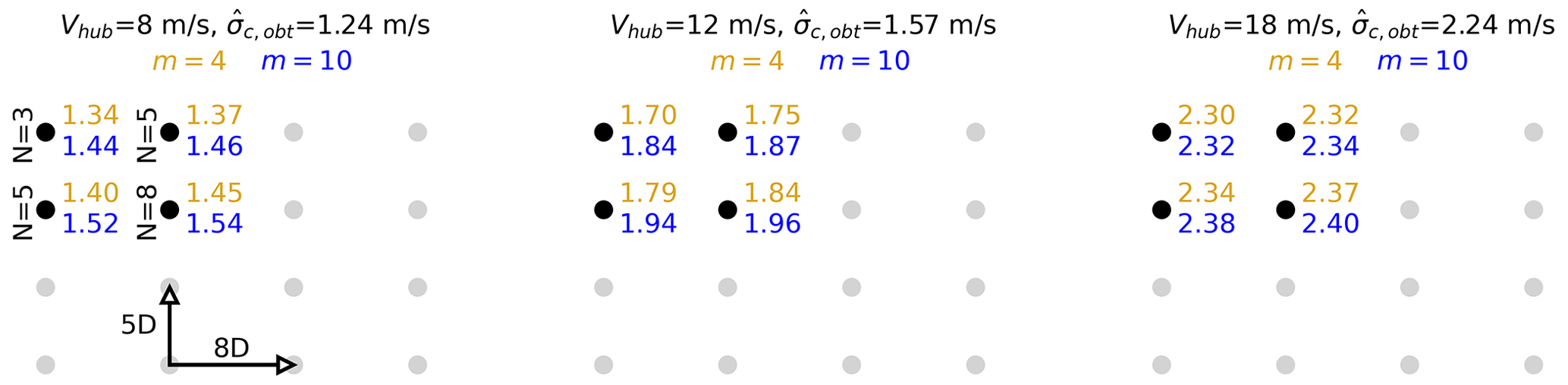
Figure 8 Effective turbulence model (EFF) results in terms of effective standard deviation for the three inflow scenarios when using the lowest (m=4, yellow) and highest (m=10, blue) Wöhler exponents considered. For clarity, results are only shown for a corner of the wind farm. The other corners are symmetrically identical. Arrows show spacing along x (8 D) and y (5 D). The N value provided refers to the number of neighboring wind turbines, which is used in the calculations.

The flow fields generated with Step FF.1 (farm-domain TurbSim runs) are also used to drive Step FF.2 (turbine-specific TurbSim runs). This step needs to include all 16 wind turbines in the farm and all 72 park orientations, which are proxies for varying wind directions. The wind direction did not need to be considered for the farm-wide domain TurbSim inflow files because the domain is large enough to accommodate any park rotation. However, the turbine-specific TurbSim domains are small and therefore need to be generated separately for each rotation angle because of the changing wind turbine locations within the farm-wide domain. A total of 9120 high-resolution TurbSim simulations are performed in Step FF.2: one for each wind turbine (16), inflow scenario and seed (3⋅10), and park orientation (19). To ensure consistency between the farm-wide inflow and the turbine-specific inflows, we use the constrained turbulence functionality (time series input option) of TurbSim when generating the turbine-specific inflow files. In practical terms, this means that for each inflow, seed, and park configuration, the low-resolution TurbSim data are sampled at the point closest to the turbine hub. Vertically, that ends up being exactly at hub height (90 m) for all cases because all farm-wide domain TurbSim grids have a point at the turbine hub height. Laterally, that might end up being a few meters off the turbine hub location to either side due to the relatively coarse resolution of the farm-wide domain TurbSim grid. The axial location of the wind turbine (x_WT) is converted to a position in the time domain $t_{\mathrm{WT}}=x_{\mathrm{WT}}/V_{\mathrm{mid}}$, where V_mid is the advection speed of the flow field within FAST.Farm.

Finally, TurbSim is also run for the effective turbulence approach (Step EFF.2 in Fig. 5). In total, 1440 TurbSim runs were performed to drive the effective turbulence load simulations: one for each wind turbine (16), inflow scenario and seed (3⋅10), and Wöhler exponent (3). The grid size and resolution, time step, and duration are identical to the turbine-specific domain simulations that were run to generate inflow for FAST.Farm. Other run-time options follow the design standard recommendations for the turbulence model and coherence parameters. The turbulence levels requested from each simulation (via the TurbSim parameter IECTurbc) are determined from the EFF results by normalizing the effective standard deviation (for a given wind turbine, inflow scenario, and Wöhler exponent) by the freestream wind speed, ${\mathit{\sigma }}_{\mathrm{eff}}/V_{\mathrm{hub}}$. For example, the top left wind turbine (T4 in Fig. 2) in the below-rated scenario is driven to $\mathtt{\text{IECTurbc}}=\mathrm{1.34}/\mathrm{8}=\mathrm{16.7}\mathit{\%}$ for m=4 and to $\mathtt{\text{IECTurbc}}=\mathrm{1.44}/\mathrm{8}=\mathrm{18.0}\mathit{\%}$ for m=10 (refer back to Fig. 8 to understand these numbers). Note that, here, the run-time option ScaleIEC = 1 was activated, which means that the obtained turbulence level at the hub exactly matches the requested turbulence level. The same was not possible when generating turbine-specific inflow for FAST.Farm, where the only constraint was a matching time series between the farm-domain and turbine-domain runs.

3 Results

3.1 Turbulence levels

To facilitate the interpretation of the fatigue load results, it is first important to understand the differences in turbulence levels between the two simulation methods. Here, we describe the source of these differences and quantify them in terms of the undisturbed (i.e., before consideration of wake effects) and disturbed (i.e., with wakes) inflow.

3.1.1 Turbulence before wakes

In the effective turbulence approach, the freestream turbulence at the hub of each turbine is characterized by a single σ_c,obt value per inflow scenario. In Fig. 9, this value is normalized by V_hub and given in terms of turbulence intensity. Conversely, the freestream turbulence experienced at the hub by each turbine in the FAST.Farm approach varies substantially across space and from simulation to simulation. First, recall that the freestream σ_c,obt from the farm-domain simulations is not a single value per inflow scenario as it is in the effective turbulence approach. Rather, it is a function of the random seed and spatial location (as exemplified in Figs. 6 and 7). These various values might still change slightly when the turbine-specific domain TurbSim simulations are performed. These changes happen only for wind turbine locations that do not coincide exactly with an existing point in the coarser, farm-wide domain grid, thereby requiring TurbSim to generate new turbulence at the requested points. The distributions of these freestream turbulence hub-height values are shown in Fig. 9 for the three inflow scenarios. The distribution means and interquartile range are also shown. Note that the turbulence variability assessment presented here refers only to the hub point. Both modeling approaches still exhibit turbulence variability across the rotor area.

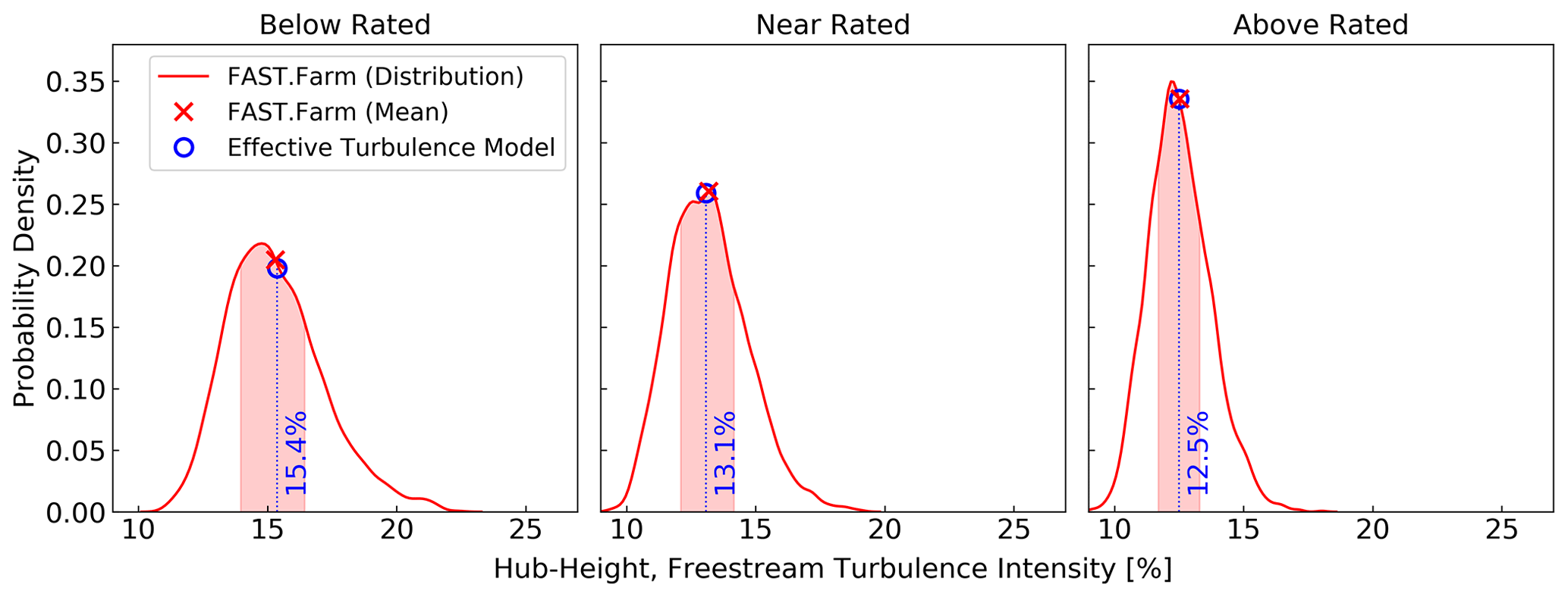
Figure 9 Probability density of hub-height freestream turbulence intensity values at each wind turbine in the FAST.Farm approach (red line). Each distribution includes 11 520 data points: 10 random seeds, 72 wind farm orientations, and 16 wind turbines. The shaded red area under the curve marks the 25th to 75th percentiles of the distribution. The red x marks the mean. The hub-height freestream turbulence intensity in the effective turbulence model (EFF) is the same for all seeds and wind turbines, as shown by the blue circle and given in text.

The values plotted in Fig. 9 highlight the variability in the freestream turbulence driving FAST.Farm, which is not present in the EFF. The probability density curves include spatial variability (across the 16 wind turbines), wind direction variability (across the 72 wind farm/wind direction orientations), and simple turbulence variability (across the 10 random seeds). Variability aside, the mean values from FAST.Farm and the constant value in the EFF match very well for the three inflow scenarios, confirming that the methodology used to generate freestream turbulence was successful in ensuring consistency to the extent possible between the two approaches.

3.1.2 Turbulence with wakes

As previously discussed (Table 1), wake effects on turbulence are considered differently in the two simulation strategies. In FAST.Farm, they are computed within the wind farm simulation because the freestream inflow drives the wind turbines to operate (Fig. 5, Step FF.3). In the effective turbulence approach, wake effects are accounted for via the EFF (Fig. 5, Step EFF.1). The effective standard deviation results obtained were already shown in Fig. 8 for the lowest and highest Wöhler exponents considered. These σ_eff values were then used to produce the stochastic turbulence flow fields (Fig. 5, Step EFF.2), which drove the wind turbine simulations (Fig. 5, Step EFF.3). The comparison presented here considers the turbulence levels at the outcome (Fig. 5) of the two modeling approaches. More specifically, the turbulence intensity shown is computed as the coefficient of variation for the time series of hub-height longitudinal velocity at each wind turbine as output by OpenFAST (in the effective turbulence approach) and FAST.Farm. The results are shown in Fig. 10.

The directional variability in the FAST.Farm results is clear and consistent with expectations. Front-row wind turbines see turbulence levels close to the average freestream turbulence intensity (given by I_hub,obt in Table 2 and shown as a dashed black line in Fig. 10). Second- to fourth-row turbines see turbulence levels higher than freestream due to the presence of wakes. Turbulence is highest for waked turbines when the flow is aligned with a row in the farm. This effect is most pronounced for the below- and near-rated scenarios (Fig. 10a and b), which have stronger wake effects (higher C_T). For the above-rated scenario (Fig. 10c), the directionally averaged turbulence intensity in FAST.Farm is very close to the freestream value for all turbines in the farm.

The comparison between FAST.Farm and the EFF is consistent across wind speed scenarios, with the EFF turbulence levels being a bit higher than the directionally averaged FAST.Farm levels. The differences in turbulence levels are largest for the innermost turbines, where wake effects are larger. For example, T4 has three neighbor turbines and has the closest match between both models. In contrast, T7 has eight neighbor turbines and has the farthest match. Another noteworthy remark is that, while the FAST.Farm directional average is consistently lower than the EFF predictions, the directional results from FAST.Farm are often higher than the highest effective turbulence levels by several percent. This is especially true at below- and near-rated wind speed for wind turbines in the wake when flow is aligned with a row in the farm. As expected, the results are also sensitive to the interturbine spacing. FAST.Farm clearly shows higher wake turbulence along vertical columns of wind turbines (where spacing is tighter at 5 D) than along horizontal rows (where spacing is 8 D).

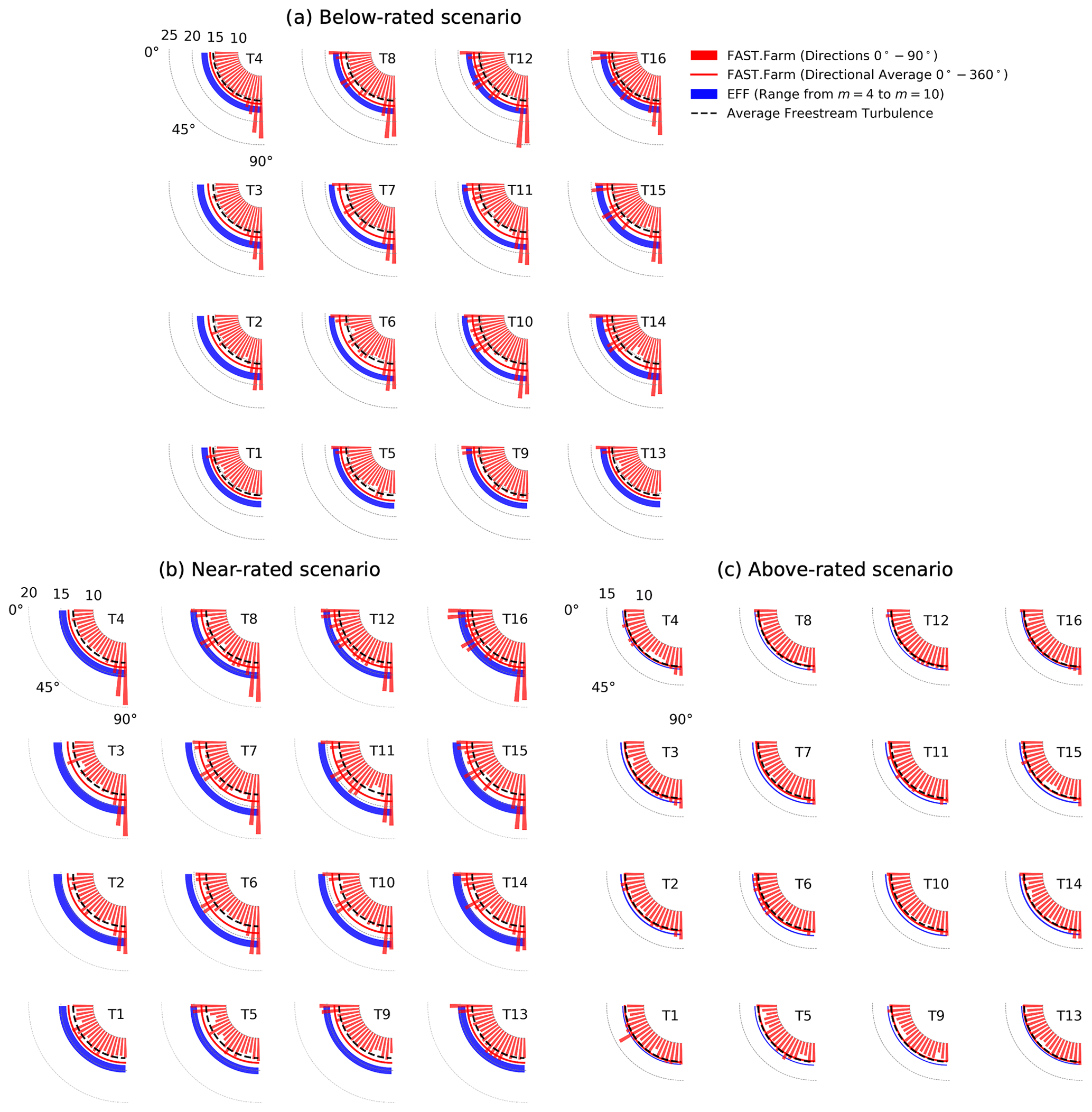
Figure 10 Hub-height turbulence intensity (%) at each wind turbine in the farm for each wind speed scenario. The FAST.Farm bars represent seed-averaged results for wind directions 0–90^∘, while the solid line is the directional average for wind directions 0–360^∘. The effective turbulence model (EFF) shaded region marks the range of results for the lowest (m=4) and highest (m=10) Wöhler exponent (the m=6 values are in between). For reference, the average freestream turbulence (I_hub,obt) is also shown (dashed black line).

We can obtain further insight into these results by considering the entire directional distribution of turbulence across the four quadrants (Fig. 11). This analysis reveals that while the effective turbulence is consistently higher than the FAST.Farm median values, it is always within the FAST.Farm distribution. Note that the FAST.Farm wake turbulence values go below the average freestream turbulence (the dashed black line in Fig. 11) for all wind turbines in the three scenarios. This happens because of lateral and vertical inhomogeneity in the undisturbed inflow. Recall that I_hub,obt is simply a lateral average at hub height through the farm-domain inflow fields. The actual value at a wind turbine location for a particular turbulent seed might be substantially lower as confirmed by the freestream turbulence distributions shown in Fig. 9. As a consequence, the differences seen between FAST.Farm and the EFF are due not only to wake effects but also to the level of fidelity in the turbulent inflow that drives the simulations: a single, precise number for the EFF and a dynamic, heterogeneous flow field for FAST.Farm. Finally, it is worth noting that the EFF only has four unique results for a set of 16 turbines (as was shown in Fig. 8); the other 12 turbines are mirrored due to the wind farm rectangular symmetry. This symmetry is broken in FAST.Farm by the lateral variations in turbulence along rows and columns, leading to eight unique results, as indicated in Fig. 11.

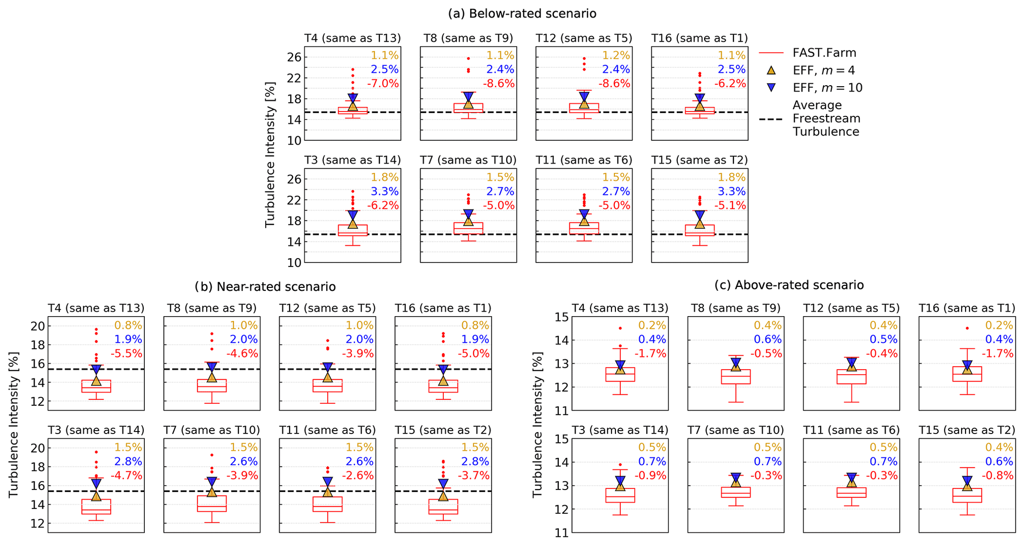
Figure 11 Hub-height turbulence intensity (%) at each wind turbine in the farm for each wind speed scenario. The FAST.Farm results are given in terms of boxplots (the box spans the inter-quartile range with an inner marking for the median) and outliers, with 72 seed-averaged values (one for each wind direction) included in each distribution. The effective turbulence model (EFF) results are given for the lowest (m=4; yellow) and highest (m=10; blue) Wöhler exponent (the m=6 values are in between). For reference, the average freestream turbulence (I_hub,obt) is also shown (dashed black line). For brevity, only the top half of the wind farm is shown. Results are symmetric for the bottom half. The percent values given alongside each distribution quantify the difference between the EFF results and FAST.Farm statistics: the gold percent compares EFF m=4 to the FAST.Farm median; blue compares EFF m=10 to the FAST.Farm median; red compares EFF m=4 to the FAST.Farm maximum.

As previously noted (Table 1), the EFF load calculation is based on undisturbed wind speed values, which are 8, 12, and 18 m s⁻¹ for the three scenarios considered here. Conversely, the wind turbine loads computed by FAST.Farm are affected by the wake wind speed deficit. A quantitative assessment of the difference in wind speeds driving the loads in both methods is shown in Fig. 12. These distributions reveal that for certain wind directions the wind turbines in FAST.Farm experience mean wind speeds that are much lower than the freestream value: up to 2, 3, and 1 m s⁻¹ lower for the below-rated, near-rated, and above-rated scenarios, respectively. In fact, the turbines at the center of the farm (T6, T7, T10, T11), which are waked for all wind directions, have a median seed-averaged wind speed that is slightly lower than the freestream values: 7.8, 11.8, and 17.9 m s⁻¹. The directional dependence of these results can be quantitatively seen in the one-quadrant roses of Fig. 13.

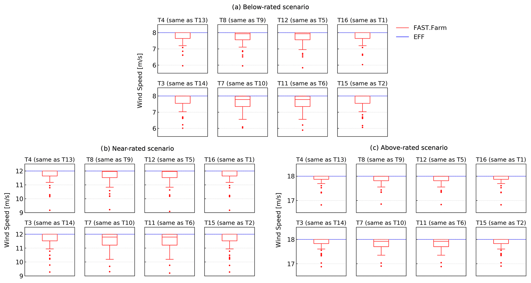
Figure 12 Mean wind speed (m s⁻¹) at each wind turbine in the farm for each wind speed scenario. The FAST.Farm results are given in terms of boxplots and outliers, with 72 seed-averaged values (one for each wind direction) included in each distribution. The effective turbulence model (EFF) results are given as the horizontal line, which is constant for all wind turbines and represents the undisturbed wind speed. For brevity, only the top half of the wind farm is shown. Results are symmetric for the bottom half.

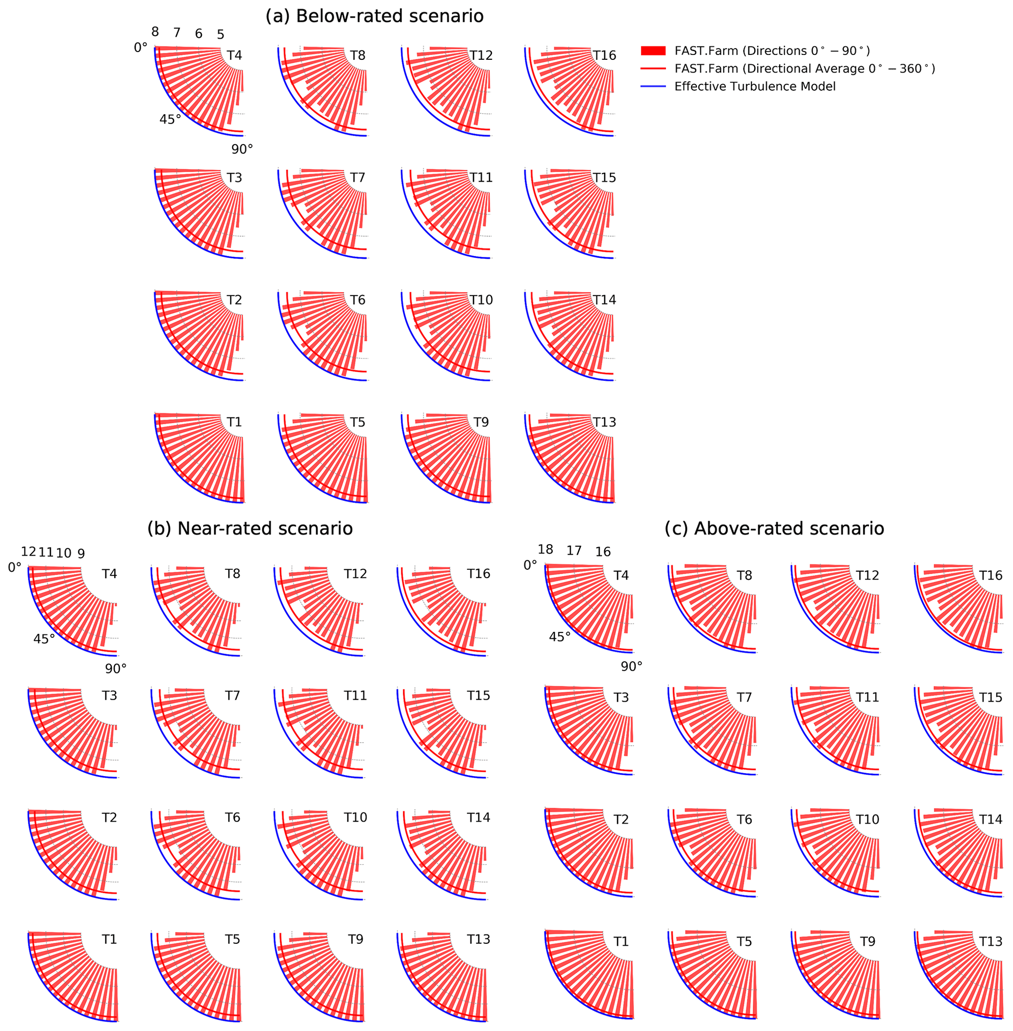
Figure 13 Mean hub-height wind speed (m s⁻¹) at each wind turbine in the farm for each wind speed scenario. The FAST.Farm bars represent seed-averaged results for wind directions 0–90^∘, while the solid line is the directional average for wind directions 0–360^∘. The effective turbulence model (EFF) line is constant for all subplots due to the lack of wake wind speed deficits in the EFF modeling approach.

3.2 Wind turbine loads

The analysis performed up to now indicated overall higher mean turbulence with wakes for the EFF compared to FAST.Farm. Based on this result, it would be reasonable to expect that the EFF would consistently predict higher load variability than FAST.Farm. To assess this hypothesis, we consider the distributions of load standard deviations (Fig. 14), a quantity that we use as a proxy for fatigue loads. The standard deviations are computed over 10 min of load time series for each wind turbine, seed, and wind farm orientation. We see that the median values of the load standard deviations are indeed generally higher for EFF than FAST.Farm, as signaled by the mostly positive percent values above the distribution pairs. These percent values represent the difference between the median standard deviation for FAST.Farm and the EFF. Differences higher than 5 % are shown in bold, revealing that the biggest discrepancies are for blade-root out-of-plane bending moment, tower-base fore-aft moment, tower-top side-side moment, and torque. Whenever the percent difference is negative (i.e., the FAST.Farm median standard deviation is higher), the difference is low (i.e., < 3 %). Another obvious takeaway from Fig. 14 is the much larger spread of the FAST.Farm distribution with long upper and lower tails. This is due to the wind direction effects, which are explicitly present in the FAST.Farm results and only implicitly included in the EFF calculations as well as in the spatial variation of turbulence in the FAST.Farm results.

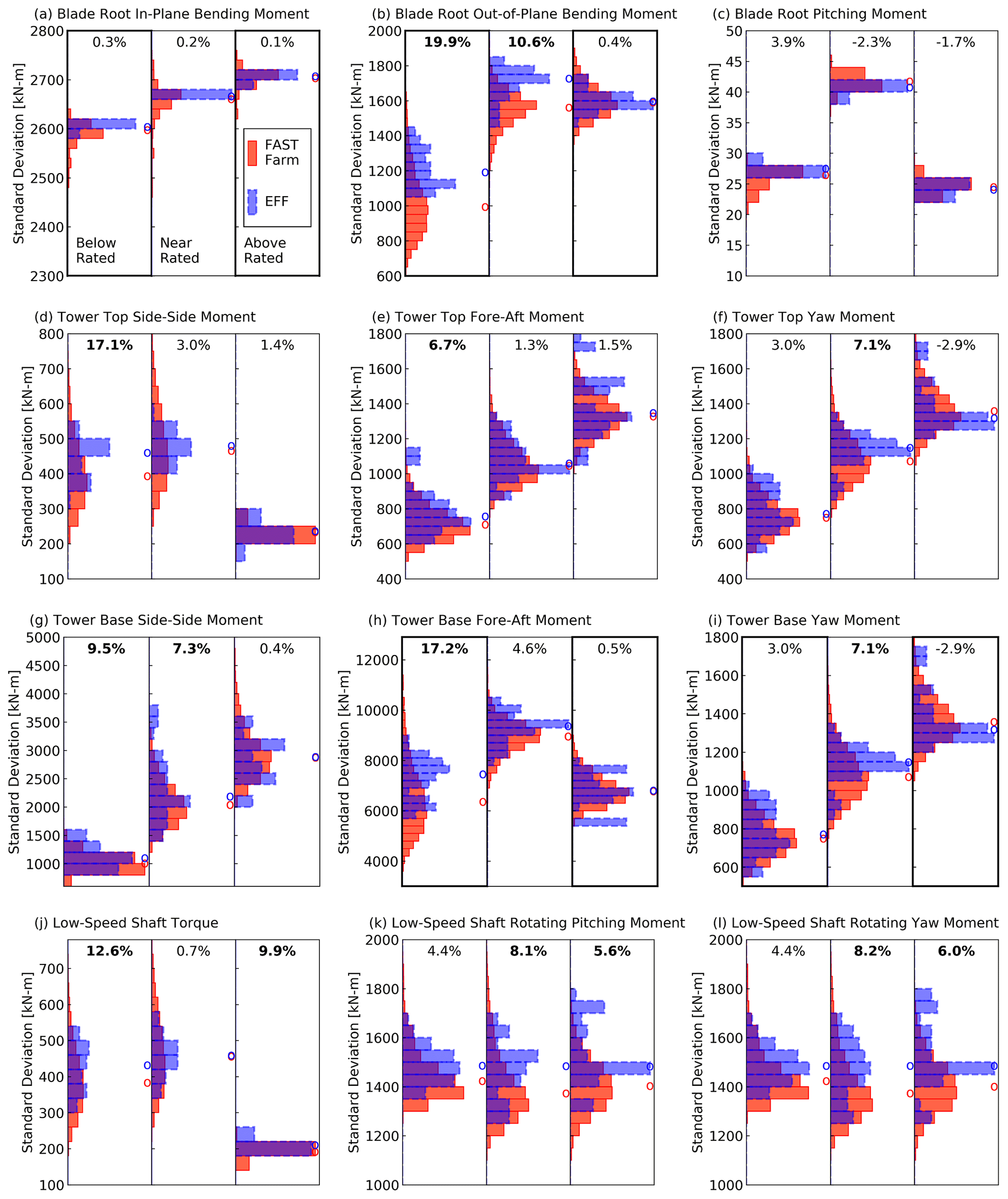
Figure 14 Distribution of load standard deviations (σ). Each subpanel gives the distributions for FAST.Farm (11 520 points: 16 wind turbines, 10 seeds, 72 wind directions) and the effective turbulence model (160 points: 16 wind turbines, 10 seeds). The percent values above each pair of distributions represent the difference in median standard deviation between both modeling approaches: $\left(\langle {\mathit{\sigma }}_{\mathrm{EFF}}\rangle -\langle {\mathit{\sigma }}_{\mathrm{FASTFarm}}\rangle \right)/\langle {\mathit{\sigma }}_{\mathrm{FASTFarm}}\rangle \times \mathrm{100}\mathit{\%}$. The thick borders mark quantities for which power spectra are provided in Figs. 15 and 16.

The statistical analysis discussed above quantified the differences in load fluctuations between the two modeling approaches. Next, we consider load power spectra to determine whether these differences in standard deviation are concentrated to a particular frequency range. We focus on blade-root and tower-base moments and consider the below-rated and above-rated scenarios (Figs. 15 and 16). We choose the below-rated scenario due to the importance of wakes at these lower wind speeds and the above-rated scenario because high winds are usually the main drivers of fatigue. We choose blade root and tower base for having higher load variability magnitudes. At the blade root (Fig. 15), we see that the in-plane moment differences are concentrated at the blade-passing frequency 1P (∼0.14 Hz below rated and 0.2 Hz above rated). For the out-of-plane bending moment, the large difference in distribution spread and median observed at below-rated wind speed in Fig. 14b is concentrated primarily at the low-frequency end of the spectrum followed by 1P. Above rated wind speed, the differences in out-of-plane moment are also largest at the low-frequency end, with small differences also observed for 1P, 2P, and 3P. At the tower base (Fig. 16), we saw larger fore-aft moment standard deviation differences below rated than above rated (Fig. 14h). At first glance, the spectra seem to indicate the opposite due to the large differences at low frequencies seen in Fig. 16b. However, the differences are indeed larger below rated than above rated, as can be noted by the different orders of magnitude in the vertical axis between Fig. 16a and b. For both scenarios, the spectra reveal that the tower fore-aft moment differences are concentrated at the low-frequency end of the spectrum with small differences near the first tower natural frequency (∼0.32 Hz) and 3P. The yaw moment spectral power differences are driven primarily by low frequencies followed by 3P.

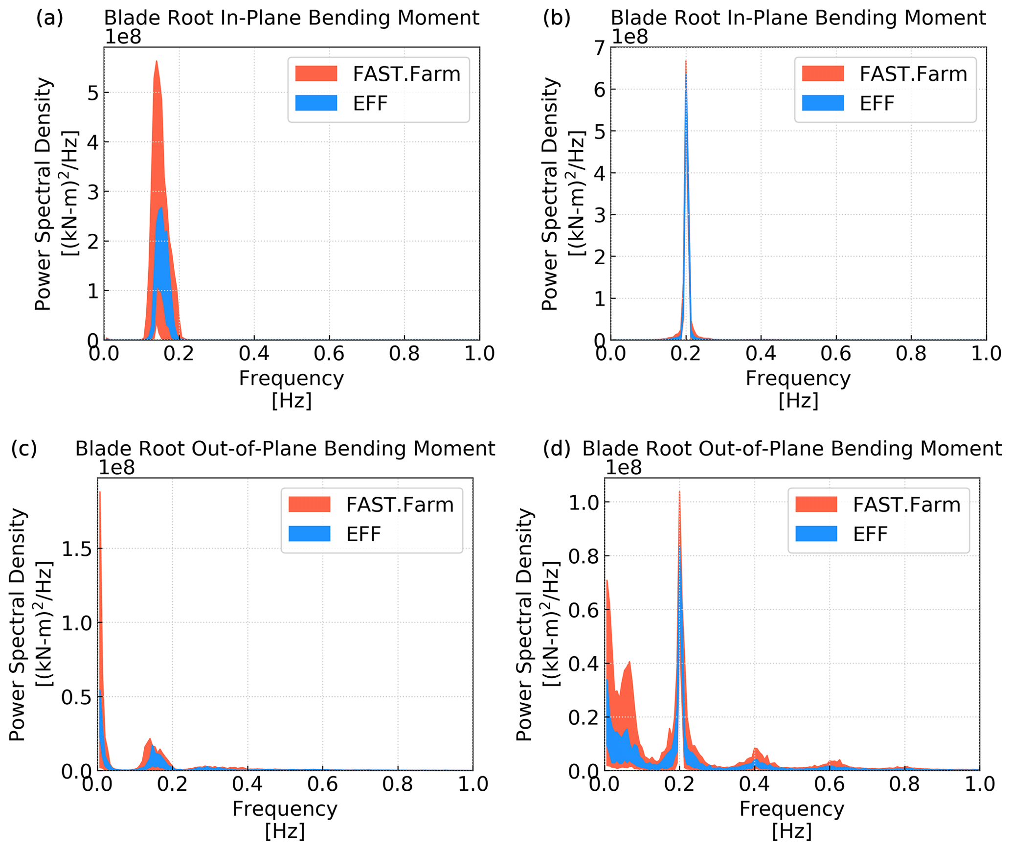
Figure 15 Power spectral density for the (a, b) blade-root in-plane and (c, d) out-of-plane moments for the (a, c) below-rated and (b, d) above-rated wind speed scenarios. The spectra are first obtained for each 10 min time series using Welch's method and a Hanning window on 150 s segments. Next, range (minimum to maximum) of spectral power is plotted at each frequency.

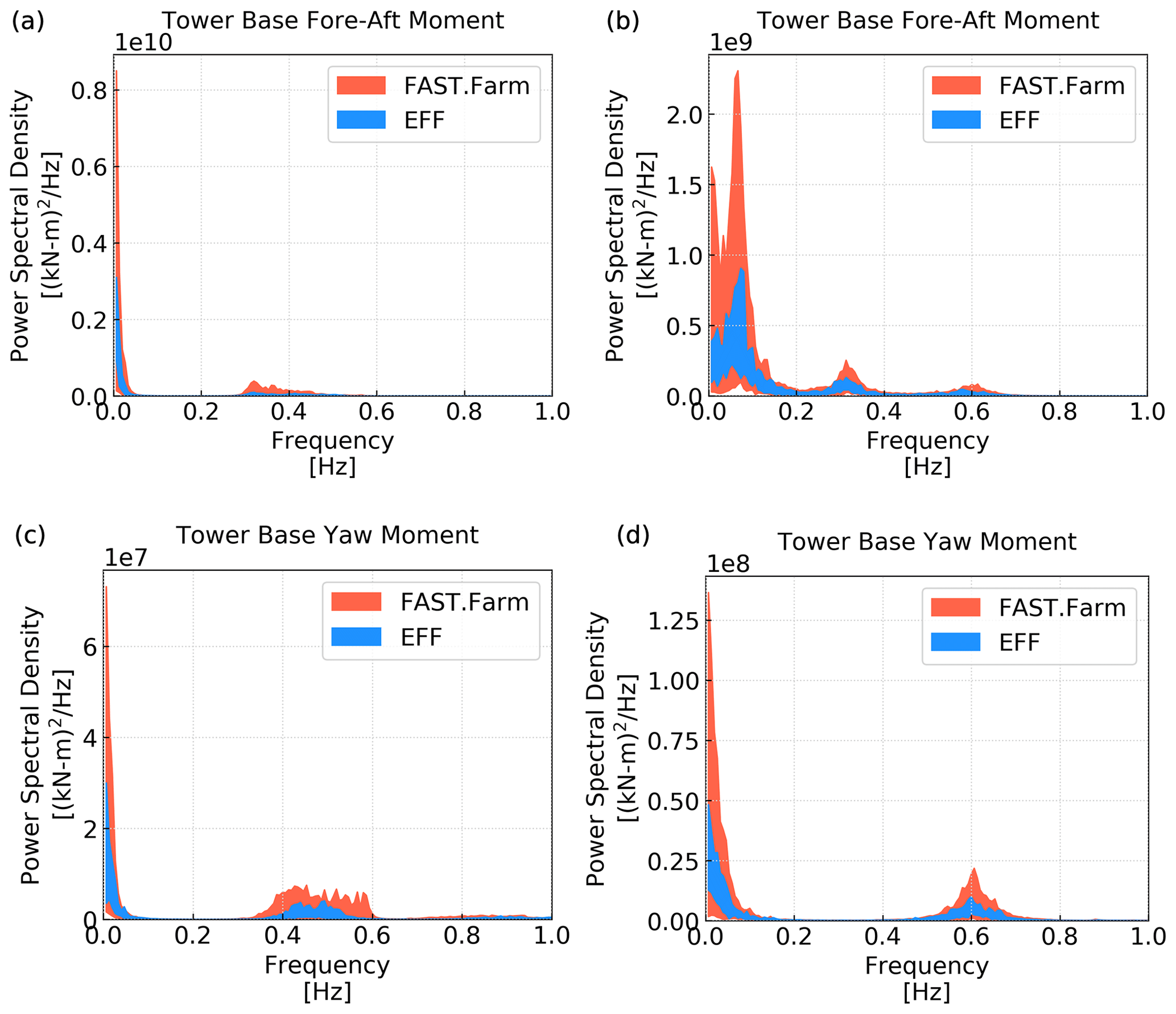
Figure 16 Power spectral density for the (a, b) tower-base fore-aft and (c, d) yaw moments for the (a, c) below-rated and (b, d) above-rated wind speed scenarios. The spectra are first obtained for each 10 min time series using Welch's method and a Hanning window on 150 s segments. Next, range (minimum to maximum) of spectral power is plotted at each frequency.

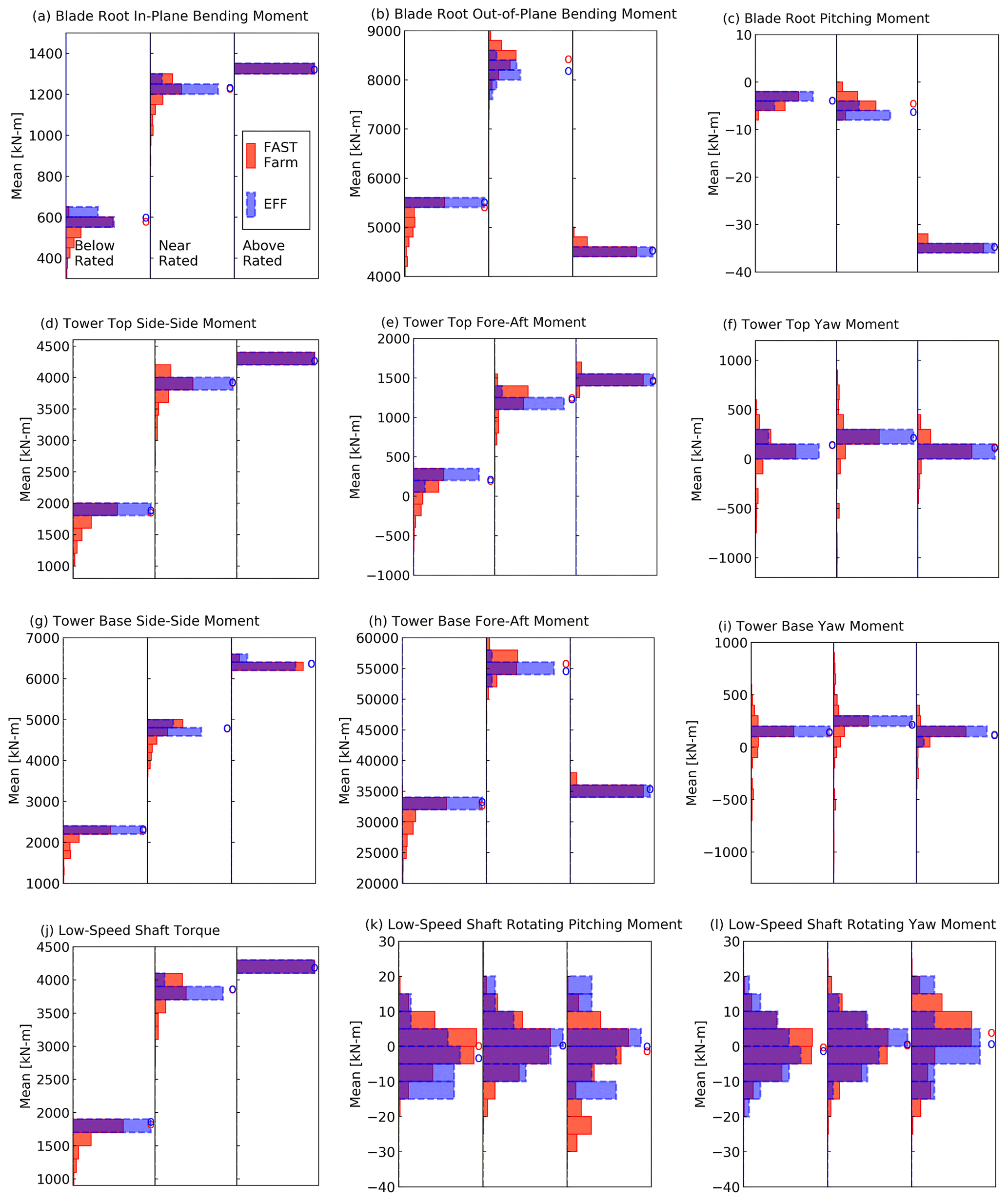
Figure 17 Distribution of 10 min means (μ) for loads. Each subpanel gives the distributions for FAST.Farm (11 520 points: 16 wind turbines, 10 seeds, 72 wind directions) and the effective turbulence model (160 points: 16 wind turbines, 10 seeds).

In addition to load fluctuations, we now compare the mean load values between the two modeling approaches. Recall that the vertical shear profile is the same for the two methods: a power law with a 0.2 exponent. Therefore, the main difference in the mean flow fields is the wind speed magnitude: at a fixed height, it is constant for EFF and variable for FAST.Farm depending on the wake presence and strength. As shown in Fig. 12, the mean wind speed value in FAST.Farm is close to the freestream value, but the spread of the distribution is large with a long tail toward lower wind speeds. A similar result is seen for the mean loads (Fig. 17): the median values (marked by circles above the bars in each subplot) are close for both methods, but FAST.Farm 10 min means are much more widely distributed than those of the EFF. The FAST.Farm distributions present a large tail toward low values for all load quantities that are positive scalars. For the load signals that can take on positive and negative values, the tails extend to both sides of the median. Overall, the differences between the two modeling approaches are less pronounced for the 10 min mean loads than they were for the 10 min standard deviations of loads.

4 Summary and conclusions

The work presented here compares wind farm loads simulated with two different modeling approaches: the effective turbulence model and the dynamic wake meandering model as implemented in FAST.Farm. Both simulation strategies are provided as viable alternatives in the international standard for wind turbine design (International Electrotechnical Commission, 2019). The results from our comparison are summarized below in an effort to support intentional and informed decision making by modeling experts working with wind turbine and wind farm design.

For all cases considered, the EFF wind farm turbulence levels are consistently higher than the FAST.Farm medians computed across all wind directions (0–360^∘ in 5^∘ increments). However large, these EFF turbulence levels are still always within the directional distribution of FAST.Farm values. When comparing EFF to the FAST.Farm medians, turbulence intensity differences range between 0.2 % and 2.7 %, with FAST.Farm being lower. When comparing EFF to the FAST.Farm maximum wind farm turbulence levels, differences reach up to 8.6 %, with FAST.Farm being higher. The turbulence differences between both approaches are larger when the wake influence is strongest, which applies to wind turbines in the center of the farm and those in rows with tighter spacing. Wake-added turbulence, which is not accounted for in the FAST.Farm version used here, is not expected to have substantial effects on the results because the ambient turbulence levels considered here are already high (13.1 %–16.5 %). A previous study (Shaler and Jonkman, 2021) found that FAST.Farm matches large-eddy simulation results well at high turbulence levels (i.e., greater than 10 %) with differences seen at low turbulence levels (i.e., lower than 6 %). On average, our results agree with Argyle et al. (2018); Reinwardt et al. (2018), who compared the EFF to measurements and DWM predictions and found EFF to overestimate turbulence levels. However, it is important to also note that the FAST.Farm wind farm turbulence is widely distributed and can, for certain wind directions and wind speeds, be substantially higher than that of the EFF. In terms of wind speeds, EFF compares well to the FAST.Farm directional median but can differ by up to 3 m s⁻¹ when the FAST.Farm directional distribution extremes are considered. These large wind speed differences are due to the lack of wake deficits in the EFF formulation.

These flow field differences directly affect the load results. In terms of load means, the results are similar to the wind farm wind speed comparisons: EFF compares well to the FAST.Farm directional median but produces a narrower distribution of load means than FAST.Farm. The wider distribution in FAST.Farm is expected because the wakes are being modeled explicitly in the wind farm simulations, leading to different mean loads depending on the location of the wind turbine and the wind direction. For most signals (in-plane loads, out-of-plane loads and torque) the FAST.Farm distribution shows a tail towards lower values, which is likely to lower the fatigue loads because most materials can better withstand fatigue cycles at lower mean loads than they can when the mean loads are larger (based on the Goodman correction). In terms of load standard deviations, the EFF medians are overall higher than those of FAST.Farm, with differences being largest for the blade-root (∼20 %) and tower-base (∼17 %) fore-aft moment below-rated wind speed. The load spectra for these quantities show the largest differences at low frequencies, indicating that they are driven by the inflow. An example of a contrasting result is the in-plane blade-root moment for which differences are concentrated in the first blade-passing harmonic. Our results indicate larger differences for blade root than for the tower, unlike the results of Reinwardt et al. (2018) and Schmidt et al. (2011b). In terms of the magnitude of these differences, it is hard to do a one-to-one comparison of our results to previous studies due to the differences in simulation setups and analysis methods. However, we can say that our results broadly agree with Schmidt et al. (2011b), who found differences on the order of 10 % for blade flap-wise moments and 20 % for tower-base moments when comparing the EFF to a DWM implementation coupled to Bladed for the load calculations. The tower yaw moment, which was highlighted in a previous EFF–DWM comparison for being particularly sensitive to wind direction (Thomsen et al., 2007), remained within ∼7 % for the two modeling approaches.

Our analysis considered freestream turbulence, wind farm turbulence, load standard deviations, spectra, and means. It is clear from our results that substantial differences between both modeling approaches are already present at the very beginning of the simulation chain, before wakes are computed. As expected, these differences persist through to the load results. The message is clear: on average, the EFF predicts higher turbulence and load variability but grossly misses the wide distribution of turbulence and load levels that is found in wind farms, not only due to wind direction variations with respect to the farm layout, but also due to the spatial variability of turbulence itself even before wakes are taken into account.

The computational cost for running FAST.Farm instead of the EFF was 14 times higher for the inflow and 7 times higher for the wake and load simulations. Having said that, none of the simulations performed for this work required more than one computer node. Therefore, the added cost of running FAST.Farm is still arguably low and is not expected to hinder any future changes toward higher-fidelity design simulations.

Considering the largest differences we found (approximately 3 m s⁻¹ in 10 min mean wind speed, 7 % in 10 min turbulence intensity, 20 % in medians of 10 min load standard deviations) and the arguably low increase in computational expense, we suggest that the wind industry seriously considers moving toward validated, higher-fidelity simulation tools such as FAST.Farm or other equivalent DWM approaches. By updating the wind turbine design paradigm, we have the potential to better optimize wind turbine designs or selections for conditions local to their installation site within a farm. In addition, this change might prevent large unnecessary costs associated with overdesigning wind turbine components at sites in which design is driven by fatigue.

To complement the results presented here, future studies should focus on lifetime fatigue analysis and consider other wind turbine archetypes, realistic wind farm layouts, and nonuniform wind direction distributions. Inflow, turbine response, and wake measurements from a utility-scale wind farm would be valuable additions to the results we present. Finally, to support the adoption of higher-fidelity tools in design applications, we suggest that a standard procedure be developed through which DWM models can be applied in design and site suitability analyses.

Appendix A: FAST.Farm simulation setup

The FAST.Farm parameters common to all simulations performed in this work are as follows:

• type of inflow (Mod_AmbWind): three (i.e., separate synthetic farm-wide and turbine-specific inflow domains)

• time step for domains specific to wind turbines (DT_High): 0.1 s

• number of planes used in wake calculations (NumPlanes): 175

• number of radii in the radial finite-difference grid (NumRadii): 75

• radial increment of radial finite-difference grid (dr): 5 m

• vertical start of domains specific to wind turbines (Z0_High): 0.01 m

• lateral and vertical start of farm-wide inflow domain (Y0_Low Z0_Low): −2325 and 0.01 m.

The FAST.Farm parameters common to all wind farm orientations and turbulent seeds but varying for the three inflow scenarios are given below. The three numbers provided for each quantity are given for the below-, near-, and above-rated scenarios, respectively.

• time step and simulation duration:

  • –

    simulation time (TMax): 1100, 1000, and 900 s (only the last 600 s are used in the analysis, allowing for a spinup of 500, 400, and 300 s for each inflow scenario)

  • time step for wind farm domain (DT): 3, 2, and 1.3 s

• setup of the 16 domains specific to each wind turbine:

  • –

    number of points in wind turbine domain (NX_High, NY_High, NZ_High): (33, 31, 34), (33, 31, 34), (29, 31, 34)

  • –

    spatial resolution along x, y, and z in wind turbine domain (dX_High, dY_High, dZ_High): (4.8, 5, 5) m, (4.8, 5, 5) m, and (5.4,5,5) m

• setup of the farm-wide inflow domain:

  • –

    number of points along y and z in wind farm domain (NY_Low, NZ_Low): (310, 29), (232, 22), and (155, 15).

  • –

    spatial resolution along x, y, and z in wind farm domain (dX_Low, dY_Low, dZ_Low): (12.325, 15, 15) m, (18.488, 20, 20) m, and (27.720, 30, 30) m.

Appendix B: TurbSim simulation setup

When generating the farm-wide inflows for FAST.Farm, the only varying TurbSim parameters across inflow scenarios are IECTurbc (set to I_mid,des, Table 2), URef (set to V_hub), and NumGrid_Z and NumGrid_Y (Table B1). The TurbSim parameters common to all farm-wide simulations are as follows:

• time series length (AnalysisTime): 600 s

• time step (TimeStep): 0.1 s

• grid height (GridHeight): 420 m

• grid width (GridWidth): 4 650 m

• assumed hub height (HubHt): 210 m (while TurbSim refers to this as HubHt, we refer to it as the vertical center of the grid z_mid to avoid confusion with the wind turbine hub height z_hub)

• vertical wind shear (WindProfileType and PLExp): 0.2 power-law exponent

• turbulence model (TurbModel): Kaimal spectrum (IECKAI)

• spatial coherence model (SCMod1, SCMod2, SCMod3): IEC

• spatial coherence parameters (IncDec1=IncDec2=IncDec3): (12.0, 0.0003527) is based on International Electrotechnical Commission (2019) recommendations with a=12 and $b=\mathrm{0.12}/(\mathrm{8.1}\cdot {\mathrm{\Lambda }}_{\mathrm{1}})$, where Λ₁=42 m

• coherence exponent (CohExp): 0.0.

Table B1 Farm-wide inflow domain TurbSim parameters that varied across inflow scenarios: lateral grid size (GridWidth), number of points along vertical (NumGrid_Z) and lateral (NumGrid_Y) dimensions, and spatial resolution of generated flow fields vertically $dz=\mathtt{\text{GridHeight}}/(\mathtt{\text{NumGrid\_Z}}-\mathrm{1})$ and laterally d$y=\mathtt{\text{GridWidth}}/(\mathtt{\text{NumGrid\_Y}}-\mathrm{1})$.

For the inflow generation specific to each wind turbine, the only varying TurbSim parameter across inflow scenarios is URef (set to V_hub). The TurbSim parameters common to all wind turbine simulations but different from the farm-wide domain simulations are as follows:

• grid height (GridHeight): 165 m

• grid width (GridWidth): 150 m

• number of points vertically (NumGrid_Z): 34

• number of points horizontally (NumGrid_Y): 31

• vertical resolution, GridHeight/(NumGrid_Z-1): 5 m

• horizontal resolution, GridWidth/(NumGrid_Y-1): 5 m

• turbulence model (TurbModel): constrained turbulence (TIMESR).

The parameters AnalysisTime, TimeStep, WindProfileType, PLExp, IncDec1, IncDec2, IncDec3, and CohExp match those used for the farm-domain simulations.