Increased power gains from wake steering control using preview wind direction information

Yaw controllers typically rely on measurements taken at the wind turbine, resulting in a slow reaction to wind direction changes and subsequent power losses due to misalignments. Delayed yaw action is especially problematic in wake steering operation because it can result in power losses when the yaw misalignment angle deviates from the intended one due to a changing wind direction. This study explores the use of preview wind direction information for wake steering control in a two-turbine setup with a wind speed in the partial load range. For these conditions and a simple yaw controller, results from an engineering model identify an optimum preview time of 90 s. These results are validated by forcing wind direction changes in a large-eddy simulation model. For a set of six simulations with large wind direction changes, the average power gain from wake steering increases from only 0.44 % to 1.32 %. For a second set of six simulations with smaller wind direction changes, the average power gain from wake steering increases from 1.24 % to 1.85 %. Low-frequency fluctuations are shown to have a larger impact on the performance of wake steering and the effectiveness of preview control, in particular, than high-frequency fluctuations. From these results, it is concluded that the benefit of preview wind direction control for wake steering is substantial, making it a topic worth pursuing in future work.

1 Introduction

To support the energy transition, it is important to maximize the value of the renewable energy portfolio. On the one hand, this includes minimizing the costs of installation and maintenance; on the other hand, this means maximizing the power yield. Focusing on wind energy, wind farm control to mitigate wake effects has received considerable attention in recent years (Meyers et al., 2022). Additionally, short-term forecasting of the wind speed and direction can be used to adapt the turbine for approaching changes; hereafter, this is called preview control (PC), as opposed to traditional standard control (SC) using measurements at the turbine.

PC can be used to reduce the occurrence of suboptimal blade pitch angles and turbine misalignment, two aspects that result in power losses and increased loads (Scholbrock et al., 2016). Furthermore, operators can use the forecasts to support grid stability and reduce curtailment (Bird et al., 2016). Downstream turbines can use information from turbines further upstream (Rott et al., 2020), or remote sensing techniques (lidar-assisted control) can be used (e.g., Theuer et al., 2020; Würth et al., 2019). Many studies have investigated the application of preview wind speed information in turbine control, a few of which are discussed in the following. Torque control to improve its aerodynamic efficiency is observed to achieve very small power gains, but it drastically increases the turbine's loads (Schlipf et al., 2011; Wang et al., 2013). However, pitch control significantly reduces the loads with a minimum change in generated power (Dunne et al., 2011; Bossanyi et al., 2014). Combinations of the two have shown promising results in terms of both reducing the loads and increasing the power (Schlipf et al., 2013; Schlipf and Cheng, 2014).

On the contrary, remote sensing techniques to improve the turbine's yaw control are relatively rare and are usually only done to help calibrate the nacelle's wind vane (e.g., Fleming et al., 2014; Scholbrock et al., 2015). This is interesting, as some studies have reported potential power gains from reduced yaw misalignment when using preview information. Spencer et al. (2011) modeled perfect wind direction prediction to reduce the yaw misalignment of a single turbine, resulting in a power gain of 0.5 % and a reduction in fatigue loads. Using a weighted average of wind direction measurements from upstream turbines, Bossanyi (2019) found a 0.2 % power increase and a 24 % reduction in yaw travel for a wind farm in a 30 min simulation. Similarly, Sinner et al. (2021) averaged wind direction signals of neighboring turbines to obtain a smoother wind direction signal. They demonstrated that this results in power gains and yaw travel reductions for both greedy and wake steering operations, but using preview information did not yield significant results. In light of the controller lag observed in a wake steering experiment reported in Fleming et al. (2019), Simley et al. (2021b) employed the FLOw Redirection and Induction in Steady State (FLORIS) simulation tool (NREL, 2022) to compare preview control using wind direction information to standard control for a turbine pair in wake steering operation. Using an optimal preview time of 90 s, their results demonstrate that the power gain of 5.8 % achieved with SC wake steering increases to 8.9 % when PC is enabled. However, this analysis uses perfect preview information, and no improvement was found with realistic measurement accuracy. Howland et al. (2022) simulated a diurnal cycle with time-varying wind speed, wind direction, and atmospheric stability in a large-eddy simulation (LES) model. Using a simple forecasting method based on linear regression of past data, they demonstrated that in wake steering operation, PC's power production is slightly increased compared to that of SC.

Although it intuitively makes sense that PC turbines anticipating an approaching wind direction change yield more power than SC turbines, it is a relatively unexplored topic. PC is expected to be especially beneficial in wake steering operation because it could limit erroneous wake steering, which is when wake steering results in power losses compared to greedy control (e.g., Doekemeijer et al., 2021). The magnitude of potential power gains is unknown, but they should be substantial to make preview control worth pursuing in future work.

The objective of this paper is to demonstrate the benefit of using preview wind direction observations for wake steering purposes to further increase power production. Preview information is obtained from a virtual met mast located upstream, as developing a more sophisticated wind direction forecasting technique was considered out of scope. This objective comprises three components: (1) to develop a simple engineering model to obtain estimates of the expected power gain and optimal preview time; (2) to validate the findings of the engineering model with results from large-eddy simulations; and (3) to identify the characteristics of the wind direction signal that benefit from preview control the most.

2 Turbine yaw controller

This section describes the turbine yaw controller used in this study. It covers how the controller functions in greedy and wake steering operations, as well as how preview control is handled. The turbine pair simulated in this study consisted of two NREL 5 MW turbines with a hub height of 90 m and a rotor diameter D=126 m (Jonkman et al., 2009). While the upstream turbine could operate in greedy or wake steering control, the downstream turbine always operated in greedy yaw control.

2.1 Greedy

The turbine controller used a 60 s moving average of wind direction observations $\stackrel{\mathrm{‾}}{\mathit{\delta }}$ and turbine orientation γ to determine the yaw misalignment angle $\stackrel{\mathrm{‾}}{\mathit{\varphi }}$ of the turbine with the inflow wind direction:

$$\begin{array}{}\text{(1)}& \stackrel{\mathrm{‾}}{\mathit{\varphi }}=\mathit{\gamma }-\stackrel{\mathrm{‾}}{\mathit{\delta }}.\end{array}$$

Once $\left|\stackrel{\mathrm{‾}}{\mathit{\varphi }}\right|$ exceeded a preset limit of 7.5^∘, the turbine corrected its orientation at 0.3^∘ s⁻¹, as is standard for the NREL 5 MW turbine, until $\left|\stackrel{\mathrm{‾}}{\mathit{\varphi }}\right|\le \mathrm{0.15}$^∘ was reached. This check was performed every second, except during and the first minute after a yaw maneuver, to eliminate measurements disturbed due to the rotating nacelle.

2.2 Wake steering

To implement wake steering, existing controllers are typically adapted to include an intended target yaw misalignment ϕ_t. In this study, a positive misalignment was defined as a clockwise rotation of the turbine when looking from above. Because of the intentional misalignment, an effective yaw angle $\stackrel{\mathrm{‾}}{{\mathit{\varphi }}_{\mathrm{e}}}$ was determined:

$$\begin{array}{}\text{(2)}& \stackrel{\mathrm{‾}}{{\mathit{\varphi }}_{\mathrm{e}}}=\mathit{\gamma }-\stackrel{\mathrm{‾}}{\mathit{\delta }}-{\mathit{\varphi }}_{\mathrm{t}},\end{array}$$

which triggered a yaw maneuver when $\left|\stackrel{\mathrm{‾}}{{\mathit{\varphi }}_{\mathrm{e}}}\right|$ exceeded 7.5^∘. ϕ_t was determined using a lookup table (LUT) that contained the power-maximizing yaw misalignment angles as a function of inflow conditions. The LUT was developed based on the Data-driven wAke steeRing surrogaTe model (DART) introduced in Sengers et al. (2022). This wake model uses a set of only linear equations ($\mathbf{Y}=\mathbf{X}\times \mathbf{B}$) to estimate wake characteristics Y (e.g., deficit, center position) from the input variables X (e.g., yaw angle, shear exponent, thrust coefficient). The model coefficients B are found by a regression analysis with reference data. The wake characteristics can consequently be used to generate a vertical cross-section of the streamwise wind speed component to estimate the available power at a virtual wind turbine at a downstream position. Based on the results described in Sengers et al. (2022), the set of (ϕ_t, $\stackrel{\mathrm{‾}}{\mathit{\delta }\mathit{\alpha }}$ and C_T), in which $\stackrel{\mathrm{‾}}{\mathit{\delta }\mathit{\alpha }}$ is the 60 s moving-averaged vertical wind veer over the rotor area, were used as input variables. The thrust coefficient C_T was estimated as a function of ϕ_t:

$$\begin{array}{}\text{(3)}& C_{\mathrm{T}}=C_{\mathrm{T},{\mathit{\varphi }}_{\mathrm{0}}}{\cos }^{\mathrm{1.28}}\left({\mathit{\varphi }}_{\mathrm{t}}\right),\end{array}$$

in which $C_{\mathrm{T},{\mathit{\varphi }}_{\mathrm{0}}}$ is the turbine's thrust coefficient at $\mathit{\varphi }=\mathrm{0}{}^{\circ }$. This is analogous to how the power coefficient is typically corrected for the yaw angle in wake modeling; see also Eq. (5). The exponent 1.28 was determined using LES data from Sengers et al. (2022). The same LES results were used for training to obtain the model coefficients B.

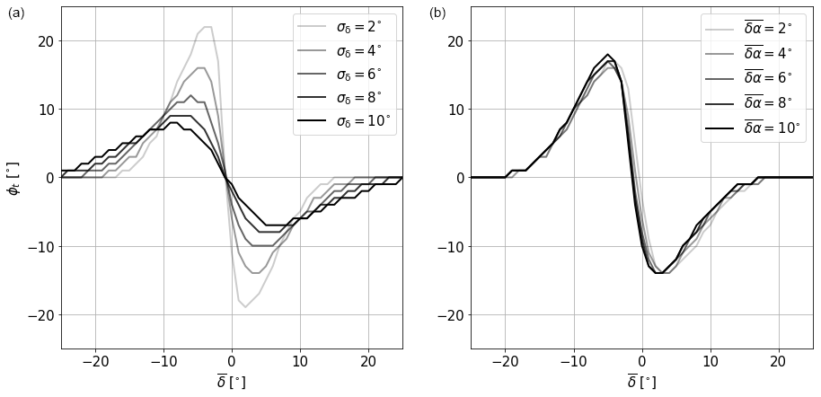
Figure 1 Target yaw misalignment ϕ_t as a function of the 60 s averaged wind direction $\stackrel{\mathrm{‾}}{\mathit{\delta }}$ for a changing wind direction standard deviation of σ_δ with a wind veer $\stackrel{\mathrm{‾}}{\mathit{\delta }\mathit{\alpha }}=\mathrm{4}$^∘ (a) and for a changing $\stackrel{\mathrm{‾}}{\mathit{\delta }\mathit{\alpha }}$ with σ_δ= 4^∘ (b). A turbine spacing of 6 D is assumed and $\stackrel{\mathrm{‾}}{\mathit{\delta }}=\mathrm{0}{}^{\circ }$ indicates the wind direction where the turbine pair is aligned.

Uncertainty is typically included in the form of adding discretized wind direction variability bins to the LUT (Rott et al., 2018; Simley et al., 2020). Rather than for the mean wind direction only, the optimal yaw misalignment is computed for a distribution of wind directions – typically a Gaussian distribution with standard deviation σ_δ around a mean $\stackrel{\mathrm{‾}}{\mathit{\delta }}$. This uncertainty parameter σ_δ is affected by the wind direction variability as well as the accuracy of the measurement devices, although the latter is not considered in the current work. This results in a more conservative controller setting when the uncertainty is high, mitigating erroneous steering but also resulting in a lower achievable power gain. On average, however, this results in a higher gain than if a more aggressive controller setting was used. In the current study, the target yaw angle was therefore determined from the LUT as a function ${\mathit{\varphi }}_{\mathrm{t}}\left(\stackrel{\mathrm{‾}}{\mathit{\delta }},\stackrel{\mathrm{‾}}{\mathit{\delta }\mathit{\alpha }},{\mathit{\sigma }}_{\mathit{\delta }}\right)$. For clarity, however, this notation is omitted in the remainder of the present work. Referring back to Eq. (2), this indicates that not only could a change in $\stackrel{\mathrm{‾}}{\mathit{\delta }}$ cause $\left|{\mathit{\varphi }}_{\mathrm{e}}\right|$ to exceed 7.5^∘ but also that a change in $\stackrel{\mathrm{‾}}{\mathit{\delta }\mathit{\alpha }}$ or σ_δ could initiate a yaw maneuver.

Figure 1 illustrates the ϕ_t suggested by the LUT as a function of $\stackrel{\mathrm{‾}}{\mathit{\delta }}$. Figure 1a shows that with increasing uncertainty (higher σ_δ), the controller setting becomes more conservative: for σ_δ= 2^∘, the maximum ϕ_t is 22^∘, whereas, when σ_δ= 10^∘, the controller settings have a maximum of ϕ_t of 8^∘, corresponding to the logic discussed before. Figure 1b illustrates that the aggressiveness of the controller setting does not really depend on $\stackrel{\mathrm{‾}}{\mathit{\delta }\mathit{\alpha }}$, but the controller switches from positive to negative ϕ_t at a different $\stackrel{\mathrm{‾}}{\mathit{\delta }}$. Wind veer inherently deflects the wake due to a crosswise force pointing toward the right above hub height and to the left below hub height (when looking downstream). Since the wind speed is higher above hub height, the rotor equivalent wake deficit is deflected to the right. With increasing veer, this effect becomes stronger and the wind direction under which a full wake situation occurs (typically the crossover point in the LUT) moves to the left (a more negative $\stackrel{\mathrm{‾}}{\mathit{\delta }}$).

3 Simulation environment

3.1 Engineering model

A simple engineering model is developed to estimate the power gain and optimal preview time for a given time series of the wind direction. Assuming a constant wind speed, it computes the power yield of a turbine pair as a function of the wind direction only.

The instantaneous power is computed with

$$\begin{array}{}\text{(4)}& P=\mathrm{0.5}\mathit{\rho }{C}_{\mathrm{P}}\mathit{\pi }{R}^{\mathrm{2}}{U}_{\mathrm{eq}}^{\mathrm{3}},\end{array}$$

in which ρ is the air density, R is the turbine radius and U_eq is the rotor equivalent wind speed. C_P is the turbine’s power coefficient corrected for the yaw misalignment ϕ:

$$\begin{array}{}\text{(5)}& C_{\mathrm{P}}=C_{\mathrm{P},{\mathit{\varphi }}_{\mathrm{0}}}{\cos }^{\mathrm{1.89}}\left(\mathit{\varphi }\right),\end{array}$$

which is analogous to Eq. (3). The exponent 1.89 (referred to as P_p in the literature; e.g., Howland et al. (2020)) is again based on LES data from Sengers et al. (2022). A low-pass filter is applied to the wind direction time series using a cutoff frequency of 0.0037 Hz, as proposed in Simley et al. (2020). For each point in the low-pass-filtered wind direction time series δ_lp(t), the power generated by the upstream turbine can be estimated as described in the following:

1. Calculate the yaw misalignment ϕ_up from the current turbine orientation γ and the low-pass-filtered wind direction at time t: ${\mathit{\varphi }}_{\mathrm{up}}={\mathit{\gamma }}_{\mathrm{up}}-{\mathit{\delta }}_{\mathrm{lp}}\left(t\right)$.

2. Calculate C_P,up according to Eq. (5) using ϕ_up.

3. Calculate P_up using Eq. (4) with C_P,up and a constant U_eq,up.

To estimate the power of the downstream turbine, a wake model needs to be employed. In this study, again, DART with ϕ, $\stackrel{\mathrm{‾}}{\mathit{\delta }\mathit{\alpha }}$ and C_T as input variables is used to make these estimations. A constant veer of $\stackrel{\mathrm{‾}}{\mathit{\delta }\mathit{\alpha }}$ (see Sect. 3.2.1) is assumed.

• 4.

  Calculate ${\mathit{\varphi }}_{\mathrm{dn}}={\mathit{\gamma }}_{\mathrm{dn}}-{\mathit{\delta }}_{\mathrm{lp}}(t-\mathrm{\Delta }T)$. Here, δ_lp(t) is time-shifted by $\mathrm{\Delta }T=x/U_{\mathrm{h}}$, where x is the turbine spacing and U_h is the wind speed at hub height.

• 5.

  Calculate C_T,up of the upstream turbine with Eq. (3) using ϕ_up.

• 6.

  Model wake characteristics with DART, using (ϕ_up, $\stackrel{\mathrm{‾}}{\mathit{\delta }\mathit{\alpha }}$ and C_T,up) as input parameters.

• 7.

  Move the wake position by $\mathrm{\Delta }y=\sin \left({\mathit{\delta }}_{\mathrm{lp}}\right(\mathrm{t}-\mathrm{\Delta }\mathrm{T}\left)\right)\cdot x$, in which δ_lp(t−ΔT) is the time-shifted low-pass-filtered wind direction and x is the turbine spacing.

• 8.

  Calculate U_eq,dn of the downstream turbine from the modeled wake characteristics.

• 9.

  Estimate $C_{\mathrm{P},{\mathit{\varphi }}_{\mathrm{0}}}$ from the turbine power curve and subsequently calculate C_P,dn with Eq. (5) using ϕ_dn.

• 10.

  Calculate P_dn using Eq. (4) with C_P,dn and U_eq,dn.

• 11.

  Calculate the total power as the sum of P_up and P_dn.

Besides the power calculation, the yaw controller described in Sect. 2 is implemented in the engineering model. It utilizes the original wind direction signal δ(t), not the low-pass-filtered signal, to compute the 60 s moving average $\stackrel{\mathrm{‾}}{\mathit{\delta }}$ and the corresponding standard deviation σ_δ of the wind direction. It uses this information and the wind veer to decide upon the next target yaw misalignment angle ϕ_t from the LUT (upstream turbine only) and whether a yaw maneuver should be initiated.

Preview wind direction signals are considered in the engineering model by simply shifting the wind direction time series provided to the controller forward in time, resembling a perfect forecast. Preview times (temporal shifts) of between 10 and 300 s in 10 s increments are tested, resulting in an estimated power gain over SC as a function of preview time. Smooth wind direction time series with a constant change rate can be fed to the model, but a turbulent signal is added to get more reasonable results. To get realistic turbulent signals, data are extracted from LES results of a neutral boundary layer (see Sect. 3.2.1) without a wind direction change. Using a systematic sampling technique with equidistant points, 50 samples are taken from a domain with a size of approximately 5 km by 2.5 km. These turbulent signals are added to the smooth time series and fed to the engineering model. This allows not only the study of the influence of turbulence on the turbine's behavior but also the quantification of uncertainty by determining a confidence interval around a mean value.

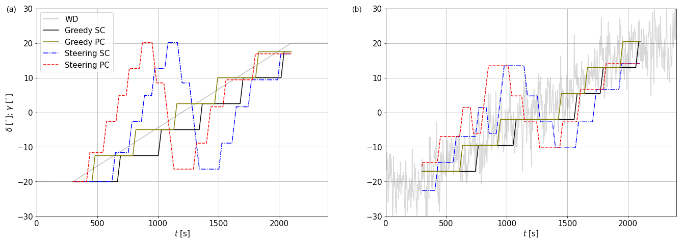
Figure 2 Examples of the engineering model's results for a wind direction change rate of $\mathit{\theta }=\mathrm{80}{}^{\circ }{\mathrm{h}}^{-\mathrm{1}}$. Gray lines indicate the wind direction of an (a) smooth and (b) turbulent time series. Black and yellow indicate greedy SC and PC; blue and red indicate wake steering SC and PC, respectively. A turbine spacing of 6 D is assumed, and $\stackrel{\mathrm{‾}}{\mathit{\delta }}=\mathrm{0}{}^{\circ }$ indicates the wind direction in which the turbine pair is aligned.

3.1.1 Example

Figure 2a illustrates an example displaying the wind direction signal (gray) and the orientation of the upstream turbine for four different yaw controllers. The smooth wind direction change experienced by the turbine is trailed by yaw actuator movement under traditional greedy SC (black). In its optimization, the engineering model tests for the preview time at which the highest power gain can be achieved; the corresponding result is shown in yellow. It is evident that the turbine yaws to the same new orientation but does so earlier, such that the wind direction reaches the orientation of the preview-controlled turbine right in between two consecutive actuator movements. This intuitively makes sense, as the optimum solution aims to limit misalignment. When adding turbulence (Fig. 2b), this is still true, although it is not as clearly visible. When applying the wake steering control (blue (SC) and red (PC) in Fig. 2a), a clear misalignment of the turbine with the wind direction can be observed. The misalignment increases as the wind direction approaches 0^∘ until it crosses over from a positive to a negative misalignment. When turbulence is introduced (Fig. 2b), the controllers become more conservative (smaller intentional misalignments), which is a direct consequence of the included uncertainty parameter, as discussed in Sect. 2.2.

3.2 Large-eddy simulations

This study uses revision 3475 of the PArallelized Large-eddy simulation Model (PALM, Maronga et al. (2020)). PALM uses a non-hydrostatic incompressible Boussinesq approximation of the Navier–Stokes equations. The exchange between the surface and the lowest grid cell in the vertical is handled following Monin–Obukhov similarity theory. Time integration is done by a third-order Runge–Kutta scheme, advection of momentum is performed by a fifth-order Wicker–Skamarock scheme, and subgrid-scale turbulence is modeled by applying Deardorff’s 1.5-order turbulence closure parameterization. The Coriolis parameter is computed for a latitude of 55^∘ N. The grid has a regular spacing of Δ= 5 m on a right-handed Cartesian coordinate system, but to save computational costs, the vertical grid size increases by 8 % per cell above the boundary layer height.

The simulation chain consists of three simulations: first, a precursor simulation to generate realistic inflow conditions; second, a simulation in which the wind direction in the domain is changed; and third, a main simulation that contains two turbines.

3.2.1 Precursor simulation

In the precursor simulation, a realistic turbulent flow is generated by adding random perturbations to an initially laminar flow. The chaotic behavior of the modeled boundary layer generates turbulent structures at a range of scales until a stationary state is reached after several hours of simulation time. This study only considers one atmospheric condition, a conventionally neutral boundary layer with a hub height (90 m) wind speed of 8.3 m s⁻¹. The hub height turbulence intensity in this boundary layer is 10.3 %, while the power law wind shear exponent and vertical wind veer between lower and upper tip height are 0.17 and 2.0^∘, respectively. Although the effect of atmospheric conditions (wind speed, stability) on the effectiveness of preview control is deemed interesting, investigating this was considered out of the scope of the current study. A short discussion is included in Sect. 5.2.

3.2.2 Simulation of wind direction changes

In this study, the wind direction is changed by applying the methodology developed by Stieren et al. (2021), in which the momentum equations are modified by adding an artificial Coriolis force F_θ:

$$\begin{array}{}\text{(6)}& F_{\mathit{\theta }}=-\mathit{\theta }\left(t\right)u_j{\mathit{ϵ}}_{ij\mathrm{3}},\end{array}$$

in which θ(t) is the forced wind direction change rate, u_j are the wind speed components, and ϵ is the Levi–Civita symbol. This is an engineering approach in which the centrifugal and Euler force are neglected. Although not physical, Stieren et al. (2021) demonstrated that the observed wind direction compares well with the forced signal. This methodology allows for changing the wind direction at a constant rate (θ(t)=θ₀) as well as more realistic wind direction changes as observed in the field.

The code employed in Stieren et al. (2021) used a concurrent precursor inflow method with a fringe region, ensuring undisturbed inflow in the cyclic boundary conditions that are required for the implementation of this method to change the wind direction. PALM does not have this feature implemented, so, for this reason, an intermediate simulation is carried out. An empty domain (no turbines) with cyclic horizontal boundary conditions is initialized with the turbulent flow generated by the precursor simulation. A predetermined θ(t) forces the wind direction to change in the whole model domain simultaneously, and a slice in the yz plane (crosswise and vertical dimensions) is saved to use as the inflow in the main run. This information comprises the three wind speed components as well as the potential temperature and the subgrid-scale kinetic energy.

3.2.3 Main simulation

In the main simulation, two NREL 5 MW turbines are simulated using an actuator disk model with rotation (ADMR) similar to Wu and Porté-Agel (2011) as described in Dörenkämper et al. (2015). The turbine pair has a spacing of 6 D and is aligned for a wind direction of $\mathit{\delta }=\mathrm{270}{}^{\circ }$. In a domain with non-cyclic boundary conditions in the streamwise direction, the yz plane saved from the simulation discussed in the previous section is used as the inflow 25 D upstream of the first turbine. As a result, a transient wind direction change propagates through the domain with a time-varying wind speed (fluctuations around the mean) and direction (fluctuations around the mean on top of the forced signal) rather than collectively in the whole domain, as was the case in Stieren et al. (2021). This is important for this study, as an incoming wind direction change needs to be detected before it reaches the turbines in order for PC to be beneficial. Additionally, a time delay between the upstream turbine and the downstream turbine experiencing a wind direction change is likely more realistic. Figure 3 displays examples of the flow field with the two turbines that illustrate a wind direction change propagating through the domain. Besides the wind direction change, large turbulent structures with different wind speeds can be observed. Additionally, the misalignment of the upstream turbine indicates the controller lag.

Since the boundary conditions in the streamwise direction are non-cyclic, the introduced wind direction change results in a gradient of the horizontal wind speed components in the streamwise direction ($\partial \stackrel{\mathrm{‾}}{u}/\partial x$). This needs to be compensated for in either the crosswise or vertical direction to obey the conservation of mass. Because of the cyclic boundary conditions in the crosswise direction, this gradient cannot be compensated for with $\partial \stackrel{\mathrm{‾}}{v}/\partial y$. Therefore, the gradient $\partial \stackrel{\mathrm{‾}}{u}/\partial x$ is compensated for by $\partial \stackrel{\mathrm{‾}}{w}/\partial z$, introducing a vertical velocity that alters the wind speed and direction profiles over time. Since all experiments with different controllers experienced the same effect, it is not considered detrimental to the outcome of this study.

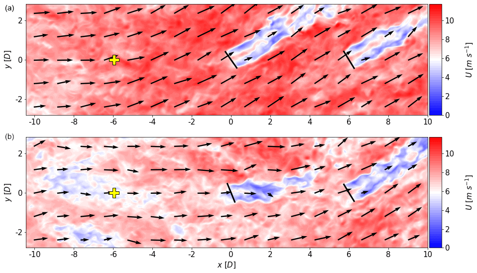
Figure 3 Examples of wind fields illustrating a wind direction change propagating through the domain. Wind field (b) is taken 140 s after wind field (a). The background color indicates the wind speed and the arrows indicate the wind direction. The solid black lines indicate the turbines, both of which are operating in greedy control without preview information. The yellow markers indicate the location of the virtual met mast.

Standard control. The input for SC consists of information at the position of two grid cells (10 m) upstream of the turbine. A point in front of the turbine was chosen to mimic a nacelle wind vane that is not disturbed by the rotor. This allows for a fairer comparison of the model results, as the preview control wind vane (see below) is not disturbed by any rotor.

Preview control. PC is implemented in the form of a virtual wind vane at hub height on a meteorological (met) mast. The virtual met mast is located at a fixed position upstream of the first turbine for $\mathit{\delta }=\mathrm{0}{}^{\circ }$, the wind direction in which the turbine pair are aligned. In Sect. 4.1, the optimum preview time is estimated with the engineering model before being converted to a preview distance considering a hub height wind speed of 8.3 m s⁻¹. The position of the vertical met mast is indicated in yellow in Fig. 3. Although the relative position of a measurement point upstream of the rotor changes with wind direction, a fixed position of the virtual vane is deemed sufficient, as wake steering is limited to $\left|\stackrel{\mathrm{‾}}{\mathit{\delta }}\right|<\mathrm{20}{}^{\circ }$ (Sect. 2.2). The wind direction signal is directly passed to the controller assuming Taylor's hypothesis of frozen turbulence, meaning that no wind evolution is considered, although it is deemed important, as pointed out in Laks et al. (2010). As the signal is subject to advection and heterogeneity, this method does not resemble a perfect forecast.

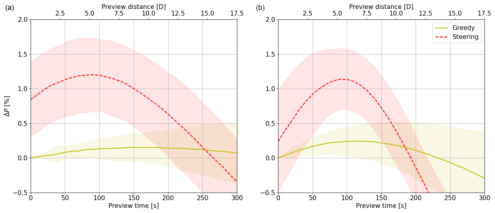
Figure 4 Turbine pair power gain ΔP of greedy control (yellow) and wake steering control (red) with PC relative to greedy SC as a function of preview time for wind direction change rates of $\mathit{\theta }=\mathrm{80}{}^{\circ }$ h⁻¹ (a) and $\mathit{\theta }=\mathrm{160}{}^{\circ }$ h⁻¹ (b). Lines indicate the mean and shaded areas indicate the 95 % confidence interval over 50 turbulent time series.

4 Results

4.1 Engineering model

4.1.1 Theoretical linear wind direction changes

In this section, a wind direction change of 40^∘ is simulated with different change rates θ using the engineering model. Starting from a constant $\mathit{\delta }=-\mathrm{20}$^∘ for the first 300 s (spin-up, not used for analysis), the direction changes linearly to $\mathit{\delta }=+\mathrm{20}$^∘, where it remains for the last 300 s (spin-down, not used for analysis). As described in Sect. 3.1, 50 different seeds of turbulent noise are added on top of this linear wind direction change to statistically analyze the impact of turbulence. Values for the wind speed (U_h=8.30 m s⁻¹), wind shear and veer over the rotor area (α=0.17, $\mathit{\delta }\mathit{\alpha }=\mathrm{2}{}^{\circ }$) and, consequently, the rotor equivalent wind speed ($U_{\mathrm{eq},\mathrm{up}}=\mathrm{8.25}$ m s⁻¹) are taken from LES (Sect. 3.2.1).

Figure 4 displays the turbine pair power gain of PC relative to SC as a function of preview time for two wind direction change rates: θ=80^∘ h⁻¹ (Fig. 4a) and θ=160^∘ h⁻¹ (Fig. 4b). First focusing on greedy control, the maximum power gain from PC is higher for a larger θ, whereas the optimal preview time is smaller. With a faster wind direction change, the misalignment of the SC turbine is larger, resulting in higher power losses. As a result, the benefit of PC is greater. When the turbine yaws too early it also loses power, explaining the decreasing gains for longer preview times and the shorter optimal preview time for a larger θ. Although an optimum is found, PC seems relatively insensitive to the preview time, as indicated by a relatively flat curve. Lastly, the uncertainty increases with larger preview times, as illustrated by the 95 % confidence interval.

Now, focusing on the wake steering controller, it can be seen that wake steering with SC (preview time = 0 s) is estimated to achieve a power gain of 0.8 % (for θ=80^∘ h⁻¹), whereas PC with optimum preview time results in a power gain of 1.2 %. This difference exceeds the power gain achieved by PC in the greedy control of 0.2 %, which suggests that wake steering can benefit more from PC than greedy control. This is strengthened by the findings from the θ=160^∘ h⁻¹ case, where wake steering with SC only achieves a power gain of 0.25 %, with the 95 % confidence interval also displaying power losses. PC with the optimum preview time gives a power gain of 1.3 %, again far exceeding the 0.3 % gain expected from greedy control.

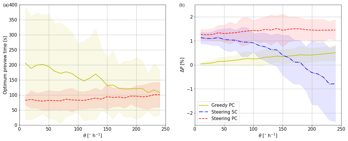
Figure 5 Optimal preview time (a) and corresponding power gain relative to greedy SC (b) as a function of θ. Yellow indicates greedy PC, blue indicates wake steering SC, and red indicates wake steering PC. Lines indicate the mean and shaded areas indicate the 95 % confidence interval over 50 turbulent time series.

Figure 5 represents the optimal preview time and corresponding power gain as a function of θ. Focusing first on the optimal preview time for greedy control in Fig. 5a, the mean over the turbulent simulations indicates decreasing optimal preview times for increasing θ, corresponding to the findings in Fig. 4. The uncertainty decreases with increasing θ, as dynamic changes become more dominant, preventing the yaw controller from chasing turbulence. As for wake steering, the optimal preview time seems to be relatively insensitive to θ, showing an almost constant value between 80 and 100 s. This value likely depends on the updating frequency of the yaw controller, but it is an interesting finding that would make the implementation of PC in the field easier.

The maximum achievable power gain with an optimal preview time (Fig. 5b) appears to increase linearly with θ for greedy control. The mean ranges from 0.1 % for slow wind direction changes to almost 0.8 % for extreme events, while the uncertainty slightly increases with θ. This is similar to PC in wake steering, which shows power gains ranging from 1.3 % to 1.7 %. Steering SC shows power gains very similar to PC for small θ, but for larger θ the gains rapidly decrease and turn into losses (erroneous steering). Especially under these fast-changing conditions, wake steering can benefit the most from PC, as it provides consistent power gains.

Figure 6 Histogram of optimum preview time (a) and corresponding power gain (b) when using wind direction measurements from a met mast. Lines indicate the median optimum preview time (a) and corresponding mean power gain (b). Colors correspond to those used in Fig. 5.

4.1.2 Wind direction time series from met mast measurements

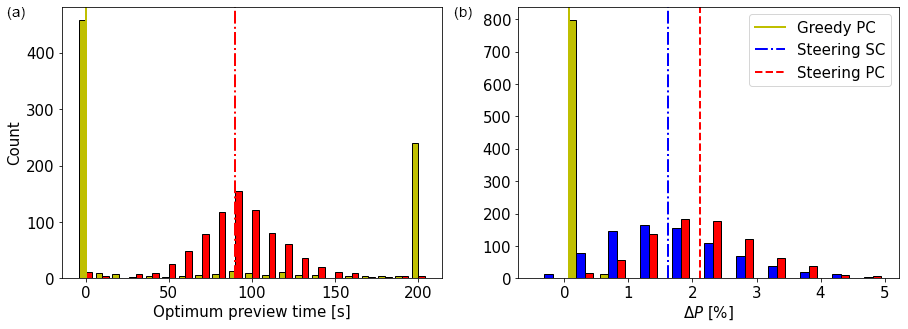
In addition to the linear wind direction changes considered in the previous section, more realistic wind direction changes are studied here using the engineering model. Wind vane and anemometer measurements at hub height (116 m) from an experimental campaign are used. This campaign was carried out between February and April 2021 at a slightly hilly onshore site in northeastern Germany located approximately 13.5 km from the Baltic Sea. For more details, the reader is referred to Sengers et al. (2023). The data are split into 1 h subsets, where again the first and last 300 s are disregarded as spin-up and spin-down times. Because this study limits its analysis to wind speeds around 8 m s⁻¹, only subsets with an average wind speed between 6 and 10 m s⁻¹ are considered, resulting in a total of 815 subsets. Other atmospheric characteristics (e.g., turbulence intensity, shear, stability) are not considered. For each subset, the average wind direction is assumed to coincide with the alignment of the turbine pair. The turbines are initialized with an orientation corresponding to the low-pass-filtered signal at the start of the hour. As preview times larger than 200 s do not seem to be relevant according to Fig. 5, the maximum preview time considered here is 200 s. Figure 6 displays the findings of this analysis in two histograms. The optimum preview time (Fig. 6a) for greedy control shows that the extreme values of 0 and 200 s often occur. These represent cases in which there was hardly any wind direction change within the hour. In these cases, either no yawing takes place and PC and SC estimate the same power, displayed here as a preview time of 0 s, or one yaw maneuver takes place, which is most beneficial when done as early as possible. Excluding these events, the results show a very flat distribution of optimal preview times. For wake steering, on the other hand, an approximately normal distribution with a median of 90 s is found, corresponding well to the results of Fig. 5.

The maximum power gain, displayed in (Fig. 6b), indicates that PC under greedy operation is not very beneficial. With a mean gain of 0.06 %, much lower power gains are expected from realistic wind direction data than from previous tests with a linear wind direction change. Wake steering with SC shows an approximately normal distribution of power gains with a mean of 1.62 %, whereas PC increases this to 2.12 %, again suggesting that PC is especially beneficial when applying wake steering.

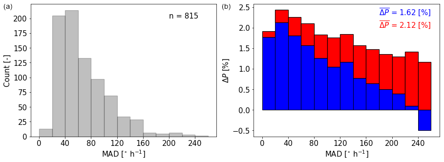
Figure 7 (a) Histogram of met mast data binned in mean of absolute differences (MAD). (b) Power gain of steering SC relative to greedy SC (blue) and power gain of steering PC relative to greedy SC (red). Power gains averaged over all 815 cases are noted in the top right corner.

To investigate under what conditions steering SC and PC are most beneficial, the power gains are studied as a function of the characteristics of the wind direction signal. For this, the mean of absolute differences (MAD) is calculated as

$$\begin{array}{}\text{(7)}& \mathrm{MAD}={\displaystyle \frac{\mathrm{1}}{T}}\sum _{t=\mathrm{2}}^T|{\mathit{\delta }}_{\mathrm{lp},t}-{\mathit{\delta }}_{\mathrm{lp},t-\mathrm{1}}|,\end{array}$$

which computes the mean of the absolute differences in wind directions of consecutive time steps. Here, δ_lp is again the low-pass-filtered time series obtained using a cutoff frequency of 0.0037 Hz. Because the signal is already low-pass filtered, MAD does not relate to the small-scale turbulence, but rather to larger-scale wind direction fluctuations. The unit of MAD ^∘ s⁻¹, which, for interpretability, is converted to ^∘ s⁻¹. The histogram in Fig. 7a displays that the majority of the cases represent steady conditions with only a wind direction change. However, several cases with large dynamic changes are observed. Figure 7b shows in blue the average power gain of steering SC compared to greedy SC as a function of MAD. The largest gains are found for small wind direction changes, as this approaches a steady state for which the controller was developed. However, power losses are found for large values of MAD. Despite their rare occurrence, these cases undermine confidence in the wake steering strategy. It is especially under these conditions that PC has a large added benefit. Steering PC shows a more consistent power gain relative to greedy SC (red) regardless of the characteristics of the wind direction time series; hence, a power gain using wake steering seems guaranteed. The difference between the blue and red bars illustrates that when the signal is relatively steady, PC only has a small benefit. However, the more the signal fluctuates (increasing MAD), the larger the benefit of PC, as the yaw controller is now able to anticipate incoming wind direction changes.

4.2 Large-eddy simulations

In this section, LES results are used to validate the findings of the previous section and, with that, demonstrate the benefit of preview control. For this purpose, wind direction time series observed in the field are reproduced in LES. First, two examples are simulated (Sects. 4.2.1 and 4.2.2), one with a low and one with a high large-scale wind direction variability. Second, to approach statistical significance, multiple cases with similar characteristics are simulated. As LES is too expensive to use to obtain fully statistically significant results, only six seeds are performed, following the standard used in fatigue load estimation studies. To investigate the sensitivity of the preview controller performance, changes in both low-frequency (Sect. 4.2.3) and high-frequency fluctuations (Sect. 4.2.4) are considered to better understand the performance of the preview controller.

4.2.1 Case selection

Figure 8 illustrates the two simulated examples, in which the obtained wind direction signal at the upstream turbine is indicated in gray (raw) and black (low-pass filtered) and the forced signal (Sect. 3.2.2) in red. This forced signal is the low-pass-filtered wind direction measured at the met mast using the same cutoff frequency of 0.0037 Hz. It should be noted that besides the mean wind speed, no other meteorological conditions (e.g., shear, veer, stability) are evaluated on how well they match the simulated boundary layer characteristics.

Comparing the signals reveals that the main characteristics of the forced signal are reproduced. Differences are due to advection, as the wind direction signal is forced at the domain inflow boundary 25 D upstream of the turbine. Case 1 (Fig. 8a) represents a scenario in which wake steering with standard control is expected to obtain a large power gain. This case is considered to demonstrate that preview control is not detrimental to the power gain achieved with wake steering SC. Case 2 (Fig. 8b) illustrates an event in which wake steering with standard control is expected to see a power loss due to rapidly changing conditions, a scenario in which wake steering is expected to benefit greatly from preview control. A third case, which is of interest but may be less common, is provided in Appendix A. It represents a situation with strong fluctuations around $\mathit{\delta }=\mathrm{0}{}^{\circ }$.

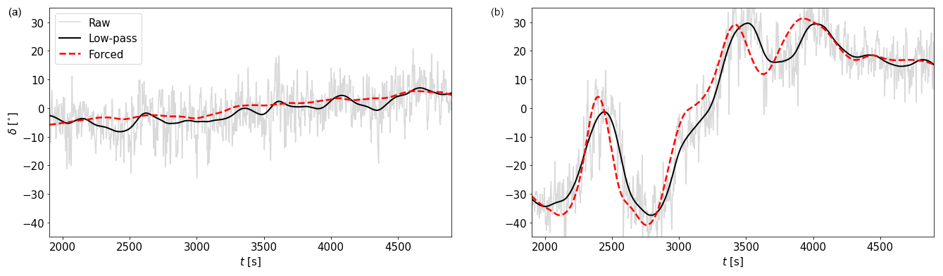
Figure 8 Simulated wind direction cases. Raw (gray) and low-pass-filtered (black) signals at the upstream turbine are shown, as well as the forced (dashed red) signal. (a) Case 1: a slowly varying wind direction change. (b) Case 2: a fast-varying wind direction change.

The first 600 s of the simulation are used to move from δ= 0^∘ to the initial δ, the start of the low-pass-filtered time series. At 600 s, both turbines are turned on and are given an additional 600 s to spin up while the mean wind direction remains constant. Corresponding to Sect. 4.1, the first 300 s of the field time series are omitted. After 1500 s, the wind direction signal used for analysis enters the domain, but it takes 400 s for this information to flow from the inflow boundary to the upstream turbine. Altogether, the first 1900 s of the simulation are omitted, whereas the following 3000 s are used for analysis. Corresponding to the findings in Sect. 4.1.2, the preview time was chosen as 90 s, equivalent to a preview distance of 750 m or 6 D for an average hub height wind speed of 8.3 m s⁻¹.

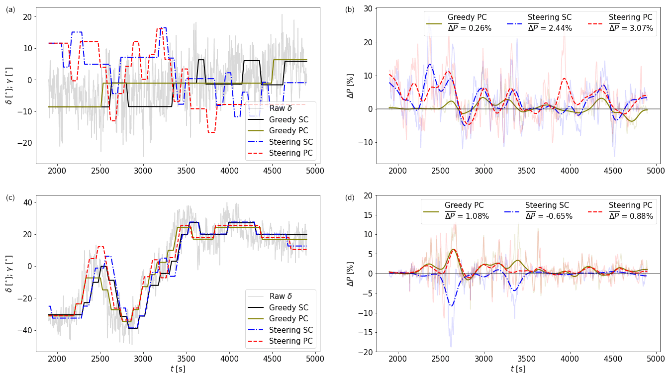
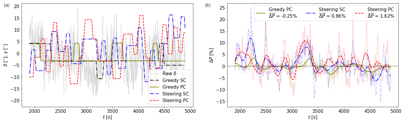
Figure 9 LES results for Case 1 (a–b) and Case 2 (c–d). The left column shows the wind direction δ (gray, see Fig. 8) and orientations of the upstream turbine γ (colors). The right column shows the raw (transparent) and low-pass-filtered (opaque) power gain ΔP relative to greedy SC. The gain averaged over the simulation $\stackrel{\mathrm{‾}}{\mathrm{\Delta }P}$ is indicated in the legend.

4.2.2 Performance of the controllers for selected cases

Figure 9 shows the wind direction (δ) and yaw angle (ϕ) of the upstream turbine (left column) and the corresponding power gain relative to greedy SC (right column). Since the raw power gain signal (transparent) is rather noisy, the low-pass-filtered (also using a cutoff frequency of 0.0037 Hz) signal is also included and is shown by opaque lines. In Case 1 (Fig. 9a–b), the turbine orientation of greedy SC illustrates that small-scale turbulence has a large influence on the controller actions, as is evident from the maneuvers in the direction opposing the large-scale wind direction change (e.g., at 2800 s). Enabling PC eliminates this behavior, although this is likely a coincidence rather than an effect of PC. A textbook-like situation can be seen at around 2500 s, where the PC turbine yaws earlier than the SC turbine, resulting in a small power gain due to a better orientation. This is directly followed by a power loss, as the wake reaching the downstream turbine is slightly stronger. Averaged over the whole simulation, greedy PC achieves a small power gain of $\stackrel{\mathrm{‾}}{\mathrm{\Delta }P}=$ 0.26 %. Wake steering results in more yaw maneuvers than greedy control. For the first half of the simulation, the misalignment is characterized by positive angles, whereas the second half is characterized by negative angles. The orientation of the SC and PC turbines deviates from a temporally shifted signal due to the heterogeneity between the two locations from which information is acquired. Wake steering with SC results in $\stackrel{\mathrm{‾}}{\mathrm{\Delta }P}=$ 2.44 %, which is increased to $\stackrel{\mathrm{‾}}{\mathrm{\Delta }P}=$ 3.07 % when PC is enabled. This suggests that PC is not detrimental to the power gain achieved with steering SC and can increase this gain even further.

In Case 2 (Fig. 9c–d), wake steering with SC results in a power loss of $\stackrel{\mathrm{‾}}{\mathrm{\Delta }P}=-\mathrm{0.65}$ %. This is mainly due to two events that produce a significant power loss for several minutes. Both events are characterized by the upstream turbine yawing to a certain orientation exactly when the wind direction quickly rotates in the other direction, resulting in a large misalignment and a corresponding power loss. Enabling PC converts this power loss into a gain of $\stackrel{\mathrm{‾}}{\mathrm{\Delta }P}=$ 0.88 %, mainly achieved by eliminating these events. This suggests that PC could be used to avoid erroneous steering. It is noteworthy that in this case, greedy PC actually achieves the largest power gain ($\stackrel{\mathrm{‾}}{\mathrm{\Delta }P}=$ 1.08 %). This is partially due to the wind direction being only in the region where wake steering is deemed useful ($\left|\mathit{\delta }\right|<\mathrm{20}{}^{\circ }$) during a small part of the simulation.

4.2.3 Variation of low-frequency fluctuations

As mentioned before, an analysis with six seeds is performed to approach statistical significance. In this section, the variation of low-frequency fluctuations is considered.

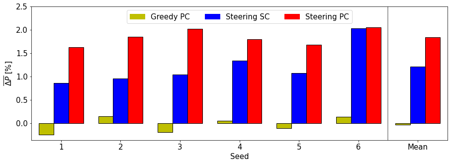
Besides Case 1 from the previous section, five more cases are randomly selected from all met mast data with a low variability (MAD < 40^∘ h⁻¹, Fig. 7). Figure 10a displays these results; the six seeds are displayed (Seed 1 indicates Case 1), as are their means on the far right. The benefit of PC in greedy operation is negligible, as the power gains of the upstream turbine due to a better alignment do not outweigh the power losses observed for the downstream turbine due to a stronger wake. It is, however, expected that greedy PC outperforms greedy SC in scenarios where the downstream turbine is not heavily waked. Steering SC achieves a power gain of 1.24 % on average, which is increased to 1.85 % when PC is enabled. The differences between the seeds are substantial, which can be directly linked to the characteristics of the wind direction signal. For instance, in Seeds 1 and 6, a partial wake situation occurs for a substantial part of the simulation. However, the other simulations display a full wake situation for almost the whole simulation, resulting in lower power gains. The effectiveness of PC can also be directly linked to the nature of the wind direction signal, as a very steady, non-changing wind direction will not benefit from PC. Lastly, these results are subject to small-scale turbulence, as pointed out in Sect. 4.1, as well as the controller design. It is therefore deemed important to look at the statistics (here, the mean), rather than the individual seeds.

Due to a lower occurrence of cases with a very high variability corresponding to Case 2, five randomly drawn cases with a MAD > 140^∘ h⁻¹ make up the remaining seeds. Note that the variability between these seeds is larger than between the six low-variability seeds discussed in Fig. 10a. It can be seen that Case 2, indicated as Seed 1 in Fig. 10b, was actually the only time series that resulted in a power loss for steering SC. On average, the power gain achieved with steering SC is still relatively small ($\stackrel{\mathrm{‾}}{\mathrm{\Delta }P}=$ 0.44 %). PC is able to increase this gain to 1.32 %, which is a larger benefit than observed for the low-variability seeds. Also, greedy control benefits more from PC in cases with a high variability. Large differences between the seeds can be observed, the most striking being the slight power loss observed for steering PC relative to steering SC in Seed 6. Like before, this is attributed to the chaotic nature of the simulations and is expected to be subject to small-scale turbulence and controller design. Nevertheless, these results are believed to make a convincing case for the use of preview wind direction information, especially in wake steering operation.

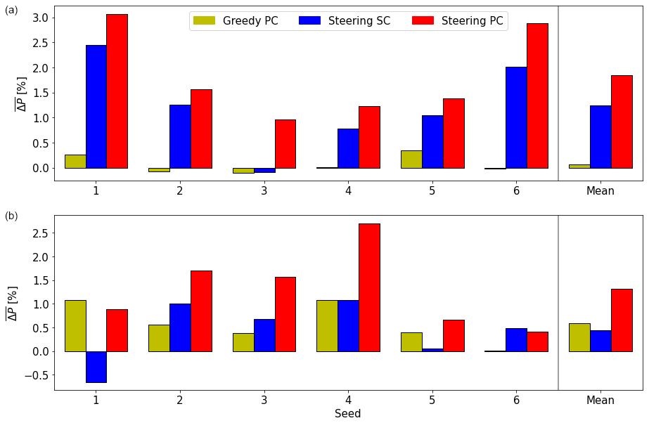
Figure 10 Seed analysis of low-frequency fluctuations. Averaged power gains $\stackrel{\mathrm{‾}}{\mathrm{\Delta }P}$ of six seeds for slowly varying MAD < 40^∘ h⁻¹ (a) and fast-varying MAD > 140^∘ h⁻¹ (b) wind direction changes. The average of all seeds is indicated on the far right.

Figure 11 Same as Fig. 10, but for the seed analysis of high-frequency fluctuations.

4.2.4 Variation of high-frequency fluctuations

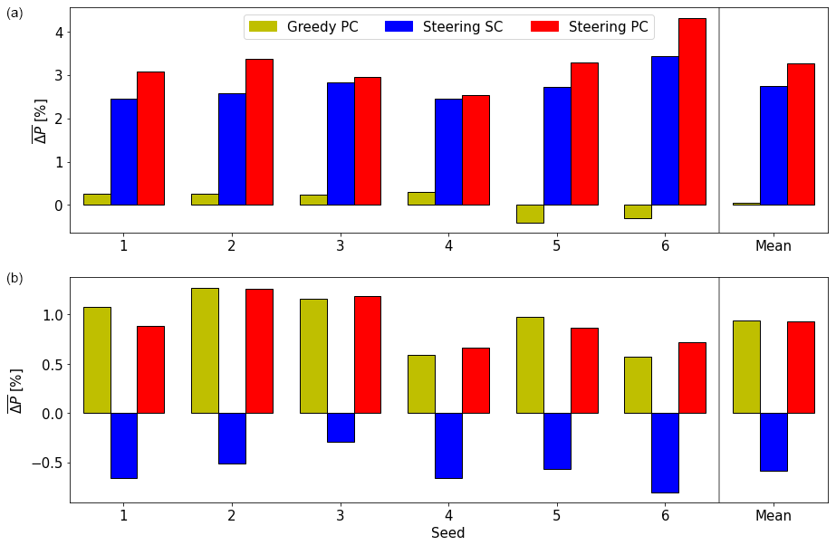
As already illustrated in Sect. 4.1, high-frequency turbulence has a significant effect on the power yield and therefore on the benefit of PC. In addition to the seed analysis performed in Sect. 4.2.3 by varying the low-frequency characteristics of the wind direction signal, a similar analysis is performed by varying the high-frequency characteristics. Focusing again on Cases 1 and 2, the simulations are forced by the same low-frequency signal, but both turbines are shifted laterally in the domain in increments of 2.5 D to induce a different high-frequency wind direction component.

Figure 11a displays that for Case 1, greedy PC results in a small power gain in four out of six seeds but losses in the remaining two, resulting in a very small gain when averaged over all seeds. Steering SC shows $\stackrel{\mathrm{‾}}{\mathrm{\Delta }P}>\mathrm{2}\mathit{\%}$ for all seeds, averaging a gain of 2.74 %. With PC enabled, this increases to 3.26 %, with a substantial spread between the seeds. For instance, PC's benefit in Seed 4 is negligible, but PC adds almost a full percentage point of power gain in Seed 6.

Figure 11b shows the same analysis for Case 2. Steering SC results in a power loss in all seeds, with a mean power loss of $\stackrel{\mathrm{‾}}{\mathrm{\Delta }P}=-\mathrm{0.58}\mathit{\%}$. This loss is converted into a gain of 0.93 % when PC is enabled, clearly demonstrating that PC is able to prevent erroneous yawing. Greedy PC achieves the highest gain, $\stackrel{\mathrm{‾}}{\mathrm{\Delta }P}=$ 0.94 %, corresponding to the results discussed in Sect. 4.2.2.

The results from all cases and seeds sketch the clear picture that wake steering benefits substantially from preview control. Since the differences between seeds in Fig. 10 are larger than those in Fig. 11, it is concluded that the magnitude of this benefit mainly depends on the low-frequency wind direction variability (Sect. 4.2.3). The high-frequency variability (turbulence) plays a secondary role, as these fluctuations have a smaller effect on the moving average of wind direction used by the yaw controller to decide when to initiate a yaw maneuver.

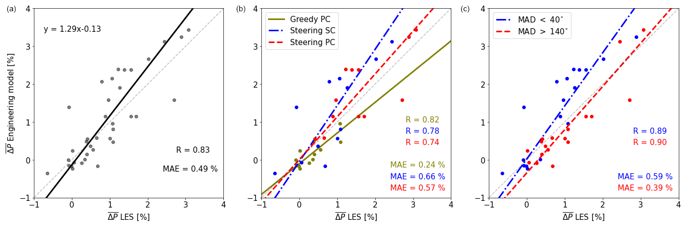
Figure 12 Comparison of the engineering model and LES in estimating the power gain $\stackrel{\mathrm{‾}}{\mathrm{\Delta }P}$. The Pearson correlation coefficient (R), mean absolute error (MAE) and orthogonal distance regression fit are indicated. (a) All results, (b) the results split by control strategy and (c) the results split by variability of the wind direction signal.

4.3 Comparison of large-eddy simulation and engineering model results

In this section, the power gains computed with the engineering model are compared to those obtained with LES. While acknowledging that models are inherently imperfect, the LES results are considered the truth here. The wind direction signal at the turbine of the greedy SC LES run is passed to the engineering model. It should be noted that in LES, the time series of wind directions at the turbine differ slightly between the simulations since the turbines do not exert the same thrust force on the incoming flow due to their different orientations. The analysis is restricted to the 12 low-frequency varying simulations discussed in Sect. 4.2.3.

Figure 12a shows that the engineering model has a mean absolute error MAE = 0.49 % and a correlation coefficient R=0.83. The fitted linear relation indicates that large gains are typically overestimated with the engineering model. Splitting the data by control strategy (Fig. 12b) reveals that this systematic bias is mainly caused by steering SC. Lastly, splitting the data into low (MAD < 40^∘) and high (MAD > 140^∘) variability in Fig. 12c illustrates that the engineering model struggles in the low-variability cases. This is likely due to the relatively long period of the full wake situation, which emphasizes any inaccuracies of the wake model.

Considering the assumptions made in the engineering model (e.g., a constant wind speed) and the difference in computational costs (≈ 1500 CPU hours for LES and ≈ 0.1 CPU hours for the engineering model), the accuracy of the engineering model is considered acceptable. This gives some credibility to the results discussed in Sect. 4.1. The next steps to improve the engineering model could be to include the time-varying wind speed and veer, which are currently assumed to be constant. This would likely result in an increased accuracy at the cost of slowing down the model. Additionally, as the engineering model is subject to the underlying DART wake model, improvements there will likely also result in a more accurate engineering model.

5 Discussion

The results presented in this study demonstrate the benefit of preview wind direction control. However, the authors are aware that many assumptions were made to show this proof of concept. These, as well as their implications for future work, are described in this section.

5.1 Comparison to existing literature

The body of existing literature on the topic of preview wind direction control for wake steering purposes is small. However, some interesting points can be noted when comparing the current results to those in Simley et al. (2021b). Both studies use an engineering model with a similar controller logic and consider wind speed. Interestingly, an identical optimal preview time of 90 s was identified in both works.

Using this optimum preview time and assuming perfect preview measurements, Simley et al. (2021b) reported a power gain ranging from 5.8 % for wake steering with standard control to 8.9 % when preview control was enabled, representing an increase of 55 %. Performing a similar exercise, the current study found an increase of 31 %: from 1.62 % for standard to 2.12 % for preview wake steering control. These differences are subject to the different engineering models used, the size of the data set, the turbine spacing, and assumptions about the average wind direction. Regardless, both studies show a significant increase in power gain when using perfect preview information.

Lastly, Simley et al. (2021b) did not find any benefit of preview control in wake steering operation when feeding realistic wind direction information to the engineering model. By contrast, in the even more realistic environment of large-eddy simulations, this study demonstrated a significant power gain when using imperfect preview information. It should be noted that measurement errors due to device imperfections are not considered here. Regardless, this is an important result that demonstrates that the concept of wake steering using preview wind direction information is worth pursuing in future work.

5.2 Generalizability

This study was restricted to studying a very limited range of conditions. Only one wind speed in the partial load range was considered, as well as only a single stratification and turbine layout. For this reason, the results presented in this work cannot be directly generalized.

Since the wake steering effectiveness is influenced by the atmospheric stratification (Vollmer et al., 2016; Simley et al., 2022), it is reasonable to assume that the benefit of preview control is also subject to stability. With similar reasoning, the wind speed is also expected to impact the benefit of preview control, as it was demonstrated to affect the effectiveness of wake steering (Simley et al., 2021a). Furthermore, the preview distance is directly subject to the wind speed, and fluctuations will add another layer of complexity in the forecasting of the incoming wind direction changes.

Besides atmospheric conditions, the benefit of preview control is likely also subject to the yaw controller logic. The controller logic not only affects the timing to initiate a yaw maneuver but could also have implications for the optimum preview time identified in this work.

A logical next step for future work would therefore be to assess the effectiveness of the preview control strategy for a wider range of atmospheric conditions, as well as its dependence on yaw controller logic. Additionally, simulations containing full wind farms with different layouts should be carried out to see how the benefit of preview control changes with scale. This increases the complexity of the problem, as it is for instance unclear where the preview information for downstream turbines should be obtained. This is further discussed in Sect. 5.4.

5.3 Large-eddy simulation considerations

As mentioned in Sect. 3.2.3, the use of non-cyclic boundary conditions introduces a vertical gradient $\partial w/\partial z$, which alters the wind speed and direction profiles over time. Although this is not considered to affect the outcome of this study as all controllers experience the same effect, it is deemed important for future work to quantify the effect of this behavior and possibly use a different simulation setup to prevent it.

More generally, it should be noted that in LES, the wind direction changes always propagate through the domain, allowing an incoming change to be detected at the preview measurement location before it reaches the turbine. In reality, there may be scenarios when changes occur at the preview measurement and turbine locations at the same time. This would reduce the benefit of preview wind direction control.

5.4 Forecasting wind direction changes

Arguably the most important task is creating a feasible method to forecast the incoming wind direction. This study assumes the presence of a wind vane on a met mast 6 D upstream of the first turbine, corresponding to an optimal preview time of 90 s for a wind speed of 8.3 m s⁻¹. Not only is it unfeasible to erect met masts upstream of each turbine pair, but it is also impossible to adapt the met mast location to varying wind speeds and directions. More feasible would be to use SCADA data from surrounding turbines, as explored in Rott et al. (2020). A disadvantage of this is that it would only provide information further downstream in the wind farm and not for the first row of turbines, which may be the most crucial for wake steering. Alternatively, the use of long-range lidars should be explored. It is difficult to obtain accurate wind direction estimates with lidars, as they only measure a line-of-sight velocity (LOS). The measured LOS can be affected by both wind speed and direction changes, as illustrated in Held and Mann (2019) for a two-beam lidar. When operating the lidar with plan position indicator (PPI) scans, a sinusoid can possibly be fitted to the LOS measurements, as done in Theuer et al. (2020). This would, however, result in a relatively low update frequency and spatial averaging over a large area. Alternatively, multiple (at least two) lidars targeting the same points upstream can be installed at opposite sides of the wind farm; these can be used to reconstruct two wind speed components and consequently the wind direction (van Dooren et al., 2016). Lastly, lidar-based and SCADA-based forecasts can be combined, as done for wind speed in Theuer et al. (2022).

Regardless of what forecasting method is used, the smoothing of raw signals can be done with wind field estimation approaches using surrogate models (e.g., Doekemeijer et al., 2018; Sinner et al., 2020). The forecasting method's measurement error should be quantified, and how this error affects the effectiveness of preview control should be investigated. As the preview quality of these new methods is likely lower than that of a virtual met mast, power gains from preview control could be lower than illustrated in this work. However, given the substantiality of the gains demonstrated here, preview control using lower-quality wind direction signals still has the potential to provide significant power gains.

5.5 Yaw controller

In this study, a very simple controller was used that bases its yawing decisions on whether the turbine misalignment exceeds a preset limit of 7.5^∘, after which it blindly yaws to its next orientation. As discussed in Sect. 5.2, the yaw controller logic is expected to affect the effectiveness of preview control. Aggressive controllers are better able to follow wind direction changes, resulting in higher power production at the cost of more yaw maneuvers; therefore, the added value of preview control might be small. Likewise, conservative controllers likely benefit more (i.e., have a higher power gain compared to SC) from the use of preview information.

However, upon utilizing preview information, more intelligent controllers could be developed that, for instance, schedule the next maneuver. This could be used to mitigate frequent yawing, especially switching from positive to negative misalignments and vice versa, as seen in the extra case shown in Appendix A. A strong candidate is model predictive control (e.g., Spencer et al., 2011), which has been well researched for wind turbine blade pitch and generator torque control but has only recently been considered for yaw control. For instance, Song et al. (2019) formulated a model predictive controller that uses wind direction preview and realistic yaw dynamics for the greedy control of a single wind turbine. Model predictive control for wake steering remains a topic to be explored in future research.

5.6 Effect of preview control on yawing action and loads

As can be seen in Figs. 2 and 9, the number of yaw maneuvers in wake steering is much higher than in greedy control, which is well described in the literature (e.g., Bossanyi, 2019; Kanev, 2020). However, preview control does not seem to affect the number of yaw maneuvers, at least not as long as the same yaw controller is used.

A detailed analysis of how preview control affects turbine loads was considered out of the scope of the current work. The effect of wake steering on loads is complicated and heavily discussed in the literature (Houck, 2021, and references therein). It can be hypothesized that preview control reduces the loads on the upstream turbine since extreme misalignments are avoided (e.g., Fig. 9c). Since the wake will be more successfully steered away from the downstream turbine, the loads on this turbine are also expected to be lower.

6 Conclusions

This study has explored the use of preview wind direction information for wake steering control. An engineering model based on the Data-driven wAke steeRing surrogaTe model (DART) used wind direction time series to estimate power yields with perfect preview information. For this purpose, a turbine pair with a spacing of six rotor diameters was considered in a turbulent flow with a constant wind speed in the partial load range. Based on theoretical linear wind direction changes and later on field measurement data, the results of the engineering model identify an optimum preview time of 90 s for the considered controller, atmospheric conditions, and farm characteristics. Preview control results in an overall power gain, with the highest benefit obtained when the wind direction changes rapidly.

These results were validated by employing a large-eddy simulation model. Wind direction changes were forced in a neutral boundary layer containing the turbine pair. Preview information was taken from a virtual wind vane six rotor diameters upstream of the first turbine, corresponding to the previously determined optimum preview time of 90 s. A six-seed analysis of 3000 s simulations demonstrated that under large, low-frequency wind direction changes, wake steering with standard control results in only small power gains of 0.44 % on average and, occasionally, a power loss due to erroneous steering. In contrast, preview control achieves higher power gains of 1.32 % on average. In a second six-seed analysis with small low-frequency wind direction changes, wake steering with standard control achieved an average power gain of 1.24 %, which further increased to 1.85 % when enabling preview control. Fluctuations in the low-frequency region were shown to have a dominant effect on the performance of wake steering, particularly the effectiveness of preview control. High-frequency fluctuations (turbulence) are less important, as their impact on the yaw controller decision is smaller. Contrary to Simley et al. (2021b), who found no benefit of preview control with realistic wind direction information in wake steering operation, this study has demonstrated a significant power gain using realistic large-eddy simulation results.

This study has introduced many new research questions, such as how to feasibly obtain preview information, how the quality of these forecasts affects the effectiveness, and how to use this information in more intelligent controllers. However, the results demonstrate that wake steering can benefit considerably from preview wind direction control, making it a topic worth pursuing in future work.

Appendix A: Case with strong fluctuations around δ= 0^∘

Large-eddy simulation (LES) runs forced by an additional wind direction signal were performed, but these results were excluded from the main text for brevity. However, the results of this case might be of interest to some readers and have therefore been included in this appendix. The case represents a situation where δ= 0^∘ is crossed several times. The sign of the intentional misalignment switches several times, resulting in many and large yaw maneuvers, as can be seen in Fig. A1a. Although this case is typically viewed as detrimental for wake steering, here, steering standard control (SC) still obtains a power gain of $\stackrel{\mathrm{‾}}{\mathrm{\Delta }P}=$ 0.86 % (Fig. A1b), which is almost doubled when enabling preview control (PC). Greedy PC actually results in a power loss (a negative $\stackrel{\mathrm{‾}}{\mathrm{\Delta }P}$), which is likely due to a stronger wake reaching the downstream turbine as a consequence of a better alignment of the upstream turbine. Figure A2 shows the six-seed analysis with varying high-frequency fluctuations (see Sect. 4.2.4). Greedy PC has, on average, a very small power loss. Steering SC shows consistent power gains, averaging to $\stackrel{\mathrm{‾}}{\mathrm{\Delta }P}=$ 1.21 %, which is increased to 1.83 % when PC is enabled. Moreover, five out of six seeds show a substantial power gain for PC over SC. These results indicate that wake steering also benefits from preview wind direction control in this scenario.

Figure A1 Same as Fig. 9, but for a case where δ= 0^∘ is crossed several times.

Figure A2 Same as Fig. 11, but for a case where δ= 0^∘ is crossed several times.