Wake characteristics of a balloon wind turbine and aerodynamic analysis of its balloon using a large eddy simulation and actuator disk model

In the realm of novel technologies for generating electricity from renewable resources, an emerging category of wind energy converters called airborne wind energy systems (AWESs) has gained prominence. These pioneering systems employ tethered wings or aircraft that operate at higher atmospheric layers, enabling them to harness wind speeds surpassing conventional wind turbines' capabilities. The balloon wind turbine is one type of AWESs that utilizes the buoyancy effect to elevate the turbine to altitudes typically ranging from 400 to 1000 m. In this paper, the wake characteristics and aerodynamics of a balloon wind turbine were numerically investigated for different wind scenarios. Large eddy simulation, along with the actuator disk model, was employed to predict the wake behavior of the turbine. To improve the accuracy of the simulation results, a structured grid was generated and refined by using an algorithm to resolve about 80 % of the local turbulent kinetic energy in the wake. Results contributed to designing an optimized layout of wind farms and stability analysis of such systems. The capabilities of the hybrid large eddy simulation and actuator disk model (LES–ADM) when using the mesh generation algorithm were evaluated against the experimental data on a smaller wind turbine. The assessment revealed a good agreement between numerical and experimental results. While a weakened rotor wake was observed at the distance of 22.5 diameters downstream of the balloon turbine, the balloon wake disappeared at about 0.6 of that distance in all the wind scenarios. Vortices generated by the rotor and balloon started to merge at the tilt angle of 10^∘, which intensified the turbulence intensity at 10 diameters downstream of the turbine for the wind speeds of 7 and 10 m s⁻¹. By increasing the tilt angle, the lift force on the wings experienced a sharper increase with respect to that of the whole balloon, which signified a controlling system requirement for balancing such an extra lift force.

1 Introduction

The global development of wind farms has decreased the area of potential land for building new wind power plants. Meanwhile, wind streams near the ground are not permanent or stable due to surface roughness and obstacles. To overcome these limitations, airborne wind energy (AWE) technology has been proposed as a way to harvest wind power at higher altitudes (Paulig et al., 2013; Terink et al., 2011; Williams et al., 2007; Ruiterkamp and Sieberling, 2013; Günes et al., 2019; Cherubini et al., 2015). Compared to the conventional wind turbines at the 80 m altitude, estimations have revealed that wind power density will be 2–9 times higher at the altitude of 400–1000 m, respectively (Ahrens et al., 2013). Taking this into account, it is possible to benefit from relatively stable and continuous wind. Moreover, there is no need to occupy vast land areas and install towers for mounting wind turbines (Archer and Caldeira, 2009).

Figure 1 (a) Control volume and (b) annular element.

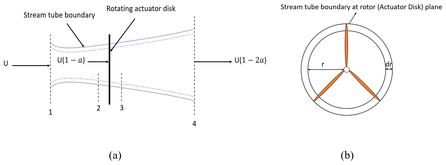
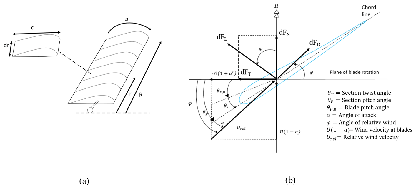
Figure 2 (a) Schematic of blade elements; dr, radial length of element; r, radius, (b) airfoil geometry for analysis of forces on a horizontal axis wind turbine.

According to Marvel et al. (2013), the maximum kinetic power that could be harvested from wind streams near the Earth's surface (extracted from conventional wind turbines) was estimated at 400 TW, while it is 1800 TW at 200–1000 m altitudes in the entire Earth. Many mechanical systems have so far been introduced in line with the development of airborne technology (Paulig et al., 2013; Terink et al., 2011; Williams et al., 2007; Ruiterkamp and Sieberling, 2013; Günes et al., 2019; Cherubini et al., 2015). For example, high-altitude kites (Paulig et al., 2013; Terink et al., 2011; Williams et al., 2007), gliders (Ruiterkamp and Sieberling, 2013; Sieberling, 2013), and Magnus effect turbines (Günes et al., 2019) are various types of airborne wind energy systems. Among these, the balloon wind turbine, also known as the buoyant airborne turbine (Altaeros, 2022), has relatively simpler take-off and landing maneuvers due to the buoyancy effect, which makes it suitable for deployment in various locations and temporary power generation where rapid setup is required. Moreover, these machines have minimal visual impact and can operate at higher altitudes, 400–1000 m, where wind speeds tend to be stronger and more consistent, which allows them to harness more energy compared to other AWE systems operating at lower altitudes. However, these turbines may have limitations in terms of scalability for large-scale energy generation projects. Also, employing these turbines requires adherence to aviation regulations and safety standards. And servicing and repairing components at high altitudes or remote locations may involve additional logistical complexities and costs which can be complex. To mitigate these limitations, balloon wind turbines can be installed closely together within a rectangular layout. The proximity of turbines allows for satisfying higher power output requirements and efficient use of the available airspace, and it enables easier maintenance and control of the turbines. In wind farms for these turbines, the wake of one turbine can affect the performance and efficiency of neighboring turbines. A high-fidelity study allows for a detailed analysis of wake interactions, including the velocity deficits, turbulence, and impact on power generation, which can help optimize the layout and spacing of the turbines.

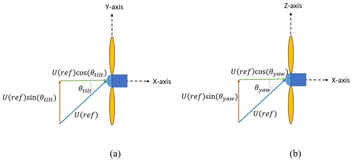
Figure 3 (a) The 3D model of the balloon with a duct (NACA 9415 airfoil cross-section) and four wings (n0009sm-il airfoil cross-section) and (b) geomatic dimensions of the balloon and AD position inside it. Yaw (θ_yaw) and tilt (θ_tilt) angles represent the angle between the rotor axis and its horizontal and vertical axes, respectively (Fig. 4). Since the balloon and rotor are symmetric with respect to x–y and x–z planes (Fig. 3), yawed and tilted configurations are technically equivalent. Therefore, only the effects of tilt angle on the wake flow were considered in this numerical investigation.

Figure 4 (a) Tilt configuration and (b) yaw configuration.

The balloon of these turbines acts like a restricting duct that can raise wind speed, thereby increasing the rate of energy extraction from the wind (Bontempo and Manna, 2016; Van Bussel, 2007; Hansen et al., 2000; Lewis et al., 1977). Accordingly, Inglis (1979) corrected the power limitation of wind turbines obtained by the Betz theory (Betz, 1926) by considering the wake rotation and the mixture of the wake with the free stream. Rauh and Seelert (1984) claimed that the output power obtained in the Betz theory did not lead to accurate results. Accordingly, when calculating this power by the Betz theory, the pressure at the inlet and outlet of the control volume was assumed to be the same, while such an assumption was inconsistent with the pressure drop at the turbine location. Considering the pressure variations in this control volume, a modified equation for calculating the power was introduced.

Several studies have been conducted on ducted wind turbines (DWTs) (Ahmadi Asl et al., 2017; Bontempo and Manna, 2016; Dighe et al., 2020; Lin and Porté-Agel, 2019; Tang et al., 2018; Lewis et al., 1977; Hansen et al., 2000; Van Bussel, 2007). Among them, experimental and theoretical studies by Lewis et al. (1977) exhibited an increase in DWT's power by a coefficient compared to bare turbines. They proved this coefficient equaled the total thrust of the duct and turbine to the turbine thrust alone. Van Bussel (2007) presented the improved momentum theory to investigate the effects of the duct on rotor performance. The mass flow rate of the air passing the duct was found to be directly related to the ratio of the duct's outlet area to its throat area.

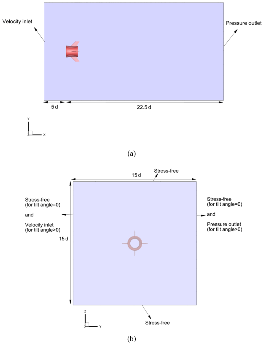
Figure 5 Size of the computational domain and boundary conditions by looking at the (a) x–y plane and the (b) z–y plane

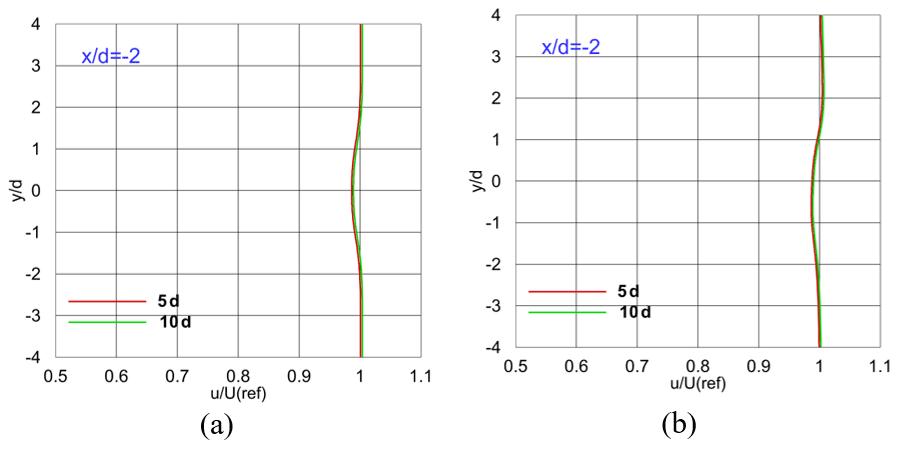
Figure 6 Comparison of vertical profiles of the time-averaged normalized x velocity for different upstream lengths for U_ref = 7 m s⁻¹, −4 < $y/d$ < 4, and z=0 with θ_tilt= (a) 0^∘ and (b) 10^∘ at $x/d$ = −2.

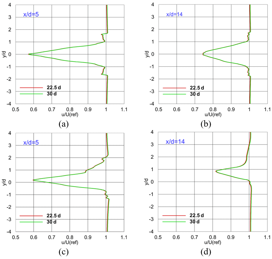
Figure 7 Comparison of vertical profiles of the time-averaged normalized x velocity for different downstream lengths for U_ref= 7 m s⁻¹, −4 $<y/d<\mathrm{4}$, and z=0 with θ_tilt= 0^∘ at (a) $x/d=$ 5, (b) $x/d=$ 14, and θ_tilt= 10^∘ at (c) $x/d=$ 5 and (d) $x/d=$ 14.

Saeed and Kim (2016) were the first to investigate the unsteady behavior of a helium-filled buoyant balloon without a rotor by employing computational fluid dynamics (CFD) and fluid–structure interaction (FSI) simulations. In another study (Saeed and Kim, 2017), they added a scaled NREL Phase IV rotor to the buoyant balloon and predicted the aerodynamic performance of the rotor at different wind speeds and yaw angles by using the K–omega shear stress transport (SST) model. Their results showed that the presence of the balloon can increase the output torque by 17 % compared to the bare turbine for the wind speed of 7 m s⁻¹. Recently, Ali and Kim (2020) attempted to consider the effects of wind shear, tilt, and yaw angle on the aerodynamic performance of a stand-alone rotor under wind conditions at 400 m altitudes and proved that both unsteady blade element momentum (UBEM) and CFD methods were reliable for calculating aerodynamic loads on rotor blades in airborne configuration, while the maximum amount of discrepancy between the methods did not exceed 4 %.

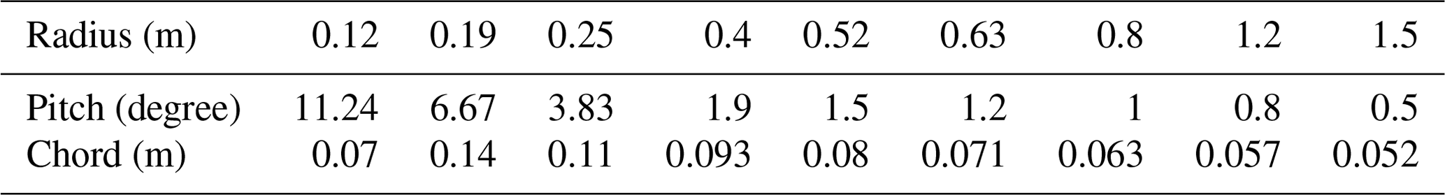
Table 1 Radial variation of the pitch angle and chord length for the turbine.

In all previous numerical studies on balloon wind turbines (Saeed and Kim, 2017, 2016; Ali and Kim, 2020), the K–omega SST turbulence model, a time-averaged model which assumes steady and homogeneous turbulence, has been adopted. In contrast, the high-fidelity large eddy simulation (LES) model has been widely used in conventional wind turbine wake studies to resolve the transient behavior of wake flows more accurately (Lin and Porté-Agel, 2019; Porté-Agel et al., 2011; Mo et al., 2013b, a). LES can resolve the large-scale turbulent motions that transport kinetic energy and momentum in wind turbine wakes. These large-scale motions are difficult to capture with Reynolds-averaged Navier–Stokes equations (RANS) simulations, which are better suited for smaller-scale turbulence. This is particularly important for wind turbine wake simulations, where the large-scale structures dominate the flow behavior (Churchfield et al., 2012; Yang and Sotiropoulos, 2013).

To resolve a wide range of turbulent motions using LES, it is necessary to use a fine mesh in regions of high turbulence, such as the boundary layers and wake regions (Pope, 2000). Hence, providing the required mesh for the rotor geometry and its boundary layer significantly increases total cell numbers and raises computational costs. On the other hand, using the actuator disk model (ADM) enables representing the turbine forces on airflow, needless to include the rotor geometry. Combining LES and ADM (LES–ADM) has emerged as a promising approach for predicting wind turbine wakes (Porté-Agel, 2011; Yang and Sotiropoulos, 2013; Stevens et al., 2018), which can capture unsteady flow features, such as vortex shedding and turbulent eddies, that are difficult to simulate using unsteady Reynolds-averaged Navier–Stokes equations (URANS)–ADM. Purohit et al. (2021) compared the LES–ADM and URANS–ADM for prediction of offshore wake losses against experimental results; they revealed that using LES–ADM in the wake simulation accounts for the more accurate forecast of turbulence intensity levels and velocity deficit in the wake region.

The LES–ADM is especially effective in predicting the flow variables in far wakes, where the flow is less turbulent and more uniform. Since the near-wake areas are characterized by large eddies, which can considerably raise the turbulence intensity of the flow, they are not considered suitable for placing subsequent arrays of wind turbines. Therefore, accurate prediction of far-wake behavior is critical for optimizing wind farms. In this regard, Lin and Porté-Agel (2019) studied the turbine wake characteristics using a hybrid ADM and LES model for an incoming wind with a yaw angle. Their result revealed an acceptable agreement with both wind-tunnel measurements and analytical wake models regarding wake deflections and spanwise profiles of the mean velocity deficit and turbulence intensity. According to previous studies, in this paper, the hybrid ADM–LES model based on the blade element momentum (BEM) theory is employed to predict the wake behavior of a balloon wind turbine and the aerodynamic forces acting on its balloon. Investigating the wake length behind these kinds of turbines is valuable as functioning in upstream turbines' wake flow means lower incoming wind speed, which leads to power losses and raises the oscillating loads on downstream rotor blades, shortening their lifetime (Porté-Agel, 2011).

Moreover, balloon wind turbines are considered non-crosswind systems among airborne wind energy systems (AWESs; Cherubini et al., 2015) and should be suspended at the specific altitude with preferred minimum displacement to perform in design conditions. The tethers attached to the balloon are responsible for its suspension and should balance the aerodynamic loads on the balloon. Consequently, studying the magnitude and behavior of the aerodynamic forces applied to the balloon in various wind conditions is essential to dynamics analysis and control issues. Thus, the results of this investigation can be applied to promote the efficiency of balloon wind turbine farms in an optimized layout and design a controlling system for them. Additionally, a criterion for adjusting the grid size in the wake region and around the balloon was used in this research to resolve 80 % of turbulent kinetic energy (TKE) in the wake directly in LES. Such a criterion has not been utilized to evaluate the grid size in the numerical study of the turbine wake so far (Porté-Agel, 2011; Porté-Agel et al., 2011; Lin and Porté-Agel, 2019; Mo et al., 2013b, a).

2 Computational model

Theoretically, a turbulence model called direct numerical simulation (DNS) can directly resolve the entire spectrum of eddies with wide ranges of time and length scales. However, this model demands high computational resources, especially for large domains and complex flows. Hence, different turbulence models have been developed by spatial averaging (Germano, 2000) and time averaging (Alfonsi, 2009) of Navier–Stokes equations to make an optimal trade-off between computational cost and accuracy. In LES, large eddies are resolved directly, and small eddies are filtered and modeled using secondary equations (Germano, 2000). Consequently, with respect to DNS, LES makes it possible to use a coarser mesh with a larger time step. The governing equations and assumptions used in this model can be obtained from Kim (2004). Since the dynamic Smagorinsky–Lilly model exhibited accurate results in the wake study of conventional wind turbines (Lin and Porté-Agel, 2019; Mo et al., 2013b; Porté-Agel et al., 2011), it was employed to predict the wake characteristics of balloon wind turbines in the current study.

3 Wind turbine modeling

The actuator disk model was used to model the rotor in this study. In this approach, the rotor is considered a rotating disk in the flow field, and the reaction forces of the rotor on air are obtained by employing the BEM. The rotating or actuator disk (AD) is the area swept by the turbine blades. The BEM calculates the mutual forces between the blade and the air by combining the momentum and blade element theory. In the following sections, these two methods are briefly explained, and, in the last section, the turbine's and the balloon's geometry are described.

3.1 Momentum theory

The schematic views of the control volume enclosing the AD and an annular element at the rotor plane are illustrated in Fig. 1. In this Fig. 1, r, U, and a represent element radius, air velocity, and the axial induction factor, respectively. The axial induction factor is the fractional difference in wind velocity between the free stream and the rotor plane.

Applying the conservation of linear and angular momentum to the control volume and the annular element and using the definition of induction factor a, thrust, dT can be computed by Eq. (1), and torque, dQ exerted on this element can be calculated from Eq. (2). In Eq. (2), $\stackrel{\mathrm{´}}{a}$ is the angular induction factor ($\stackrel{\mathrm{´}}{a}=\mathit{\omega }/\mathrm{2}\mathrm{\Omega }$).

$$\begin{array}{}\text{(1)}& {\displaystyle }\mathrm{d}T={\displaystyle \frac{\mathrm{4}a(\mathrm{1}-a)}{\mathrm{2}}}\mathit{\rho }{U}^{\mathrm{2}}\mathrm{2}\mathit{\pi }r\mathrm{d}r\text{(2)}& {\displaystyle }\mathrm{d}Q=\mathrm{4}\stackrel{\mathrm{´}}{a}(\mathrm{1}-a)\mathit{\rho }U\mathit{\pi }{r}^{\mathrm{3}}\mathrm{\Omega }\mathrm{d}r\end{array}$$

3.2 Blade element theory

In this approach, each rotor's blade is divided into N elements, as depicted in Fig. 2a. The relation between various forces, angles, and velocities at the blade is shown in Fig. 2b, looking down from the blade tip.

In Fig. 2b, dF_L is the lift force, dF_D is the drag force, dF_N is the force normal to the plane of rotation (which contributes to the thrust), and dF_T is the force tangent to the circle swept by the rotor. Considering a rotor with B blades, the total normal force, dF_N, on a section with radius r and thickness dr, can be computed from Eq. (3) using geometric relations between different forces in Fig. 2. In these equations C_l and C_d refer to lift and drag coefficients, respectively. Moreover, the total torque, dQ, exerted on this section can be estimated by multiplying dF_T by r as Eq. (4) :

$$\begin{array}{}\text{(3)}& {\displaystyle }\mathrm{d}{F}_{\mathrm{N}}=\stackrel{\mathrm{´}}{\mathit{\sigma }}\mathit{\pi }\mathit{\rho }{\displaystyle \frac{U^{\mathrm{2}}{\left(\mathrm{1}-a\right)}^{\mathrm{2}}}{{\sin }^{\mathrm{2}}\mathit{\phi }}}(C_{\mathrm{l}}\cos \mathit{\phi }+C_{\mathrm{d}}\sin \mathit{\phi })r\mathrm{d}r,\text{(4)}& {\displaystyle }\mathrm{d}Q=\stackrel{\mathrm{´}}{\mathit{\sigma }}\mathit{\pi }\mathit{\rho }{\displaystyle \frac{U^{\mathrm{2}}(\mathrm{1}-a{)}^{\mathrm{2}}}{{\sin }^{\mathrm{2}}\mathit{\phi }}}(C_{\mathrm{l}}\sin \mathit{\phi }-C_{\mathrm{d}}\cos \mathit{\phi })r^{\mathrm{2}}\mathrm{d}r,\end{array}$$

where ${\mathit{\lambda }}_{\mathrm{r}}=\frac{r\mathrm{\Omega }}{U}$ and $\stackrel{\mathrm{´}}{\mathit{\sigma }}=\frac{\mathrm{Bc}}{\mathrm{2}\mathit{\pi }r}$ are the local speed ratio and solidity, respectively.

By equating normal force (Eqs. 1 and 3) and torque (Eqs. 2 and 4) equations from the momentum and blade element theory, and after some algebraic manipulation, Eqs. (7)–(11) are gained. In these equations, F is Prandtl's tip loss factor and can be computed from Eqs. (5) and (6) (Hansen, 2015). And a_c=0.2 is the Glauert correction for the axial induction factors greater than 0.4.

$$\begin{array}{}\text{(5)}& {\displaystyle }F={\displaystyle \frac{\mathrm{2}}{\mathit{\pi }}}{\cos }^{-\mathrm{1}}\left(e^{-f}\right),\text{(6)}& {\displaystyle }f={\displaystyle \frac{B}{\mathrm{2}}}{\displaystyle \frac{R-r}{r\sin \mathit{\phi }}},\text{(7)}& {\displaystyle }{C}_{\mathrm{l}}=\mathrm{4}F\sin \mathit{\phi }{\displaystyle \frac{(\cos \mathit{\phi }-{\mathit{\lambda }}_{\mathrm{r}}\sin \mathit{\phi })}{\stackrel{\mathrm{´}}{\mathit{\sigma }}(\sin \mathit{\phi }+{\mathit{\lambda }}_{\mathrm{r}}\cos \mathit{\phi })}}\text{(8)}& {\displaystyle }\stackrel{\mathrm{´}}{a}={\displaystyle \frac{\mathrm{1}}{\frac{\mathrm{4}F\cos \mathit{\phi }}{\stackrel{\mathrm{´}}{\mathit{\sigma }}{C}_{\mathrm{l}}}-\mathrm{1}}},\text{(9)}& {\displaystyle }a={\displaystyle \frac{\mathrm{1}}{\frac{\mathrm{4}F{\sin }^{\mathrm{2}}\mathit{\phi }}{\stackrel{\mathrm{´}}{\mathit{\sigma }}{C}_{\mathrm{l}}\cos \mathit{\phi }}+\mathrm{1}}}a\le a_{\mathrm{c}},\text{(10)}& {\displaystyle }\begin{array}{rl}a=& {\displaystyle \frac{\mathrm{1}}{\mathrm{2}}}\left[\mathrm{2}+K\left(\mathrm{1}-\mathrm{2}{a}_{\mathrm{c}}\right)\right.\\ & \left.-\sqrt{(K\left(\mathrm{1}-\mathrm{2}{a}_{\mathrm{c}}\right)+\mathrm{2}{)}^{\mathrm{2}}+\mathrm{4}(K{a}_{\mathrm{c}}^{\mathrm{2}}-\mathrm{1})}\right]a>a_{\mathrm{c}},\end{array}\text{(11)}& {\displaystyle }K={\displaystyle \frac{\mathrm{4}F{\sin }^{\mathrm{2}}\mathit{\phi }}{\stackrel{\mathrm{´}}{\mathit{\sigma }}{C}_{\mathrm{l}}}}\end{array}$$

Since $\mathit{\phi }={\mathit{\theta }}_p+\mathit{\alpha }$, for a given blade geometry and operating conditions, there are two unknowns in Eq. (7), namely C_l and α per section. To find these values, one can use the empirical C_l versus α curves of the airfoil (Vries, 1979). One then finds C_l and α from the empirical data satisfying Eq. (7). Once C_l and α are known, $\stackrel{\mathrm{´}}{a}$ and a can be determined from Eqs. (8)–(11). After finding these values, the axial force and torque exerted on the blade section (equal to reacting forces on wind streams) can be obtained from Eqs. (3) and (4).

3.3 Turbine geometry

In this study, a turbine with 3 m diameter, d, and 0.75 m clearance from the inner surface of the balloon was used. The rotor comprises two blades and rotates around its horizontal axis with angular velocity Ω =251 rpm. The S809 airfoil, used in the NREL Phase VI rotor's blades, was selected for all blade sections. This rotor has shown good aerodynamic performance in wind turbine applications (Hand et al., 2001; Simms et al., 2001). Empirical curves of C_l and C_d versus α for this airfoil can be extracted from Airfoil Tools (2022). To calculate the optimized value of θ_P and c per section, the QBlade software was employed. In this optimization method, the angle of attack (AOA) was computed for each section using the tip speed ratio and Eq. (12).

$$\begin{array}{}\text{(12)}& \mathit{\alpha }={\tan }^{-\mathrm{1}}\left({\displaystyle \frac{\mathrm{2}}{\mathrm{3}}}{\displaystyle \frac{\mathrm{1}}{{\mathit{\lambda }}_{\mathrm{r}}}}\right)\end{array}$$

Optimize for lift/drag sets the twist at the specified λ_r at which the blade section operates to an AOA that yields the highest glide ratio ($C_{\mathrm{l}}/C_{\mathrm{d}})$. The optimized chord distribution was calculated by using Eq. (13) according to BETZ (Gasch and Twele, 2010):

$$\begin{array}{}\text{(13)}& c\left(r\right)={\displaystyle \frac{\mathrm{16}\mathit{\pi }r}{{\mathrm{BC}}_{\mathrm{L}}}}{\sin }^{\mathrm{2}}\left({\displaystyle \frac{\mathrm{1}}{\mathrm{3}}}{\tan }^{-\mathrm{1}}\left({\displaystyle \frac{R}{r{\mathit{\lambda }}_{\mathrm{r}}}}\right)\right).\end{array}$$

Radial variations of the chord length and pitch angle are presented in Table 1.

To model the effects of the hub on wind streams, a cylinder with the radius of 0.08 m and drag coefficient of $C_{\mathrm{d},\mathrm{hub}}=\mathrm{1.2}$ was used according to Churchfield et al. (2015). The axial aerodynamic force exerted from the hub can be calculated from Eq. (14). In this equation, R_hub and U_hub represent the hub radius and average wind speed at the hub height, respectively. After calculating all the aerodynamic forces by using AD and hub properties (Eqs. 3, 4, and 14), they were employed as sources of momentum in the domain by developing user-defined function (UDF) codes in ANSYS-FLUENT.

$$\begin{array}{}\text{(14)}& F_{\mathrm{hub}}={\displaystyle \frac{\mathrm{1}}{\mathrm{2}}}\mathit{\rho }\mathit{\pi }{R}_{\mathrm{hub}}^{\mathrm{2}}{U}_{\mathrm{hub}}^{\mathrm{2}}{C}_{\mathrm{d},\mathrm{hub}}\end{array}$$

3.4 Balloon geometry

A schematic representation of the turbine's balloon is shown in Fig. 3a. The balloon consists of a duct and four wings and is suspended by tethers. NACA 9414 airfoil was used in the duct cross-section to increase the wind speed passing the turbine (Saleem and Kim, 2018). To improve the stability of the balloon in strong winds, four wings with n0009sm-il airfoil cross-sections were attached to the duct (Saeed and Kim, 2016). The geometric dimensions of the balloon and the actuator disk (AD) position inside it are presented in Fig. 3b. As noted in this figure, the AD was located in the duct's throat to experience higher wind speed.

4 Computational domain

A cuboid domain was created around the balloon in the current study. To ensure zero gradients of flow variables on the boundaries, the upstream length, downstream length, and width of the cuboid domain were determined as 5, 22.5, and 15 times of the turbines' diameter, respectively. These dimensions are illustrated in Fig. 5. Unsteady simulations of the balloon wind turbine were performed with inlet reference velocity, U_ref= 7, 10, and θ_tilt= 0, 5 and 15^∘ to compare the behavior of the wake in various wind flow scenarios. For the non-tiled cases, only one inlet along the x axis was considered. However, in the tilted cases, a secondary flow was entered into the domain along the y axis to ensure the full exposure of the balloon wind turbine to the tilted wind stream (Fig. 5b). The velocity boundary condition was employed at the inlet(s) of the domain, while the pressure boundary condition was specified at the outlet(s). No-slip and stress-free walls were assigned to the balloon body and side walls of the domain, respectively.

Figure 8 Cells size around a (a) resolved eddy and (b) modeled eddy.

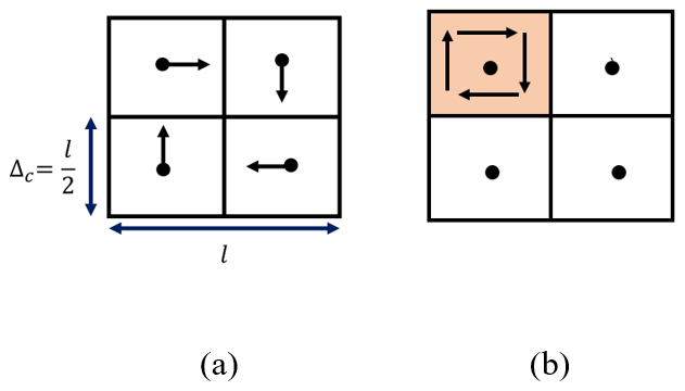
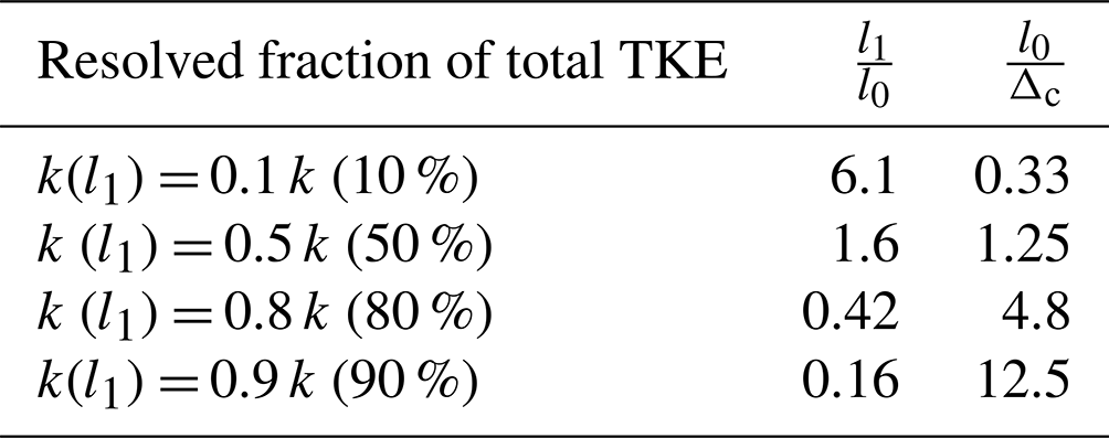
Table 2 The relation between k (l₁), l₁, and Δ_c based on Kolmogorov's energy spectrum.

Figure 9 Zone A, B, and C and the corresponding TEC diagrams.

For all the wind scenarios in this study, the altitude of 400 m was assumed. The corresponding air density and viscosity at this altitude were set to ρ=1.179 kg m⁻³ and $\mathit{\mu }=\mathrm{1.8}\times {\mathrm{10}}^{-\mathrm{5}}$ kg m⁻¹s⁻¹, respectively. The PISO scheme was utilized for pressure–velocity coupling. This scheme is well-suited for unsteady and highly transient flows, which are characteristic of wind turbine wake simulations. For spatial discretization of pressure and momentum, the second-order form and, for the time integration, the second-order implicit were employed to improve the stability and convergence of the simulations. Simulations ran for a maximum of 20 iterations per time step, using a convergence criterion of $\mathrm{1}\times {\mathrm{10}}^{-\mathrm{4}}$ for the residuals in all cases. Obtaining convergence in unsteady wind turbine wake simulations is time-consuming. To expedite the convergence process while maintaining stability, under-relaxation techniques, including the application of factors of 0.3 to the pressure equation and 0.7 to the momentum equation, were employed. The size of the time step was selected after sensitivity studies to assess the impact of the time step size on the convergence. The maximum time step required for the simulations to converge was selected, which was approximately close to the time required for a rotor rotation of 2.5^∘ (Δt = 0.0016 s). LES calculations were run sufficiently to reach stable statistics of the flow. In other words, after passing this criterion, the time-averaged flow variables have not experienced significant changes. On this basis, the simulation time was set at approximately 9.2 s, corresponding to 40 rotations of the rotor. The 1333 sampling data during this time were taken to perform the time-averaging process on the flow variables.

To assess the impact of the computational domain size on the results, simulations were performed separately using two distinct domain sizes: one with an extended upstream length (from 5 to 10d) and the other one with an extended downstream length (from 22.5 to 30d) relative to the turbine position. The number of nodes was increased by a factor of 2 in the extended upstream domain's upstream distance and by 1.3 times (equal to the length increment ratio) in the extended downstream domain's downstream distance to ensure consistent spatial resolution in all cases while only considering the influence of changes in computational domain size on the results. The simulations were performed for U_ref= 7 m s⁻¹ and θ_tilt= 0 and 10^∘. Figures 6 and 7 illustrate the results as vertical profiles of the time-averaged normalized x velocity at different locations within the range of −4 < $y/d$ < 4 at z = 0 for extended upstream and downstream length domains, respectively.

According to Fig. 6, extending upstream length has been observed to have a relatively minor impact on the velocity profiles at the upstream location. This observation can be attributed to the specific study conditions, particularly the placement of the balloon wind turbine at a high altitude with a more stable atmosphere, less affected by surface heating and friction, resulting in reduced turbulence and vertical mixing. The absence of significant boundary layer effects due to the high-altitude location of the turbine led to a longer upstream length less critical for capturing boundary layer-related phenomena. These specific environmental conditions allowed for the design of a computational domain with a smaller upstream length than is typically required to study the wake behavior of ground-based wind turbines. Furthermore, as shown in Fig. 7, prolonging the downstream distances has shown only a marginal influence on the velocity profiles at different positions relative to the turbine location. The downstream domain size was designed to encompass the essential characteristics of the wake, including wake recovery, turbulence decay, and gradual mixing with ambient air. Under these controlled conditions and with careful attention to factors critical to wake simulation, the impact of extending the domain size upstream and downstream remained minimal, demonstrating the suitability of the selected computational domain size.

5 Grid generation

5.1 Mesh resolution in LES

LES requires mesh sizes sufficiently fine to resolve the energy-containing eddies. The mesh resolution determines the fraction of TKE directly resolved. In this study, a method was adopted to generate a mesh that could directly resolve about 80 % of the local TKE spectrum in the wake flow and the region enclosing the balloon. Moreover, the entire domain was discretized with hexahedral elements using ANSYS-ICEM. In the following, the concepts and equations of this approach are described.

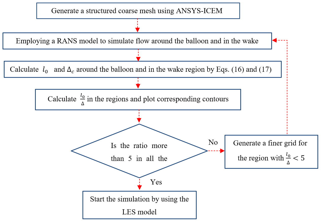
Figure 10 The steps in generating mesh to resolve 80 % of total TKE around the balloon and in the wake.

According to Fig. 8a, resolving an eddy with diameter l requires four cells with the width of $l/\mathrm{2}$ (=Δ_c). However, if the width of two adjacent cells around the eddy is less than $l/\mathrm{2}$, as shown in Fig. 8b, this eddy cannot be resolved directly, and the sub-grid-scale models will be used to resolve it.

Figure 11 Mesh topology around the balloon.

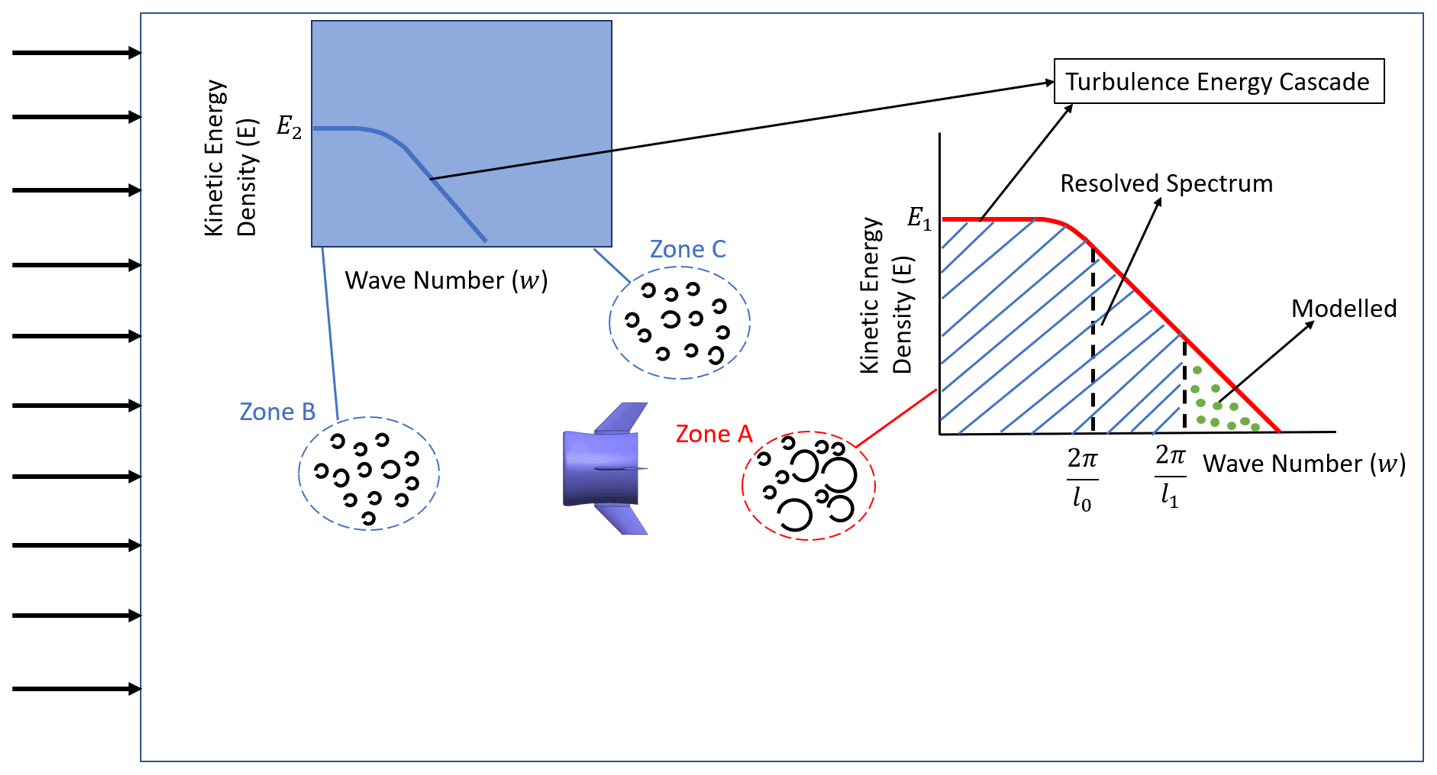
A schematic view of the eddies downstream of the turbine in three zones (A, B, and C) and their corresponding turbulence energy cascade (TEC) diagrams are depicted in Fig. 9. While zone A is located in the wake flow, zones C and B are far from the wake region. TEC diagrams in Fig. 7 represent the relation between the wave number of eddies, $w(=\mathrm{2}\mathit{\pi }/l$), and their kinetic energy density, E. According to these diagrams, as the length scale (diameter) of eddies decreases, their wave number w increases while their kinetic energy density declines. Considering the location of zone A in the turbulent wake region, the length scale of eddies and their kinetic energy density in this region are higher (E₁>E₂) than those of zones B and C.

Table 3 Mesh distribution in the computational domain for evaluating mesh criterion in LES.

In Fig. 7, more details of the TEC diagram in zone A are described. The area under the TEC curve indicates the total TKE of all eddies in this zone. The smallest size of the resolved eddies is considered to be l₁. The area under the TKE curve for eddies smaller than l₁ (the dotted area) is modeled, while that of greater sizes (the crosshatched area) is directly resolved via LES.

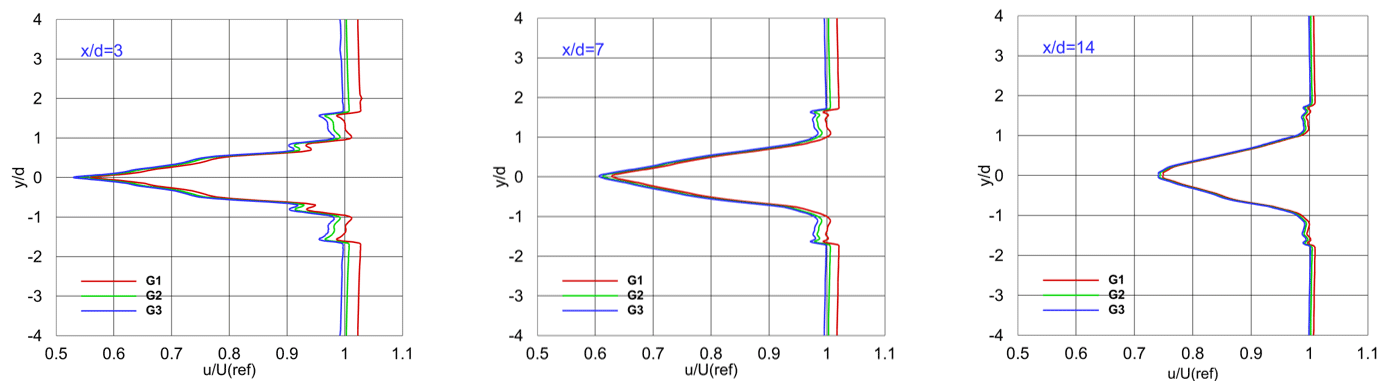
Figure 12 Vertical profiles of the time-averaged normalized x velocity at different locations downstream of the turbine.

All eddies in each arbitrary region can be equated with an eddy with l₀ length scale called integral length scale (ANSYS, 2016). This eddy contains the averaged energy of all the eddies in the determined region, and its size can be computed from Eq. (15), in which k represents the TKE of an eddy with wave number w.

$$\begin{array}{}\text{(15)}& {\displaystyle \frac{l_o}{\mathrm{2}\mathit{\pi }}}={\displaystyle \frac{{\int }_{\mathrm{0}}^{\mathrm{\infty }}{w}^{-\mathrm{1}}k\left(w\right)l\left(w\right)}{{\int }_{\mathrm{0}}^{\mathrm{\infty }}k\left(w\right)l\left(w\right)}}\end{array}$$

Table 2 presents the relation between the resolved fraction of total TKE (dotted area in Fig. 9, k(l₁)), l₁, and cell size, Δ_c, based on the Kolmogorov's energy spectrum (ANSYS, 2016). Here, l₀ and Δ_c can be calculated from Eqs. (16) and (17). In these equations, ε and V represent the dissipation rate of the TKE and cell volume, respectively. According to this table, to resolve about 80 % of the total TKE in a region, there should be at least five cells along l₀. To resolve this amount of TKE in the wake flow and around the balloon, an algorithm was used to obtain the mesh size. Different steps of the algorithm are shown in Fig. 10.

$$\begin{array}{}\text{(16)}& {\displaystyle }{l}_o={\displaystyle \frac{k^{\left(\frac{\mathrm{1}}{\mathrm{3}}\right)}}{\mathit{\epsilon }}}\text{(17)}& {\displaystyle }{\mathrm{\Delta }}_{\mathrm{c}}=V^{\left(\frac{\mathrm{1}}{\mathrm{3}}\right)}\end{array}$$

According to Fig. 10, a coarse mesh was generated in ANSYS-ICEM at the beginning of each simulation. In the following step, a precursor RANS simulation was performed to estimate l₀ and Δ_c around the balloon and in the wake region from Eqs. (26) and (27). The K–omega SST model was employed in the precursor simulations, utilizing simulation setup and boundary conditions similar to that of the main models. The K–omega SST model accurately estimates turbulence kinetic energy and dissipation by employing a dual-equation formulation, which captures the interactions between these quantities more comprehensively. Additionally, its enhanced near-wall treatment improves accuracy in capturing boundary layer characteristics, making it a reliable choice for precise calculations. Next, the contours of $l_{\mathrm{0}}/\mathrm{\Delta }$ were plotted to check the mesh resolution in these regions. When $l_{\mathrm{0}}/\mathrm{\Delta }$ was smaller than 5 in specified regions, the first mesh was refined, and the process was continued from step 2; otherwise, the LES simulation was started using the first mesh.

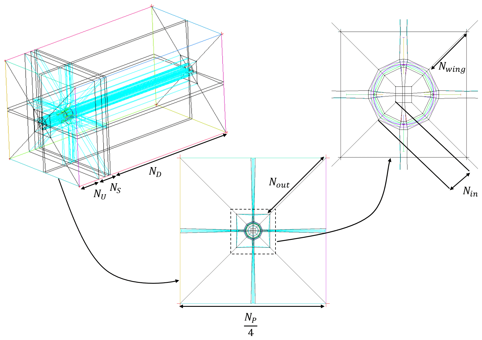
5.2 Blocking method and mesh independence study

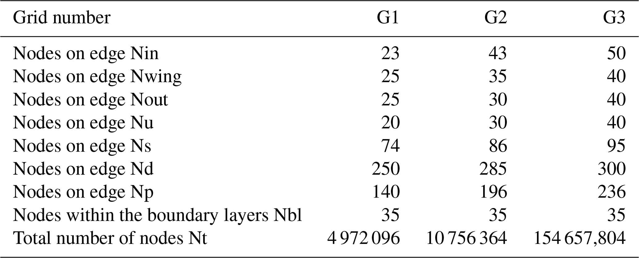
To discretize the cuboid computational domain by hexahedral elements, it was divided into three regions along its axial axis (upstream, downstream, and chord length of the balloon), as shown in Fig. 11. Next, the four O-grid topologies were used to split these blocks in the radial direction to control the mesh inside and in the width of the duct, wings, and the region around the balloon. To accurately capture the boundary layer effects, the value of y+ was set to approximately 1, and 20 inflation layers were assigned with a growth ratio of 1.2 in the direction normal to the walls. Mesh distribution in the domain using the criterion was named mesh G2, and its details are given in Table 3.

To further assess the criterion, its grid independence was investigated. Accordingly, two coarser (G1) and finer (G3) meshes, summarized in Table 3, were generated. By employing these meshes in three simulations, a comparison was conducted on the vertical profiles of the time-averaged normalized x velocity at three distinct downstream locations. All of the simulations were performed for U_ref= 10 m s⁻¹ and θ_tilt= 0^∘, and the results are illustrated in Fig. 12.

According to Fig. 12, using a coarser grid in the near wake leads to a lower prediction of velocity deficit. This is because as the grid size grows, the small-scale turbulence structures and vortices are not accurately resolved. As a result, the flow tends to smooth out, and the turbulence effects are underestimated. This can lead to an underprediction of the velocity deficit in the near wake. However, the difference in average velocity at 3d downstream of the turbine between mesh G3 and G2 is about 1 %, while this difference is around 4 % for meshes G2 and G1. Moreover, the difference between velocity profiles for different grids decreases in further regions. Since the discrepancy between G2 and G1 mesh results is about one-fourth of the difference between G2 and G3, the mesh criterion in LES satisfies the wake recovery's mesh independence requirement. All the simulations were performed by high-performance computing (HPC) systems having GPUs to accelerate the calculation time.

Figure 13 depicts the mesh on the balloon; two perpendicular planes pass through it, with a magnified view of the boundary layer's mesh. Evidently, the boundary layers' mesh thoroughly covered the walls to improve the accuracy in calculating viscous forces.

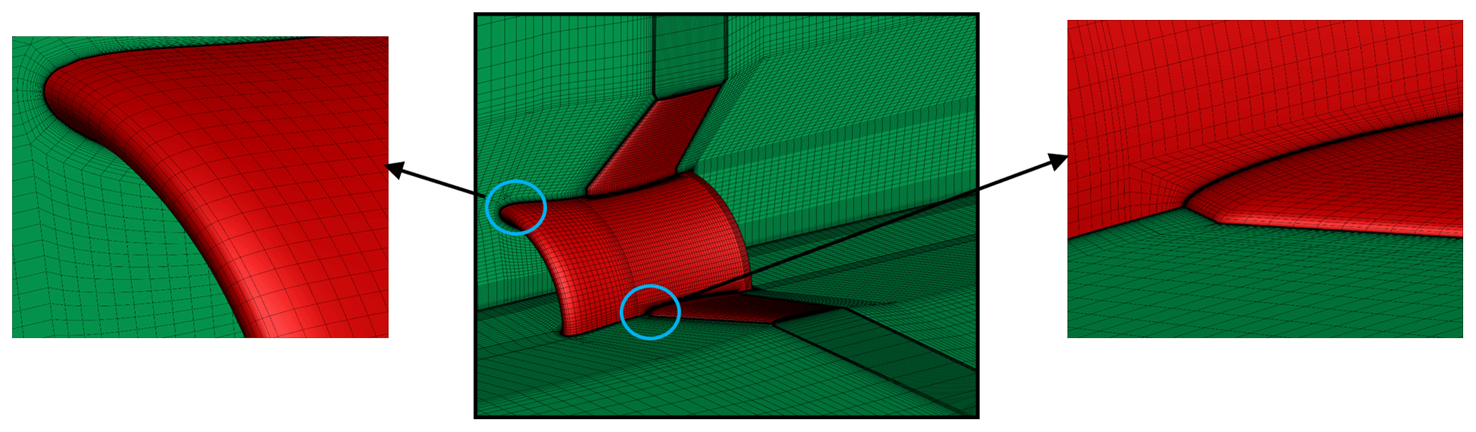
Figure 13 Mesh distribution on the balloon body, two perpendicular planes passing through, and an exaggerated view of mesh in the boundary layers of one wing and the duct.

6 Results and discussions

6.1 Validation of simulation

Since balloon wind turbine systems are novel research topics, experimental data regarding wake analysis were unavailable to validate the results of the current study. To assess the capabilities of the hybrid ADM-LES model and the mesh criterion in LES, the wake behavior of a smaller conventional turbine (functioning on the ground) was studied, which had been studied experimentally before (Chamorro and Porté-Agel, 2010). The corresponding turbine diameter and angular velocity were 1.5 cm and 1220 rpm, respectively. An unsteady simulation was run for 50 s flow time to obtain stable time-averaged flow statistics. The position of AD and the location of one upwind line and seven downwind lines of the turbine ($x/d$ = −1, 2, 3, 5, 7, 10, 14, 20) for 0 < $y/d<\mathrm{2}$ at the symmetry plane of the channel (z=0) are illustrated in Fig. 14. The cubic domain was discretized with 192, 32, and 42 nodes along the x and y axes. At the end of the simulation, the time-averaged streamwise velocity at these locations was calculated and compared with those from the experimental study in Fig. 15.

In Fig. 15, the boundary layer effects can be observed on the exponential upwind profile. Looking at downstream profiles in Fig. 15, a good agreement between the experimental measurements and the ADM–LES method is observed for all the locations. The results showed that the numerical model can accurately predict the non-unform velocity deficit in the near and far wake. Deviation of the numerical results from wind tunnel measurement at $x/d=\mathrm{2}$ close to the ground can be justified since the tower effects were neglected in the numerical investigation. The maximum velocity deficit occurs at the hub height. Moreover, the wake effects can be seen until $x/d=\mathrm{20}$, where the time-averaged streamwise velocity profile is at its primary shape due to momentum extraction from the free stream.

Figure 14 The location of selected lines in upwind and downwind of the turbine.

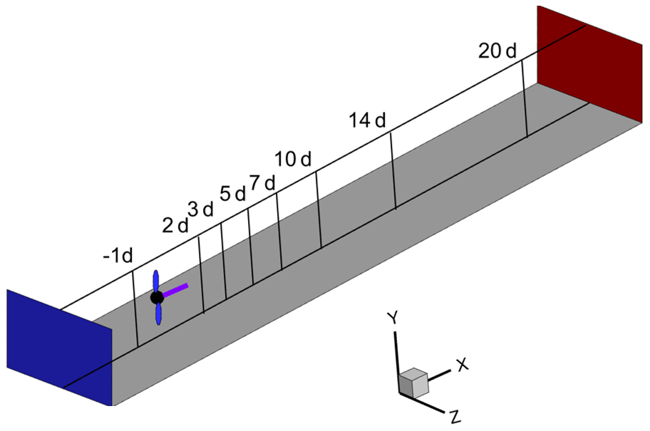
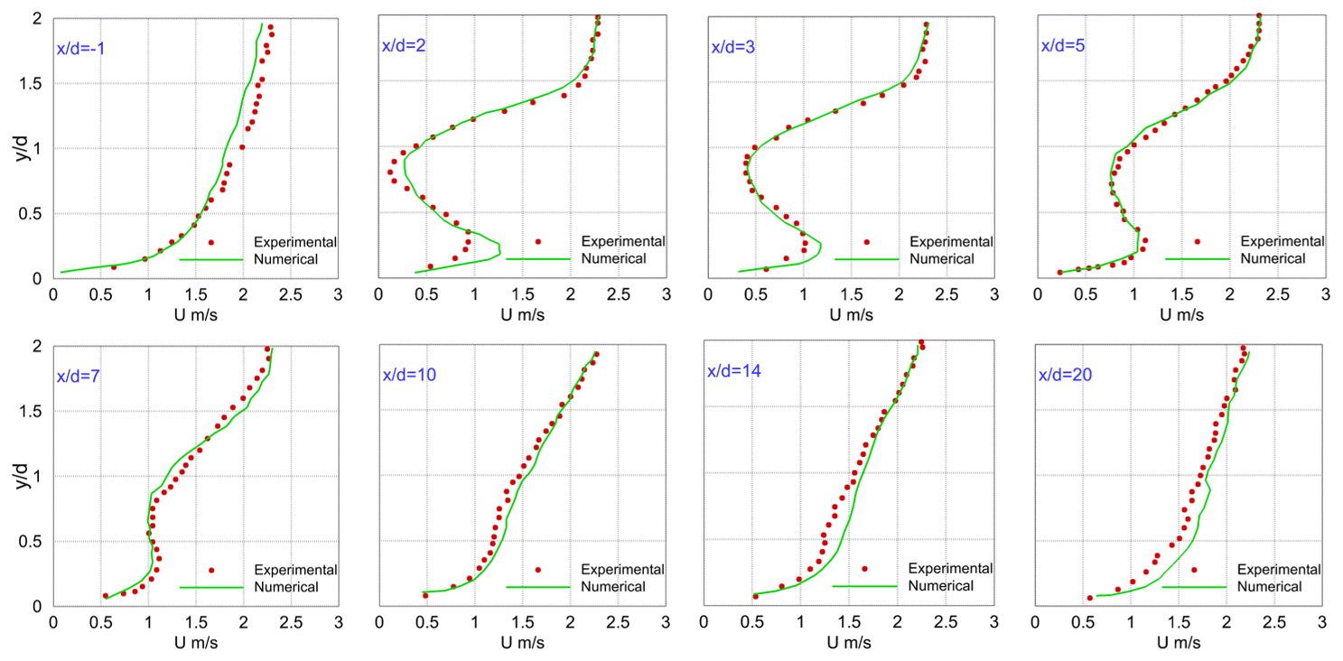
Figure 15 Comparison of vertical profiles of the time-averaged streamwise velocity U (m s⁻¹): ADM–LES (solid line) and wind-tunnel measurements (dotted line).

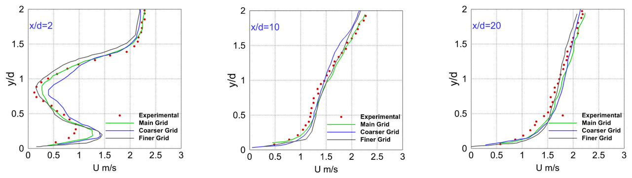
Figure 16 Comparison of vertical profiles of the time-averaged streamwise velocity U (m s⁻¹) obtained by the experimental study and simulations with different grids.

To assess the grid independence of velocity profiles in the wake, the simulations were performed for a coarser and finer mesh. The number of nodes in the coarser and finer grids along the x, y, and z directions was 120 × 25 × 30 and 250 × 50 × 60, respectively. Figure 16 shows the comparison of vertical profiles of the time-averaged streamwise velocity obtained from the experimental study and three different grids. According to Fig. 16, decreasing the grid size slightly affects the velocity profiles, particularly within the far wake, and the results obtained from the main grid demonstrate good consistency with experimental measurements.

6.2 Velocity profiles in the balloon wind turbine wake

In this section, the results of the wake analysis of the balloon wind turbine are reported and discussed. Figure 17 displays the vertical profiles of the time-averaged normalized x velocity for one upstream and seven normalized downstream locations behind the turbine for −4 $<y/d<$ 4 at z=0. For a better understanding of the wake behavior in different wind scenarios, various incoming velocities (U_ref= 7 and 10 m s⁻¹) and different tilt angles (θ_tilt= 0, 5 and 10^∘) were used. In Fig. 17, the stagnation effects of the turbine on the incoming air are apparent on upwind profiles in all the cases.

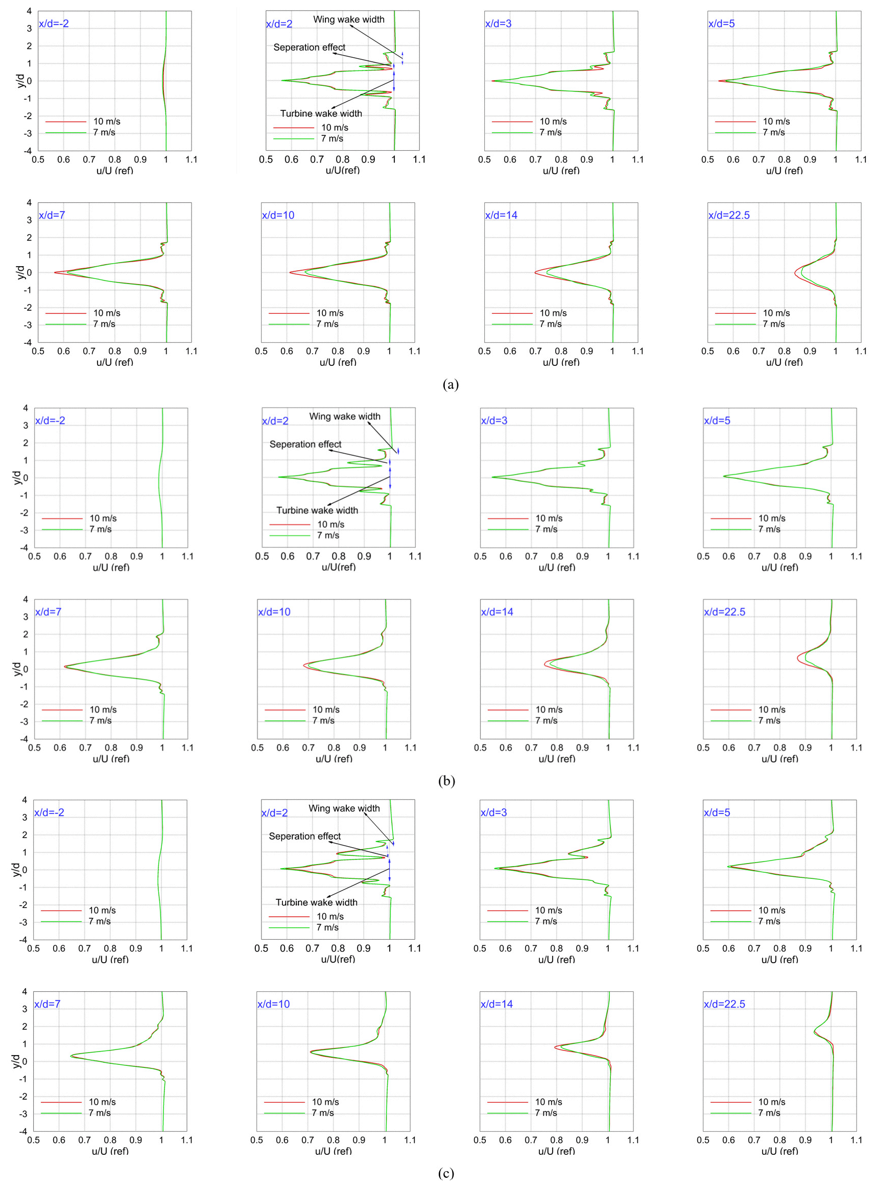
Figure 17 Comparison of vertical profiles of the time-averaged normalized x velocity for one upstream and seven downstream locations for −4 $<y/d<$ 4 at z=0 in θ_tilt= (a) 0^∘, (b) 5^∘, and (c) 10^∘.

These effects lead to the 1 % velocity deficit for the regions −2.1 $<y/d<$ 2.1, −2.3 $<y/d<$ 1.3, and −2.5 $<y/d<$ 1.1 at θ_tilt= 0, 5, and 10^∘, respectively. On the other hand, there is clear evidence of velocity deficit in three regions just when the airflow passes through the balloon. These regions contribute to rotor wake, wing wake, and separation effects in the trailing edge of the duct's airfoil. The wake structures in these three regions are investigated separately below.

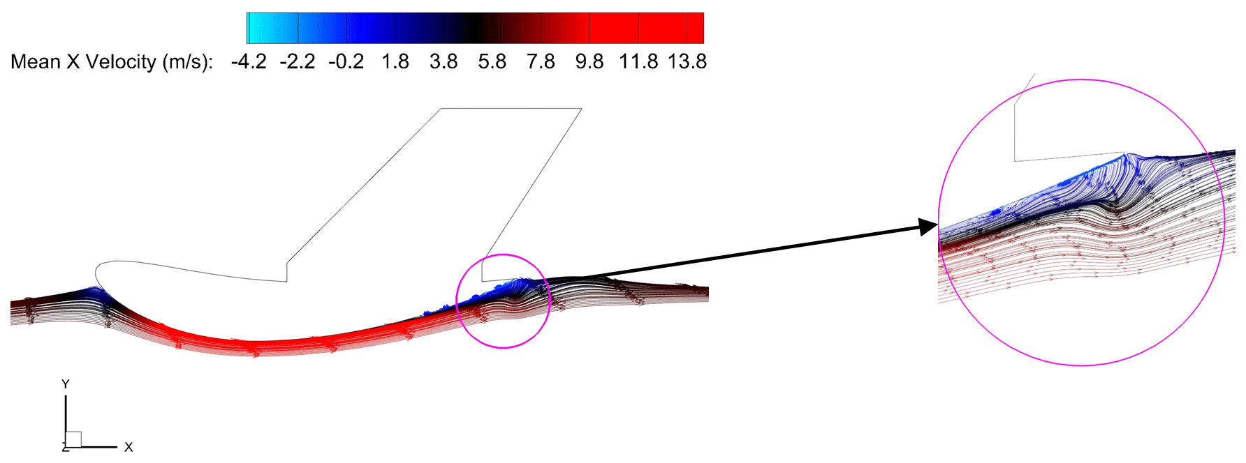
Figure 18 Separated streamlines near the trailing edge of the duct's airfoil for U_ref= 7 m s⁻¹ and θ_tilt= 5^∘ at the symmetry plane of the balloon (z=0).

According to Fig. 17a, the normalized x-velocity profiles for U_ref= 7 m s⁻¹ are quite similar to U_ref= 10 m s⁻¹ everywhere in the wake. However, at U_ref = 7 m s⁻¹, relatively faster recovery can be observed in the rotor wake. It can be explained by the higher value of tip speed ratio (TSR) for U_ref= 7 m s⁻¹ at the same rotational speed leading to increased shear turbulence in the wake, as observed in other studies (Krogstad and Adaramola, 2012; Martínez-Tossas et al., 2022). Higher shear turbulence in the wake can cause more lateral turbulent diffusion into the region and, consequently, faster recovery (Krogstad and Adaramola, 2012; Martínez-Tossas et al., 2022). The difference in the recovery rate is noticeable up to $x/d=\mathrm{10}$, where the difference in the averaged x velocity in the wake width is maximized at 6 % for the two wind speeds.

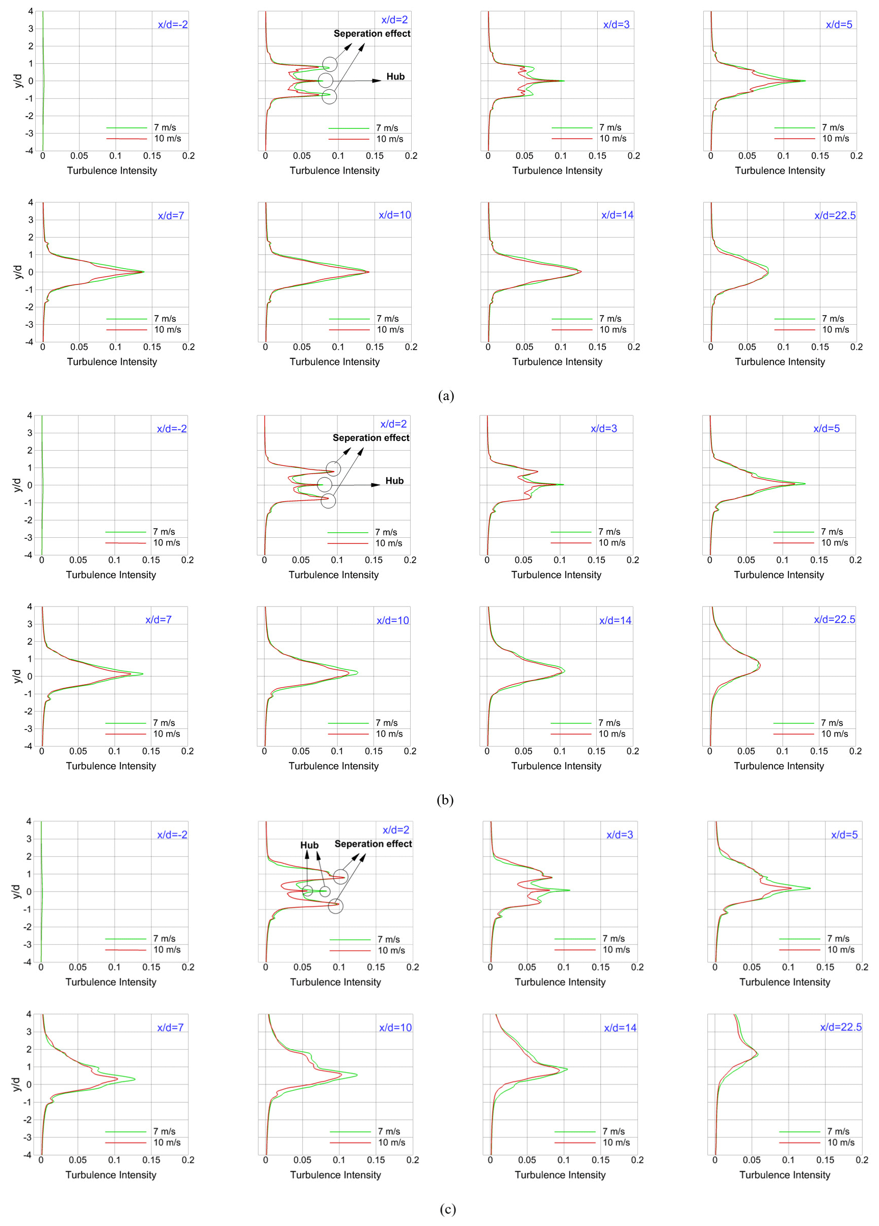
Figure 19 Comparison of vertical profiles of the time-averaged turbulence intensity for one upstream and seven downstream locations for −4 $<y/d<$ 4 at z=0 in θ_tilt= (a) 0^∘, (b) 5^∘, and (c) 10^∘.

The effect of tilt angle on wake behavior is depicted in Fig. 17b and c. Irrespective of the incoming wind speed, it can be observed that the wake is deflected toward the tilted direction as the tilt angle increases. Moreover, the wake becomes asymmetric around the rotor axis compared with the non-tilted inflow, and the wake center (location of the minimum velocity) shifts upward in the lateral direction as the wake progresses further downstream. By increasing θ_tilt, there is a reduction in the wake width of the rotor for locations far from $x/d=\mathrm{7}$. This reduction can be attributed to two reasons. Firstly, by increasing the tilt angle, there is less interaction between the wind flow and the rotor because of a decrease in the rotor swept area, as seen from the incoming flow, which provides less momentum to be extracted by the rotor. Secondly, as the tilt angle increases, there is an increment in the supply of momentum from the surrounding free stream into the wake. As a result, the velocity deficit in the wake recovers faster. Hence, the time-averaged x velocity in the wake width at $x/d=\mathrm{22.5}$ reaches 0.93, 0.94, and 0.96 of the free-stream value for θ_tilt= 0, 5, and 10^∘, respectively.

Comparing the results of tilted and non-tilted inflow in Fig. 17, it can be interpreted that the effect of tilt angle on momentum transformation into the wake is stronger than TSR as there is a slight difference in velocity profiles for different U_ref in Fig. 17b and c. The wake width reduction and deflection may be desirable in increasing the incoming wind speed of any downstream balloon wind turbine in wind farms. Therefore, tilt angle and TSR are essential factors in designing an optimized layout of wind farms for balloon wind turbines.

Considering the velocity profiles just after the turbine ($x/d=\mathrm{2}$) in Fig. 17, there is evidence of velocity defect due to the presence of the wings. However, the wings' effect on the velocity field is not as significant as the effects of separation. It should be claimed that, in all wind scenarios investigated in this study, the wings did not experience the stall phenomenon, and no separation was observed around them, which can justify their negligible effect on the velocity field. According to Fig. 17, the wings' effect on flow disappears at distances as large as $x/d=\mathrm{14}$ in all the cases. The third distinct region in the wake structure in Fig. 17 is related to the separation effect in the trailing edge of the duct's airfoil. Figure 18 shows streamlines near the trailing edge of the duct's airfoil for U_ref= 7 m s⁻¹ and θ_tilt= 5^∘ at the symmetry plane of the balloon (z=0). From this figure, the growing rate of the duct cross-section after the throat generates a positive pressure gradient in the streamwise direction, which leads to flow separation in the boundary layer of the duct's inner surface.

6.3 Turbulence intensity profiles in the balloon wind turbine wake

Similar to conventional wind farms on the ground, turbulence intensity (TI $=u^{\prime }/U)$ is a key factor in studying wind farms of balloon wind turbines. From one viewpoint, high turbulence intensity in the airflow can amplify the frequency of aerodynamic loads on blades, which may adversely affect rotor dynamics and shorten the blade's lifetime (Ismaiel and Yoshida, 2018). On the other hand, when the frequency of the oscillations approaches the system's natural frequency, a resonance phenomenon may happen, which leads to high-amplitude oscillations and affects the balloon's stability. In this regard, vertical profiles of the time-averaged turbulence intensity for locations mentioned above in the previous wind scenarios are illustrated in Fig. 19. As is evident from the figure, the presence of the balloon wind turbine does not increase TI in the incoming upstream flow. On the other hand, right after the flow passes through the balloon, it experiences a noticeable TI increment in two distinct regions. The first region's width is equal to the diameter of the rotor at −0.5 $<y/d<$ 0.5. The TI growth in this region is related to large-scale vortices generated by the angular momentum transformation of the actuator disk, which moves downstream in the wake. The second region is related to flow separation in the trailing edge of the duct's airfoil (Fig. 18). Vortices in this region can promote TI along the duct's width (−0.8475 < $y/d$ < −0.66 and 0.66 $<y/d<$ 0.8475).

From Fig. 19, higher TI can be observed at all the tilt angles at U_ref= 7 m s⁻¹ and almost everywhere downstream of the turbine. This is due to higher shear turbulence in the wake of higher TSR cases, as described in the previous section. It is observed that in the case of θ_tilt= 0^∘ and U_ref= 7 m s⁻¹, TI is higher than 10 m s⁻¹ until $x/d=\mathrm{10}$, which can explain faster recovery for U_ref= 7 m s⁻¹ up to $x/d=\mathrm{10}$ as observed in Fig. 17a. By increasing the tilt angle in Fig. 19b and c, the TSR difference between two incoming wind speeds will grow with a coefficient of $\mathrm{1}/\cos \left({\mathit{\theta }}_{\mathrm{tilt}}\right)$, which explains the greater TI difference than the non-tilted inflow.

From Fig. 19, TI in the rotor wake (−0.5 $<y/d<$ 0.5) for θ_tilt= 0, 5, and 10^∘ gradually increases until $x/d=\mathrm{10}$, 7, and 5, respectively, and then starts to fall. This reduction can be attributed to the instability of the wake flow and the breakdown of large-scale vortices (eddies) into smaller vortices in these locations. When large-scale eddies flow downstream in the wake, their energy will be transferred into smaller eddies; in the smallest scales, this energy is converted into the internal energy of the flow. The results show that the energy cascade or the transfer of energy from large-scale motions to small-scale ones in this region continues at distances as large as $y/d=\mathrm{22.5}$. However, in the region attributed to separation effects, the energy cascade continues up to $x/d=\mathrm{5}$ for θ_tilt= 0 and 5^∘; then, the maximum TI remains below 5 % further downstream. Note that, at θ_tilt= 10^∘, vortices generated by the rotor and the separation are merged, and their effects are significant even at 10 d downstream of the turbine.

6.4 Aerodynamic loads on the balloon

Figure 20 shows a schematic view of the resultant aerodynamic forces and the resultant torques exerted on the balloon. As shown in this figure, the system has 6 degrees of freedom, demanding complex control systems. Several tethers are connected from the base station to the balloon responsible for controlling the system. These tethers should be connected at specific points and directions on the balloon to balance aerodynamic forces and prevent high increments of yaw and tilt angles. Studies on the control and dynamic model of the system are outside the scope of the current study and may be the subject of future research. In this section, aerodynamic forces acting on the balloon are numerically investigated by employing the LES–ADM method for the same wind scenarios used in previous sections. Total aerodynamic forces are divided into pressure forces and viscous forces. The magnitude of these forces in x (drag forces) and y directions (lift forces) are plotted in Fig. 21. Considering no inflow along the z axis from boundaries into the domain and the symmetrical geometry of the balloon about the x–y plane, the resultant force in this direction is nearly zero for all the cases (R_Z=0).

Figure 20 A schematic of aerodynamic loads on the balloon.

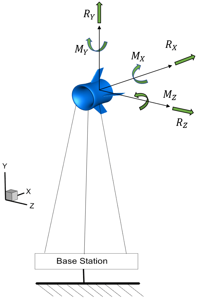
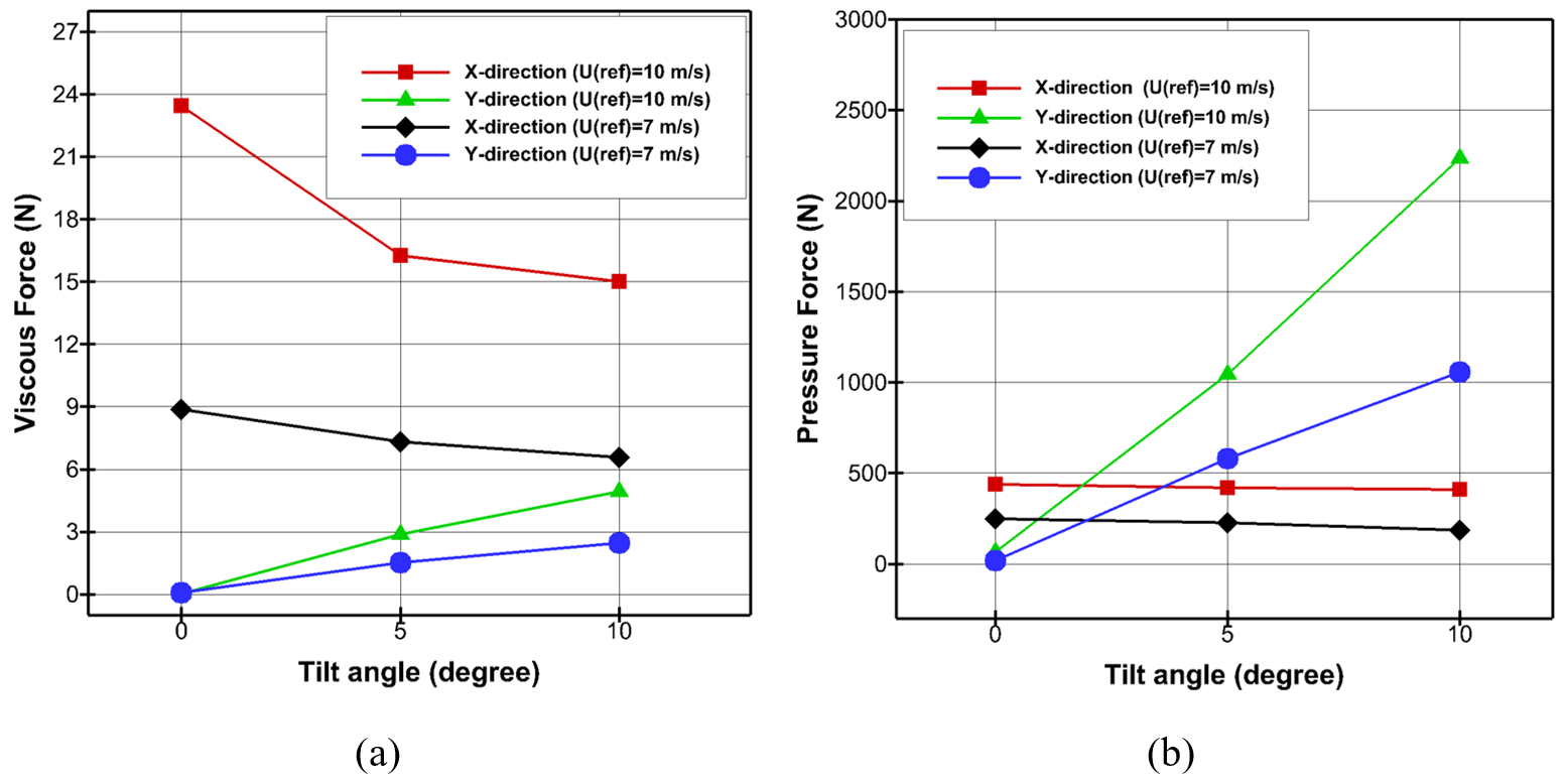
Figure 21 (a) Viscous forces and (b) pressure forces on balloon in the x- and y-direction variation with wind speeds and tilt angles.

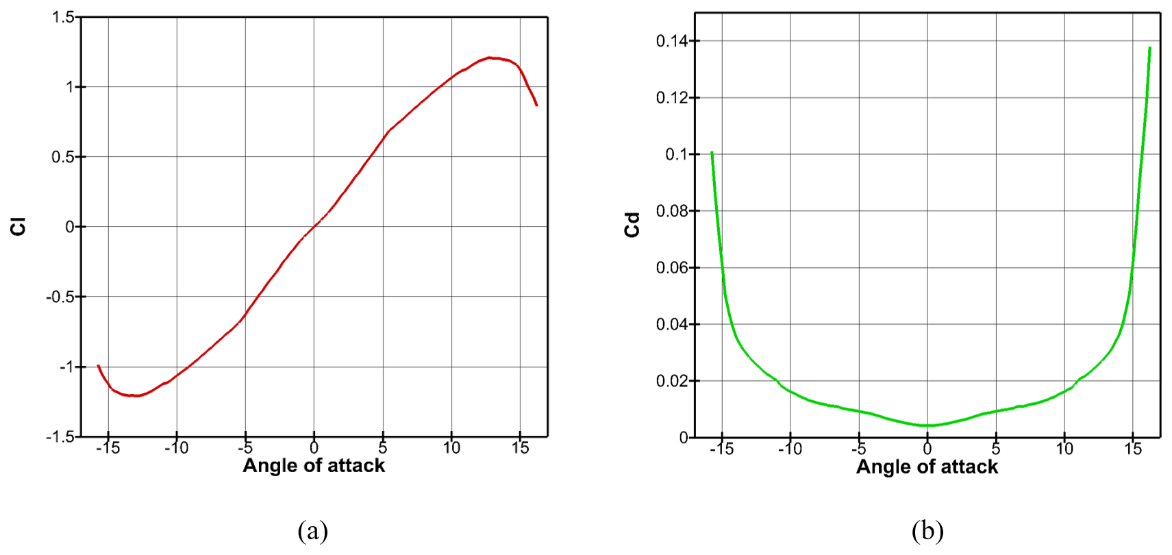
Figure 22 (a) Lift coefficient and (b) drag coefficient versus angle of attack in 7 m s⁻¹ wind speed.

From Fig. 21a, it can be seen that with increasing θ_tilt to 10^∘, viscous forces in the y direction increase marginally to 5 N for U_ref= 10 m s⁻¹ and decrease to about 6 N for U_ref= 7 m s⁻¹ in the x direction. This trend may be due to the increment of the y component and reduction of the x component of incoming flow when the tilt angle rises. As displayed in Fig. 21b, pressure forces in the y direction have a direct relation with tilt angle, and they reach 1055 and 2235 N for U_ref= 7 and 10 m s⁻¹, respectively, at θ_tilt= 10^∘. On the other hand, the magnitude of the pressure forces slightly decreases in the x direction when the tilt angle rises, but they always remain under 500 N in all wind scenarios. It should be pointed out that, for tilted inflows, pressure forces are always higher in the y direction. The lower order of viscous forces relative to pressure forces was predictable and was approved by the results.

For a better understanding of the relation of these forces with tilt angle and wind speed, aerodynamic loads on the duct and wings should be analyzed separately. Figure 22 shows C_l and C_d versus the AOA (tilt angle in the current study) for the wings' cross-section airfoil at U_ref= 7 m s⁻¹. Since the airfoil has a symmetric profile, the corresponding lift coefficient is zero and the drag coefficient is very low (about 0.004) at θ_tilt= 0^∘. According to the figure, a stall occurs when the AOA exceeds 13^∘, which is above the maximum tilt angle in all the cases used in the current study.

In Fig. 22, all the wings are named, and the magnitudes of aerodynamic forces acting on wing Wh1 are plotted in different directions. Regarding θ_yaw= 0^∘, there is a symmetric velocity field around wings Wv1 and Wv2, which generates very low magnitudes of lift and drag forces by considering Fig. 22. Furthermore, due to the symmetric flow pattern about the x–y plane, vectors of resultant forces on wings Wh1 and Wh2 are equal. As wing Wh1 operates below the stall angle, the corresponding lift force experiences a rise as the tilt angle increases, which is evident from Fig. 23b. In addition, the magnitude of the lift force at θ_tilt= 10^∘ is 73 N for U_ref= 7 m s⁻¹ and 146 N for 10 m s⁻¹. By comparing Figs. 21 and 23c, the portion of the lift forces exerted on the wings in the total lift force exerted on the balloon can be calculated. Hence, this value was measured to be around 12 % and 14 % for U_ref= 7 and 10 m s⁻¹, respectively, at θ_tilt= 5^∘. At θ_tilt= 10^∘, it experiences a rise being almost 28 % for U_ref= 7 m s⁻¹ and 29 % for U_ref= 10 m s⁻¹. It can be concluded that, by increasing the tilt angle, the ratio of the lift force on the wings to the total lift force on the balloon will increase; therefore, a controlling system is required for balancing such extra lift force.

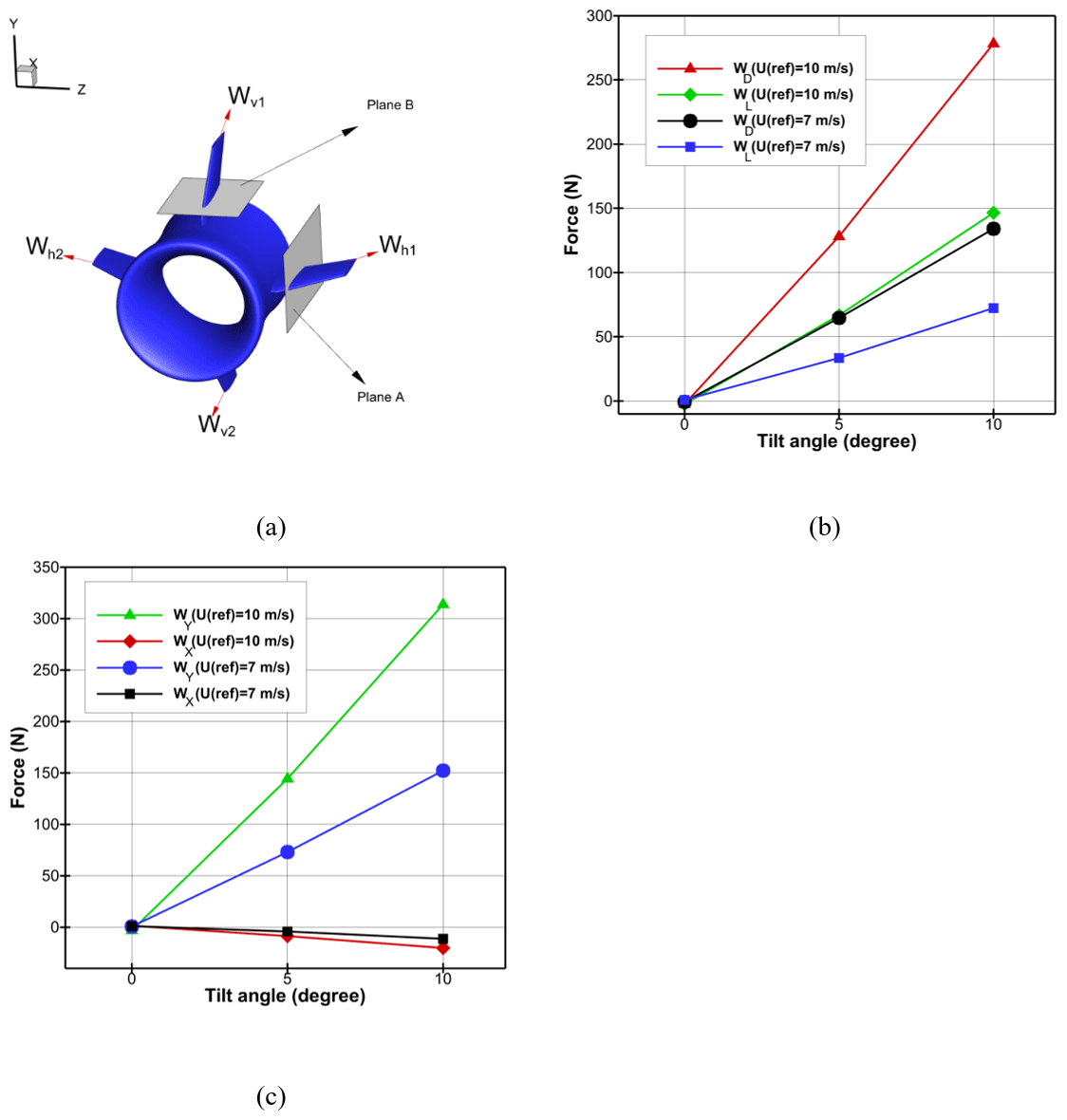
Figure 23 (a) Wings' names, (b) lift and drag forces on wing Wh1, and (c) projection of the corresponding forces in the x and y directions in different wind scenarios.

In Fig. 24a, pressure contours on the inner and outer surfaces of the right surface of the duct are presented for U_ref= 7 m s⁻¹ and θ_tilt= 0^∘. Taking into account the symmetric flow and geometry concerning the x–y plane, the resultant aerodynamic forces on both sides are equal in the y direction. As shown in the figure, the pressure on the outer side of the surface is higher than that of the inner side in different areas, except for the area near the leading edge. Therefore, the pressure difference generates a resultant force toward the center of the balloon. In Fig. 24b, a schematic representation of these resultant forces is shown on two separate airfoils (A1 and A2) at different circumferential positions on the duct (−β and β around the x axis). As the airfoils are symmetric about the x–z plane, aerodynamic forces exerted on them are equal in magnitude at θ_tilt= 0^∘, (F_R2)_Y=(F_R1)_Y, but they act in opposite directions. Therefore, the total lift force on the right surface (and the lift surface) is zero in the non-tilted inflow. However, for the tilted inflows, the pressure distributions on the pressure side of these airfoils and on the suction side are not the same; consequently, (F_R2)_Y≠(F_R1)_Y, which can generate a lift force on the duct.

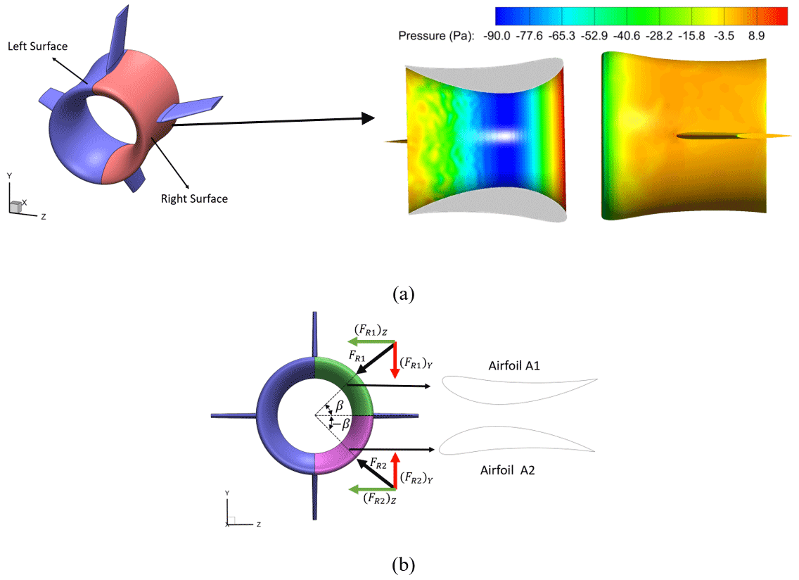
Figure 24 (a) Pressure contour on the inner and outer surfaces of the right surface of the duct in U_ref= 7 m s⁻¹ and θ_tilt= 0^∘. (b) Schematic of the resultant forces on two separate airfoils in different circumferential positions on the duct (−β and β around x axis).

Figure 25 illustrates the time-averaged pressure coefficient for A1 and A2 airfoils in the streamwise direction at β= 30, 45, and 60^∘. The mean C_P in this figure was calculated at U_ref= 7 m s⁻¹ and θ_tilt= 10^∘. From the figure, there is an obvious difference in mean C_P at each normalized distance for different values of β. This discrepancy is due to different pressure distributions on their pressure and suction sides for tilted inflows, as described before. Consequently, for tilted inflows, (F_R2)_Y>(F_R1)_Y, and the balloon will experience an aerodynamic lift force in addition to the buoyant force, which can help the system float in the air.

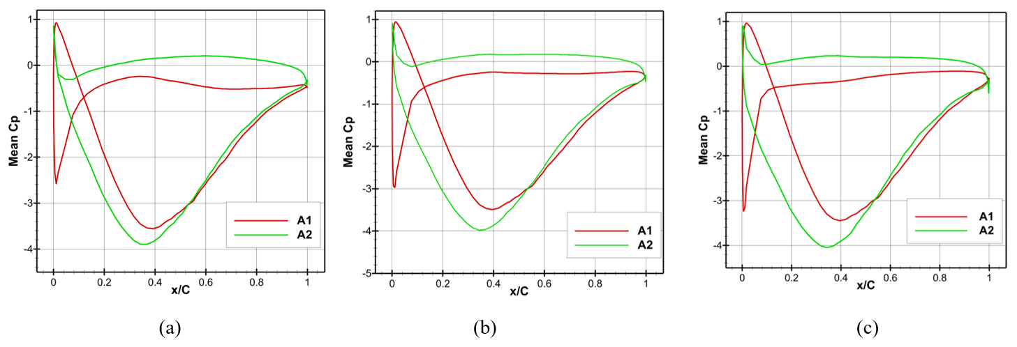
Figure 25 Mean C_P for A1 and A2 airfoils in streamwise direction for U_ref= 7 m s⁻¹ and θ_tilt= 10^∘ in (a) β= 30^∘, (b) β= 45^∘, and (c) β= 60^∘.

7 Conclusions

The wake characteristics and aerodynamics of a balloon wind turbine were numerically investigated for different wind scenarios by employing a hybrid LES–ADM model. A mesh criterion was used to resolve more than 80 % of TKE in the wake and around the balloon. The conclusions drawn from the results of this study are as follows:

1. The mesh generated by using the aforementioned criterion and the proposed algorithm satisfied mesh independence requirements.

2. The wake structure of the balloon wind turbine consisted of three distinct regions affected by the wings, rotor, and separation in the trailing edge of the duct's airfoil. For non-tilted inflows, higher TSR led to faster momentum recovery in the wake at distances as large as 10d from the turbine. However, by increasing the tilt angle, the effect of this parameter on the wake recovery was reduced and the wake shifted toward the tilted direction. It was concluded that both TSR and tilt angle are essential factors in designing an optimized layout of a balloon wind turbine farm.

3. When the airflow passed through the balloon, it experienced a rise in two distinct regions affected by the separation along the duct's width (−0.8475 $<y/d<$ −0.66 and 0.66 $<y/d<$ 0.8475) and the wake behind the rotor (−0.5 $<y/d<$ 0.5). The TI in the rotor wake rose until 10, 7, and 5d downstream for θ_tilt= 0, 5, and 10^∘, respectively. In these locations, vortices generated by the rotor broke down into smaller eddies and, consequently, TI declined.

4. In the region corresponding to separation, energy transformation to smaller eddies continued up to 5d downstream for θ_tilt= 0, 5^∘, and the maximum TI in this region remained below 5 % in further downstream locations. However, at θ_tilt= 10^∘, eddies generated by the separation and rotor were merged, and their effect remained significant at distances as large as 10d from the rotor.

5. An upward trend was observed for the lift force versus tilt angle such that, at θ_tilt = 10^∘, it reached 1055 and 2235 N for incoming wind speeds of 7 and 10 m s⁻¹, respectively. Furthermore, as the tilt angle increased, the portion of the wings' lift in the total balloon's lift reached 29 % at θ_tilt= 10^∘, which was recognized as an important factor in the controlling system design of the balloon.