An analytical linear two-dimensional actuator disc model and comparisons with computational fluid dynamics (CFD) simulations

The continuous up-scaling of wind turbines enabled by more lightweight and flexible blades in combination with coning has challenged the assumptions of a plane disc in the commonly used blade element momentum (BEM)-type aerodynamic codes for the design and analysis of wind turbines. The objective with the present work is thus to take a step back relative to the integral 1-dimensional (1-D) momentum theory solution in the BEM model in order to study the actuator disc (AD) flow in more detail.

We present an analytical, linear solution for a two-dimensional (2-D) AD flow with one equation for the axial velocity and one for the lateral velocity, respectively. Although it is a 2-D model, we show in the paper that there is a good correlation with axis-symmetric and three-dimensional (3-D) computational fluid dynamics (CFD) simulations on a circular disc. The 2-D model has thus the potential to form the basis for a simple and consistent rotor induction model.

For a constant loading, the axial velocity distribution at the disc is uniform as in the case of the classical momentum theory for an AD. However, an important observation of the simulated flow field is that immediately downstream of the disc the axial velocity profiles change rapidly to a shape with increased induction towards the edges of the disc and less induction on the central part. This is typically what is seen at the disc in full non-linear CFD AD simulations, which is what we compare with in the paper.

By a simple coordinate rotation the analytical solution is extended to a yawed disc with constant loading. Again, a comparison with CFD, now with a 3-D simulation on a circular disc in yaw, confirms a good performance of the analytical 2-D model for this more complicated flow.

Finally, a further extension of the model to simulate a coned disc is obtained using a simple superposition of the solution of two yawed discs with opposite yaw angles and positioned so the two discs just touch each other. Now the validation of the model is performed with results from axis-symmetric CFD simulations of an AD with a coning of both 20 and −20^∘. In particular, for the disc coned in the downwind direction there is a very good correlation between the simulated normal velocity to the disc, whereas some deviations are seen for the upwind coning.

The promising correlation of the results for the 2-D model in comparison with 3-D simulations of a circular disc with CFD for complicated inflow like what occurs at yaw and coning indicates that the 2-D model could form the basis for a new, consistent rotor induction model. The model should be applied along diagonal lines on a rotor and coupled to an angular momentum model. This application is sketched in the outlook and is a subject for future research.

1 Introduction

The most striking characteristic of the modern, industrial wind turbine development over the last 4–5 decades is the up-scaling. In the beginning of the 1980s there was already an industrial series production of turbines with a rated power of 50–100 kW and rotor diameters of 15–20 m. Many were installed in big wind farms like Palm Springs and Tehachapi in the United States. Today turbines of the maximum size of around 15 MW with rotor diameters of 230–240 m have been introduced in the market, which gives an up-scaling factor of around 15 on rotor diameter over this time span.

It is clear that this up-scaling correspondingly increased the requirements for the aerodynamic and aeroelastic design tools like the modelling of unsteady inflow over the rotor disc, wind shear and wind veer, yawed flow, and wake flow (Madsen et al., 2020). The origin of the aerodynamic modelling of the common aeroelastic model tools today – like FLEX5 (Flex4) (Øye, 1996), FAST (Jonkman et al., 2016), BLADED (Bossanyi, 2003), GAST (Riziotis and Voustinas, 1997), Cp-Lambda (Botasso et al., 2006), FOCUS (WMC, 2019) and HAWC2 (Larsen and Hansen, 2007) – is the blade element momentum (BEM) theory based on the propeller theory by Glauert (1935) which originally assumed homogeneous and stationary flow. Various modifications have been implemented in the different codes to adapt to the conditions mentioned above. Most codes, e.g., now use a more local representation of the induction over the rotor plane than on a ring element as originally proposed to better account for varying inflow over the rotor disc from wind shear and turbulence.

An excellent overview of the capability of most of the above-mentioned codes has recently been presented by Boorsma et al. (2023). This was done by both bench-marking and validation of experimental data as well as of higher-fidelity model data. One conclusion is that the BEM-type codes still show higher deviations for yawed inflow than higher-fidelity codes like computational fluid dynamics (CFD) and vortex-type codes. For yawed flow cases the variability between BEM-type codes is double the variability between CFD codes. This illustrates the lack of a unified implementation of the sub-models in BEM-type codes, e.g., for the modelling of yaw.

The objective with the present work is thus to take a step back relative to the integral momentum theory solution for an actuator disc, which is the core of the BEM model. We will study the actuator disc (AD) flow in more detail to provide a better background for understanding the shortcomings and approximations in the BEM-implemented momentum theory and deviations from higher-fidelity modelling of AD flow such as (1) the velocity distribution at the disc for constant loading, (2) independence of annular stream tubes, (3) flow field for a yawed AD and (4) flow field for a coned AD.

With respect to the axial velocity distribution for a constant loaded AD where the integral momentum theory predicts (assumes) a uniform, constant profile, a number of CFD-based AD simulations have shown higher induction towards the edges of the disc and less induction on the central part (Sørensen and Kock, 1995; Madsen, 1997; Mikkelsen et al., 2001). Also the shortcomings of the momentum theory to predict the flow through a coned rotor have been illustrated by CFD AD simulations of Madsen and Rasmussen (1999) and Mikkelsen et al. (2001), where considerable deviations from the constant axial velocity profile assumed by the momentum theory are found.

Studies within these four areas have been carried out by many researchers in the past, and it seems that the modelling can be grouped into three approaches: (1) vortex models, (2) combined analytical and numerical models, and (3) Euler-equation-based models which the present model belongs to.

The approach based on vortex models is by far the most common way of studying the AD flow field and not least the use of a vortex cylinder (VC) model with a none-expanding wake, infinite number of blades, infinite tip speed ratio and uniform loading. Some recent studies in relation to the above-mentioned research areas using this model are Branlard and Gaunaa (2015) (relations between momentum theory and vortex theory), Li et al. (2022) (modelling of non-planar rotors), Troldborg et al. (2014) (yawed disc), and Gaunaa et al. (2023) (independence of annular stream tubes).

In the category of studies combining analytical and numerical solutions Crawford (2006) presented a modified BEM for coned rotors. The improvement in the BEM model comprises a proper consideration of the relative placement of the wake and includes the radial-induced velocity. A comparison of the improved BEM with the CFD results of Madsen and Rasmussen (1999) and Mikkelsen et al. (2001) shows reasonable correlation as concerns the slope of the profiles on the inner part of the disc, whereas the non-linear outboard part required a further modelling of the expansion of the stream tubes.

Another study by van Kuik and Lignarolo (2016) shows the non-uniformity of the axial velocity profile caused by the pressure acting at the stream tube annuli, thus making them not independent from each other in contradiction to the independence found by Gaunaa et al. (2023). Finally in this group of models the work by Wood and Hammam (2022) can be mentioned, who used conservation of axial and angular momentum and the calculus of variations to derive the optimal performance of horizontal-axis wind turbines over a wide range of tip speed ratios. In the two-dimensional (2-D) model to be presented here the analytical solution is limited to a constant loading.

In the third model group, the Euler equations and the continuity equation together with specified body forces are the starting point for modelling the AD flow. It seems to be a unique approach, and only the so-called asymptotic acceleration potential method by van Bussel (1992) has some resemblance to the method used in the present research.

It might be considered surprising to study a 2-D AD model for the representation of rotor induction. However, it is expected that the main difference between an axis-symmetric and a 2-D model will be related to the analogy between radial velocity and lateral velocity for the axis-symmetric and 2-D model, respectively, where the last mentioned is expected to have the highest velocities.

The model and the background for its derivation are presented in Sect. 2 followed by flow characteristics of the AD model in axial flow in Sect. 3, including comparisons with axis-symmetric CFD simulations. Section 4 extends the model to yawed inflow and the validation with three-dimensional (3-D) CFD AD simulations. Section 5 presents a further extension for modelling a coned disc and comparisons with axis-symmetric CFD AD simulation of a disc with both 20 and −20^∘ coning. Outlook and conclusions are given in Sects. 6 and 7, respectively.

2 The analytical 2-D AD model

The analytical linear solution (2D_l) of the 2-D AD model was first presented by Madsen (1983) during a work on the development of the actuator cylinder (AC) model for modelling the aerodynamics of vertical-axis wind turbines (VAWTs). The basic idea behind the AC model was the need to extend the well-known actuator disc concept to an actuator surface (AS) of arbitrary shape where the AS coincides with the swept surface of the considered turbine type (Madsen, 1983, 1985, 1988). For a straight-bladed VAWT rotor this means a cylindrical shape which thus can be modelled with the AC model.

However, this extension of the AD concept to an AS raised the question of how to compute the flow field through and around an AS. The well-known momentum theory solution in an integral form for an AD cannot just be transferred for use on an AS of arbitrary shape, which would violate the assumptions in the AD momentum model.

2.1 Derivation of the descriptive system of equations

We have chosen an approach for the derivation of the equations that follows a general method of Von Kármán and Burgers (1935) for the analysis of flow fields with a main velocity V under the influence of external body forces f. Von Kármán and Burgers (1935) used the method to develop a general theory for wings of finite span and considered in most cases the induced velocities from the action of external forces as perturbations to the main flow field with the velocity V.

Koning (1935) presented an analysis of the flow around “the ideal propeller” described as a thin disc with axial forces acting over the disc, which is based on the method of Von Kármán and Burgers (1935) and thus also forms the basis for the present work. However, Koning (1935) studied the axis-symmetric flow problem, where we here will stick to a 2-D flow. The reason to focus on the 2-D flow case is that, as we will see later, a complete and simple analytical solution can be derived, which gives valuable and relevant insight into different flow features, whereas Koning (1935) for the analysis of the axis-symmetric case had to introduce approximations or assumptions, e.g., that the pressure solution found along the centre line of the disc was assumed to be valid at other radial positions. As we also will see later, the 2-D AD flow has characteristics resembling the 3-D AD flow and thus the potential to form the basis for a wind turbine rotor induction model. Furthermore the simple approach to model a coned rotor with two yawed disc is a big advantage of the 2-D model.

It should be noted that the full 3-D set of equations for the flow around an arbitrary 3-D AS has been presented by Madsen (1985) and Madsen (1988).

2.1.1 The full non-linear 2-D solution

The approach for derivation of the descriptive system of equations is based on the Euler equations on differential form and the equation of continuity with the external body forces f specified on the AD. Assuming steady flow the 2-D Euler equations take the following form:

$$\begin{array}{}\text{(1)}& {\displaystyle }{v}_x{\displaystyle \frac{\partial v_x}{\partial x}}+v_y{\displaystyle \frac{\partial v_x}{\partial y}}=-{\displaystyle \frac{\mathrm{1}}{\mathit{\rho }}}{\displaystyle \frac{\partial p}{\partial x}}+{\displaystyle \frac{\mathrm{1}}{\mathit{\rho }}}{f}_x,\text{(2)}& {\displaystyle }{v}_x{\displaystyle \frac{\partial v_y}{\partial x}}+v_y{\displaystyle \frac{\partial v_y}{\partial y}}=-{\displaystyle \frac{\mathrm{1}}{\mathit{\rho }}}{\displaystyle \frac{\partial p}{\partial y}}+{\displaystyle \frac{\mathrm{1}}{\mathit{\rho }}}{f}_y,\end{array}$$

and the equation of continuity is as follows:

$$\begin{array}{}\text{(3)}& {\displaystyle \frac{\partial v_x}{\partial x}}+{\displaystyle \frac{\partial v_y}{\partial y}}=\mathrm{0}.\end{array}$$

Following the approach by Von Kármán and Burgers (1935) we rewrite the velocity components as

$$\begin{array}{}\text{(4)}& {\displaystyle }{v}_x=V+w_x,\text{(5)}& {\displaystyle }{v}_y=w_y.\end{array}$$

Here V is the velocity of the main, uniform flow field; w_x and w_y the induced velocities by the action of the body forces; and v_x and v_y the final velocity components.

We then non-dimensionalize the velocity components with V, the pressure p with V²ρ, and volume forces f_x and f_y with V³ρ. However, although we now have non-dimensionalized the equations, the notation of velocity, body force components and pressure will not be changed.

Inserting the new velocity component notation and the non-dimensionalization into Eqs. (1), (2) and (3) and rearranging, we get

$$\begin{array}{}\text{(6)}& {\displaystyle \frac{\partial w_x}{\partial x}}=-{\displaystyle \frac{\partial p}{\partial x}}+f_x-\left(w_x{\displaystyle \frac{\partial w_x}{\partial x}}+w_y{\displaystyle \frac{\partial w_x}{\partial y}}\right),\text{(7)}& {\displaystyle \frac{\partial w_y}{\partial x}}=-{\displaystyle \frac{\partial p}{\partial y}}+f_y-\left(w_x{\displaystyle \frac{\partial w_y}{\partial x}}+w_y{\displaystyle \frac{\partial w_y}{\partial y}}\right),\end{array}$$

and the continuity equation

$$\begin{array}{}\text{(8)}& {\displaystyle \frac{\partial w_x}{\partial x}}+{\displaystyle \frac{\partial w_y}{\partial y}}=\mathrm{0}.\end{array}$$

Following the terminology of Von Kármán and Burgers (1935), the terms in the brackets on the right-hand side of Eqs. (6) and (7) can be interpreted as induced or second-order forces g_x and g_y, defined as

$$\begin{array}{}\text{(9)}& {\displaystyle }{g}_x=-\left(w_x{\displaystyle \frac{\partial w_x}{\partial x}}+w_y{\displaystyle \frac{\partial w_x}{\partial y}}\right),\text{(10)}& {\displaystyle }{g}_y=-\left(w_x{\displaystyle \frac{\partial w_y}{\partial x}}+w_y{\displaystyle \frac{\partial w_y}{\partial y}}\right).\end{array}$$

Inserting Eqs. (9) and (10) into Eqs. (6) and (7), we get

$$\begin{array}{}\text{(11)}& {\displaystyle \frac{\partial w_x}{\partial x}}=-{\displaystyle \frac{\partial p}{\partial x}}+f_x+g_x,\text{(12)}& {\displaystyle \frac{\partial w_y}{\partial x}}=-{\displaystyle \frac{\partial p}{\partial y}}+f_y+g_y.\end{array}$$

Now we take the divergence of Eqs. (11) and (12):

$$\begin{array}{}\text{(13)}& {\displaystyle \frac{{\partial }^{\mathrm{2}}{w}_x}{\partial x^{\mathrm{2}}}}=-{\displaystyle \frac{{\partial }^{\mathrm{2}}p}{\partial x^{\mathrm{2}}}}+{\displaystyle \frac{\partial f_x}{\partial x}}+{\displaystyle \frac{\partial g_x}{\partial x}},\text{(14)}& {\displaystyle \frac{{\partial }^{\mathrm{2}}{w}_y}{\partial x\partial y}}=-{\displaystyle \frac{{\partial }^{\mathrm{2}}p}{\partial x\partial y}}+{\displaystyle \frac{\partial f_y}{\partial y}}+{\displaystyle \frac{\partial g_y}{\partial y}}.\end{array}$$

Differentiating the equation of continuity Eq. (8) with respect to x and inserting Eqs. (13) and (14), we get

$$\begin{array}{}\text{(15)}& {\displaystyle \frac{{\partial }^{\mathrm{2}}p}{\partial x^{\mathrm{2}}}}+{\displaystyle \frac{{\partial }^{\mathrm{2}}p}{\partial y^{\mathrm{2}}}}=\left({\displaystyle \frac{\partial f_x}{\partial x}}+{\displaystyle \frac{\partial f_y}{\partial y}}\right)+\left({\displaystyle \frac{\partial g_x}{\partial x}}+{\displaystyle \frac{\partial g_y}{\partial y}}\right).\end{array}$$

This is a type of Poisson equation, and with the boundary conditions that the body forces are zero at infinity the solution takes the following form:

$$\begin{array}{}\text{(16)}& p\left(f\right)={\displaystyle \frac{\mathrm{1}}{\mathrm{2}\mathit{\pi }}}\iint {\displaystyle \frac{f_x(x-\mathit{\xi })+f_y(y-\mathit{\eta })}{(x-\mathit{\xi }{)}^{\mathrm{2}}+(y-\mathit{\eta }{)}^{\mathrm{2}}}}\mathrm{d}\mathit{\xi }\mathrm{d}\mathit{\eta },\end{array}$$

and the pressure part from the g terms takes the form

$$\begin{array}{}\text{(17)}& p\left(g\right)={\displaystyle \frac{\mathrm{1}}{\mathrm{2}\mathit{\pi }}}\iint {\displaystyle \frac{g_x(x-\mathit{\xi })+g_y(y-\mathit{\eta })}{(x-\mathit{\xi }{)}^{\mathrm{2}}+(y-\mathit{\eta }{)}^{\mathrm{2}}}}\mathrm{d}\mathit{\xi }\mathrm{d}\mathit{\eta }.\end{array}$$

The pressure for the full solution can then be written as

$$\begin{array}{}\text{(18)}& p=p\left(f\right)+p\left(g\right).\end{array}$$

This shows that the full solution for the pressure is derived as the sum of two parts: one part, the linear part, being a function of the prescribed forces f on the disc, and the non-linear part, which is a function of the g forces called second-order or induced forces.

When the pressure is derived, the velocity components can be determined by integration of Eqs. (11) and (12).

We will now in the remaining part of the paper focus on the linear solution of the AD flow as this part is much simpler than the full solution. This is because the f forces are prescribed and only different from zero on the disc, whereas the g forces are different from zero in the whole wake region. See Von Kármán and Burgers (1935) for more details.

Furthermore, it is important to notice that the linear solution is still a valid solution satisfying the equations, however, for a new flow problem where also the g forces, derived on the basis of the linear solution, have to be considered as external body forces. The evaluation and interpretation of the linear solution with this in mind is valuable for understanding the flow characteristics of the linear AD flow solution.

This insight into the linear solution is also the basis for the procedure for deriving the full non-linear solution in an iterative manner (see Von Kármán and Burgers, 1935). In a first iteration the derived g forces from the linear solution are inserted as volume forces but with opposite sign. Then a new solution, which now is a function of both the f and g forces, is derived comprising the solution of the Poisson equation over the area where the g forces are acting. This iterative solution procedure continues until the solutions do not change from iteration to iteration. The technique has been used for the solution of the full non-linear AC flow model (Madsen, 1983).

Figure 1 Notation for the 2-D actuator disc.

2.2 The 2D_l solution for the 2-D AD

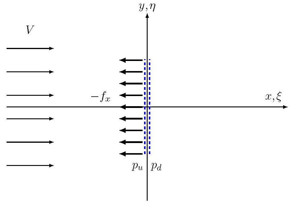
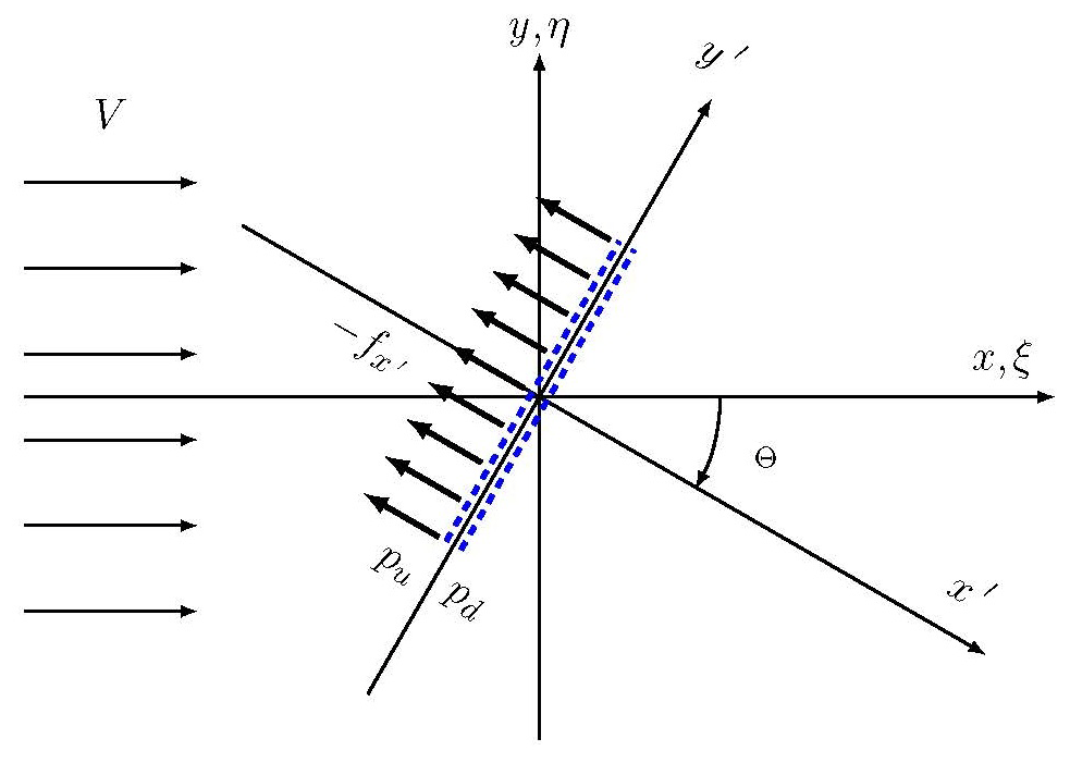
In the linear solution the flow field is only acted upon by the body forces f on the infinitely thin actuator disc as the induced body forces g are assumed to be zero (see Fig. 1 for notation). The pressure field is then derived from Eq. (15), which now has the following form:

$$\begin{array}{}\text{(19)}& {\displaystyle \frac{{\partial }^{\mathrm{2}}p}{\partial x^{\mathrm{2}}}}+{\displaystyle \frac{{\partial }^{\mathrm{2}}p}{\partial y^{\mathrm{2}}}}=\mathrm{0}.\end{array}$$

This is the Laplace equation. The pressure p will thus be a potential function outside the disc showing a jump Δp over the disc. Following the derivation by Koning (1935) the potential function for the pressure can be obtained by covering the surface with doublets with strength Δp. The pressure jump Δp is linked to the body forces f_x as

$$\begin{array}{}\text{(20)}& \mathrm{\Delta }p\left(\mathit{\eta }\right)=\underset{S}{\int }\mathrm{d}\mathit{\eta }\underset{\mathit{ϵ}\to \mathrm{0}}{lim}\underset{-\mathit{ϵ}}{\overset{\mathit{ϵ}}{\int }}{f}_x\mathrm{d}\mathit{\xi }.\end{array}$$

As mentioned above Koning (1935) derived the solution for an axis-symmetric disc, but we will derive the pressure potential for a 2-D disc or in fact an actuator strip with a width of 2b and extending from −z to z and with doublets with the intensity Δp distributed over the surface S. For any point not situated on the disc the potential will, according to Koning (1935), be given by

$$\begin{array}{}\text{(21)}& p={\displaystyle \frac{\mathrm{1}}{\mathrm{4}\mathit{\pi }}}\underset{S}{\int }\mathrm{\Delta }p{\displaystyle \frac{\partial }{\partial n}}\left({\displaystyle \frac{\mathrm{1}}{\mathit{\omega }}}\right)\mathrm{d}S,\end{array}$$

where n denotes the positive normal to the disc and ω the distance from any point on the disc to the point A where the potential is calculated. The details of the derivation can be found in Appendix A.

The resulting pressure function has been derived to

$$\begin{array}{}\text{(22)}& p=-{\displaystyle \frac{\mathrm{1}}{\mathrm{2}\mathit{\pi }}}\underset{-\mathrm{1}}{\overset{{}^{\mathrm{1}}}{\int }}\mathrm{\Delta }p{\displaystyle \frac{x}{x^{\mathrm{2}}+(y-\mathit{\eta }{)}^{\mathrm{2}}}}\mathrm{d}\mathit{\eta }.\end{array}$$

where x and y have been non-dimensionalized with the half width b of the disc.

The induced axial velocity w_x can now be found by integrating Eq. (11) from −∞ to x:

$$\begin{array}{}\text{(23)}& \begin{array}{rl}{w}_x& =-p+\underset{\mathrm{\infty }}{\overset{x}{\int }}{f}_x\mathrm{d}\mathit{\xi }={\displaystyle \frac{\mathrm{1}}{\mathrm{2}\mathit{\pi }}}\underset{-\mathrm{1}}{\overset{{}^{\mathrm{1}}}{\int }}\mathrm{\Delta }p{\displaystyle \frac{x}{x^{\mathrm{2}}+(y-\mathit{\eta }{)}^{\mathrm{2}}}}\mathrm{d}\mathit{\eta }\\ & +\mathrm{\Delta }p(\text{last term only in the wake},x>\mathrm{0}).\end{array}\end{array}$$

The w_y component is determined through Eq. (12) with f_y=0. It means first differentiating p with respect to y and then integrating $\partial p/\partial y$ from −∞ to x. The derivation found in Appendix B leads to the following equation for w_y:

$$\begin{array}{}\text{(24)}& w_y=\underset{\mathrm{\infty }}{\overset{x}{\int }}{\displaystyle \frac{\partial p}{\partial y}}\mathrm{d}\mathit{\xi }={\displaystyle \frac{\mathrm{1}}{\mathrm{2}\mathit{\pi }}}\underset{-\mathrm{1}}{\overset{{}^{\mathrm{1}}}{\int }}\mathrm{\Delta }p{\displaystyle \frac{y-\mathit{\eta }}{x^{\mathrm{2}}+(y-\mathit{\eta }{)}^{\mathrm{2}}}}\mathrm{d}\mathit{\eta }.\end{array}$$

2.2.1 The 2D_l solution for a constant disc loading

With a constant loading Δp on the disc, the pressure and velocity components can be derived by integrating Eqs. (22), (23) and (24) over the width of the disc. The derivation of the pressure function shown in Appendix C leads to

$$\begin{array}{}\text{(25)}& p=-{\displaystyle \frac{\mathrm{1}}{\mathrm{2}\mathit{\pi }}}\mathrm{\Delta }p\left[\arctan {\displaystyle \frac{(\mathrm{1}-y)}{x}}+\arctan {\displaystyle \frac{(\mathrm{1}+y)}{x}}\right],\end{array}$$

and then inserting the pressure equation into Eq. (23), we get

$$\begin{array}{}\text{(26)}& \begin{array}{rl}& w_x={\displaystyle \frac{\mathrm{1}}{\mathrm{2}\mathit{\pi }}}\mathrm{\Delta }p[\arctan {\displaystyle \frac{(\mathrm{1}-y)}{x}}+\arctan {\displaystyle \frac{(\mathrm{1}+y)}{x}}]+\mathrm{\Delta }p\\ & (\text{last term only in the wake},x>\mathrm{0}).\end{array}\end{array}$$

Likewise the integration of w_y for constant loading, shown in Appendix D, yields

$$\begin{array}{}\text{(27)}& w_y={\displaystyle \frac{\mathrm{\Delta }p}{\mathrm{4}\mathit{\pi }}}\ln \left({\displaystyle \frac{x^{\mathrm{2}}+(y+\mathrm{1}{)}^{\mathrm{2}}}{x^{\mathrm{2}}+(y-\mathrm{1}{)}^{\mathrm{2}}}}\right).\end{array}$$

Finally, according to Eqs. (4) and (5) the v_x and v_y velocity components are derived as

$$\begin{array}{}\text{(28)}& {\displaystyle }{v}_x=\mathrm{1}+w_x,\text{(29)}& {\displaystyle }{v}_y=w_y.\end{array}$$

3 AD flow characteristics

In this section we will study the flow characteristics through the 2-D actuator disc by numerical exploration based on the analytical linear solution, 2D_l, for a constant, uniform loading of the disc.

First we relate the pressure jump, Δp, to the thrust, T, and thrust coefficient, C_T:

$$\begin{array}{}\text{(30)}& T=\mathrm{2}b\mathrm{\Delta }p,\end{array}$$

where 2b is the width of the actuator disc.

From the definition of the thrust coefficient, C_T, we get

$$\begin{array}{}\text{(31)}& C_{\mathrm{T}}={\displaystyle \frac{T}{\mathrm{2}b\frac{\mathrm{1}}{\mathrm{2}}\mathit{\rho }{V}^{\mathrm{2}}}}.\end{array}$$

Combining Eqs. (30) and (31) and keeping in mind that Δp is non-dimensionalized with ρV², we get

$$\begin{array}{}\text{(32)}& C_{\mathrm{T}}=\mathrm{2}\mathrm{\Delta }p.\end{array}$$

3.1 Velocity profiles v_x and v_y

For a loading corresponding to a thrust coefficient C_T=0.4 the v_x and v_y velocity profiles as a function of y are shown for different upstream and downstream positions in Fig. 2. The v_x velocity profiles are seen to develop from a Gaussian-type profile upstream of the disc, to be sharper when approaching the disc, and finally at the disc to be completely rectangular with free-stream velocity just outside the disc. Accelerated flow above free-stream velocity is then seen to occur just downstream of the disc and peaking before x=2. Further downstream in the wake the velocity profiles become almost rectangular at x=10 and with a deficit within the projected area of the disc, which means a non-expanding wake.

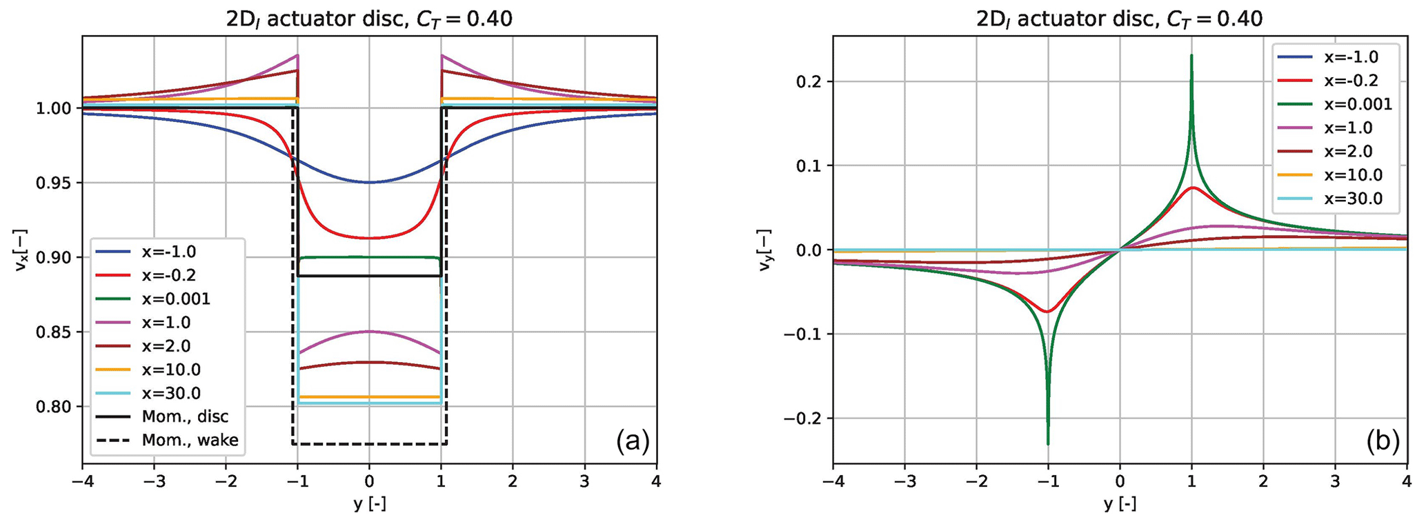
Figure 2 (a) The axial velocity component v_x is shown as a function of the lateral coordinate y for different streamwise positions x from upstream of the disc to far downstream in the wake for a thrust coefficient of 0.4. The velocity profiles for the momentum solution are also shown at the disc and in the far wake. (b) The lateral velocity component v_y is shown for the same positions.

The v_y profiles are seen to be anti-symmetric around the x axis as expected and have a strong peak at the edge of the disc. Downstream the profiles decay fast.

The momentum solution for the v_x component, also shown in Fig. 2, is seen to be lower than the actual linear solution, which will be explored next.

3.2 Scaling C_T to fit the 2D_l solution to momentum theory

As seen above the 2D_l solution does not fit exactly with the classical momentum theory solution for an actuator disc. The computed induction is lower, and it is an important shortcoming for the wider use of the model as a rotor induction model.

To investigate that further we derive the relation between the thrust coefficient C_Tl of the 2D_l model and the induction coefficient, a_l, for the 2D_l solution presented above.

The axial velocity v_xd at the disc is derived from Eq. (26) by $x\to -\mathrm{0}$,

$$\begin{array}{}\text{(33)}& w_{xd}={\displaystyle \frac{\mathrm{\Delta }p}{\mathrm{2}\mathit{\pi }}}\left({\displaystyle \frac{\mathit{\pi }}{\mathrm{2}}}+{\displaystyle \frac{\mathit{\pi }}{\mathrm{2}}}\right)={\displaystyle \frac{\mathrm{\Delta }p}{\mathrm{2}}},\end{array}$$

and from the definition of a,

$$\begin{array}{}\text{(34)}& {\displaystyle }{a}_l=\mathrm{1}-v_{xd}=\mathrm{1}-(\mathrm{1}-w_{xd}),\text{(35)}& {\displaystyle }{a}_l=w_{xd}={\displaystyle \frac{\mathrm{\Delta }p}{\mathrm{2}}}={\displaystyle \frac{C_{\mathrm{Tl}}}{\mathrm{4}}},\end{array}$$

or

$$\begin{array}{}\text{(36)}& C_{\mathrm{Tl}}=\mathrm{4}{a}_l.\end{array}$$

The classical momentum theory derived as an axis-symmetric solution for a circular actuator disc gives the following relation between the thrust coefficient, C_Tm, and the induction, a_m (the subscript m denotes momentum theory):

$$\begin{array}{}\text{(37)}& C_{\mathrm{Tm}}=\mathrm{4}{a}_{\mathrm{m}}(\mathrm{1}-a_{\mathrm{m}}).\end{array}$$

Comparing the solution from the two models, the momentum theory gives a velocity at the disc, v_xm=0.887, for a C_T of 0.4, while the 2D_l model gives v_x=0.9 for a similar C_T.

The reduced induction by the 2D_l model is due to the action of the induced body forces defined in Eqs. (9) and (10) that accelerate the flow in the wake region and also through the disc and upstream of the disc through the pressure field from the g forces.

Without a detailed derivation of the g forces, we can conclude that there will be g_x forces along the lines $y=\pm \mathrm{1}$ in the wake region, which is responsible for the acceleration of the flow through the disc, requiring increased external volume forces, f_x (increased C_Tl), in order to correlate with the velocity at the disc from the momentum solution. A check of the x-momentum balance of a control volume around the disc at some distance will show that the balance is only fulfilled if the g forces are considered as external body forces. This has been demonstrated for the AC flow models based on the same solution approach (Madsen, 1982).

The analogy to use a fixed wake vortex model for the same flow problem would be a vortex sheet along the lines $y=\pm \mathrm{1}$. This vortex sheet will require external body forces to be fixed (non-expanding wake) because the flow in the vicinity of the disc is not aligned with the vortex sheet and thus induces forces on the sheet.

In order to force the 2D_l model to give the same induction in the rotor plane and in the far-field wake as the momentum theory, we can simply scale the thrust coefficient based on Eqs. (36) and (37):

$$\begin{array}{}\text{(38)}& {\displaystyle \frac{C_{\mathrm{Tl}}}{C_{\mathrm{Tm}}}}={\displaystyle \frac{\mathrm{4}{a}_l}{\mathrm{4}{a}_{\mathrm{m}}(\mathrm{1}-a_{\mathrm{m}})}},\end{array}$$

and enforcing a_l to be equal to a_m, we get

$$\begin{array}{}\text{(39)}& \begin{array}{rl}{C}_{\mathrm{Tl}}& =C_{{\mathrm{T}}_{\mathrm{m}}}{\displaystyle \frac{\mathrm{4}{a}_m}{\mathrm{4}{a}_{\mathrm{m}}(\mathrm{1}-a_{\mathrm{m}})}}=C_{{\mathrm{T}}_{\mathrm{m}}}{\displaystyle \frac{\mathrm{1}}{\mathrm{1}-a_{\mathrm{m}}}}\\ & =C_{\mathrm{Tm}}{\displaystyle \frac{\mathrm{2}}{\mathrm{1}+\sqrt{\mathrm{1}-C_{{\mathrm{T}}_{\mathrm{m}}}}}}.\end{array}\end{array}$$

(further down we will denote C_Tm as C_T).

For example for a thrust coefficient of 0.89 we shall increase C_Tl to 1.34 to match the momentum solution as shown in the left graph in Fig. 3. As mentioned above this considerable increase in C_T is necessary due to the strong impact of the g forces on the wake flow, which is seen clearly in the right graph in Fig. 3. Here the v_x velocity profiles together with the enclosing streamlines of the disc show that part of the flow passing through the disc and thus de-accelerated due to the f forces at the disc plane is accelerated up to free-stream velocity at a short distance downstream in the wake region. Although the g forces are only acting from the disc plane and downstream along the lines $y=\pm \mathrm{1}$, the pressure field from these forces will also influence the flow upstream of the disc.

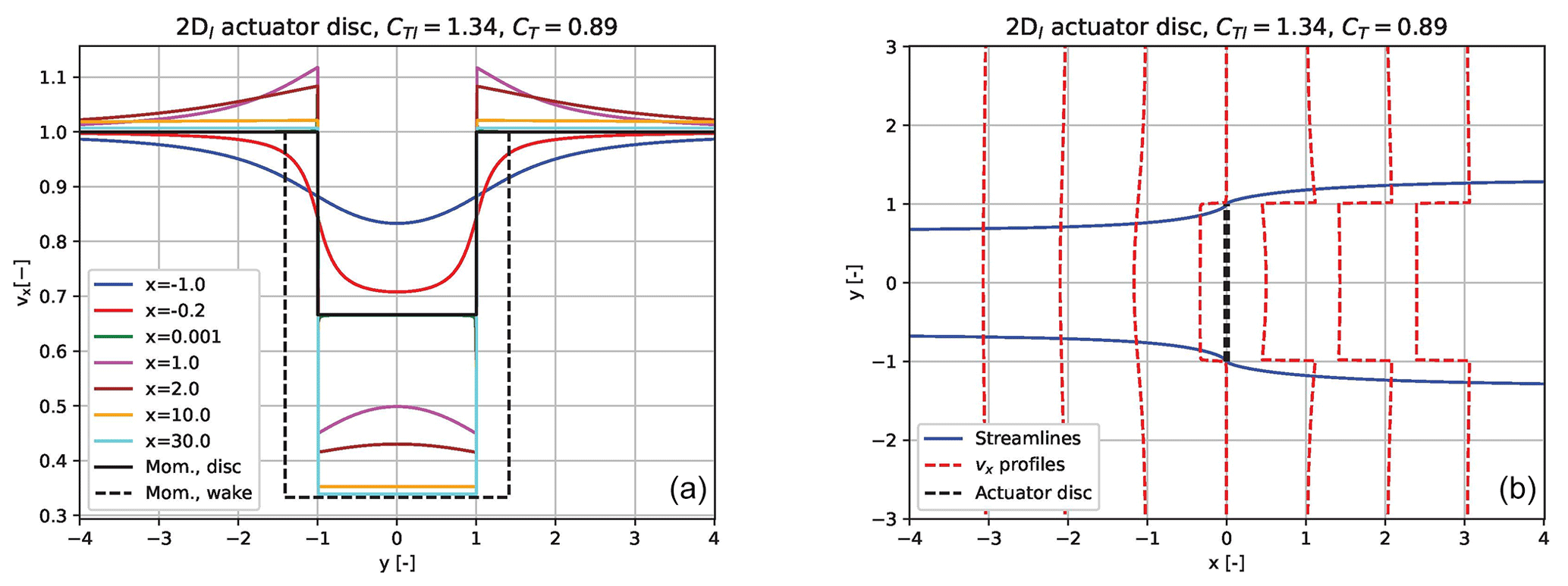
Figure 3 (a) The axial velocity component v_x is shown as a function of the lateral coordinate y for different streamwise positions x from upstream of the disc to far downstream in the wake for a thrust coefficient of 1.34 in the 2D_l model and compared with the momentum solution for a C_T of 0.89. (b) The enclosing streamlines of the disc for the same loading are shown together with v_x profiles at different streamwise positions. The streamlines are derived on the basis of the local flow angle $\arctan \left(\frac{v_y}{v_x}\right)$ with starting points at the edge of the disc.

It can finally be noticed that the same scaling procedure for correcting a linear solution is used in the actuator cylinder model for the VAWT's implemented in HAWC2. However, in this case the correction is applied directly as the scaling of the velocity components (Madsen et al., 2013).

3.3 Superposition of solutions for more discs

As we have a linear model type we can easily study the interaction of more discs with, e.g., different loadings or locations to each other. Later we will show that the superposition is one way to model a coned disc by the superposition of two yawed discs.

Let a new disc 2 have the origin x_D2,y_D2 and a loading Δp_D2 in the original coordinate system as shown in Fig. 1. We then get the contributions v_xD2 and v_yD2 to the velocity field by inserting them into Eqs. (26) and (27):

$$\begin{array}{}\text{(40)}& {\displaystyle }\begin{array}{rl}{w}_{x\mathrm{D}\mathrm{2}}& ={\displaystyle \frac{\mathrm{1}}{\mathrm{2}\mathit{\pi }}}\mathrm{\Delta }{p}_{\mathrm{D}\mathrm{2}}[\arctan {\displaystyle \frac{\mathrm{1}-(y-y_{\mathrm{D}\mathrm{2}})}{x-x_{\mathrm{D}\mathrm{2}}}}\\ & +\arctan {\displaystyle \frac{\mathrm{1}+(y-y_{\mathrm{D}\mathrm{2}})}{x-x_{\mathrm{D}\mathrm{2}}}}]+\mathrm{\Delta }{p}_{\mathrm{D}\mathrm{2}}\\ & \text{(last term only in the wake of disc 2)},\end{array}\text{(41)}& {\displaystyle }{w}_{yD\mathrm{2}}={\displaystyle \frac{\mathrm{\Delta }{p}_{\mathrm{D}\mathrm{2}}}{\mathrm{4}\mathit{\pi }}}\ln \left({\displaystyle \frac{(x-x_{\mathrm{D}\mathrm{2}}{)}^{\mathrm{2}}+((y-y_{\mathrm{D}\mathrm{2}})+\mathrm{1}{)}^{\mathrm{2}}}{(x-x_{\mathrm{D}\mathrm{2}}{)}^{\mathrm{2}}+((y-y_{\mathrm{D}\mathrm{2}})-\mathrm{1}{)}^{\mathrm{2}}}}\right).\end{array}$$

However, the set-up does not work for overlapping discs.

Here the superposition will first be used to study an important characteristic of the model for discs at the same streamwise position with different loadings as in the example in the left part of Fig. 4. The discs are positioned so close that they form one disc with double width, 4b, and with a thrust coefficient of 0.89 and 0.45 on each half. Upstream and downstream of the discs there is a clear interaction between the v_x velocity profiles of the discs, but exactly in the plane of the discs there is no interaction of the axial velocity component, although the thrust coefficient jumps from 0.89 on the lower part to half, 0.445, on the upper part.

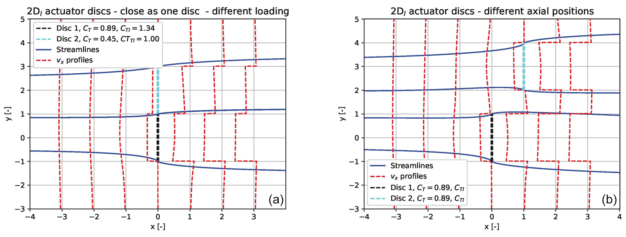
Figure 4 In (a) we show the flow characteristics of two discs placed side by side so they just touch. The lower disc has the double loading of the upper disc. Enclosing streamlines for the two discs are shown together with v_x velocity profiles at different axial positions. (b) The same type of data is shown, however, for the same loading on the two discs and with disc 2 shifted a distance of half the disc width in both x and y directions.

This can be used to guide the implementation of the BEM model in aerodynamic and aeroelastic codes as proposed by Gaunaa et al. (2023) using a VC model for a similar case. The result justifies a local, point-wise evaluation of the momentum balance, e.g., used in the implementation of the BEM model in the HAWC2 code (Madsen et al., 2020). Finally, it should be noticed that there is an interaction of the lateral velocity component in the disc plane.

When the two discs do not have the same streamwise position, we see an interaction of the v_x profiles, as in the case for the example in the right part of Fig. 4. A slightly increased induction can be seen on the upper part of disc 1. Furthermore, an accelerated axial flow velocity between the two discs is noted.

3.4 An important characteristic of the velocity profiles of the 2D_l model at a small distance downstream of the disc and comparison with CFD simulations

In Fig. 3 we saw that at the disc and far downstream in the wake the v_x profiles were rectangular, but in between some bending or curved profiles could be seen, e.g., at x=1 and x=2. We will now go much closer to the disc where we find the development of the profiles as shown in the left graph in Fig. 5. It is clearly seen that the v_x velocity profiles immediately develop from a uniform distribution to shapes with stronger deceleration close to $y=\pm \mathrm{1}$. The same is typically seen in full, non-linear simulations of AD flow (Sørensen and Kock, 1995; Madsen, 1997; Mikkelsen et al., 2001).

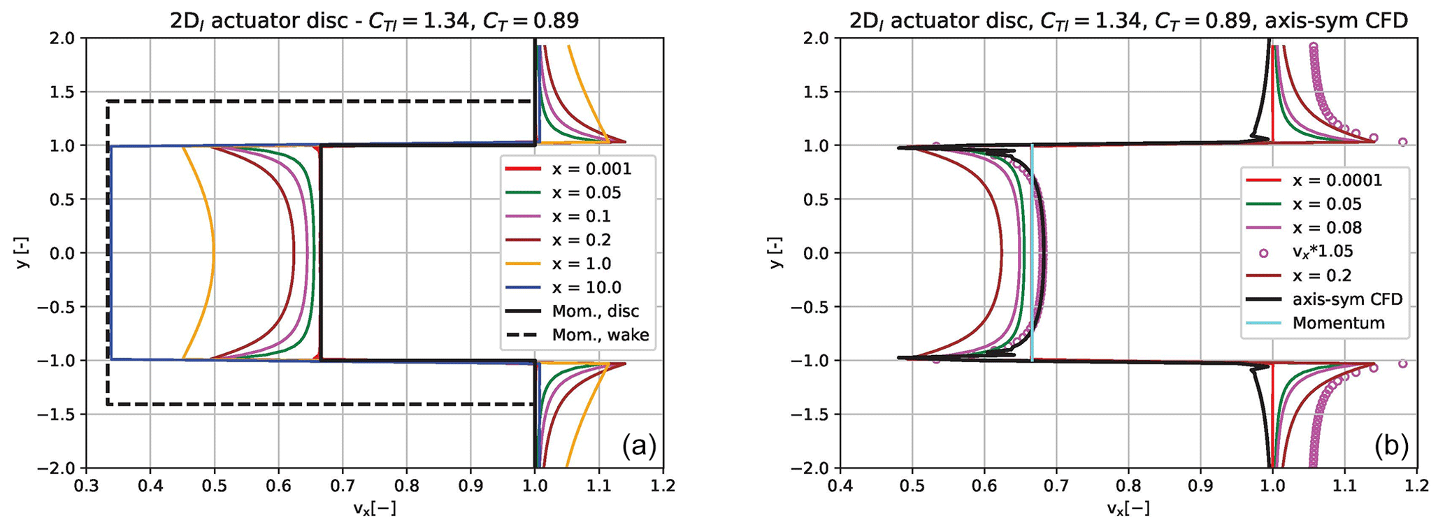
Figure 5 In (a) we show the axial velocity v_x profiles at positions close behind the disc as well as further downstream for a thrust coefficient of 0.89. For comparison the momentum solution for v_x at the disc and in the far wake is also included. (b) The v_x velocity profile at the disc from an axis-symmetric CFD AD simulation is compared with the 2D_l profile at a downstream distance of 0.08 scaled by a factor of 1.05 to account for the decrease in velocity downstream behind the disc and to give the best fit to the CFD results extracted at the disc.

We use here the results of Madsen and Rasmussen (1999) from an axis-symmetric simulation of an AD. Comparing the axial velocity profile at the disc from the CFD simulation with profiles from the 2D_l model extracted at different downstream positions, we find the best correlation in shape using the 2D_l profiles at x=0.08 and scaled by a factor of 1.05, as shown in the right graph of Fig. 5.

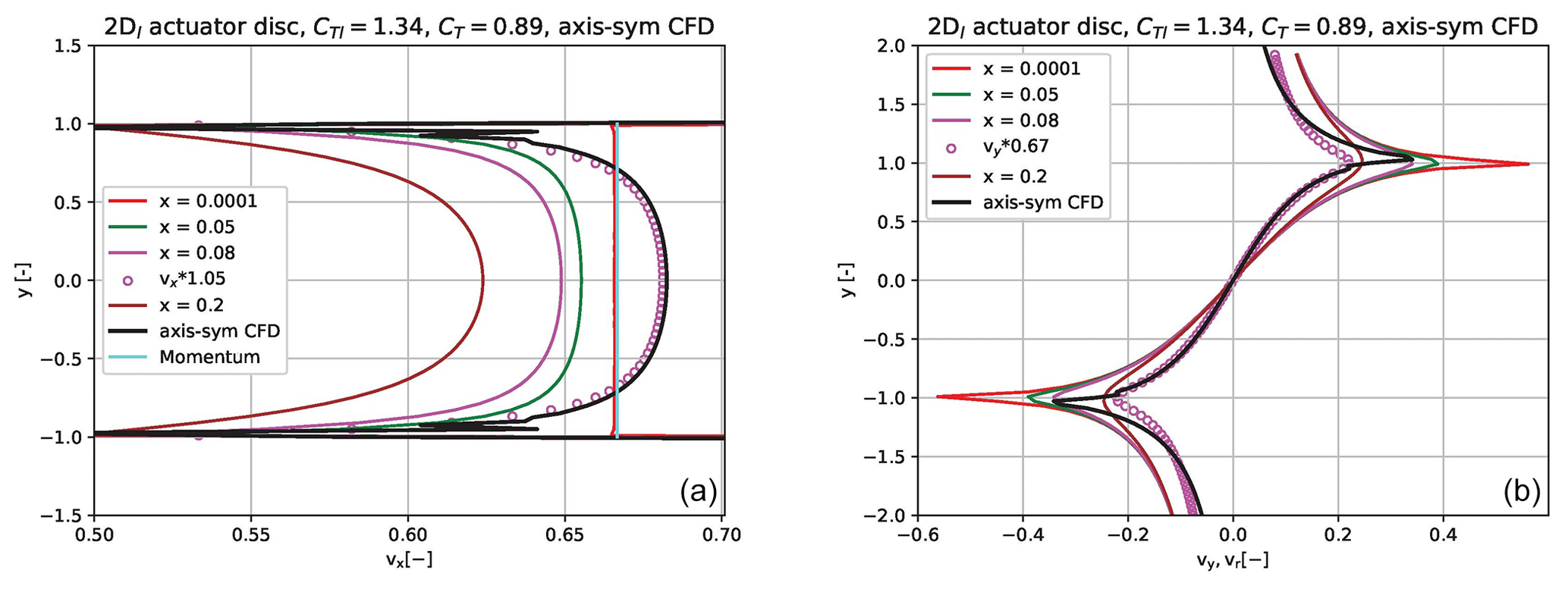
Figure 6 (a) A zoom of the right graph in Fig. 5. (b) 2D_l v_y velocity profiles are compared with the radial velocity profile from an axis-symmetric simulation. At the same downstream position x=0.08 as for the v_x component, the best fit for v_y is obtained by a scaling factor of 0.67.

The reason for this development of the v_x profiles close behind the disc is probably that in this region the g forces along the lines $y=\pm \mathrm{1}$ are acting both upstream and downstream of the axial position where we extract the velocity profiles. Therefore, there might be some local cancelling of their influence so that the deficit is closer to the full solution. The left graph of Fig. 6 shows a very good correlation with the CFD solution when applying the above scaling. It is expected that such scaling is necessary as we have computed the velocity profile a short distance downstream of the disc where the axial velocity decays rapidly. For a wider application of the 2D_l model it is important that the scaling factor is constant. Therefore, we will use the same scaling in the remaining flow examples in the paper.

Finally, the v_y profiles are compared with the profiles of the radial velocity component, v_r, from CFD simulations in the right graph of Fig. 6. When v_y is computed at the same position, x=0.08, as for v_x the best fit is obtained by scaling down by a factor of 0.67. The need for a strong down-scaling is expected as a 2-D solution will have a much stronger lateral velocity component than the radial velocity in an axis-symmetric solution.

4 The 2D_l solution for yawed flow and comparisons with 3-D CFD AD computations with constant loading

We continue now to derive the analytical solution for a 2-D AD in yawed flow (see Fig. 7). This is an important flow situation for a turbine which causes increased loading and reduced power. However, yaw is now frequently studied and used for wake steering in wind farms to increase the power of downstream turbines by upstream wake deflection.

Figure 7 Notation for the 2-D actuator disc in yaw.

The objective with the present model derivation is the further study of the capability of the simple model to handle complex flow like a yawed AD. A further objective is, as the next step (next section), to combine two yawed discs with opposite yaw angles to model a coned rotor.

The starting point is the flow solution for w_x and w_y in Eqs. (26) and (27) in the non-yawed x,y coordinate system which then is rotated by the yaw angle, Θ, into the new system, $x^{\prime },y^{\prime }$ (see Fig. 7). The velocity components, w_x and w_y, in the original system, x,y, are then derived as a function of $x^{\prime },y^{\prime }$.

The following coordinate transformation is introduced:

$$\begin{array}{}\text{(42)}& {\displaystyle }{x}^{\prime }=(x\cos \mathrm{\Theta }-y\sin \mathrm{\Theta }),\text{(43)}& {\displaystyle }{y}^{\prime }=(x\sin \mathrm{\Theta }+y\cos \mathrm{\Theta }).\end{array}$$

The coordinate transformations are inserted into Eqs. (26) and (27):

$$\begin{array}{}\text{(44)}& \begin{array}{rl}{w}_x& ={\displaystyle \frac{\mathrm{\Delta }p}{\mathrm{2}\mathit{\pi }}}\left(\arctan {\displaystyle \frac{\mathrm{1}-(x\sin \mathrm{\Theta }+y\cos \mathrm{\Theta })}{x\cos \mathrm{\Theta }-y\sin \mathrm{\Theta }}}\right.\\ & \left.+\arctan {\displaystyle \frac{\mathrm{1}+(x\sin \mathrm{\Theta }+y\cos \mathrm{\Theta })}{x\cos \mathrm{\Theta }-y\sin \mathrm{\Theta }}}\right),\end{array}\end{array}$$

and

$$\begin{array}{}\text{(45)}& w_y={\displaystyle \frac{\mathrm{\Delta }p}{\mathrm{4}\mathit{\pi }}}\ln \left({\displaystyle \frac{\begin{array}{c}(x\cos \mathrm{\Theta }-y\sin \mathrm{\Theta }{)}^{\mathrm{2}}+\\ \left(\right(x\sin \mathrm{\Theta }+y\cos \mathrm{\Theta })+\mathrm{1}{)}^{\mathrm{2}}\end{array}}{\begin{array}{c}(x\cos \mathrm{\Theta }-y\sin \mathrm{\Theta }{)}^{\mathrm{2}}+\\ \left(\right(x\sin \mathrm{\Theta }+y\cos \mathrm{\Theta })-\mathrm{1}{)}^{\mathrm{2}}\end{array}}}\right).\end{array}$$

The total velocity components, v_x and v_y, for the yawed disc in the x,y coordinate system are then derived as

$$\begin{array}{}\text{(46)}& \begin{array}{rl}& v_x=\mathrm{1}+w_x-\mathrm{\Delta }p(\text{last term only in the wake of the}\\ & \text{yawed disc:}{x}^{\prime }>\mathrm{0}\mathrm{and}y>-\cos \mathrm{\Theta }\mathrm{and}y<\cos \mathrm{\Theta }),\\ & v_y=w_y.\end{array}\end{array}$$

4.1 Streamlines and velocity profiles for a yawed disc of 30, 45 and 60^∘ in comparison with 3-D CFD computations

We will now explore the flow field of a yawed disc of 30, 45 and 60^∘ by presenting enclosing stream lines of the disc and axial velocity profiles from upstream to downstream positions (left graph in Figs. 8, 9 and 10). Further, a comparison with 3-D CFD AD simulations by Madsen (2001) and Madsen et al. (2020) is shown in the graphs to the right.

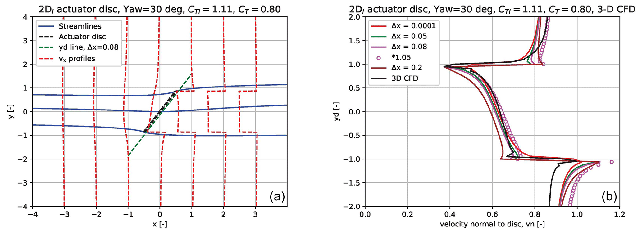
Figure 8 (a) The enclosing streamlines of the yawed disc plus the streamline through the centre of the disc for a yaw of 30^∘. Further, v_x profiles are shown at three x positions. We show also the line yd along the disc at a distance of Δx=0.08, which is the line along which the normal velocity to the disc is shown in (b) in comparison with 3-D CFD simulation of the AD.

Figure 9 Similar graphs as in Fig. 8 above but for a yaw of 45^∘.

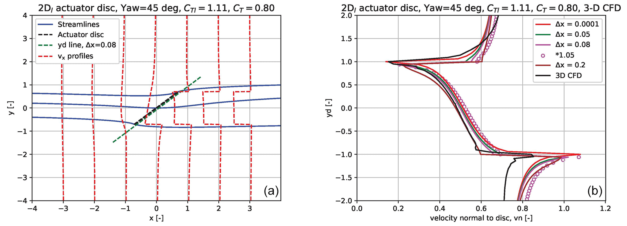
We compare the normal velocity to the disc v_n along a line yd at a distance of Δx=0.08 (see the streamline plots where the yd line is included), which was the distance we found above to give the best correlation with CFD for aligned flow. The normal velocity v_n to the disc is important as it is the velocity component in a rotor simulation with a major influence on the angle of attack (AoA).

We also show v_n along other lines parallel to the disc at other distances Δx, where one is at the disc and one is downstream at Δx=0.2. This is to illustrate the variation in the velocity profiles close behind the disc.

Starting with the evaluation of the results for the yaw case of 30^∘ in Fig. 8 we find overall a very good correlation for the v_n profiles with considerable higher induction on the downstream edge of the disc. Also the non-linear shape in this region fits well with the CFD results. Similar non-linear velocity profiles are seen in the CFD simulations by Troldborg et al. (2014) and by the skewed cylindrical vortex wake model by Branlard and Gaunaa (2015).

Typically in engineering yaw modelling in aerodynamic and aeroelastic codes this velocity distribution is approximated with a linear correlation using the Glauert (1935) model as, e.g., in the implementation of the HAWC2 code (Madsen et al., 2020). We further notice the acceleration of v_n on the upstream edge of the disc and outside, which is stronger than in the CFD results. This can mainly be ascribed to the difference between a 2-D and 3-D flow solution with higher lateral velocities in the 2-D flow.

Continuing with the 45^∘ yaw case in Fig. 9 there is still overall a good correlation between the 2D_l model results and the CFD computations. As above the correlation is almost perfect on the downstream half of the disc, whereas the deviations now are slightly increased on the other half where the 2D_l model computes less induction than the CFD results. Again this is probably due to the 2-D modelling of the flow that results in a stronger acceleration of the lateral flow, in particular outside the disc but now also influencing part of the flow through the disc close to the edge of the disc.

Finally in the 60^∘ yaw case in Fig. 10 we now see major deviations, although the slope of the v_n curves is comparable. Overall the 2D_l model computes less induction over the whole disc, and this might be due to the scaling of C_T based on aligned flow where the wake with the g forces now is offset considerably from one side of the disc to the other.

Figure 10 Similar graphs as in Fig. 8 above but for a yaw of 60^∘.

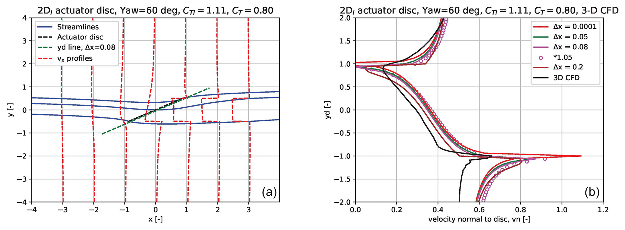
Based on the above comparison cases with 3-D CFD results we can conclude that the 2D_l model simulates yawed flow cases up to 30–40^∘ with quite good accuracy and includes details, like the bending of the v_n curves, not modelled by common engineering yaw models.

5 Modelling of coned rotors with the 2D_l model

Modelling of coned rotors has been of great importance for decades in the wind research community as turbine concept studies often have included downwind coned rotors. This is due to potential advantages by such concepts by alleviating the flapwise blade root moment due to the deloading by centrifugal forces on a coned rotor or blade. In fact the CFD computations on coned rotors (Madsen and Rasmussen, 1999), to be used here for comparisons, were carried out historically to provide input for the design of a small two-bladed rotor (Vølund and Rasmussen, 1999) that could be coned up to 90^∘ for surviving storm situations.

Recent concept studies that include downwind coned rotors are, e.g., Bortolotti et al. (2019), Pao et al. (2021) and Bortolotti et al. (2022). These studies still rely on BEM-type simulation tools which do not model any impact on induction from the coning, which is in contrast to results with higher-fidelity models like the CFD AD simulations presented here.

5.1 Modelling a coned disc by superposition of two yawed discs

The modelling of the coned rotor is based on the superposition of two yawed discs with an opposite yaw angle of ±30^∘, as in the example shown in the left graph of Fig. 11. In this case there is still a distance between the edges of the discs, and we can notice an accelerated flow between the discs.

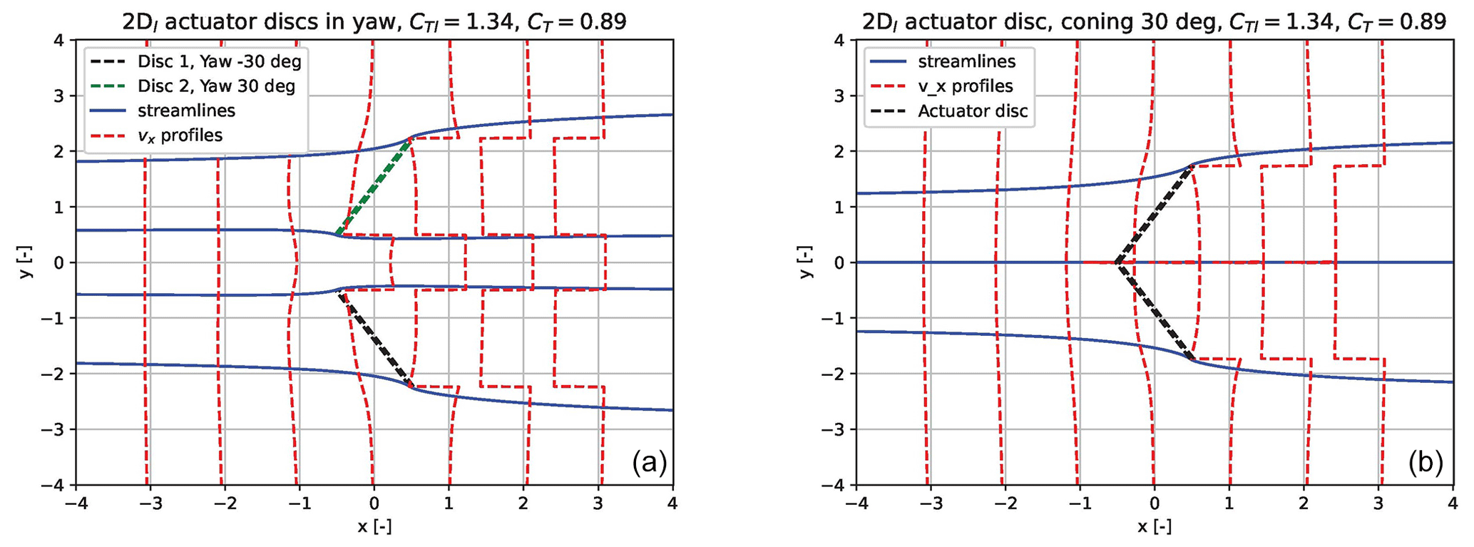
Figure 11 In (a) we show two separated actuator discs with a yaw angle of 30 and −30^∘. In (b) they are moved towards each other so the edges just coincide and form one coned disc of 30^∘ coning.

However, when we now move the discs so close that the two edges just coincide, as shown in the right graph of Fig. 11, we see one velocity deficit behind the two yawed discs and we can call it one coned disc with a cone angle of 30^∘ and the double size of the two yawed discs.

5.2 Comparison of the 2D_l model with an axis-symmetric CFD simulation for a coned disc of 20 and −20^∘

Next we compare the 2D_l solution for a coned rotor with axis-symmetric CFD simulations, as shown in the right graph of Fig. 12. As for the yawed disc we compare v_n as this is the most important velocity component in a rotor simulation with direct influence on angle of attack.

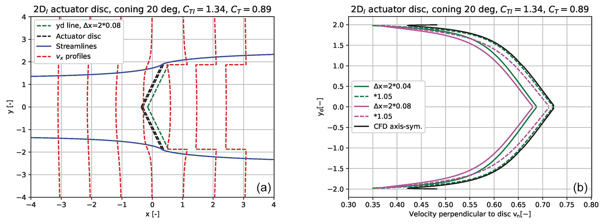
Figure 12 In (a) we show the enclosing streamlines of a coned disc with 20^∘ coning and a C_T=0.89. In the same graph we also show the yd lines parallel with the two disc parts at a distance of $\mathrm{\Delta }x=\mathrm{2}\times \mathrm{0.08}$, which are the lines along which we extract the velocities in the 2D_l model for comparison with the CFD results in (b). However, the CFD velocities were extracted at the disc.

To be consistent with the distance behind the disc where we extract the 2D_l velocities, as tuned for aligned flow, we use the same relative distance behind the disc, which means a double absolute distance $\mathrm{\Delta }x=\mathrm{2}\cdot \mathrm{0.08}$ as the coned disc has double the size of the aligned and yawed disc.

Comparing now the 2D_l simulations with the CFD results we see a very close correlation and just a small underestimation of v_n when using the data extracted at $\mathrm{\Delta }x=\mathrm{2}\cdot \mathrm{0.08}$. An almost complete coincidence is seen for the data extracted slightly closer to the disc at $\mathrm{\Delta }x=\mathrm{2}\cdot \mathrm{0.04}$.

In Fig. 13 we compare next the 2D_l simulations with CFD results for a cone angle of −20^∘. First of all we notice that the shape of the curves are quite different from the velocity profiles for downwind coning as shown above as there is a decrease in the velocity close to the edge. However, the 2D_l model predicts this quite well. The difference occurs when we apply the scaling of the velocities as it shifts the profile slightly towards higher velocities than the CFD results show.

Figure 13 Same type of data as in Fig. 12 but for a cone angle of −20^∘.

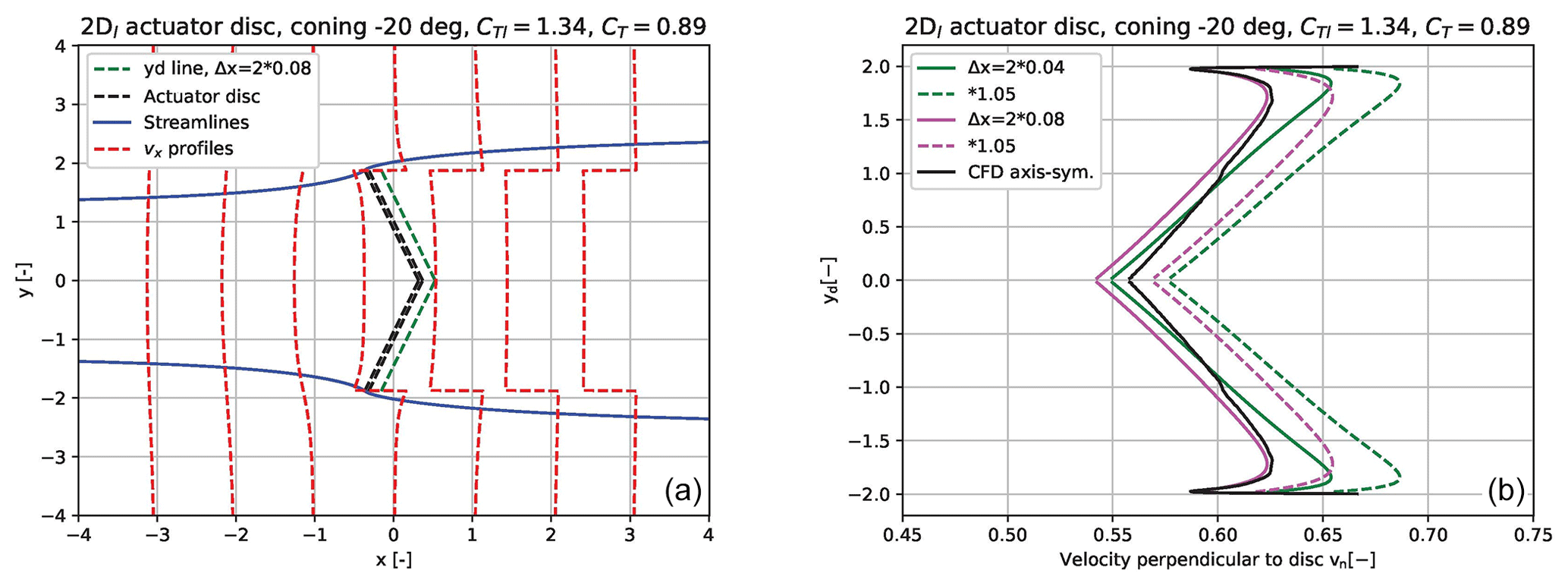
5.3 On the complexity of the flow solution for a coned disc

As mentioned in the Introduction (Sect. 1), Crawford (2006) has proposed a correction to BEM for improving the modelling of a coned rotor. To illustrate with the present model how complex the induction is in a coned disc and thus how challenging a single-point correction of BEM like the one of Crawford (2006) can be, we show in Fig. 14 the v_x and v_y contributions from both sides of the coned disc which then sum up to the total component. Disc 1 is the lower part of the downwind coned rotor, and in the left graph in Fig. 14 the green line is thus the v_x induction from disc 1 itself, whereas the red line is the contribution from the other half, disc 2 of the coned rotor. This contribution is seen to be accelerated flow towards the centre of the coned disc. Likewise we show the same for the v_y component in the graph to the right in Fig. 14. It is seen that the total component is about 0.4 at the tip and therefore contributes significantly to v_n. This illustrates the importance of including the radial component for the derivation of the induction in a coned rotor.

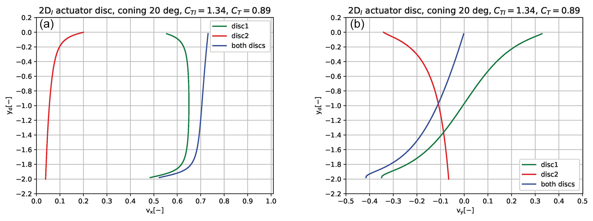
Figure 14 In (a) we show the v_x components contributing to the total induction on the lower part, i.e. disc 1. The same for v_y in (b).

5.4 Flow solution for a range of cone angles

With the 2D_l model we have simulated the normal velocity, v_n, for a range of cone angles from 60 to −60^∘ for a thrust coefficient of 0.89.

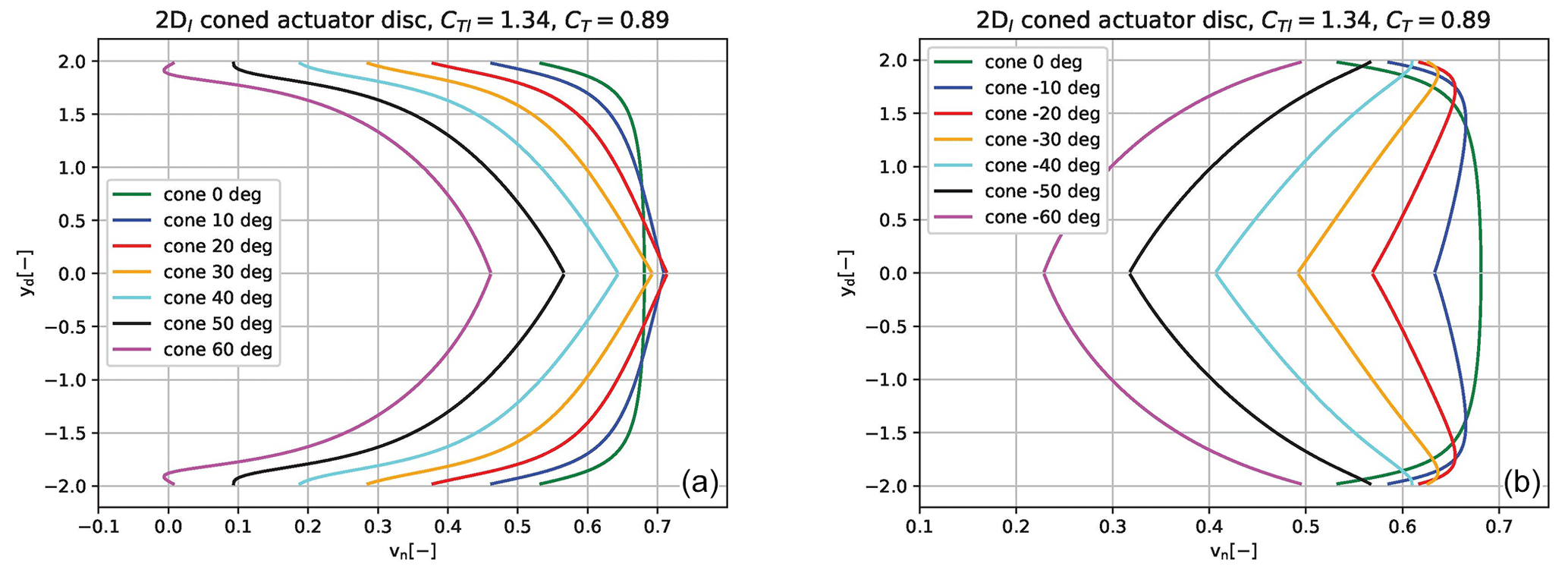
Figure 15 Simulated v_n distributions with the 2D_l model for a range of positive cone angles in (a) and for negative cone angles (b).

In Fig. 15, in the graph to the left with the v_n result for positive cone angles, the shape of the profiles becomes more slender with an increasing difference in velocity at the centre and at the edge. At low cone angles the increase in the normal velocity at the central part of the disc above the velocity for a plane disc can be noticed.

For the negative cone angles in the right graph of Fig. 15 the characteristic sweep on the outer part of the velocity profile towards higher induction can be seen up to a cone angle of about −40^∘.

5.5 Coned disc in yaw

Finally, we have simulated a coned disc of 30^∘ in 20^∘ yawed flow to explore the capability of the 2D_l model to simulate such complex inflow. In the right graph in Fig. 16 we show the enclosing streamlines of the disc. A considerable downward deflection of the wake flow is seen. It means that a bigger part of the flow passing through the lower part of the disc is deflected outside the projected area of the disc and thus accelerated up to the free-stream velocity due to the induced g forces.

In the right graph of Fig. 16 the normal velocity to the disc along the line yd parallel to the disc at a distance of $\mathrm{\Delta }x=\mathrm{2}\times \mathrm{0.08}$ shows as expected a jump passing through the centre of the disc. Further it can be seen that the induction on the two sides of the yawed disc are quite different with a stronger variation from edge to centre on the downwind part.

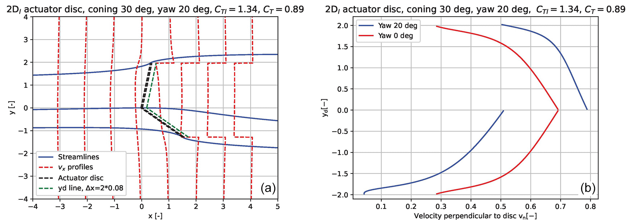
Figure 16 In (a) we show the enclosing streamlines of a 30^∘ coned disc with a yaw angle of 20^∘ together with axial velocity profiles at different streamwise positions. In (b) the normal velocity to the disc along the coned and yawed disc is shown in comparison with the velocities for an aligned coned disc.

6 Outlook

The promising results of the 2D_l model based on comparisons with 3-D and axis-symmetric CFD simulations indicate that although the model is 2-D, it could form the basis for a consistent, general rotor induction model for wind turbine rotors with one equation for v_x and one for v_y including modelling of yawed and coned disc flow. This simplicity would also be of big advantage for the model to be used in rotor optimizations in the derivation of analytical gradients.

One prerequisite for the model to be used for a rotor induction model is a coupling to an angular momentum model for tangential induction. Following the model approach by Madsen et al. (2010) this can be done through the following equation derived from angular momentum balance over the actuator disc combined with a blade element analysis:

$$\begin{array}{}\text{(47)}& v_{\mathrm{t}}={\displaystyle \frac{V_{\mathrm{0}}{C}_Q}{\mathrm{2}(\mathrm{1}-a)}},\end{array}$$

where v_t is the tangential-induced velocity and C_Q is the non-dimensional tangential load coefficient defined as

$$\begin{array}{}\text{(48)}& C_Q={\displaystyle \frac{V_{\mathrm{r}}^{\mathrm{2}}{C}_{x}c{N}_{\mathrm{B}}}{V_{\mathrm{0}}^{\mathrm{2}}\mathrm{2}\mathit{\pi }r}}\end{array}$$

and

$$\begin{array}{}\text{(49)}& C_x=C_l\sin \mathit{\phi }-C_{\mathrm{d}}\cos \mathit{\phi }.\end{array}$$

V_r is the relative velocity to the blade section, c local chord, N_B number of blades, φ the local flow angle from the rotor plane to V_r, C_l and C_d the local airfoil coefficients, and a the axial induction factor which is computed with the 2D_l model.

The specific implementation of the tangential induction model can be discussed, e.g., if it is based on local values or probably best as the average C_Q and a over a ring element.

Likewise the input to the 2D_l model in the form of C_T has to be derived from the blade element analysis and takes a similar form as for C_Q (Madsen et al., 2010):

$$\begin{array}{}\text{(50)}& C_{\mathrm{T}}={\displaystyle \frac{V_{\mathrm{r}}^{\mathrm{2}}{C}_{y}c{N}_{\mathrm{B}}}{V_{\mathrm{0}}^{\mathrm{2}}\mathrm{2}\mathit{\pi }r}},\end{array}$$

with

$$\begin{array}{}\text{(51)}& C_y=C_l\cos \mathit{\phi }+C_{\mathrm{d}}\sin \mathit{\phi }.\end{array}$$

Further on the implementation of the 2D_l model in a rotor analysis, the induction should be computed along diagonal lines of the rotor using the local yaw and tilt angle and cone angle in the 2D_l model. Such an implementation would fit well to the polar grid implementation of BEM in HAWC2 as described in Madsen et al. (2020). The approach could be the computation of the induction along 12–16 diagonals at equally spaced azimuth positions which would give a good resolution of azimuthal variations due to non-uniform inflow and yaw and tilt angles.

It would also be necessary to relax the constant loading assumed for the integration across the disc of Eqs. (23) and (24). However, these integrals can be integrated numerically without slowing down the computations too much or as in the implementation of the actuator cylinder model (Madsen et al., 2013) where the loading is assumed to be piecewise constant which allows the integration of influence coefficients only once in a time simulation.

The capability of the 2D_l model to simulate the flow through a coned rotor in yaw by using two yawed discs of different yaw angles with opposite sign is a big advantage of the model. This allows also for a straightforward simulation of a coned disc in yaw by yawing the one disc more than the other.

The superposition of several differently yawed discs with constant loading could also be used to approximate an arbitrary rotor shape and loading by a segmented diagonal line of discs just coinciding at the edges. This has some resemblance to the approach by Li et al. (2022) where a staggering of VC models shifted in the streamwise direction is used to model non-planar rotors.

A final comment on the 2D_l model is that the evaluation of the velocities at a distance 5 %–10 % behind the disc means that the induction even for a plane rotor is not completely local as there would be velocity contributions from nearby points along the diagonal line. This is considered as an advantage as test cases with high loading in the aeroelastic code HAWC2 (Madsen et al., 2020) using the local induction approach indicate that some averaging of the local C_T should be used.

7 Conclusions

We have presented an analytical linear solution for a 2-D AD flow that is derived from the Euler equations and the equation of continuity. The induction at the disc is uniform for a constant loading like in the momentum theory, but we have shown that immediately behind the disc the axial velocity profiles are non-linear and match by simple scaling a full non-linear axis-symmetric flow solution for an AD.

By a simple coordinate rotation the analytical solution was extended to a yawed disc. This flow solution matches well a full 3-D CFD simulation of a circular AD when comparing the normal velocity to the disc in the plane with skewed inflow up to 30–40^∘.

The superposition of more discs enabled studying turbine interaction and is also used to form a coned disc by positioning two yawed discs with opposite yaw angles so the edges of the discs just coincide. An excellent agreement for a downwind coned disc of 20^∘ was found when comparing the normal velocity to the disc with an axis-symmetric CFD simulation of a coned circular disc. For a disc with upwind coning of −20^∘ the typical shape of the velocity profile with increased induction on the most outboard part matched well the CFD simulations, but some offset of the velocity profile was found.

The promising results of comparing the 2D_l model with 3-D and axis-symmetric CFD simulations on a circular AD have indicated that the 2D_l model could form the basis for a consistent, simple induction model for aerodynamic and aeroelastic wind turbine rotor simulations. First of all the model should for such an application be combined with an angular momentum model which has been sketched in the paper. Then the computation of induction should be used along diagonal lines of the rotor in 12–16 different azimuth positions where the skewed inflow angle from yaw error or tilt is input to the model. Finally, an extension of the present implementation to simulate a variable loading across the disc could be done by numerical integration of the equations for v_x and v_y or by superposition of several yawed discs, each with a constant loading and yaw angle forming a segmented line approximating the real diagonal line of the rotor shape.

Appendix A: Derivation of the pressure function

We show here the derivation of pressure potential for a 2-D disc or in fact an actuator strip extending from −z to z and with doublets with the intensity Δp distributed over the surface S. For any point not situated on the disc the potential will according to Koning (1935) be given by

$$\begin{array}{}\text{(A1)}& p={\displaystyle \frac{\mathrm{1}}{\mathrm{4}\mathit{\pi }}}\underset{S}{\int }\mathrm{\Delta }p{\displaystyle \frac{\partial }{\partial n}}\left({\displaystyle \frac{\mathrm{1}}{\mathit{\omega }}}\right)\mathrm{d}S,\end{array}$$

where n denotes the positive normal to the disc and ω the distance from any point on the disc to the point A where the potential is calculated. ω will then be

$$\begin{array}{}\text{(A2)}& \mathit{\omega }=\sqrt{x^{\mathrm{2}}+(y-\mathit{\eta }{)}^{\mathrm{2}}+{\mathit{\zeta }}^{\mathrm{2}}},\end{array}$$

and inserting into Eq. (21), we get

$$\begin{array}{}\text{(A3)}& \begin{array}{rl}p& ={\displaystyle \frac{\mathrm{1}}{\mathrm{4}\mathit{\pi }}}\underset{-b}{\overset{{}^b}{\int }}\mathrm{\Delta }p\mathrm{d}\mathit{\eta }\underset{-\mathrm{\infty }}{\overset{\mathrm{\infty }}{\int }}{\displaystyle \frac{\partial }{\partial x}}\left({\displaystyle \frac{\mathrm{1}}{\sqrt{x^{\mathrm{2}}+(y-\mathit{\eta }{)}^{\mathrm{2}}+{\mathit{\zeta }}^{\mathrm{2}}}}}\right)\mathrm{d}\mathit{\zeta }\\ & ={\displaystyle \frac{\mathrm{1}}{\mathrm{4}\mathit{\pi }}}\underset{-b}{\overset{{}^b}{\int }}\mathrm{\Delta }p\mathrm{d}\mathit{\eta }\underset{-\mathrm{\infty }}{\overset{\mathrm{\infty }}{\int }}{\displaystyle \frac{-\mathrm{0.5}\cdot \mathrm{2}x}{(x^{\mathrm{2}}+(y-\mathit{\eta }{)}^{\mathrm{2}}+{\mathit{\zeta }}^{\mathrm{2}}{)}^{\mathrm{3}/\mathrm{2}}}}\mathrm{d}\mathit{\zeta }.\end{array}\end{array}$$

The integral is of the type (207) in the handbook of Rumble (2023):

$$\begin{array}{}\text{(A4)}& \underset{-\mathrm{\infty }}{\overset{\mathrm{\infty }}{\int }}{\displaystyle \frac{\mathrm{d}t}{T\sqrt{T}}}=\left[{\displaystyle \frac{\mathrm{2}(\mathrm{2}ct+b)}{q\sqrt{T}}}{|}_{-\mathrm{\infty }}^{\mathrm{\infty }}\right],\end{array}$$

where $T=a+bt+c{t}^{\mathrm{2}}$ and $q=\mathrm{4}ac-b^{\mathrm{2}}$. Now,

$$\begin{array}{ll}{\displaystyle }& {\displaystyle }a=x^{\mathrm{2}}+(y-\mathit{\eta }{)}^{\mathrm{2}},\\ {\displaystyle }& {\displaystyle }b=\mathrm{0},\\ {\displaystyle }& {\displaystyle }c=\mathrm{1},\\ {\displaystyle }& {\displaystyle }q=\mathrm{4}(x^{\mathrm{2}}+(y-\mathit{\eta }{)}^{\mathrm{2}}\left)\right),\\ {\displaystyle }& {\displaystyle }T=x^{\mathrm{2}}+(y-\mathit{\eta }{)}^{\mathrm{2}}+t^{\mathrm{2}}.\end{array}$$

We integrate Eq. (A3):

$$\begin{array}{}\text{(A5)}& {\displaystyle }p=-{\displaystyle \frac{\mathrm{1}}{\mathrm{4}\mathit{\pi }}}\underset{-b}{\overset{{}^b}{\int }}\mathrm{\Delta }p\mathrm{d}\mathit{\eta }\left[x{\displaystyle \frac{\mathrm{2}(\mathrm{2}ct+b)}{q\sqrt{T}}}{|}_{-\mathrm{\infty }}^{\mathrm{\infty }}\right],\text{(A6)}& {\displaystyle }p=-{\displaystyle \frac{\mathrm{1}}{\mathrm{4}\mathit{\pi }}}\underset{-b}{\overset{{}^b}{\int }}\mathrm{\Delta }p\mathrm{d}\mathit{\eta }\left[x{\displaystyle \frac{\mathrm{4}t}{\begin{array}{c}\mathrm{4}[x^{\mathrm{2}}+(y-\mathit{\eta }{)}^{\mathrm{2}}]\\ \sqrt{(x-\mathit{\xi }{)}^{\mathrm{2}}+(y-\mathit{\eta }{)}^{\mathrm{2}}+t^{\mathrm{2}}}\end{array}}}{|}_{-\mathrm{\infty }}^{\mathrm{\infty }}\right],\text{(A7)}& {\displaystyle }\begin{array}{rl}p=& -{\displaystyle \frac{\mathrm{1}}{\mathrm{4}\mathit{\pi }}}\underset{-b}{\overset{{}^b}{\int }}\mathrm{\Delta }p\mathrm{d}\mathit{\eta }[{\displaystyle \frac{x}{[x^{\mathrm{2}}+(y-\mathit{\eta }{)}^{\mathrm{2}}]}}\\ & +{\displaystyle \frac{x}{\left[\right(x-\mathit{\xi }{)}^{\mathrm{2}}+(y-\mathit{\eta }{)}^{\mathrm{2}}]}}],\end{array}\text{(A8)}& {\displaystyle }p=-{\displaystyle \frac{\mathrm{1}}{\mathrm{2}\mathit{\pi }}}\underset{-b}{\overset{{}^b}{\int }}\mathrm{\Delta }p{\displaystyle \frac{x}{x^{\mathrm{2}}+(y-\mathit{\eta }{)}^{\mathrm{2}}}}\mathrm{d}\mathit{\eta }.\end{array}$$

Appendix B: Derivation of the velocity component w_y

The starting point is Eq. (12) with the volume forces $f_y,g_y=\mathrm{0}$:

$$\begin{array}{}\text{(B1)}& {\displaystyle \frac{\partial w_y}{\partial x}}=-{\displaystyle \frac{\partial p}{\partial y}}\end{array}$$

and thus

$$\begin{array}{}\text{(B2)}& w_y=\underset{-\mathrm{\infty }}{\overset{x}{\int }}{\displaystyle \frac{\partial w_y}{\partial x}}\mathrm{d}x=-\underset{-\mathrm{\infty }}{\overset{x}{\int }}{\displaystyle \frac{\partial p_y}{\partial y}}\mathrm{d}x.\end{array}$$

We differentiate the pressure Eq. (A8) with respect to y:

$$\begin{array}{}\text{(B3)}& {\displaystyle \frac{\partial p}{\partial y}}=-{\displaystyle \frac{\mathrm{1}}{\mathrm{2}\mathit{\pi }}}\underset{-\mathrm{1}}{\overset{{}^{\mathrm{1}}}{\int }}\mathrm{\Delta }p{\displaystyle \frac{-\mathrm{2}(y-\mathit{\eta })x}{x^{\mathrm{2}}+(y-\mathit{\eta }{)}^{\mathrm{2}}}}\mathrm{d}\mathit{\eta }.\end{array}$$

Inserting Eq. (B3) into Eq. (B2) gives

$$\begin{array}{}\text{(B4)}& w_y={\displaystyle \frac{\mathrm{1}}{\mathrm{2}\mathit{\pi }}}\underset{-\mathrm{1}}{\overset{{}^{\mathrm{1}}}{\int }}\mathrm{2}(y-\mathit{\eta })\mathrm{\Delta }p\mathrm{d}\mathit{\eta }\underset{-\mathrm{\infty }}{\overset{x}{\int }}{\displaystyle \frac{x}{x^{\mathrm{2}}+(y-\mathit{\eta }{)}^{\mathrm{2}}}}\mathrm{d}x.\end{array}$$

For the integration of the last integral in Eq. (B4) we note the integral is of the type (113) in the handbook of Rumble (2023):

$$\begin{array}{}\text{(B5)}& \int {\displaystyle \frac{t}{T}}={\displaystyle \frac{\mathrm{2}a+bt}{qT}}-{\displaystyle \frac{b}{q}}\int {\displaystyle \frac{\mathrm{d}t}{T}},\end{array}$$

where

$${\displaystyle }T=a+bt+c{t}^{\mathrm{2}}.$$

We have

$$\begin{array}{ll}{\displaystyle }& {\displaystyle }T=t^{\mathrm{2}}+(y-\mathit{\eta }{)}^{\mathrm{2}},\\ {\displaystyle }& {\displaystyle }a=(y-\mathit{\eta }{)}^{\mathrm{2}},\\ {\displaystyle }& {\displaystyle }b=\mathrm{0},\\ {\displaystyle }& {\displaystyle }c=\mathrm{1},\\ {\displaystyle }& {\displaystyle }q=\mathrm{4}ac-b^{\mathrm{2}}=\mathrm{4}(y-\mathit{\eta }{)}^{\mathrm{2}},\end{array}$$

$$\begin{array}{}\text{(B6)}& {\displaystyle }\begin{array}{rl}{w}_y& ={\displaystyle \frac{\mathrm{1}}{\mathrm{2}\mathit{\pi }}}\underset{-\mathrm{1}}{\overset{{}^{\mathrm{1}}}{\int }}\mathrm{2}(y-\mathit{\eta })\mathrm{\Delta }p\mathrm{d}\mathit{\eta }\cdot \left[{\displaystyle \frac{\mathrm{2}a)}{qT}}\right]{|}_{-\mathrm{\infty }}^x\\ & ={\displaystyle \frac{\mathrm{1}}{\mathrm{2}\mathit{\pi }}}\underset{-\mathrm{1}}{\overset{{}^{\mathrm{1}}}{\int }}\mathrm{2}(y-\mathit{\eta })\mathrm{\Delta }p\mathrm{d}\mathit{\eta }\\ & \cdot {\displaystyle \frac{\mathrm{2}(y-\mathit{\eta }{)}^{\mathrm{2}}}{\left(\mathrm{4}\right(y-\mathit{\eta }{)}^{\mathrm{2}}\left)\right(x^{\mathrm{2}}+(y-\mathit{\eta }{)}^{\mathrm{2}})}},\end{array}\text{(B7)}& {\displaystyle }{w}_y={\displaystyle \frac{\mathrm{1}}{\mathrm{2}\mathit{\pi }}}\underset{-\mathrm{1}}{\overset{{}^{\mathrm{1}}}{\int }}\mathrm{\Delta }p{\displaystyle \frac{(y-\mathit{\eta })}{(x^{\mathrm{2}}+(y-\mathit{\eta }{)}^{\mathrm{2}})}}\mathrm{d}\mathit{\eta }.\end{array}$$

Appendix C: Derivation of the pressure function for constant loading

The pressure function has in Eq. (A8) been derived to

$$\begin{array}{}\text{(C1)}& p=-{\displaystyle \frac{\mathrm{1}}{\mathrm{2}\mathit{\pi }}}\underset{-\mathrm{1}}{\overset{{}^{\mathrm{1}}}{\int }}\mathrm{\Delta }p{\displaystyle \frac{x}{x^{\mathrm{2}}+(y-\mathit{\eta }{)}^{\mathrm{2}}}}\mathrm{d}\mathit{\eta }.\end{array}$$

When the loading Δp is constant, we can derive the analytical solution for the pressure.

The integral is of the type (107) in the handbook of Rumble (2023):

$$\begin{array}{}\text{(C2)}& \int {\displaystyle \frac{\mathrm{d}t}{T}}={\displaystyle \frac{\mathrm{2}}{\sqrt{q}}}\arctan {\displaystyle \frac{\mathrm{2}ct+b}{\sqrt{q}}},\end{array}$$

where

$${\displaystyle }T=a+bt+c{t}^{\mathrm{2}}.$$

We have

$$\begin{array}{ll}{\displaystyle }& {\displaystyle }T=t^{\mathrm{2}}-\mathrm{2}yt+(x^{\mathrm{2}}+y^{\mathrm{2}}),\\ {\displaystyle }& {\displaystyle }a=x^{\mathrm{2}}+y^{\mathrm{2}},\\ {\displaystyle }& {\displaystyle }b=-\mathrm{2}y,\\ {\displaystyle }& {\displaystyle }c=\mathrm{1},\\ {\displaystyle }& {\displaystyle }q=\mathrm{4}ac-b^{\mathrm{2}}=\mathrm{4}(x^{\mathrm{2}}+y^{\mathrm{2}})-(-\mathrm{2}y{)}^{\mathrm{2}},\\ {\displaystyle }& {\displaystyle }\sqrt{q}=\mathrm{2}x,\end{array}$$

$$\begin{array}{}\text{(C3)}& {\displaystyle }\begin{array}{rl}p& =-{\displaystyle \frac{\mathrm{1}}{\mathrm{2}\mathit{\pi }}}x\mathrm{\Delta }p\left[{\displaystyle \frac{\mathrm{2}}{\mathrm{2}x}}\arctan \right({\displaystyle \frac{\mathrm{2}t-\mathrm{2}y)}{\mathrm{2}x}}\left)\right]{|}_{-\mathrm{1}}^{\mathrm{1}}\\ & =-{\displaystyle \frac{\mathrm{1}}{\mathrm{2}\mathit{\pi }}}x\mathrm{\Delta }p\left[{\displaystyle \frac{\mathrm{2}}{\mathrm{2}x}}\arctan \right({\displaystyle \frac{\mathrm{2}-\mathrm{2}y}{\mathrm{2}x}})\\ & -\arctan \left({\displaystyle \frac{-\mathrm{2}-\mathrm{2}y}{\mathrm{2}x}}\right)],\end{array}\text{(C4)}& {\displaystyle }p=-{\displaystyle \frac{\mathrm{1}}{\mathrm{2}\mathit{\pi }}}\mathrm{\Delta }p\left[\arctan \right({\displaystyle \frac{\mathrm{1}-y}{x}})+\arctan ({\displaystyle \frac{\mathrm{1}+y}{x}}\left)\right].\end{array}$$

Appendix D: Derivation of w_y for a constant loading

w_y has in Eq. (24) been derived to

$$\begin{array}{}\text{(D1)}& w_y={\displaystyle \frac{\mathrm{1}}{\mathrm{2}\mathit{\pi }}}\underset{-\mathrm{1}}{\overset{{}^{\mathrm{1}}}{\int }}\mathrm{\Delta }p{\displaystyle \frac{y-\mathit{\eta }}{x^{\mathrm{2}}+(y-\mathit{\eta }{)}^{\mathrm{2}}}}\mathrm{d}\mathit{\eta }.\end{array}$$

The integrals are of the type (112) in the handbook of Rumble (2023),

$$\begin{array}{}\text{(D2)}& -\int {\displaystyle \frac{\mathrm{d}t\cdot t}{T}}=-{\displaystyle \frac{\mathrm{1}}{\mathrm{2}c}}\ln T+{\displaystyle \frac{b}{\mathrm{2}c}}\int {\displaystyle \frac{\mathrm{d}t}{T}},\end{array}$$

and (107)

$$\begin{array}{}\text{(D3)}& y\int {\displaystyle \frac{\mathrm{d}t}{T}},\end{array}$$

where

$${\displaystyle }T=a+bt+c{t}^{\mathrm{2}}$$

and

$$\begin{array}{ll}{\displaystyle }& {\displaystyle }T=t^{\mathrm{2}}-\mathrm{2}yt+(x^{\mathrm{2}}+y^{\mathrm{2}}),\\ {\displaystyle }& {\displaystyle }a=x^{\mathrm{2}}+y^{\mathrm{2}},\\ {\displaystyle }& {\displaystyle }b=-\mathrm{2}y,\\ {\displaystyle }& {\displaystyle }c=\mathrm{1},\\ {\displaystyle }& {\displaystyle }q=\mathrm{4}ac-b^{\mathrm{2}}=\mathrm{4}(x^{\mathrm{2}}+y^{\mathrm{2}})-(-\mathrm{2}y{)}^{\mathrm{2}}=\mathrm{4}{x}^{\mathrm{2}},\\ {\displaystyle }& {\displaystyle }\sqrt{q}=\mathrm{2}x.\end{array}$$

We first notice that the last integral in Eq. (B6) cancels out the integral in Eq. (D3), as we have

$$\begin{array}{}\text{(D4)}& {\displaystyle \frac{b}{\mathrm{2}c}}\int {\displaystyle \frac{\mathrm{d}t}{T}}={\displaystyle \frac{-\mathrm{2}y}{\mathrm{2}}}\int {\displaystyle \frac{\mathrm{d}t}{T}}=-y\int {\displaystyle \frac{\mathrm{d}t}{T}}.\end{array}$$

For the other integral in Eq. (B6), when inserting into Eq. (D1), we have

$$\begin{array}{}\text{(D5)}& {\displaystyle }{w}_y=-{\displaystyle \frac{\mathrm{1}}{\mathrm{2}\mathit{\pi }}}\mathrm{\Delta }p\left[{\displaystyle \frac{\mathrm{1}}{\mathrm{2}}}\ln \right(t^{\mathrm{2}}-\mathrm{2}yt+(x^{\mathrm{2}}+y^{\mathrm{2}})\left)\right]{|}_{-\mathrm{1}}^{\mathrm{1}}=>,\text{(D6)}& {\displaystyle }\begin{array}{rl}{w}_y& ={\displaystyle \frac{\mathrm{1}}{\mathrm{4}\mathit{\pi }}}\mathrm{\Delta }p\left[\ln \right(\mathrm{1}-\mathrm{2}y+(x^{\mathrm{2}}+y^{\mathrm{2}}))\\ & -\ln (\mathrm{1}+\mathrm{2}y+(x^{\mathrm{2}}+y^{\mathrm{2}}\left)\right)]=>,\end{array}\text{(D7)}& {\displaystyle }{w}_y=-{\displaystyle \frac{\mathrm{1}}{\mathrm{4}\mathit{\pi }}}\mathrm{\Delta }p\left[\ln \right({\displaystyle \frac{x^{\mathrm{2}}+(y+\mathit{\eta }{)}^{\mathrm{2}}}{x^{\mathrm{2}}+(y-\mathit{\eta }{)}^{\mathrm{2}}}}\left)\right].\end{array}$$

Appendix E

Table E1 List of symbols.