the Creative Commons Attribution 4.0 License.
the Creative Commons Attribution 4.0 License.
 | 19 Dec 2023
Feedforward pitch control for a 15 MW wind turbine using a spinner-mounted single-beam lidar
David Schlipf
Alfredo Peña
Feedforward blade pitch control is one of the most promising lidar-assisted control strategies due to its significant improvement in rotor speed regulation and fatigue load reduction. A high-quality preview of the rotor-effective wind speed is a key element of control benefits. In this work, a single-beam lidar is simulated in the spinner of a bottom-fixed IEA 15 MW wind turbine. Both continuous-wave (CW) and pulsed lidar systems are considered. The single-beam lidar can rotate with the wind turbine rotor and scan the inflow with a circular pattern, which mimics a multiple-beam nacelle lidar at a lower cost. Also, the spinner-based lidar has an unimpeded view of the inflow without intermittent blockage from the rotating blade. The focus distance and the cone angle of the spinner-based single-beam lidar are optimized for the best wind preview quality based on a rotor-effective wind speed coherence model. Then, the control benefits of using the optimized spinner-based lidar are evaluated for an above-rated wind speed in OpenFAST with an embedded lidar simulator and virtual four-dimensional Mann turbulence fields considering the wind evolution. Results are compared against those using a single-beam nacelle-based lidar. We found that the optimum scanning configurations of both CW and pulsed spinner-based single-beam lidars lead to a lidar scan radius of 0.6 of the rotor radius. Also, results show that a single-beam lidar mounted in the spinner provides many more control benefits (i.e. better rotor speed regulations and higher reductions in the damage equivalent loads on the tower base and blade roots) than the one based on the nacelle. The spinner-based single-beam lidar has a similar performance to a four-beam nacelle lidar when used for feedforward control.
- Article
(3925 KB) - Full-text XML
- BibTeX
- EndNote


In the past decade, lidar-assisted wind turbine control (LAC) has received growing interest in the wind energy community. Among different control strategies, blade pitch feedforward control is one of the most promising LAC techniques, due to the significant improvement in the regulation of the rotor speed and the reduction in the fatigue loads compared to using conventional feedback controllers alone (Canet et al., 2021). Whereas the feedback controller reacts to the wind disturbance after the effect of turbulent wind on the structure has occurred, the feedforward controller is able to utilize the preview information of the approaching wind provided by, e.g. lidars, which helps the turbine to react in advance. The collective pitch control strategy, in which the blades are all controlled together, uses the rotor-effective wind speed (REWS) as a key input to the feedforward controller.
In 2022, the installed prototype of the world's biggest wind turbine had a rated power of 15 MW. It has reached over 200 m in height, and the rotor-swept area is equivalent to four soccer fields (Venditti, 2022). The inflow to wind turbines of such size cannot be measured by anemometers installed on a meteorological mast. The nacelle-mounted anemometers operate in the wake of the rotor and do not measure the free-stream wind speed. As remote sensing devices, forward-looking lidars mounted on the nacelle or the spinner of the wind turbines have a better sight of the wind approaching the rotor, and they can provide a high-quality wind preview. They are aligned with the wind turbine rotor and always track the incoming wind. Also, nacelle lidars can measure the inflow remotely at different locations over the rotor-swept area. The REWS estimated from a lidar system by combining the radial measurements over a full scan might more closely resemble the true REWS, which is the spatial average of the longitudinal wind velocities across the rotor disc (Schlipf et al., 2015a), than a pointwise anemometer. Therefore, they have the potential to deliver inflow characteristics that are better correlated with turbine signals (rotor speed, fatigue loads, etc.) than those derived from pointwise anemometers, e.g. cup and sonic anemometers.
Two types of nacelle lidar systems have been tested for wind turbine control, namely the continuous-wave (CW) and pulsed systems. The CW lidars usually measure at one focus distance at a time at a high sampling rate. Pulsed lidars are able to collect backscattered signals from several measurement ranges according to the response time, but they require typically long sampling periods. Both lidars have been reported to be useful for LAC (Mikkelsen et al., 2013; Kumar et al., 2015). Schlipf et al. (2014) found a decrease in the rotor speed variation during the above-rated operation of CART2 using feedforward pitch control and a circularly scanning pulsed lidar. Scholbrock et al. (2013) showed the mitigation on tower fore–aft loads using measurements from a three-beam pulsed lidar for the feedforward controller on CART3. Scholbrock et al. (2015) achieved a reduction in yaw error using the circularly scanning CW lidar, replacing the turbine-based wind vane. Although many other relevant studies are based on aero-elastic simulations (Harris et al., 2006a; Bossanyi et al., 2012; Simley et al., 2014), the results from the above experiments demonstrate improvements in wind turbine performance when using LAC (Simley et al., 2018).
The benefit of LAC needs to be balanced with the investment in using nacelle lidars. The simplest option is a single-beam staring lidar system. As the first field test of a nacelle-mounted lidar, Harris et al. (2006b) demonstrated that a single-beam CW lidar measuring at hub height is able to detect the fluctuations in the longitudinal velocity at 200 m upstream of a Nordex N90 wind turbine. Nevertheless, the measurement at a single location is not representative of the REWS.
Compared to the staring lidar mounted on the wind turbine nacelle, the single-beam lidar in the spinner can rotate with the rotor during turbine operation, scan a good portion of the inflow coming to the rotor disc, and reduce the cost of nacelle lidars relying on complex scanning patterns. Another advantage of using a spinner-based lidar, over a nacelle-mounted system, is the unimpeded view of the inflow without intermittent signal blockage by the blades, which increases data availability. A proof-of-concept field experiment was conducted by Mikkelsen et al. (2013), in which a ZephIR single-beam lidar system was deployed in the spinner of an NM80 2.3 MW wind turbine. They showed that the system is capable of measuring the upcoming wind and turbulence structure in real time. Based on a simulation study of the spinner-based CW lidar on the NREL 5 MW wind turbine, Simley et al. (2014) examined the accuracy of different measurement scenarios and found the best along-wind component estimation at a lidar scan radius of 75 % blade span, while the lidar provides the best blade-effective wind speed estimation at 69 % blade span.
This work aims to demonstrate the usefulness of a single-beam lidar for wind turbine feedforward control if the lidar is mounted in the spinner compared to a nacelle-based system. Our reference wind turbine is the bottom-fixed variable-speed collective-pitch-controlled IEA 15 MW turbine (design class 1B) with a rotor diameter of 240 m and a hub height of 150 m (National Renewable Energy Laboratory, 2020). We consider both continuous-wave and pulsed Doppler lidars. Based on the four-dimensional (4D) Mann turbulence model that considers wind evolution (Guo et al., 2022a), we optimize the focus distance and the cone angle of the spinner-mounted single-beam lidar to achieve the highest coherence between the rotor- and the lidar-estimated REWS. Then, through time-domain simulations using the 4D Mann turbulence fields with typical turbulence parameters of near-neutral atmospheric stability conditions, the performance of the feedforward control using the optimized lidar is evaluated. The Reference Open-Source COntroller (ROSCO) controller (Abbas et al., 2022) is used as the reference feedback controller. The simulations are conducted in the open-source aero-elastic tool OpenFAST (National Renewable Energy Laboratory, 2022), and the results are compared against those using a single-beam nacelle-based lidar.
This paper is organized as follows. Section 2 describes the background for this work, including the turbulence spectral model, the modelling of the wind evolution, the spinner-based lidar, and the wind preview quality. Section 3 introduces the set-up of time-domain simulations. Section 4 shows the results of the lidar configuration optimization, which is followed by Section 5, where we evaluate the performance of the feedforward control. Discussion of results is given in Sect. 6. Section 7 concludes the work and provides the outlook.
2.1 Mann turbulence spectral model
The three-dimensional (3D) wind field can be described by a vector field at a given time t0, where u,v, and w are the horizontal along-wind, the horizontal lateral, and the vertical wind components, respectively. The vector is the position vector defined in the righthanded Cartesian coordinate system. Using Reynolds decomposition, the wind field can be decomposed into the mean wind speed , where 〈⋅〉 denotes ensemble averaging and the fluctuating components . Assuming Taylor's frozen hypothesis (Taylor, 1938), the velocity fluctuations do not change with time but propagate in the along-wind direction with a velocity equal to the mean wind speed. Therefore, the wind field after a given time Δt can be derived as
The wind field can also be expressed in the wavenumber domain using the following 3D Fourier transform:
where and . Denoting a complex conjugate by * and the three velocity components by indices , the ensemble average of the Fourier coefficients is the spectral velocity tensor
With the Dirac delta function δ(⋅), Eq. (3) implies the homogeneity in the stochastic wind field; i.e. is 0 for . Here, we assume that the spectral tensor Φij(k) can be described by the Mann model (Mann, 1994), in which, besides the wave number k, three adjustable parameters are used: , where α is the spectral Kolmogorov constant and ε the turbulent energy dissipation rate; L, which is a length scale describing the size of the most energy-containing eddies; and Γ, which represents the turbulence anisotropy and distortion of the eddies from the vertical velocity shear in the atmospheric surface layer. The characteristics of the Mann model permit the modelling of 3D spectra and coherence. The model is recommended by the IEC 61400-1 standard (IEC, 2019) for the calculation of wind turbine loads.
2.2 Temporal evolution of turbulence
Turbulence structures evolve when they approach the rotor. To consider the temporal evolution of turbulence, we assume that the stochastic field travels with the mean wind speed U in the along-wind direction. However, we assume the turbulent eddies decay exponentially with time. The spectral velocity tensor Φij then becomes the space–time tensor Θij (Guo et al., 2022a):
with
where τe is a new eddy lifetime that considers the temporal evolution. We also assume this eddy lifetime as in Guo et al. (2022a):
where γ is a coefficient that determines the strength of turbulence evolution. Guo et al. (2022a, 2023) considered γ≈400 for near-neutral atmospheric stability conditions and γ≈200 for stable atmospheric conditions.
The 1D cross-spectra of all velocity fluctuations with separations Δy and Δz that consider evolution are then the following:
where . The one-point cross-spectra and auto-spectra of the velocity components can be obtained when the separations Δy and Δz are 0, and i=j in Eq. (7). The magnitude-squared coherence of all velocity components is
where
2.3 Spinner-mounted single-beam lidar
In this work, we simulate a single-beam lidar system mounted in the wind turbine spinner. With an angle between the beam and the turbine's horizontal axis, the spinner-based lidar is able to scan the inflow in a circular pattern without signal blockage from the turbine blades or the nacelle, which is otherwise an issue in nacelle-mounted lidars. Figure 1 shows the scanning trajectory of the single-beam lidar in the spinner of the 15 MW turbine, where the x, y, and z axes describe the coordinates of the 3D wind field, as introduced in Sect. 2.1. The mean wind direction is along the x axis. The beam orientation n can be expressed as
where ϕ is the half-cone opening angle, and θ is the angle between the y axis and the beam direction projected on the y–z plane. The beam unit vector can also be expressed with the beam azimuth α and elevation angle β, which is used in the OpenFAST lidar simulator (Guo et al., 2022b):
The rotor shaft of the reference wind turbine has a tilt angle of 6∘. Therefore, the lidar beam unit vector is rotated around the y axis. The red circles in Fig. 1 indicate the scanning locations of the single-beam lidar before the rotation around the y axis.
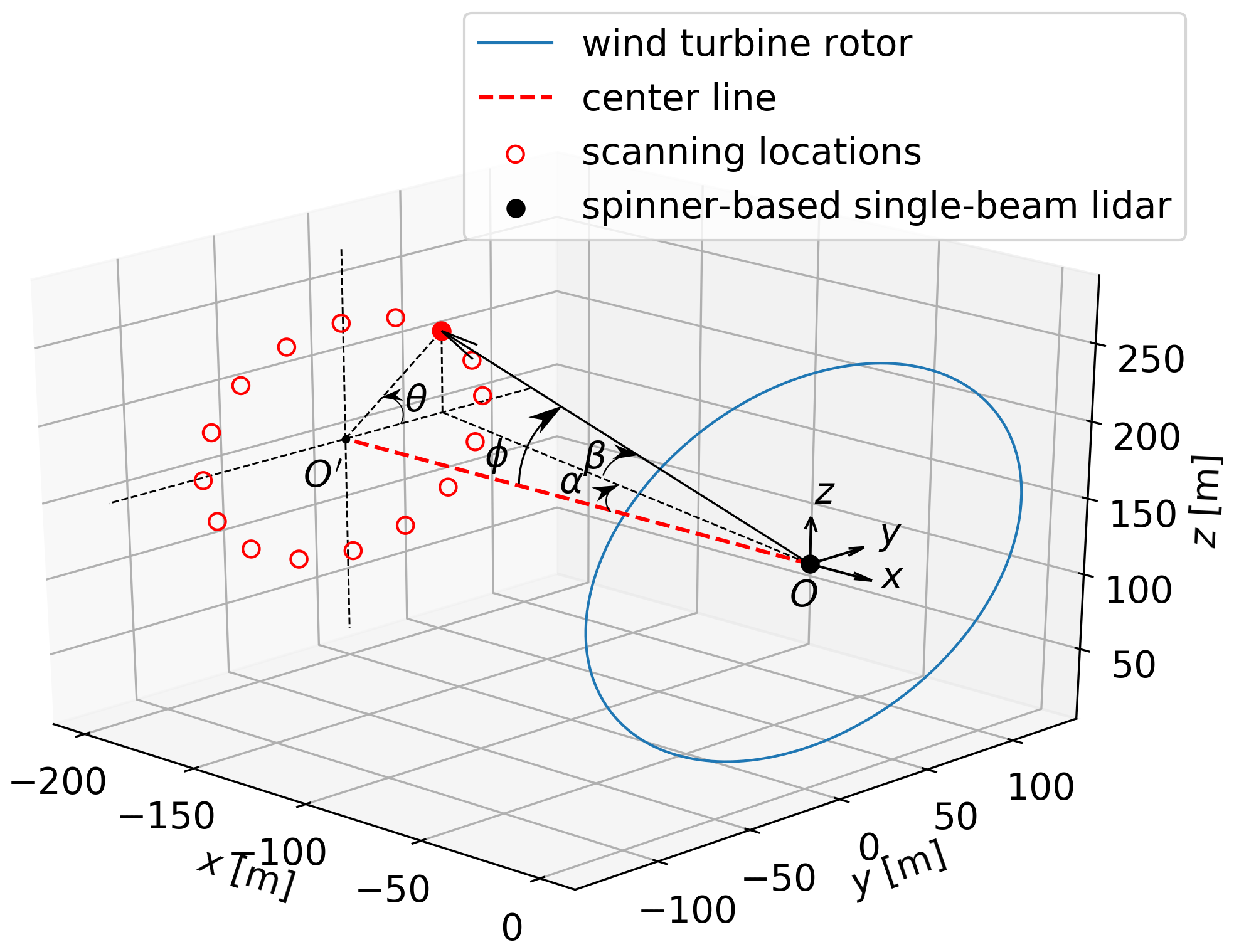
Figure 1Scanning trajectory of the single-beam lidar in the IEA 15 MW wind turbine spinner. The lidar angles used are marked.
Since the typical feedforward collective pitch controller is only active at above-rated wind speeds, the rotational speed of the wind turbine has reached its rated value. For the reference wind turbine, the rated wind speed is vR=10.59 m s−1, and the rated rotor speed is ΩR=7.56 rpm. The turbine is controlled to maintain its rotor speed close to the rated value. Therefore, the single-beam lidar needs around 8 s ( rpm) to complete a full scan. Assuming that the rotor speed is almost constant and the beam scanning locations are fixed with a sampling frequency fs=4 Hz, the spinner-based lidar can measure 32 radial velocities in one circular scan. Therefore, θ can be modelled as
where i=1, 2, …, 32 is the beam index.
Assuming that the dominant radial velocity vr in the Doppler spectrum of radial velocities within the probe volume can be determined by the centroid method (Held and Mann, 2018; Fu et al., 2022), vr is the convolution of the lidar weighting function due to its probe volume φ(s) and the wind components along the beam:
The weighting function of a CW lidar system is approximated by a Lorentzian function as follows (Sonnenschein and Horrigan, 1971):
where s is the distance to the beam focus, and zR is the Rayleigh length determined by the focus distance fd, the laser wavelength λ, and the transmitted beam radius at the exit of the optical lens rb,
The Fourier transformation of Eq. (14) is
For pulsed systems, we assume the weighting function has a Gaussian shape parameterized by a standard deviation σL (Cariou, 2013):
with
where WL is the full-width at half maximum (FWHM). The Fourier transform of Eq. (17) is
It can be seen from Eqs. (15) and (18) that the probe volume of CW lidars increases with the square of the focus distance, whereas it is constant at any range for pulsed systems. In our study, we assume λ=1.565 µm, rb=28 mm, and WL=30 m (Peña et al., 2016).
The weighting functions need to be truncated and discretized to simulate lidar measurements in turbulence boxes of finite length. We discretize Eq. (14) with a resolution of Δs=0.1zR considering smax=6zR and . Similarly, for Eq. (17), we use smax=1.5WL and with a resolution of Δs=2.5 m (around 0.08WL). The discretized weights are normalized to have the sum equal to 1. Since WL=2zR, the pulsed lidar probe volume is more compact and centralized than that of the CW. Figure 2 compares the truncated theoretical weighting functions of the two lidar systems measuring at different ranges. To illustrate the two types of weighting functions, the weights in Fig. 2 are normalized by the maximum values. In our case, the pulsed lidar has a similar FWHM with the CW lidar focusing at 155 m.
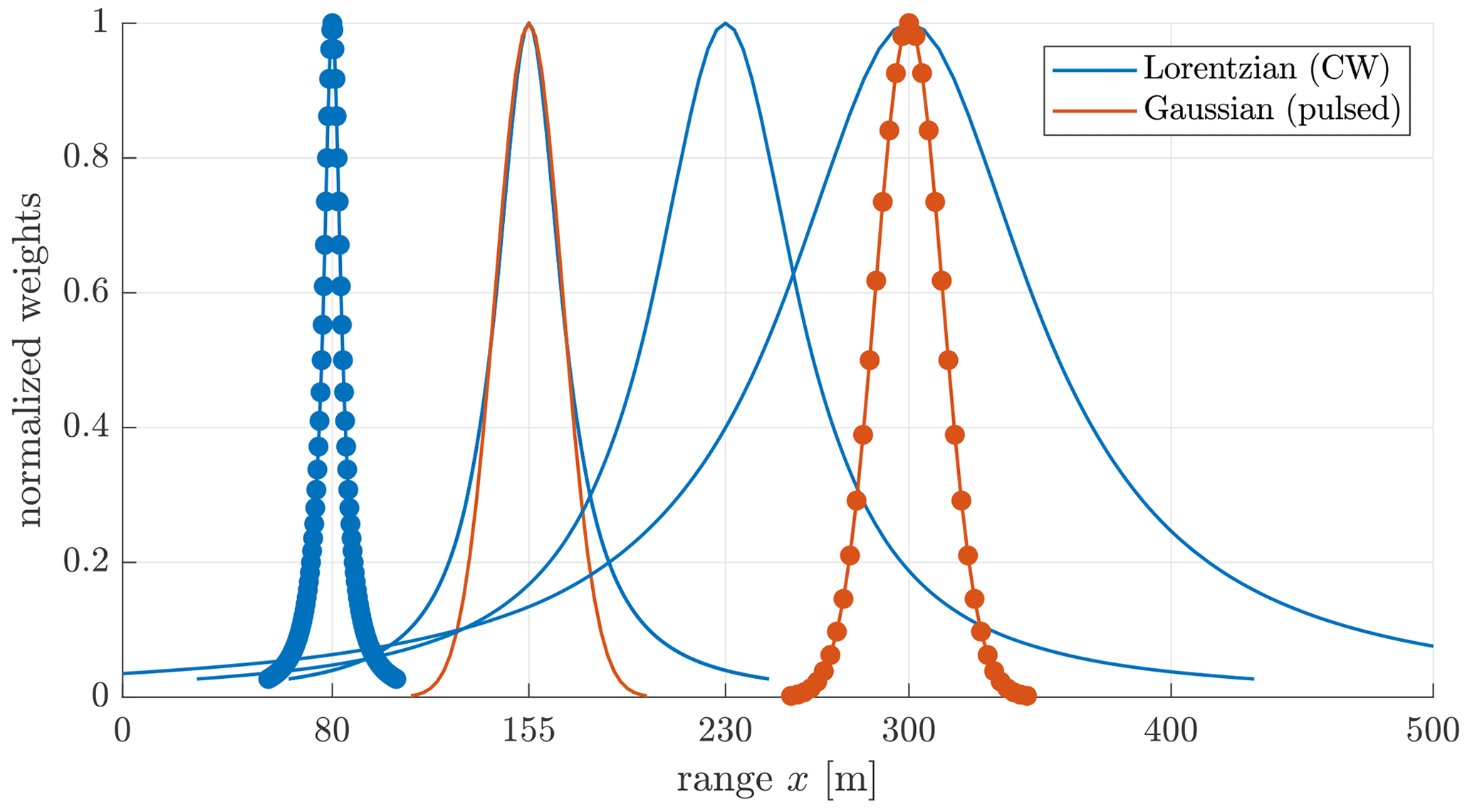
Figure 2Weighting functions of the CW lidar measuring at 80, 155, 230, and 300 m and the one of the pulsed lidar measuring at 155 and 300 m. The weights are normalized by the maximum values for illustration purposes. The blue and red markers indicate the discretization of the functions.
The amount of truncation needs to be balanced between a realistic probe volume and the limited size of the virtual wind fields. The truncation and discretization influence the amount of turbulence attenuation by the probe volume. However, the small turbulent eddies do not greatly impact the coherence of the REWS, since the spatial averaging by the rotor disc has a similar filtering effect on the true REWS.
2.4 Lidar wind preview quality
2.4.1 Rotor-effective wind speed from the wind turbine
If the yaw misalignment is neglected, the true REWS is the spatial average of the longitudinal velocities u across the rotor-swept area defined by the rotor radius R (Schlipf et al., 2015a):
Held and Mann (2019) demonstrated that this REWS can be rewritten as
where , and J1 is the Bessel function of the first kind. Held and Mann (2019) also showed that the auto-spectrum of uRR is
2.4.2 Rotor-effective wind speed estimated by the lidar
Assuming that the turbine yaw misalignment is negligible, the centre line of the lidar scanning trajectory is on the turbine rotation axis, and v and w are considered to be 0, the u component can be estimated directly from the lidar measurements. The lidar-estimated REWS is the mean of the along-wind component retrieved from the radial velocities along the beam:
where Nb is the number of measurements over a full scan, and ni1 is the first element in the unit vector of the ith measurement.
Because the longitudinal wind evolution is the most important factor for control and the considered lidars in this work only measure at a single plane, the wind evolution between each measurement in a full scan is not considered, which should have only a marginal effect on our optimization. The auto-spectrum of the lidar-estimated REWS is (Guo et al., 2022a)
where xi denotes the position vector of the lidar measurement, and nil stands for the lth element in the unit vector n of the ith measurement.
For control purposes, the lidar scanning strategy is considered optimal if it provides REWS estimates that correlate the best with the true REWS sensed by the rotor disc. Considering the turbulence evolution from lidar measurement planes to the rotor plane, the cross-spectrum between uRR and uLL can be expressed as (Guo et al., 2022a)
where Δti denotes the time needed for the turbulence field to travel from a lidar plane to the rotor plane, given a good estimation by their longitudinal separation divided by the mean along-wind speed; i.e. .
2.4.3 Rotor-effective wind speed coherence
The wind preview quality can be evaluated by the magnitude-squared lidar-rotor REWS coherence as follows (Schlipf, 2016; Simley et al., 2018):
which has a value between 0 and 1. The measurement coherence bandwidth (MCB) is defined as the wave number k0.5, where drops below 0.5. The corresponding frequency can be calculated by . The larger the MCB, the better the wind preview quality. Therefore, maximizing the MCB is the goal of lidar trajectory optimization.
To evaluate the lidar wind preview quality, the so-called “smallest detectable eddy size” deddy,min is used by control engineers, which is the size of the eddies that can still be detectable by the lidar with the 50 % coherence assuming turbulence isotropy (Schlipf et al., 2018):
The smallest detectable eddy size is inversely proportional to the MCB. To have a measure that is independent of the rotor size, deddy,min can be normalized by the rotor diameter of the reference wind turbine. A normalized deddy,min close to 1 D indicates a very good lidar configuration for the purpose of fatigue load reduction, while a value between 1.5 and 2 D is satisfying.
The wind preview quality of the considered lidar configurations is directly calculated for the reference wind turbine in the frequency domain using Eqs. (22), (24), and (25) instead of using time-domain simulations, which greatly reduces the computational effort and provides a more accurate MCB value compared to that estimated from simulated spectra of coherence in the time domain. Then, the controller performance using the optimal lidar configurations is evaluated using time-domain aero-elastic simulations with Mann turbulent wind fields.
3.1 Simulation environment
The time-domain aero-elastic simulations are performed for the IEA 15 MW wind turbine using the open-source tool OpenFAST (National Renewable Energy Laboratory, 2022), in which a lidar simulator is embedded. Using the latest version of the OpenFAST lidar simulator (see Guo et al., 2022b, for more details), the probe volume, turbine nacelle motion, and turbulence evolution are included. The weighting function of the probe volume is given in discrete points as explained in Sect. 2.3.
The 4D stochastic turbulence fields are generated by the 4D Mann turbulence generator developed by Guo et al. (2022a). The turbulence fields have model parameters m s−2, L=49 m, and Γ=3.1, which are typical of near-neutral atmospheric conditions and correspond to the IEC class 1B with a turbulence intensity of ≈15 % at a mean wind speed of 18 m s−1. The mean wind field at the turbine hub height and a power-law shear profile with a shear exponent of 0.14, i.e. , are added onto the turbulence boxes, where zHH is the turbine hub height. The turbulence box has dimensions of grid points in the x, y, and z directions, respectively. The grid sizes in the y and z directions are both 4.5 m to cover the whole rotor disc and the tower in the vertical direction, while the resolution in the x direction is Δx=0.5Uref. All simulations are performed for a single wind speed of Uref=18 m s−1. The blade, tower, and generator degree of freedoms (DOFs) are enabled.
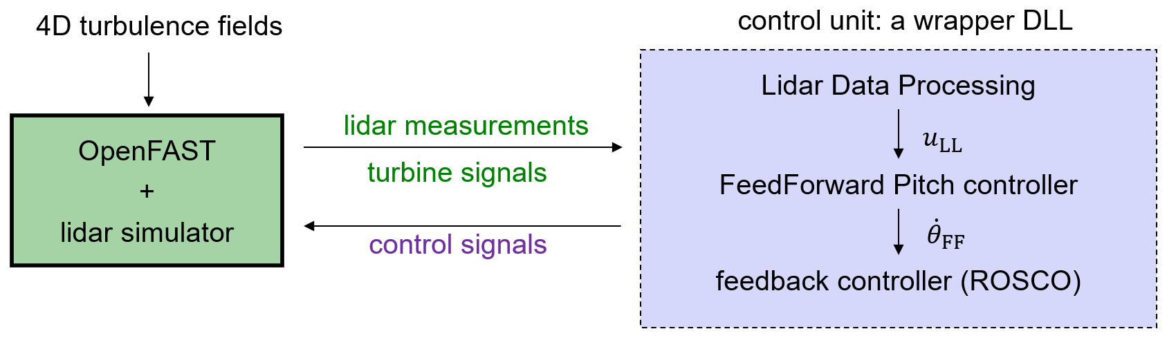
Figure 3Structure of the communication interface between OpenFAST and the controller dynamic-link library chain.
As illustrated in Fig. 3, the turbulent wind disturbs the turbine. The turbine-lidar unit delivers lidar radial velocities and simultaneous turbine signals (generator speed and pitch angle) to the control unit, which then sends control signals (generator torque and demanded pitch angle) back to the turbine to demand control actions. Therefore, without the feedforward controller that relies on the wind preview, the feedback controller calculates control demands based on the past turbine signals and reacts to the disturbance only after the aerodynamic impact on the turbine structure has occurred. The feedforward controller utilizes the lidar-estimated preview information and assists the feedback controller to react in advance. Since OpenFAST can only refer to a single dynamic-link library (DLL) as the control unit, a wrapper DLL is configured to encapsulate and call the lidar data processing, feedforward pitch controller, and feedback controller (ROSCO; Abbas et al., 2022) sequentially in order to exchange signals with OpenFAST (Guo et al., 2023). The three subunits are introduced in the following subsections.
3.2 Lidar data processing
The simulated spinner-based lidar completes a full scan in approximately 8 s with a sampling frequency of 4 Hz. Therefore, the latest 32 measurements are collected to reconstruct the REWS using Eq. (23), and the reconstructed REWS is updated every 0.25 s. In frequency-domain optimization, the beam scanning locations in the circular pattern are assumed to be fixed, while in time-domain simulations, the beam scanning locations depend on the rotor azimuth positions and nacelle motions in real time.
In practice, the REWS estimated from the lidar measurements is not perfectly correlated with the real one sensed by the rotor. Therefore, a filter needs to be applied to the lidar-estimated REWS before using it for the feedforward controller to avoid unnecessary and harmful reactions from the pitch actuator. Here, a first-order Butterworth low-pass filter is applied:
with a cutoff angular frequency , which is calculated from the cutoff wavenumber kcutoff, where the theoretical REWS measurement transfer function drops at −3 dB (Schlipf, 2016; Guo et al., 2023) and s is the complex frequency. The theoretical REWS transfer function is calculated from Eqs. (25) and (24):
The low-pass filtering usually delays a signal due to the frequency-depending phase shift. For the first-order filter, the time delay Tfilter is approximated by
where fdelay is the interested frequency in which the simulated rotor speed spectrum by the feedback-only control has its highest energy. Here, we use fdelay=0.025 Hz for the IEA 15 MW monopile offshore wind turbine as in Schlipf et al. (2023). Therefore, as the cutoff frequency increases, more useful information becomes available in the lidar-estimated REWS signals, reducing the time needed for filtering the signal.
3.3 Feedforward controller
The feedforward controller is designed to stabilize the rotational speed in the changing inflow wind speed by demanding an additional pitch angle θFF before the disturbance hits the rotor. In this way, the rotor speed acceleration caused by the wind speed fluctuations can be compensated for by the additional pitch angle.
The design of the feedforward controller follows the methodology given in Schlipf (2016) and Guo et al. (2023). Considering a reduced-order model of the direct-drive IEA 15 MW wind turbine (National Renewable Energy Laboratory, 2020) with a single rotor rotation DOF,
with
where J is the rotor inertia, θp is the blade pitch angle, cP is the turbine power coefficient, λ is the tip speed ratio, Ma is the aerodynamic torque, and MG is the generator torque. The aerodynamic effect on the rotational speed change can be cancelled out if . Therefore, by changing the pitch angle, the aerodynamic torque is adjusted to be close to the rated value of the generator torque. The feedforward pitch angle θFF should follow the static pitch curve , which can be obtained by steady-state simulations with a feedback controller and the uniform and constant wind of all speeds between cut-in and cutoff, as shown in Fig. 4. At the cut-in wind speed, the blades have an initial pitch angle. The pitch angle first decreases to make the best use of the incoming wind and increases after reaching the rated wind speed of 10.59 m s−1. Here, we only use the static pitch curve above the rated wind. The feedforward pitch angle is obtained by interpolating the static pitch curve in every simulation time step. As described in Schlipf (2016) (see Sect. 6.1.1 for more details), using a feedforward pitch rate instead of the feedforward pitch angle has advantages for the implementation of the feedback–feedforward combined controller. Therefore, we use a simple time derivative of the feedforward pitch angle to obtain the feedforward pitch rate and then add the pitch rate to the integrator input of the feedback controller.
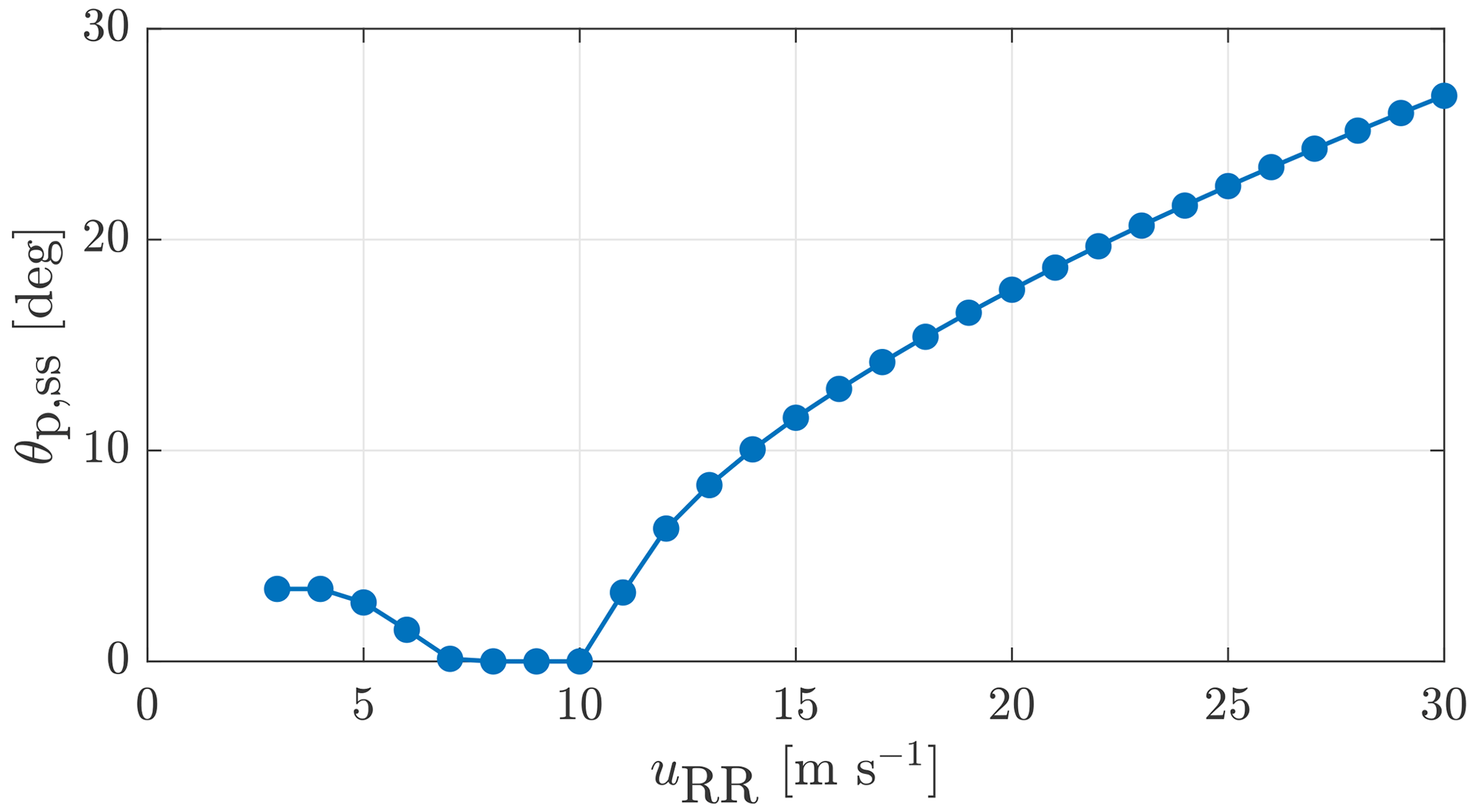
Figure 4Static pitch curve of the bottom-fixed IEA 15 MW wind turbine performed with ROSCO in OpenFAST.
3.4 Feedback controller
The modular Reference Open-Source COntroller (ROSCO) developed by Abbas et al. (2022) for fixed and floating wind turbines is used as the feedback controller in this work. The feedback controller contains two parts: a torque controller, which mainly regulates the generator torque MG to maximize the energy yield in below-rated wind speeds and keeps the power steady in above-rated wind speeds, and a collective blade pitch controller, which maintains the rated generator speed in the fluctuating wind by changing the blade pitch angle.
The baseline collective blade pitch controller is achieved by a proportional–integral (PI) controller described in Jonkman et al. (2009). Therefore, the calculated pitch angle is
where kp is the proportional gain, ki the integral gain, the difference between the contemporary generator speed and its rated value, and s the complex frequency. The default values of the feedback controller gains are used in this study.
The integral block of the feedback controller uses the feedforward pitch rate passed by the feedforward controller. This gives the total demanded pitch angle θc as
Then, the pitch actuator moves the blades according to the demanded pitch angle. The pitch actuator is modelled as a second-order damper system with a cutoff frequency of 1.5708 rad s−1 and a damping ratio of 0.707, which are based on the values of the ROSCO designed for the IEA 15 MW wind turbine (Abbas et al., 2022). Therefore, the pitch actuation takes Tpitch≈0.9 s for frequencies lower than 0.04 Hz for the reference wind turbine.
3.5 Buffer time of REWS signal
To synchronize the pitch actuation with the REWS interacting with the turbine, the preview signal is usually buffered with a suitable time Tbuffer. Tbuffer is calculated from the advection time of the wind field from the lidar measurement plane to the rotor plane , the averaging time of the lidar raw measurement (half of a full scan time Tscan), the time consumed by the low-pass filter Tfilter, and the pitch actuator delay Tpitch (Schlipf, 2016):
To ensure the feedback–feedforward combined controller has enough time to react to the wind disturbance before the wind hits the rotor, Tbuffer has to be larger than or equal to 0. Since Tlead and Tfilter are influenced by the lidar scanning trajectory, Tbuffer≥0 s is a constraint to select the optimal configuration.
We optimize the scanning locations of the spinner-based single-beam lidar to achieve the best wind preview quality. The optimization problem can be formulated as
which uses the measurement range x and the lidar half-cone opening angle ϕ as the optimization variables, MCB as the cost function, and a positive buffer time as the constraint. The optimization problem is solved by brutal-force optimization.
Based on the coherence model given in Sect. 2.4, we calculate the analytical MCB (also written as k0.5) in the frequency domain for different combinations of the lidar measurement range along the x direction and the half-cone opening angle ϕ. The focus distance can be calculated from the measurement range by . For simplicity, only a single measurement range is considered for both CW and pulsed lidars in this work, although measurements from multiple ranges can be obtained simultaneously using pulsed lidars. The lidar configuration is considered to be optimal when the highest MCB is achieved. Meanwhile, the selected lidar configuration needs to give a positive buffer time, as described in Sect. 3.5, so that the controllers have enough time to react to the changing wind.
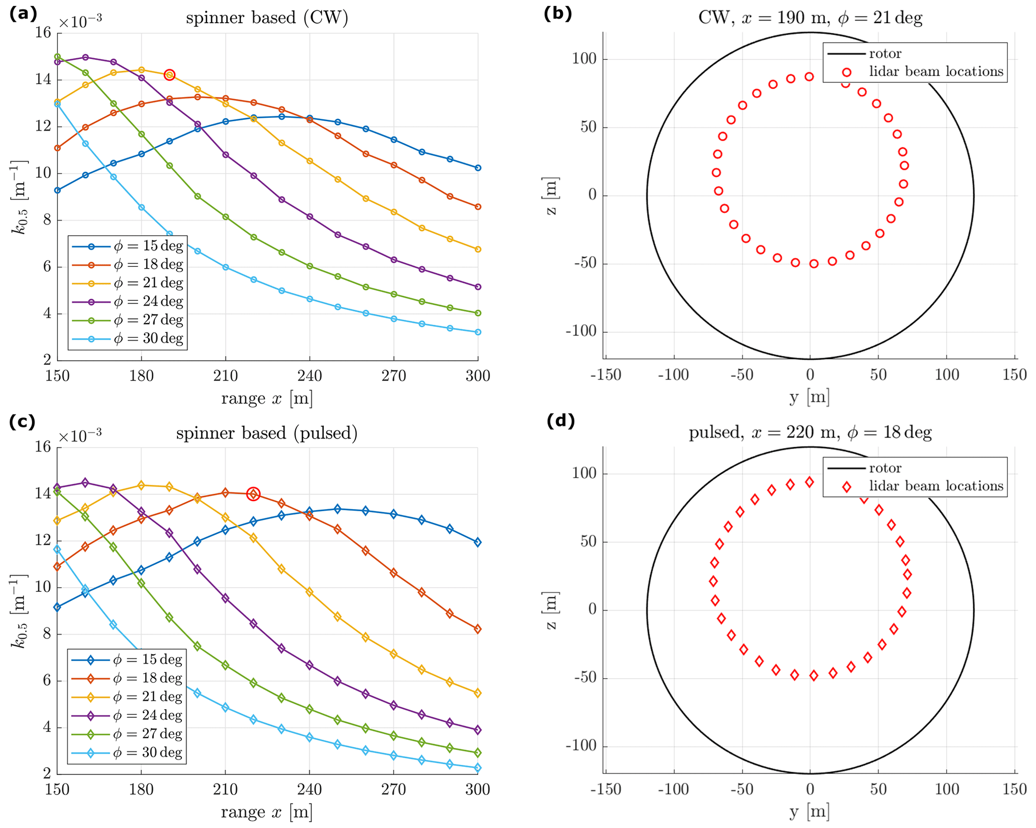
Figure 5(a, c) Optimization of the range x and half-cone opening angle ϕ of the spinner-based lidar based on a coherence model. The mean wind speed is 18 m s−1. The selected optimum configurations are marked in the red circle. (b, d) The scanning pattern of the selected optimum configurations.
The optimization is done assuming a mean wind speed of 18 m s−1. The optimization results are shown in Fig. 5a and c for CW and pulsed spinner-based lidars, respectively. Although measuring at 160 m and ϕ=24∘ with a CW lidar provides the highest MCB in our optimization, it is not usable due to a negative buffer time. Therefore, the optimum scanning configuration of the single-beam lidar in a CW system is selected at x=190 m and ϕ=21∘, and the one for the pulsed system is at x=220 m and ϕ=18∘. We see that the CW lidar gives a better wind preview when it measures closer to the rotor with a wider angle compared to the pulsed lidar. This is expected since the further the CW lidar measures, the larger the lidar probe volume, whereas the probe volume of the pulse lidar does not change with its measurement range. The probe volume filtering effect (along with other effects, such as wind evolution) contributes to the decrease in MCB with increasing measurement distance.
The best range-opening angle combinations of both CW and pulsed lidars result in a scan radius at approximately 72 m (0.6 R) (see Fig. 5b and d). Due to the rotor shaft tilt angle, the lidar scanning area is at the middle–top part of the rotor plane. With the optimum configuration, both types of spinner-mounted single-beam lidars can achieve a maximum k0.5 of more than 0.014 m−1, corresponding to a deddy,min smaller than 1.87 D, while the nacelle-based single-beam lidar achieves only approximately 0.005 m−1 (the single-point measurements provide a k0.5 that is almost constant but reduces slightly with further measurement ranges).
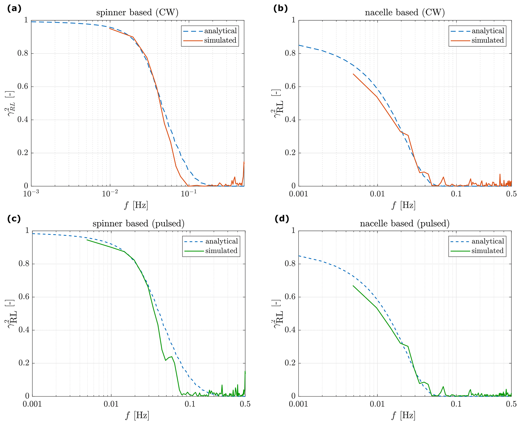
Figure 6Coherence of the REWS using the optimal single-beam lidar (a, c) in the spinner and (b, d) on the nacelle. Upper panel: CW lidars, lower panel: pulsed lidars. The simulation results are averaged from 21 wind field realizations.
With the same turbulence characteristics, the mean wind speed does not have a large impact on the modelling of REWS coherence but is important for the selection of the optimum lidar configurations due to its impact on the buffer time. In our case, the selected configuration of the CW lidar gives a very short buffer time (0.7 s), indicating the measurement distance will be too close for controllers to react if the wind speed is higher than 19 m s−1. Measuring at 220 m and ϕ=18∘ with a pulsed lidar gives a buffer time of 1.62 s, and the controller would have enough time to react for a mean wind speed below 20 m s−1. A larger measurement range should be selected for both types of lidars if the full wind speed range (up to the wind turbine cutoff wind speed of 25 m s−1) is considered. When the measurement range increases from the optimum point, the MCB could decrease. Consequently, the low-pass filter will have a lower cutoff frequency and will need a longer time to process the lidar measurement. Therefore, it is essential to estimate the REWS coherence for the selected scanning pattern and design the control unit accordingly.
Time-domain simulations were executed in OpenFAST with the embedded lidar simulator, the optimal configurations of both lidars given in Fig. 5b and d, the feedback–feedforward controller, and 4D Mann turbulence fields with a mean wind speed of 18 m s−1. To ensure statistical convergence of 10 min simulations, 21 realizations (seeds) of the same turbulence fields are used (Liew and Larsen, 2022). The time series of the filtered REWS uLL is collected from the outputs of the feedforward controller, and the real REWS uRR is calculated from the virtual turbulence fields by averaging the along-wind time series among the rotor-swept area. Simulations with similar set-ups are performed using the nacelle-based lidar. The nacelle-based CW lidar is simulated considering a measurement range of 200 m so that the controller has enough time to react to the turbulent wind with a mean wind speed of 18 m s−1 (it takes longer to filter the REWS signal estimated from the nacelle-based than the spinner-based lidar due to the low MCB). Figure 6 compares the REWS coherence from time-domain simulations and those calculated in the frequency domain using the method presented in Sect. 2.4. Results of the CW and pulsed types of lidar are shown in the upper and lower panels, respectively.
Comparing the left plots (spinner based) with the right plots (nacelle based) in Fig. 6, we see that the coherence in terms of the k0.5 has been improved a lot by using the optimized lidar in the spinner. Overall, the simulated REWS coherence fits with the analytical models, which indicates that the scanning configurations optimized in the frequency domain are also providing the best wind preview in the time domain. Some noise appears at high frequencies due to the spectra estimation process.
The benefits of using the feedforward pitch controller are evaluated in this section. Time-domain simulations are performed using the optimized lidar in the spinner and on the nacelle, first with the feedback controller only and then with the feedback–feedforward combined controller, respectively. Simulations in each scenario are executed using turbulence fields with the same turbulence characteristics for 21 different seeds (Liew and Larsen, 2022). Therefore, for lidar in CW and pulsed systems, simulations are carried out. All DOFs of the 15 MW reference wind turbine are enabled, and no wave impacts are simulated. The simulation time is 640 s in total, in which the first 40 s is the transient and excluded from the analysis. Then, the spectra of the rotor speed, the tower base bending moment, and the blade-root bending moment are calculated from the simulated time series. Here, only results of CW lidars are shown, since similar results are found for pulsed lidars.
The analytical spectrum of the rotor speed using feedforward control is modelled as
where is the closed-loop transfer function from the REWS to the rotor speed, which is obtained from the linearized 1 DOF wind turbine model with the feedback controller (PI), the low-pass filter, and the pitch actuator (Schlipf et al., 2015b).
Results are shown in Fig. 7, in which the left panels are from the spinner-based lidar and the right panels from the nacelle-based lidar. The benefits of using feedback–feedforward control (FBFF) compared to the feedback-only (FB-only) case are clearly visible mainly at low frequencies. This is expected since the low-frequency range is where the lidar wind preview signal correlates well with the real REWS. In Fig. 7a and b, the simulated rotor speed spectra fit well with the analytical spectra for the frequency range below 0.2 Hz (below the 1P of the turbine). Significant reductions in the rotor speed variations are achieved using the spinner-based configuration compared to the nacelle-based one. Furthermore, within the low-frequency range, higher load reductions in the tower-base fore–aft (below 0.07 Hz) and blade-root flapwise directions (below 0.1 Hz) can be seen using the spinner-based lidar.
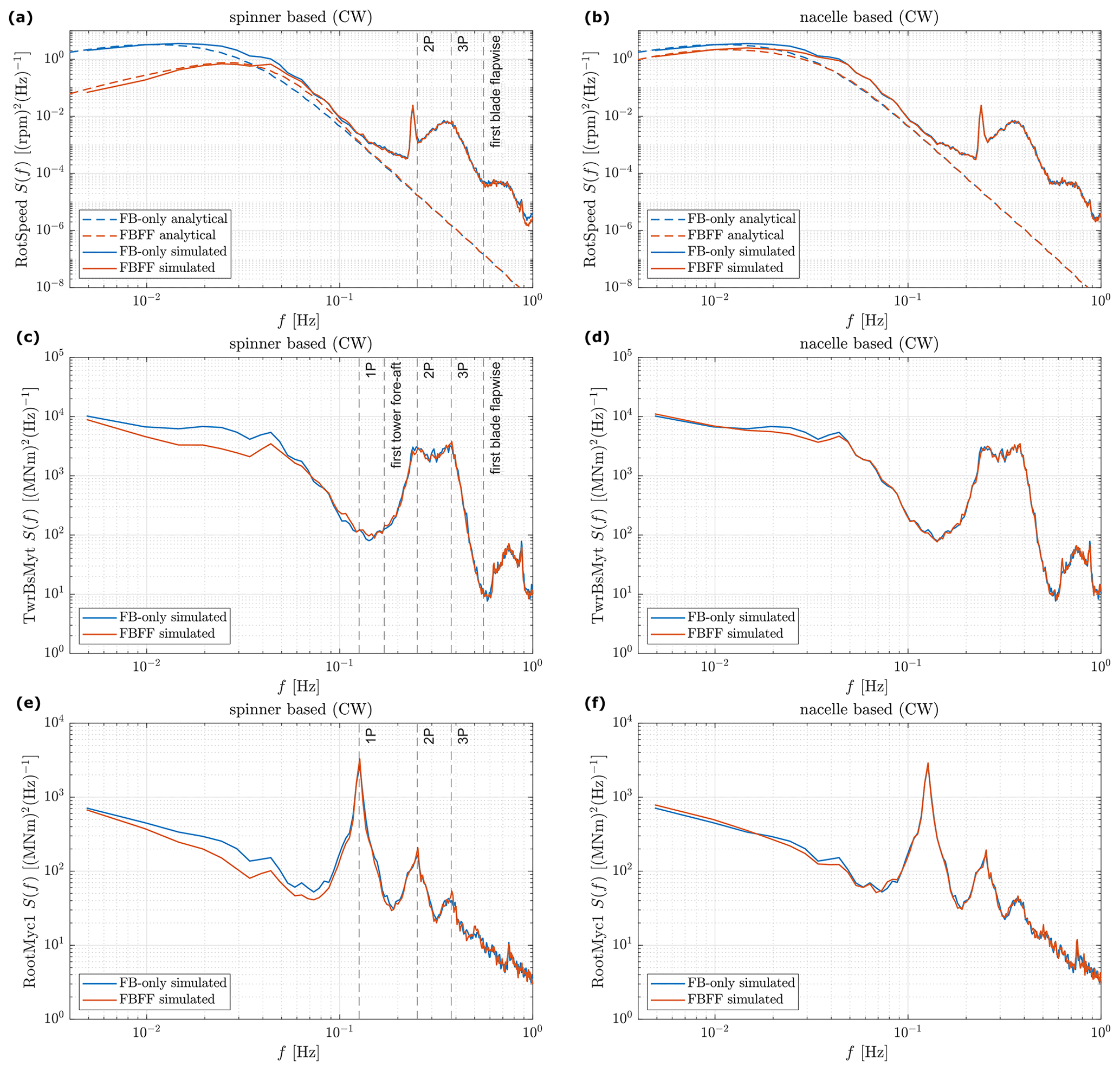
Figure 7Spectra of the rotor speed (RotSpeed), tower-base fore–aft (TwBsMyt), and blade-root flapwise bending moments (RootMyc1) with the feedback-only (FB) and feedback–feedforward combined (FBFF) controller using the optimal single-beam CW lidar (a, c, e) in the spinner and (b, d, f) on the nacelle at a mean wind speed of 18 m s−1. Simulation results are the average using 21 wind field realizations. Some relevant structural frequencies are marked.
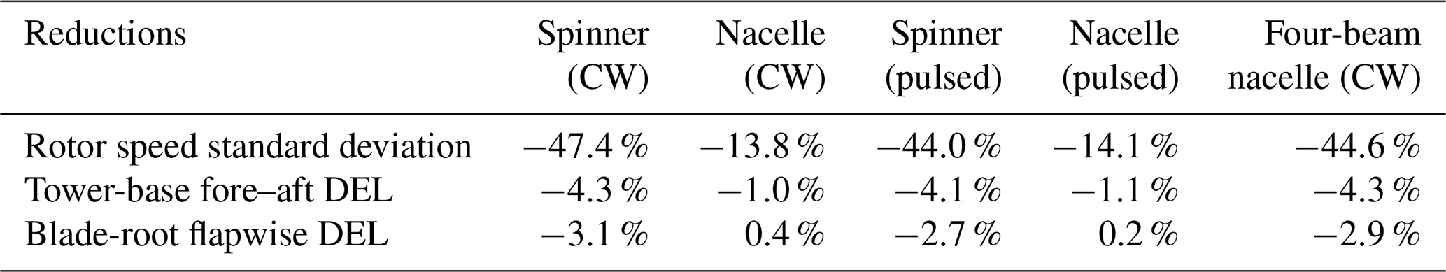
The standard deviation of the rotor speed and the fatigue loads, i.e. damage equivalent loads (DELs), of the tower-base and blade-root bending moments are calculated from the time series. To estimate the DELs, the rainflow-counting method introduced by Matsuichi and Endo (1968) is applied. The DELs are based on a reference number of cycles of 2×10⁶ and a turbine lifetime of 20 years. Wöhler exponents of 4 and 10 are used for the tower-base fore–aft and blade-root flapwise bending moments, respectively, as described in Schlipf (2016). Statistically, by using FBFF with the single-beam CW lidar in the spinner instead of on the nacelle, the reduction in the mean rotor speed standard deviation is improved from 13.8 % to 47.4 %, and the reduction in the tower-base fore–aft bending moment DEL increases from 1.0 % to 4.3 %. The strategy also brings 3.1 % reduction to the blade-root flapwise moment DEL. Since the default feedback controller parameters are adopted, the DEL reductions can be further improved by optimizing the controller gains (Schlipf et al., 2018).
Similar results and trends are seen from the simulations using the pulsed lidar, which are summarized in Table 1. We have also optimized the scanning pattern of a four-beam CW nacelle lidar, which provides an MCB of around 0.011 m−1 measuring at 220 m with ϕ=15∘. The optimized four-beam nacelle lidar is applied and simulated with 21 realizations of the same turbulence fields. The results in Table 1 show that the control benefits gained using the spinner-based single-beam lidar are more than those we can achieve using the same lidar on the nacelle and that the benefits using a spinner-beam single-lidar are on a similar level to those using a four-beam system.
Table 1Control benefits of feedback–feedforward combined controllers relative to using feedback-only controllers for a single-beam lidar in the spinner and on the nacelle, both using a CW and a pulsed system, and a four-beam CW lidar on the nacelle at a mean wind speed of 18 m s−1.
The goal of this study is to demonstrate that a single-beam lidar mounted in the spinner increases the performance of feedforward control compared to the same lidar mounted on the nacelle. The study optimizes the lidar scanning configurations for the best wind preview quality considering the longitudinal wind evolution in the wind field. The optimum configurations for both CW and pulsed lidars are selected for a mean wind speed of 18 m s−1.
The strength of wind evolution is one of the factors that affect the optimal lidar scanning configuration. Other factors include the number and the location of measurements; the turbulence spectra; and the severity of contamination by the transverse velocity components, which is affected by the lidar beam directions (Guo et al., 2022a). The smaller the beam opening angle, the smaller the contribution of the transverse velocity components to the radial velocity. To reveal the impact of turbulence evolution, Fig. 8 shows the optimization results of the CW and pulsed lidars when the evolution is neglected and Taylor's frozen-turbulence hypothesis is applied. Compared to those shown in Fig. 5, the maximum achievable MCBs of both lidars are overestimated for the CW lidar, assuming frozen turbulence does not change the shape of the MCB curve. This is expected because the probe volume of a CW lidar increases quadratically with the focus distance, which plays a more important role in determining the MCBs than the turbulence evolution. As for the pulsed lidar, whose probe volume does not change with the measurement range, the highest MCB is reached at a further measurement distance at x=270 m and a smaller opening angle compared to the optimum in Fig. 5. The resulting lidar scan radius remains at ≈0.6R. Owing to the rotor shaft tilt angle, measuring too far away from the rotor easily causes the lidar scanning area to be out of the rotor-swept area. Therefore, the MCB decreases from the optimum point when the lidar measures at x=270 m with a wider opening angle or with ϕ=15∘ at a further measurement distance. In summary, the neglection of wind evolution can result in an overestimation of MCB; wrong selection of the optimum lidar configuration; and eventually the underperformance of the feedforward control, especially in unstable atmospheric conditions.
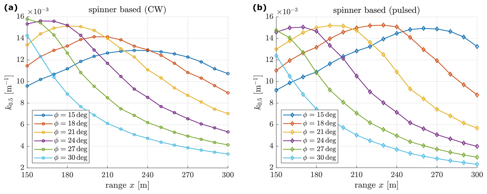
Figure 8Optimization of the range x and half-cone opening angle ϕ of the spinner-based lidar when wind evolution is neglected.
As mentioned in Sect. 4, for higher wind speeds, larger measurement ranges are needed for both CW and pulsed lidars so that the controllers have enough time to react to the wind disturbance. Further work needs to be done with the full wind speed range to decide on the best scanning configuration of the single-beam lidar in the spinner. Also, the controller performances can be influenced by turbulence conditions. Only neutral atmospheric stability is considered in this work. Guo et al. (2023) showed that the control benefit is at its highest in unstable atmospheric conditions, in the middle in neutral atmospheric conditions, and at its lowest in stable atmospheric conditions.
A single-beam Doppler lidar is flexible and low in cost. Using the single-beam lidar in the spinner, the lidar can rotate with the rotor at an almost-steady rotational speed when the turbine operates at above-rated wind speeds and scans a good portion of the inflow to the rotor disc. Also, the spinner-based lidar can have a view of the inflow without periodic blockage by the running blades, which improves the lidar data availability.
Based on a coherence model of the lidar-rotor REWS using the 4D Mann turbulence model, this work optimizes the scanning configurations (i.e. measurement range and the half-cone opening angle) of the spinner-mounted single-beam lidar in a CW and pulsed system, respectively, at a single wind speed of 18 m s−1 for the bottom-fixed IEA 15 MW wind turbine. The optimum configurations of the two types of lidars are different due to the spatial averaging effect of their probe volumes, but they both result in a scan radius of approximately 0.6 of the turbine radius. The optimum configurations of both types of lidars give an MCB of around 0.014 m−1, which corresponds to the smallest detectable eddy size of 1.87 D. Large lidar measurement ranges are needed to ensure the turbine controllers have enough time to react to the wind disturbance over the full wind speed range, which reduces the MCB slightly.
Using time-domain simulations and 4D Mann turbulence wind fields in the neutral condition, the benefits of regulating rotor speed variation and reducing fatigue loads on the tower and blades using the feedforward controller and the spinner-based single-beam lidar are evaluated for the reference turbine at a single wind speed of 18 m s−1. Results are compared against a single-beam and four-beam nacelle-based lidar. The control benefits using the optimized spinner-based configurations of both CW and pulsed lidars are much greater than the single-beam nacelle lidar, and they are on a similar level to the four-beam nacelle lidar.
For future work, full wind speed ranges up to the wind turbine cutoff wind speed should be considered to select the optimum scanning trajectory of the spinner-based single-beam lidar for the IEA 15 MW wind turbine. The pulsed lidar could potentially deliver a better wind preview signal than the one shown in this work when measurements at multiple measurement ranges are combined. In addition, more reductions in fatigue loads could be achieved by optimizing the parameters of the feedback controller. In the future, more than one single-beam lidar can be used in the spinner to add redundancy to the system while having the possibility of achieving a shorter full scan time or multi-plane measurements simultaneously, even with CW lidar systems.
The 4D Mann turbulence generator is accessible via https://doi.org/10.5281/zenodo.7594951 (Guo, 2023a). The source code of the ROSCO controller can be found at https://doi.org/10.5281/zenodo.7594971 (Guo, 2023b), version 2.6.0. The source code and compiled DLLs for the ROSCO feedback controller, the lidar data processing, a collective pitch feedforward controller, and a wrapper DLL are accessible via https://doi.org/10.5281/zenodo.7594961 (Guo, 2023c).
No data sets were used in this article.
All authors participated in the conceptualization and design of the work. FG and WF derived the REWS coherence model. DS and WF designed the lidar-data-processing unit for the spinner-based lidar and did load characterization. WF did lidar optimizations, performed time-domain simulations, and wrote the paper. All authors supported the whole analysis and reviewed and edited the paper.
The contact author has declared that none of the authors has any competing interests.
Publisher's note: Copernicus Publications remains neutral with regard to jurisdictional claims made in the text, published maps, institutional affiliations, or any other geographical representation in this paper. While Copernicus Publications makes every effort to include appropriate place names, the final responsibility lies with the authors.
The authors would like to thank Jakob Mann for the discussion on the modelling of wind evolution and REWS spectra.
This research has been supported by the European Union's Horizon 2020 research and innovation program under the Marie Skłodowska-Curie grant with agreement no. 858358 (LIKE – Lidar Knowledge Europe).
This paper was edited by Jan-Willem van Wingerden and reviewed by Alan Wai Hou Lio and one anonymous referee.
Abbas, N. J., Zalkind, D. S., Pao, L., and Wright, A.: A reference open-source controller for fixed and floating offshore wind turbines, Wind Energ. Sci., 7, 53–73, https://doi.org/10.5194/wes-7-53-2022, 2022. a, b, c, d
Bossanyi, E. A., Kumar, A., and Hugues-Salas, O.: Wind turbine control applications of turbine-mounted LIDAR, J. Phys.: Conf. Ser., 555, 012011, https://doi.org/10.1088/1742-6596/555/1/012011, 2012. a
Canet, H., Loew, S., and Bottasso, C. L.: What are the benefits of lidar-assisted control in the design of a wind turbine?, Wind Energ. Sci., 6, 1325–1340, https://doi.org/10.5194/wes-6-1325-2021, 2021. a
Cariou, J.-P.: Pulsed lidar, in: Remote Sensing for Wind Energy, in: chap. 5, DTU Wind Energy-E-Report-0029(EN), DTU, 104–121, ISBN 978-87-92896-41-4, https://backend.orbit.dtu.dk/ws/portalfiles/portal/55501125/Remote_Sensing_for_Wind_Energy.pdf (last access: 18 December 2023), 2013. a
Fu, W., Peña, A., and Mann, J.: Turbulence statistics from three different nacelle lidars, Wind Energ. Sci., 7, 831–848, https://doi.org/10.5194/wes-7-831-2022, 2022. a
Guo, F.: MSCA-LIKE/4D-Mann-Turbulence-Generator: 4D-Mann-Turbulence-Generator (4D_MannTurbulence_v1), Zenodo [code], https://doi.org/10.5281/zenodo.7594951, 2023a. a
Guo, F.: MSCA-LIKE/OpenFAST3.0_Lidarsim: OpenFAST3.0_Lidarsim (OpenFAST3.0_Lidarsim_v1), Zenodo [code], https://doi.org/10.5281/zenodo.7594971, 2023b. a
Guo, F.: MSCA-LIKE/Baseline-Lidar-assisted-Controller: Baseline-Lidar-assisted-Controller (Baseline-Lidar-assisted-Controllerv_1), Zenodo [code], https://doi.org/10.5281/zenodo.7594961, 2023c. a
Guo, F., Mann, J., Peña, A., Schlipf, D., and Cheng, P. W.: The space-time structure of turbulence for lidar-assisted wind turbine control, Renew. Energy, 195, 293–310, https://doi.org/10.1016/J.RENENE.2022.05.133, 2022a. a, b, c, d, e, f, g, h
Guo, F., Schlipf, D., Zhu, H., Platt, A., Cheng, P. W., and Thomas, F.: Updates on the OpenFAST Lidar Simulator, J. Phys.: Conf. Ser., 2265, 042030, https://doi.org/10.1088/1742-6596/2265/4/042030, 2022b. a, b
Guo, F., Schlipf, D., and Cheng, P. W.: Evaluation of lidar-assisted wind turbine control under various turbulence characteristics, Wind Energ. Sci., 8, 149–171, https://doi.org/10.5194/wes-8-149-2023, 2023. a, b, c, d, e
Harris, M., Hand, M., and Wright, A.: Lidar for Turbine Control: March 1, 2005–November 30, 2005, Tech. rep., OSTI.GOV, https://doi.org/10.2172/881478, 2006a. a
Harris, M., Hand, M., and Wright, A.: Lidar for turbine control, Report No. NREL/TP-500-39154, National Renewable Energy Laboratory, Golden, CO, https://www.nrel.gov/docs/fy06osti/39154.pdf (last access: 18 December 2023), 2006b. a
Held, D. P. and Mann, J.: Comparison of methods to derive radial wind speed from a continuous-wave coherent lidar Doppler spectrum, Atmos. Meas. Tech., 11, 6339–6350, https://doi.org/10.5194/amt-11-6339-2018, 2018. a
Held, D. P. and Mann, J.: Lidar estimation of rotor-effective wind speed – an experimental comparison, Wind Energ. Sci., 4, 421–438, https://doi.org/10.5194/wes-4-421-2019, 2019. a, b
IEC: IEC 61400-1. Wind turbines – Part 1: design guidelines, International standard, International Electrotechnical Commission, Geneva, Switzerland, https://standards.iteh.ai/catalog/standards/sist/3454e370-7ef2-468e-a074-7a5c1c6cb693/iec-61400-1-2019 (last access: 18 December 2023), 2019. a
Jonkman, J., Butterfield, S., Musial, W., and Scott, G.: Definition of a 5-MW Reference Wind Turbine for Offshore System Development, OSTI.GOV, https://doi.org/10.2172/947422, 2009. a
Kumar, A., Bossanyi, E., Scholbrock, A., Fleming, P., Boquet, M., and Krishnamurthy, R.: Field Testing of LIDAR Assisted Feedforward Control Algorithms for Improved Speed Control and Fatigue Load Reduction on a 600 kW Wind Turbine, in: European Wind Energy Association Annual Event, Paris, https://www.researchgate.net/publication/305637934_Field_Testing_of_LIDAR_Assisted_Feedforward_Control_Algorithms_for_Improved_Speed_Control_and_Fatigue_Load_Reduction_on_a_600_kW_Wind_Turbine (last access: 18 December 2023), 2015. a
Liew, J. and Larsen, G. C.: How does the quantity, resolution, and scaling of turbulence boxes affect aeroelastic simulation convergence?, . Phys.: Conf. Ser., 2265, 032049, https://doi.org/10.1088/1742-6596/2265/3/032049, 2022. a, b
Mann, J.: The spatial structure of neutral atmospheric surface-layer turbulence, J. Fluid Mech., 273, 141–168, https://doi.org/10.1017/S0022112094001886, 1994. a
Matsuichi, M. and Endo, T.: Fatigue of metals subjected to varying stress, https://www.semanticscholar.org/paper/Fatigue-of-metals-subjected-to-varying-stress-Matsuichi-Endo/467c88ec1feaa61400ab05fbe8b9f69046e59260 (last access: 18 December 2023), 1968. a
Mikkelsen, T., Angelou, N., Hansen, K., Sjöholm, M., Harris, M., Slinger, C., Hadley, P., Scullion, R., Ellis, G., and Vives, G.: A spinner-integrated wind lidar for enhanced wind turbine control, Wind Energy, 16, 625–643, https://doi.org/10.1002/WE.1564, 2013. a, b
National Renewable Energy Laboratory: Definition of the IEA Wind 15-Megawatt Offshore Reference Wind Turbine, Tech. rep., IEA Wind TCP Task 37, NREL, https://www.nrel.gov/docs/fy20osti/75698.pdf (last access: 18 December 2023), 2020. a, b
National Renewable Energy Laboratory: OpenFAST Documentation, OpenFAST, https://openfast.readthedocs.io/en/main/ (last access: 18 December 2023), 2022. a, b
Peña, A., Floors, R., Sathe, A., Gryning, S. E., Wagner, R., Courtney, M. S., Larsén, X. G., Hahmann, A. N., and Hasager, C. B.: Ten Years of Boundary-Layer and Wind-Power Meteorology at Høvsøre, Denmark, Bound.-Lay. Meteorol., 158, 1–26, https://doi.org/10.1007/s10546-015-0079-8, 2016. a
Schlipf, D.: Lidar-Assisted Control Concepts for Wind Turbines, PhD thesis, Universität Stuttgart, Stuttgart, https://doi.org/10.18419/opus-8796, 2016. a, b, c, d, e, f
Schlipf, D., Fleming, P., Haizmann, F., Scholbrock, A., Hofsäß, M., Wright, A., and Cheng, P. W.: Field testing of feedforward collective pitch control on the CART2 using a nacelle-based lidar scanner, J. Phys.: Conf. Ser., 555, 012090, https://doi.org/10.1088/1742-6596/555/1/012090, 2014. a
Schlipf, D., Haizmann, F., Cosack, N., Siebers, T., and Cheng, P. W.: Detection of wind evolution and lidar trajectory optimization for lidar-assisted wind turbine control, Meteorol. Z., 24, 565–579, 2015a. a, b
Schlipf, D., Simley, E., Lemmer, F., Pao, L., and Cheng, P. W.: Collective Pitch Feedforward Control of Floating Wind Turbines Using Lidar, J. Ocean Wind Energ., 2, 223–230, https://doi.org/10.17736/jowe.2015.arr04, 2015b. a
Schlipf, D., Fürst, H., Raach, S., and Haizmann, F.: Systems Engineering for Lidar-Assisted Control: A Sequential Approach, J. Phys.: Conf. Ser., 1102, 012014, https://doi.org/10.1088/1742-6596/1102/1/012014, 2018. a, b
Schlipf, D., Guo, F., Raach, S., and Lemmer, F.: A Tutorial on Lidar-Assisted Control for Floating Offshore Wind Turbines, in: 2023 American Control Conference (ACC), 31 May–2 June 2023, San Diego, CA, USA, 2536–2541, https://doi.org/10.23919/ACC55779.2023.10156419, 2023. a
Scholbrock, A., Fleming, P., Fingersh, L., Wright, A., Schlipf, D., Haizmann, F., and Belen, F.: Field testing LIDAR-based feed-forward controls on the NREL controls advanced research turbine, 51st AIAA Aerospace Sciences Meeting including the New Horizons Forum and Aerospace Exposition 2013, 7–10 January 2013. Grapevine (Dallas/Ft. Worth Region), Texas, https://doi.org/10.2514/6.2013-818, 2013. a
Scholbrock, A., Fleming, P., Wright, A., Slinger, C., Medley, J., and Harris, M.: Field test results from lidar measured yaw control for improved yaw alignment with the NREL controls advanced research turbine, Tech. rep., NREL, https://www.nrel.gov/docs/fy15osti/63202.pdf (last access: 18 December 2023), 2015. a
Simley, E., Pao, L. Y., Frehlich, R., Jonkman, B., and Kelley, N.: Analysis of light detection and ranging wind speed measurements for wind turbine control, Wind Energy, 17, 413–433, https://doi.org/10.1002/WE.1584, 2014. a, b
Simley, E., Fürst, H., Haizmann, F., and Schlipf, D.: Optimizing lidars for wind turbine control applications-Results from the IEA Wind Task 32 workshop, Remote Sens., 10, 863, https://doi.org/10.3390/rs10060863, 2018. a, b
Sonnenschein, C. M. and Horrigan, F. A.: Signal-to-noise relationships for coaxial systems that heterodyne backscatter from the atmosphere, Appl. Optics, 10, 1600–1604, https://doi.org/10.1364/AO.10.001600, 1971. a
Taylor, G. I.: The spectrum of turbulence, P. Roy. Soc. Lond. A, 164, 476–490, https://doi.org/10.1098/rspa.1938.0032, 1938. a
Venditti, B.: Animation: The World's Biggest Wind Turbines, https://www.visualcapitalist.com/visualizing-the-worlds-biggest-wind-turbines/ (last access: 18 December 2023), 2022. a
- Abstract
- Introduction
- Background
- Time-domain simulation set-up
- Optimization of lidar configuration for wind preview quality
- Feedforward control benefits
- Discussion
- Conclusion and outlook
- Code availability
- Data availability
- Author contributions
- Competing interests
- Disclaimer
- Acknowledgements
- Financial support
- Review statement
- References