Extreme coherent gusts with direction change – probabilistic model, yaw control, and wind turbine loads

Observations of large coherent fluctuations are used to define a probabilistic model of coherent gusts with direction change. The gust model provides the joint description of the gust rise time, amplitude, and directional changes with a 50-year return period. The observed events are from a decade of measurements from a coastal site in western Denmark, making the derived gust model site specific. In conjunction with the gust model, a yaw controller is presented in this study to investigate the load implications of the joint gust variables. These loads are compared with the design load case of the extreme coherent gust with direction change (ECD) from the IEC 61400-1 Ed.4 wind turbine safety standard. Within the framework of our site-specific gust model we find the return period of the ECD to be approximately 460 years. From the simulations we find that for gusts with a relatively long rise time the blade root flapwise bending moment, for example, can be reduced by including the considered yaw controller. From the extreme load comparison of the ECD and the modeled gusts we see that by including the variability in the gust parameters the load values from the modeled gusts are between 20 % and 74 % higher than the IEC gusts.

1 Introduction

In the process of designing a wind turbine, designers have to consider a balance between cost and structural safety. Wind turbine safety standards like the IEC 61400-1 Ed.4 (IEC, 2019) exist to aid designers in ensuring the quality, reliability, and safety of the wind turbine. The IEC standard prescribes extreme external wind conditions which the wind turbine must be able to withstand during the design lifetime, which is at minimum 20 years. The extreme wind conditions are prescribed in a set of models used for specific design load cases (DLCs). The DLCs are used to estimate the structural response to events with a recurrence period of 50 years, which is the intended recurrence period of the environmental conditions prescribed by the IEC standard.

The present study addresses the extreme coherent gust with direction change (ECD) which is used for DLC 1.4 for ultimate load analysis. For certain turbines this load case can drive the ultimate loading of, for example, the blade root flapwise bending moment (Beardsell et al., 2016). The ECD model was originally presented in Stork et al. (1998) and was later validated against measurements and found to give reasonable results in Hansen and Larsen (2007). As pointed out by the authors of Hansen and Larsen (2007), these experiments are based on turbulent fluctuations, where the peak values in the measurements are due to gusts with a limited spatial extent (Larsen et al., 2003). Such gusts are not coherent across the rotor diameter of multi-megawatt wind turbines, like, for example, the DTU 10 MW wind turbine (Bak et al., 2013) that we consider in this study.

In a previous study (Hannesdóttir and Kelly, 2019), observations of coherent ramp-like wind speed fluctuations are detected and characterized. The coherent fluctuations are characterized with rise time, amplitude, and direction change. The observed coherent gusts are further compared with the ECD due to similarities but show a considerable variability in the characterized variables. Generally, the rise time of the observed coherent gusts is much higher than that of the ECD, on average around 200 s. However, the rise-time distribution has a large range. The observed direction change may exceed the one of the ECD, but then the corresponding rise time is considerably longer. In order to simulate a realistic wind turbine response to these observed gusts with long rise times and large direction change, yawing of the wind turbine needs to be included in the simulations.

A yaw controller ensures that the wind turbine is aligned with the mean wind speed direction. Yaw control is important for increasing the power production (Kragh and Hansen, 2015) and for reducing the extreme loading of a turbine operating in yaw misalignment. The yaw controller primarily uses the wind direction as input to determine if the turbine is operating in yaw misalignment. Conventional wind turbines have a wind vane mounted on the nacelle to calculate the yaw error. The positioning of the vane presents uncertainty in the wind direction estimate, since the equipment is installed behind the rotor where the flow is disturbed. Different sensors have been investigated for improved wind direction estimation, e.g., a spinner-mounted, continuous-wave lidar in Kragh et al. (2010). Yaw controllers have been investigated before in connection with energy capture optimization (Bossanyi et al., 2013) but to the authors' knowledge not for investigating extreme loads in conjunction with an aeroelastic code.

The aim of this paper is to investigate how 50-year coherent gusts (based on observations) impact wind turbine loads and how they compare to the DLC 1.4 of the IEC standard. This will be achieved through three steps.

1. Derive a probabilistic gust model by extrapolating the observed gust variables to a 50-year return period. As the gust variables form a 3D space, the extrapolation is done with the Nataf distribution model (Nataf, 1962).

2. Develop a yaw controller to be incorporated in the load simulations, as the observed gusts may have a relatively long rise time, and a real wind turbine could start to yaw under such wind conditions.

3. We simulate thousands of points on the 3D gust variable surface to identify critical load regions. The load simulations are performed using the aeroelastic software HAWC2 (Larsen and Hansen, 2015).

2 The IEC extreme coherent gust with direction change

The amplitude of the extreme coherent gust with direction change (ECD) is V_cg=15 m s⁻¹ and is independent of the 10 min mean hub-height wind speed V_hub. The direction change in the ECD is however a function of V_hub and given by

$$\begin{array}{}\text{(1)}& {\mathit{\theta }}_{\mathrm{cg}}=\left\{\begin{array}{ll}\mathrm{180}{}^{\circ },& \mathrm{if}{V}_{\mathrm{hub}}\le \mathrm{4}\mathrm{m}{\mathrm{s}}^{-\mathrm{1}},\\ \mathrm{720}{}^{\circ }\left(\mathrm{m}{\mathrm{s}}^{-\mathrm{1}}\right)/V_{\mathrm{hub}},& \mathrm{if}\mathrm{4}\mathrm{m}{\mathrm{s}}^{-\mathrm{1}}<V_{\mathrm{hub}}<V_{\mathrm{ref}},\end{array}\right.\end{array}$$

where V_ref is the 10 min mean reference wind speed. The wind speed increase and direction change are assumed to occur simultaneously and are modeled as functions of time,

$$\begin{array}{}\text{(2)}& {\displaystyle }& {\displaystyle }V(z,t)=\left\{\begin{array}{ll}V\left(z\right),& \mathrm{if}t<\mathrm{0}\\ V\left(z\right)+\mathrm{0.5}{V}_{\mathrm{cg}}(\mathrm{1}-\cos (\mathit{\pi }t/T\left)\right),& \mathrm{if}\mathrm{0}\le t\le T\\ V\left(z\right)+V_{\mathrm{cg}},& \mathrm{if}t>T\end{array}\right.,\text{(3)}& {\displaystyle }& {\displaystyle }{\mathit{\theta }}_{\mathrm{cg}}\left(t\right)=\left\{\begin{array}{ll}\mathrm{0}{}^{\circ },& \mathrm{if}t<\mathrm{0}\\ \pm \mathrm{0.5}{\mathit{\theta }}_{\mathrm{cg}}(\mathrm{1}-\cos (\mathit{\pi }t/T\left)\right),& \mathrm{if}\mathrm{0}\le t\le T\\ \pm {\mathit{\theta }}_{\mathrm{cg}},& \mathrm{if}t>T\end{array}\right.,\end{array}$$

where T=10 s is the rise time. The ECD design load case is simulated at three different wind speeds, V_rated (the rated wind speed) and V_rated±2 m s⁻¹ according to the IEC standard. In this study we only simulate the ECD with a starting wind speed of 10 m s⁻¹.

3 Probabilistic model of coherent gusts

In the present study we consider wind speed fluctuations that may be assumed to be coherent across the rotor of any multi-megawatt wind turbine. Such large coherent fluctuations have been detected and characterized in a previous study (Hannesdóttir and Kelly, 2019), where a detailed description of the detection and characterization method may be found. The coherent gusts are detected from a 10.25-year measurement period in Høvsøre, located in western Jutland, Denmark. It is argued that these gusts may originate from a broad variety of phenomena (e.g., convective cells and rolls, shear-driven streaks, gravity waves, pressure disturbances, surface buoyancy fluxes, latent heat release) but share the trait of a ramp-like increase in wind speed that gives rise to extreme 10 min variance. These 10 min extreme wind speed variance events are observed simultaneously (within the same 10 min window) at two meteorological masts that are separated by approximately 400 m, indicating large coherent structures. In brief, the characterization method works in three steps.

• A wavelet transform is made to identify both the exact timing of the wind speed increase and the total length of the time window defined from the wavelet scale.

• An idealized ramp function (a modified error function) is fitted to the measurements within a window defined from the wavelet scale. The parameters from the fit of the ramp function define the rise time (Δt) and amplitude ($\mathrm{\Delta }u=u_{\mathrm{a}}-u_{\mathrm{b}}$), where u_b is the wind speed before the rise and u_a is the wind speed after the rise. The combined duration of u_a, u_b, and Δt is equal to the time window, but their exact individual duration is defined by the ramp function fit.

• The direction change is characterized as the maximum difference in the 30 s moving average directional data during the window defined in the wavelet analysis.

The amplitudes and rise times are estimated from 10 Hz data, measured at three heights: 60, 100, and 160 m. The estimated values are then averaged over the three heights to provide a characteristic amplitude and rise time for each event. The events are observed at wind speeds ranging from u_b=1.4 to u_b=26.4 m s⁻¹. In order to model the gusts, we choose a subset of events with the following selection criteria: u_b<V_rated and u_a>V_rated. In other words, the wind speed is below the rated wind speed before the gust and reaches above the rated wind speed after the gust. This choice of subset is made as high loads are expected to be observed around rated wind speed (Hannesdóttir et al., 2019). A total of 92 events fulfill the selection criteria and are used in the present study.

Figure 1 shows the cumulative distribution function (CDF) of each coherent gust variable Δu, Δθ, and Δt with fitted distributions. The distribution parameters are all found with a maximum likelihood estimation. The gust amplitude Δu is assumed to follow a Gumbel distribution, in which the estimated location and scale parameters are α=6.42 and β=1.77 m s⁻¹. The direction change Δθ is assumed to follow a three-parameter Weibull distribution with the following estimated parameters: k=1.34 (shape parameter), γ=6.37^∘ (location parameter), and A=25.30^∘ (scale parameter). The rise time is assumed to follow the reversed two-parameter Weibull distribution, in which the estimated parameters are k=1.47 and A=279.37 s. Note that we change the sign of the rise time when fitting the reversed Weibull distribution. This is done to ensure that the short rise times are defined as extreme values.

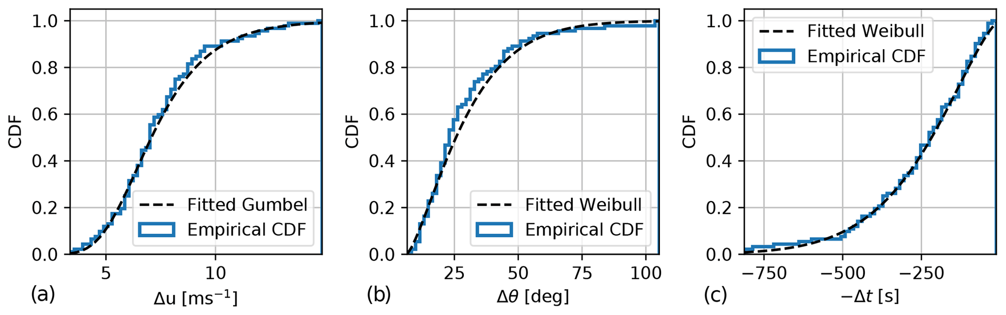
Figure 1 The marginal fitted and empirical cumulative distributions of gust amplitude (a), gust direction change (b), and negative gust rise time (c).

3.1 Inverse second-order reliability method with the Nataf distribution model

In this section we derive an environmental surface that provides the 50-year return period of the joint coherent gust variables, Δu, Δθ, and Δt. Traditionally, the inverse first-order reliability method (IFORM) (Winterstein et al., 1993) is used within wind energy to predict such extreme environmental conditions, e.g., for the 50-year return period of the joint description of wind speed and turbulence levels (Fitzwater et al., 2003; Sang Moon et al., 2014; Dimitrov et al., 2017). It has however recently been shown that the IFORM does not account for the whole probability space outside the surface when defining the exceedance probability (Chai and Leira, 2018; Dimitrov, 2020). In fact, the notion of exceedance probability with the IFORM corresponds to a marginal exceedance probability (Mackay and Haselsteiner, 2021). But in our study, we wish to define the exceedance probability in terms of the whole probability space outside the environmental surface; i.e., a gust with environmental variables beyond the 50-year return period surface should statistically represent a 50-year event. Using the IFORM is therefore not suited for our desired definition of a 50-year event and would lead to a non-conservative return period prediction. Instead we choose to use the inverse second-order reliability method (ISORM) (Chai and Leira, 2018), in which exceedance probability is defined to be anywhere beyond the return period surface. The method follows the same general procedure and steps of the IFORM except for when the so-called “reliability index” is calculated (see Eq. 6 below).

Here the joint probability distribution of the variables is given by the Nataf distribution model, which is defined by Liu and Der Kiureghian (1986). Under Nataf transformation (Nataf, 1962), the considered variables are mapped from original space into correlated standard normal space, in which the joint description of the variables is defined by a Gaussian copula. Unlike the Rosenblatt transformation (Rosenblatt, 1952), which is exact, the Nataf transformation is an approximation. In order to perform the Rosenblatt transformation, the complete joint cumulative distribution of the variables is needed, which is not available for the current analysis. However, to perform the Nataf transformation it is enough to know the marginal distributions and the correlation matrix of the variables.

The Nataf transformation of a random vector X=X₁, …, X_n to standard normal space is performed by

$$\begin{array}{}\text{(4)}& Z_i={\mathrm{\Phi }}^{-\mathrm{1}}\left(F_{x_i}\left(X_i\right)\right),i=\mathrm{1},\mathrm{\dots },n,\end{array}$$

where Φ⁻¹ is the inverse standard normal CDF and $F_{x_i}\left(X_i\right)$ is the marginal CDF of X_i. The standard normal vector Z=Z₁, …, Z_n has a correlation matrix ρ₀.

3.1.1 Constructing the environmental surface

The first step in constructing the environmental surface of coherent gust variables is to calculate the exceedance probability (P_e) associated with the 50-year return period of an observed coherent gust. When the data have a regular time step, the probability of a single 10 min measurement to exceed the 50-year value is $P_{\mathrm{50}}=T_{\mathrm{0}}/T_{\mathrm{50}}$, where T₀ is a 10 min reference period and T₅₀ is the 50-year return period with the same unit as the reference period. However, as the coherent gusts do not occur with a regular time step, the exceedance probability has to be adjusted with the annual exceedance frequency of the detected coherent gusts $f_{\mathrm{a}}=n_{\mathrm{cg}}\cdot T_{\mathrm{0}}/T_{\mathrm{m}}$, where n_cg is the total number of observed coherent gusts and T_m is the measurement period converted to the same unit as the reference period. There are 92 selected coherent gusts found from 10 min samples spanning a 10.25-year period, giving the following exceedance probability:

$$\begin{array}{}\text{(5)}& P_{\mathrm{e}}={\displaystyle \frac{P_{\mathrm{50}}}{f_{\mathrm{a}}}}={\displaystyle \frac{\mathrm{1}}{\mathrm{50}\cdot (\mathrm{92}/\mathrm{10.25})}}=\mathrm{0.0022}.\end{array}$$

The next step is to find the associated reliability index, which has its name from the traditional first-order reliability method (Ditlevsen and Madsen, 1996) and defines the distance from the origin (in standard normal space) to the “limit state surface”. Following the ISORM methodology, the reliability index is defined by

$$\begin{array}{}\text{(6)}& \mathit{\beta }=\sqrt{{\left[{\mathit{\chi }}_k^{\mathrm{2}}\right]}^{-\mathrm{1}}\left(\mathrm{1}-P_{\mathrm{e}}\right)}=\mathrm{3.82},\end{array}$$

where $[{\mathit{\chi }}_k^{\mathrm{2}}{]}^{-\mathrm{1}}$ is the inverse CDF of the χ² distribution with k degrees of freedom. Here we use k=3 because we have a 3D gust variable space. Note that with the IFORM, the reliability index is defined as $\mathit{\beta }={\mathrm{\Phi }}^{-\mathrm{1}}(\mathrm{1}-P_{\mathrm{e}})$. In standard normal space β defines the radius of a sphere,

$$\begin{array}{}\text{(7)}& \mathit{\beta }=\sqrt{u_{\mathrm{1}}^{\mathrm{2}}+u_{\mathrm{2}}^{\mathrm{2}}+u_{\mathrm{3}}^{\mathrm{2}}},\end{array}$$

where u₁, u₂, and u₃ are spherical coordinates of the vector $\left|\mathit{U}\right|=\mathit{\beta }$. The spherical coordinates may be generated by

$$\begin{array}{}\text{(8)}& {\displaystyle }& {\displaystyle }{u}_{\mathrm{1}}=\mathit{\beta }\cos \left(\mathit{\theta }\right)\sin \left(\mathit{\varphi }\right),\text{(9)}& {\displaystyle }& {\displaystyle }{u}_{\mathrm{2}}=\mathit{\beta }\sin \left(\mathit{\theta }\right)\sin \left(\mathit{\varphi }\right),\text{(10)}& {\displaystyle }& {\displaystyle }{u}_{\mathrm{3}}=\mathit{\beta }\cos \left(\mathit{\varphi }\right),\end{array}$$

where $\mathit{\theta }=[\mathrm{0},\mathrm{2}\mathit{\pi }]$ and $\mathit{\varphi }=[\mathrm{0},\mathit{\pi }]$.

Before performing the Nataf transformation, the correlation coefficients of ρ₀ have to be determined. As shown in Liu and Der Kiureghian (1986), the correlation coefficients in standard normal space can be estimated from the correlation coefficients ρ_ij in real space (Δu, Δθ, and Δt) through the following expression:

$$\begin{array}{}\text{(11)}& {\mathit{\rho }}_{\mathrm{0}ij}=E{\mathit{\rho }}_{ij},\end{array}$$

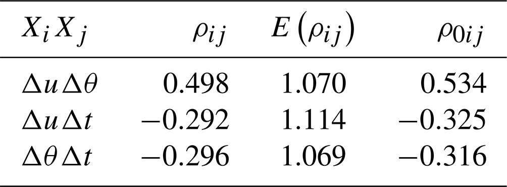
where E≥1 is a function of the correlation coefficient ρ_ij and the corresponding marginal distributions. Empirical expressions for E are provided in Liu and Der Kiureghian (1986) for 10 different distribution functions, in which the Weibull distribution and the Gumbel distribution are both among them. We can therefore use these empirical expressions to estimate E (see Table 1). The correlation coefficients ρ_ij in matrix ρ are calculated in terms of correlation coefficients between X_i and X_j, where X_i is one of the environmental variables: Δu, Δθ, or Δt. The correlation coefficients of matrix ρ₀ are estimated with Eq. (11) (see Table 1).

Table 1 The estimated correlation coefficients and the evaluated empirical expressions for E.

We can now determine ρ₀ as a lower-triangular matrix L₀ by applying Cholesky decomposition. The last step in constructing the environmental surface of coherent gust variables is to apply the inverse Nataf transformation. This is done in two steps: first to transform $\mathit{U}=(u_{\mathrm{1}},u_{\mathrm{2}},u_{\mathrm{3}})$ to the correlated standard normal space,

$$\begin{array}{}\text{(12)}& \mathit{Z}={\mathbf{L}}_{\mathrm{0}}\mathit{U},\end{array}$$

and finally the variables of the surface are found by

$$\begin{array}{}\text{(13)}& {\displaystyle }& {\displaystyle }\mathrm{\Delta }u=F_{\mathrm{\Delta }u}^{-\mathrm{1}}\left(\mathrm{\Phi }\left(Z_{\mathrm{1}}\right)\right),\text{(14)}& {\displaystyle }& {\displaystyle }\mathrm{\Delta }\mathit{\theta }=F_{\mathrm{\Delta }\mathit{\theta }}^{-\mathrm{1}}\left(\mathrm{\Phi }\left(Z_{\mathrm{2}}\right)\right),\text{(15)}& {\displaystyle }& {\displaystyle }\mathrm{\Delta }t=F_{\mathrm{\Delta }t}^{-\mathrm{1}}\left(\mathrm{\Phi }\left(Z_{\mathrm{3}}\right)\right).\end{array}$$

Figure 2 shows the surface of coherent gust variables with a 50-year return period and the 92 coherent gust events used in this analysis. The maximum direction change (Δθ=143.0^∘) and maximum amplitude (Δu=23.5 m s⁻¹) are found on the surface at rise times of 479.4 and 471.0 s respectively. The surface is shown as Δu–Δθ contours for specific rise times in Fig. 3. It can be seen that extreme direction change and amplitude decrease with decreasing rise time. The gray curve shows the Δu−Δθ contour where the rise time matches the rise time of the ECD, Δt=10 s. On that curve we find the maximum Δu=13.1 m s⁻¹ and the maximum Δθ=75.4^∘.

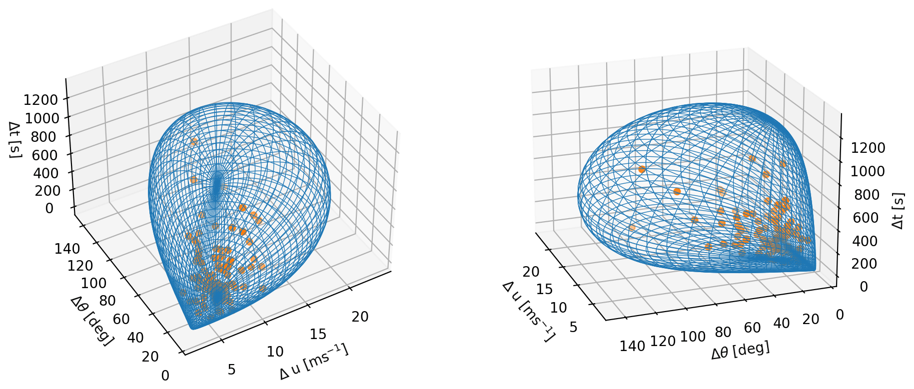
Figure 2 The 50-year return period surface of Δu, Δθ, and Δt, seen from two different angles and the 92 coherent gust events.

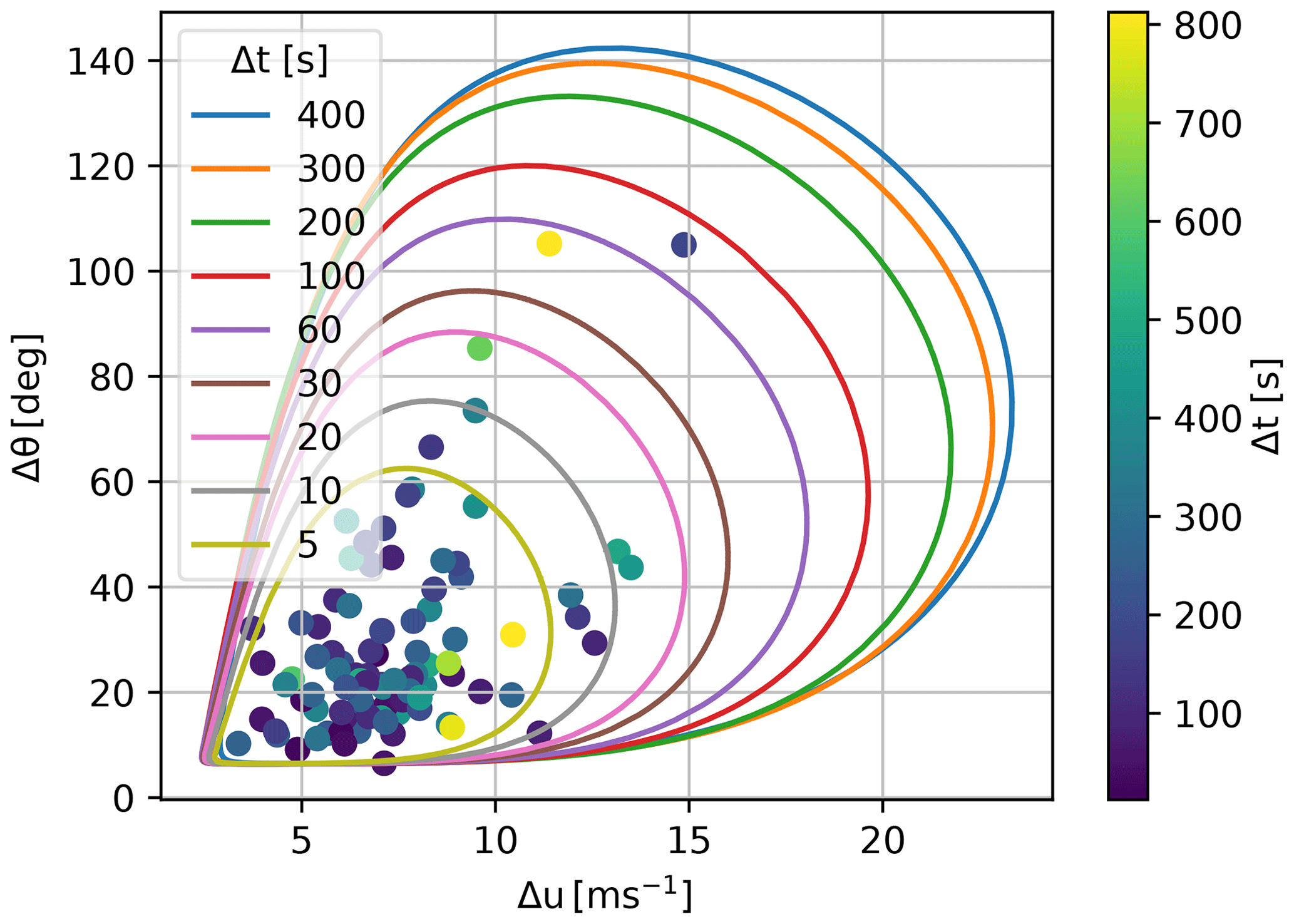
Figure 3 The 50-year return period surface, sliced at different rise times. The color scale shows the rise time for the 92 coherent gust events.

3.1.2 The return period of the IEC ECD

We see from the gust variables on the 10 s rise-time contour in Fig. 3 that if we match the direction change in the ECD (Δθ=72^∘), the amplitude is significantly lower, Δu=10.0 m s⁻¹. One could then ask the following: what is the required return period of the ECD gust parameters when considered within this framework? In other words, what return period do we have to use in order to make a point on the surface match all three ECD variable values? The answer to that question may be found by doing the reversed operation of constructing the environmental surface:

$$\begin{array}{}\text{(16)}& {\mathit{Z}}_{\mathrm{ECD}}=\left\{\begin{array}{l}{\mathrm{\Phi }}^{-\mathrm{1}}\left(F_{\mathrm{\Delta }u}\left(\mathrm{15}\right)\right)\\ {\mathrm{\Phi }}^{-\mathrm{1}}\left(F_{\mathrm{\Delta }\mathit{\theta }}\left(\mathrm{72}\right)\right)\\ {\mathrm{\Phi }}^{-\mathrm{1}}\left(F_{\mathrm{\Delta }t}\left(\mathrm{10}\right)\right)\end{array}\right.,\end{array}$$

followed by the step

$$\begin{array}{}\text{(17)}& {\mathit{U}}_{\mathrm{ECD}}={\mathbf{L}}_{\mathrm{0}}^{-\mathrm{1}}{\mathit{Z}}_{\mathrm{ECD}}.\end{array}$$

The reliability index may be found by ${\mathit{\beta }}_{\mathrm{ECD}}=\left|{\mathit{U}}_{\mathrm{ECD}}\right|$ and the associated probability by $P_{\mathrm{ECD}}=\mathrm{1}-D_k\left({\mathit{\beta }}_{\mathrm{ECD}}^{\mathrm{2}}\right)$. Finally the return period is found:

$$\begin{array}{}\text{(18)}& T_{\mathrm{ECD}}={\displaystyle \frac{\mathrm{1}}{P_{\mathrm{ECD}}\cdot \mathrm{92}/\mathrm{10.25}\mathrm{years}}}=\mathrm{460.4}\mathrm{years}.\end{array}$$

A return period of 460 years is an order of magnitude larger than the usual 50-year return period used in wind turbine design. The reason for this large return period is that, according to our distributions and correlations between the coherent gust variables, there is a low probability that a coherent gust with a rise time of 10 s has such a large amplitude as the ECD. Another reason for this large return period is that the ECD is originally based on point measurements of turbulent fluctuations, as mentioned in the Introduction. These fluctuations generally have short timescales and high peak values but are not necessarily coherent. It should also be noted that our gust model is site specific and based only on measurements from Høvsøre.

4 Aeroelastic simulation environment

In this section we briefly describe the HAWC2 software that was used for performing aeroelastic simulations and the HAWC2 yaw controller that was specially developed for this study.

4.1 HAWC2

HAWC2 (Larsen and Hansen, 2015) version 12.8 is used to calculate the aero-servo-elastic response of the DTU 10 MW turbine (Bak et al., 2013). The DTU 10 MW is used with the open-source basic DTU Wind Energy controller (Hansen and Henriksen, 2013). The source code can be found in Hansen and Tibaldi (2018). As the reference load case the IEC DLC 1.4 ECD is used at 10 m s⁻¹. From a blade element momentum (BEM) modeling point of view, the considered load cases here are affected in particular by the dynamic inflow model (gust rise time and amplitude), the induction correction due to skewed inflow (yaw misalignment), and the non-constant induction along an annular ring element. These corrections, and other HAWC2 BEM modeling specifics, are discussed in Madsen et al. (2020).

4.2 Yaw controller

When a yaw error is measured, different strategies are used to determine whether the wind turbine must yaw for a given misalignment. The yaw controller presented in Kragh et al. (2013) uses a periodic correction of the yaw angle where the misalignment error is low-pass filtered and integrated. Once the integrated error exceeds the defined threshold, the wind turbine starts yawing. The yaw controller designed for this study instead uses two moving averages of the misalignment error of different length. The first moving average is used to determine the initialization of the yawing sequence, while the second one commands the stop. The yaw controller is used along with the basic DTU Wind Energy controller (Hansen and Henriksen, 2013).

The 2D wind vector, V_hub, is used as input for the yaw controller, in which the instantaneous yaw error, θ, is calculated from the lateral and longitudinal components (V_x and V_y) of V_hub. Further, the yaw controller needs some additional user-defined parameters: the length of the average window for yaw start (m), the length of the average window for yaw stop (n), a yaw-error threshold for start (θ_t), and a yaw-error threshold for stop (θ_s).

The moving average, used to trigger the initiation of the yaw sequence, is computed as

$$\begin{array}{}\text{(19)}& \mathit{\alpha }\left(t\right)={\displaystyle \frac{\mathrm{1}}{m}}\sum _{i=\mathrm{0}}^{m-\mathrm{1}}\mathit{\theta }(t-i\mathrm{d}t),\end{array}$$

where t is the current time and dt is the simulation frequency.

Similarly, the moving average used to stop the yaw action is defined:

$$\begin{array}{}\text{(20)}& \mathit{\beta }\left(t\right)={\displaystyle \frac{\mathrm{1}}{n}}\sum _{i=\mathrm{0}}^{n-\mathrm{1}}\mathit{\theta }(t-i\cdot \mathrm{d}t).\end{array}$$

To ensure a proper function of the simple yaw controller, the condition m<n needs to be imposed. Additionally, the yaw-error thresholds need the condition θ_t>θ_s, which here is fulfilled by setting the threshold stop as ${\mathit{\theta }}_{\mathrm{s}}=(\mathrm{1}/\mathrm{2}){\mathit{\theta }}_{\mathrm{t}}$.

The wind turbine starts yawing once α(t) exceeds the yaw-error threshold, θ_t. The operation mode of the yaw action can be either on or off and is here defined:

$$\begin{array}{}\text{(21)}& \mathit{ϵ}\left(t\right)=\left\{\begin{array}{ll}\mathrm{1},& \mathrm{if}\left|\mathit{\alpha }\right(t\left)\right|>{\mathit{\theta }}_{\mathrm{t}}\\ \mathrm{0},& \mathrm{if}\left|\mathit{\beta }\right(t\left)\right|\le {\mathit{\theta }}_{\mathrm{s}}\end{array}\right.,\end{array}$$

where 1 corresponds to active yawing and 0 to inactive yawing. The yawing sequence stops once β is lower than the yaw-stop threshold θ_s. The yaw controller imposes the yawing rate, γ, and its direction by

$$\begin{array}{}\text{(22)}& \mathit{\gamma }\left(t\right)=\left\{\begin{array}{ll}+{\mathit{\gamma }}_{\max },& \mathrm{if}\mathit{\alpha }\left(t\right)>{\mathit{\theta }}_{\mathrm{t}}\\ -{\mathit{\gamma }}_{\max },& \mathrm{if}\mathit{\alpha }\left(t\right)<-{\mathit{\theta }}_{\mathrm{t}}\\ \mathrm{0},& \mathrm{if}\mathit{\beta }\left(t\right)<{\mathit{\theta }}_{\mathrm{s}}\end{array}\right..\end{array}$$

In this case, the yawing rate is always chosen as the maximum, γ_max. After the yaw sequence stops, the operation mode is defined as ϵ(t)=0, and the computation of both moving averages, α(t) and β(t), is initialized.

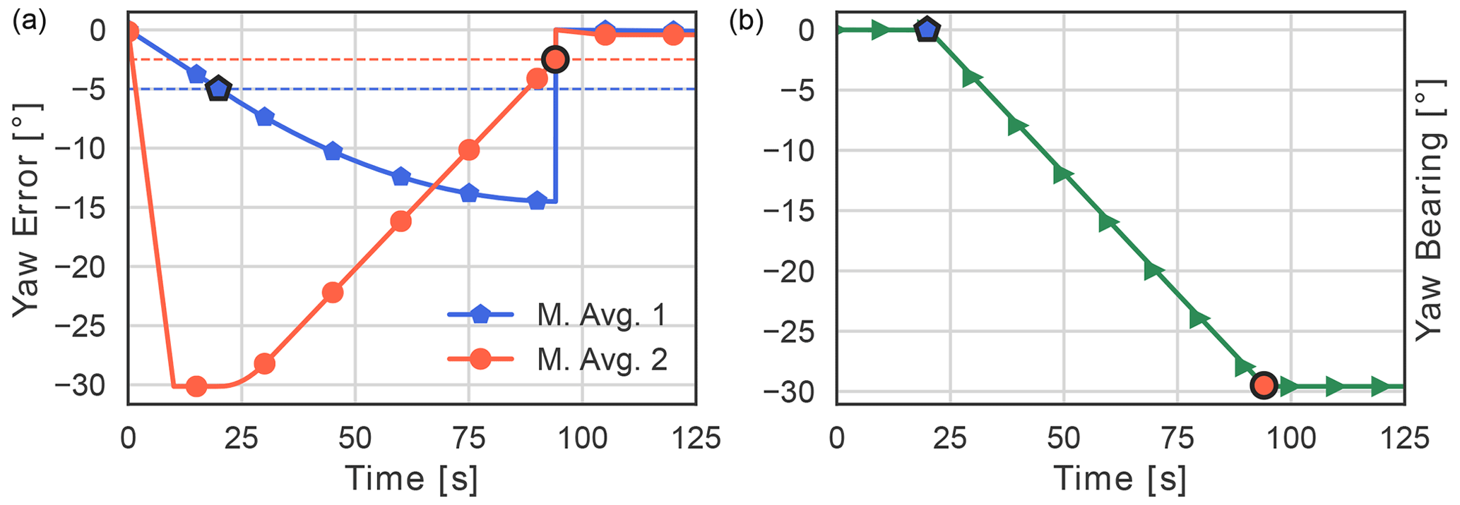
Figure 4 (a) Yaw error as a function of time for start moving average 1 (blue) and stop moving average 2 (red). The dashed blue line shows the start threshold, and the dashed red line shows the stop threshold. (b) Yaw-bearing angle as a function of time.

Figure 4 illustrates an idealized example of the yaw controller action, where the nacelle is initially offset 30^∘ with respect to the mean wind direction. The stop moving average β(t) (red line), with a time window of 10 s, responds much faster to a change in yawing error compared to the start moving average α(t) (blue line) with a window length of 120 s. The threshold θ_t is set to 5^∘, and it can be observed how the wind turbine starts yawing once α(t) exceeds the threshold (right blue marker). The turbine will continue yawing until β(t) (red line) is below θ_s (right red marker), where the instantaneous yaw error is 0.2^∘.

Although a more elaborate study regarding yaw control should be considered, the simple long/short time-averaging approach is chosen here in order not to trigger a yaw action too early (hence 120 s averaging window for the start trigger) while avoiding overshooting after a zero yaw error has been reached (using the 10 s averaging window for the stop trigger).

The yaw mechanism is modeled as a second-order dynamical system with a frequency of 5 Hz and a damping ratio of 0.7. There is no limit on the maximum and minimum yaw angle, allowing a full rotation of the system. It is possible to constrain the response of the second-order model in velocity and acceleration. A typical yaw sweep sequence, yawing 360^∘, lasts around 15 min, which leads to a yaw rate of approximately 0.4^∘ s⁻¹. The proposed basic yaw controller can be replaced with a proportional integral derivative (PID) controller, in which the objective signal is the yaw angle and not the rate of change or velocity of the yaw mechanism.

5 Simulation results

This section contains the results from the HAWC2 simulations. The simulations consist of 3219 points on the 50-year joint gust variable surface with different rise times, amplitudes, and direction changes. The gust surface has been sliced to limit the presentation of simulation results to relevant ranges. The simulation results are shown for a rise-time range of 4–400 s, where the lower rise-time threshold for this range is chosen from considerations of the shortest possible fluctuation turnover time for which the wind field can be considered coherent across the rotor of the DTU 10 MW wind turbine. Further, when considering curves with the same Δt on the 3D gust variable surface, only higher values of the combination of Δθ and Δu are shown for the simulation results (values closest to the origin in Fig. 3 are filtered out).

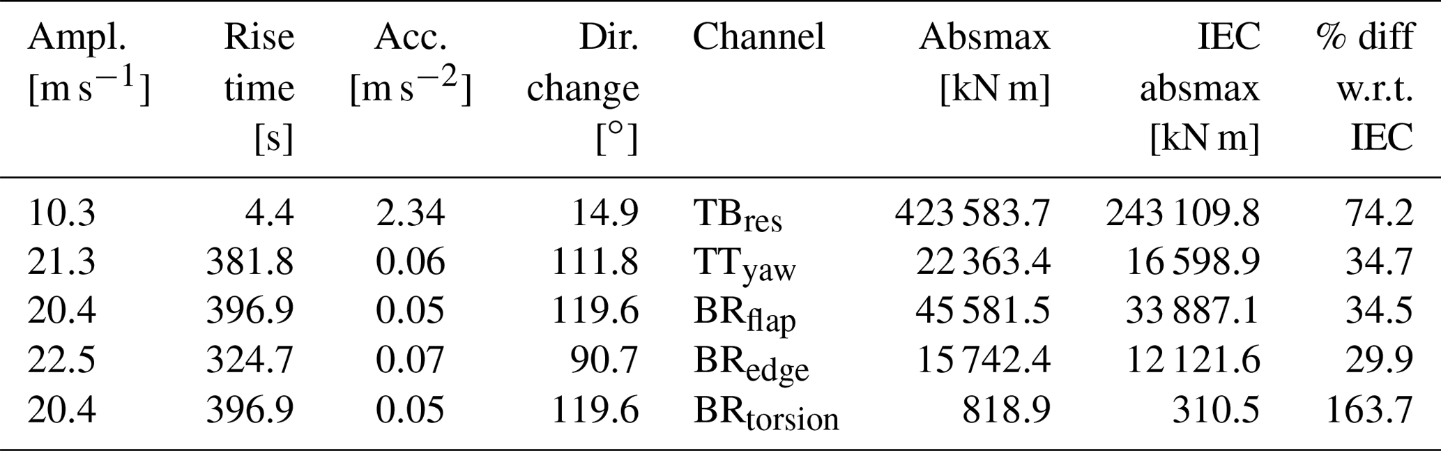
Table 2 Absolute maxima of a selection of load channels with yaw control for gusts starting at 10 m s⁻¹. The IEC absmax (absolute maximum responses) column refers to the IEC DLC1.4 gust case with a rise time of 10 s, amplitude of 15 m s⁻¹, and a directional change of 72^∘.

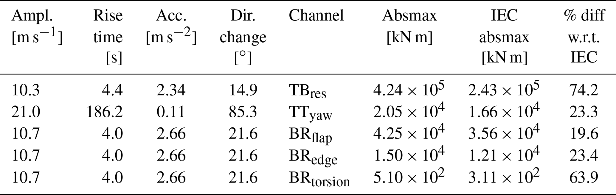
We have simulated the IEC ECD coherent gust for comparison. All simulations have been performed both with and without yaw control, and all gust simulations, including the IEC simulation, start from 10 m s⁻¹. We discuss the implication of using a yaw controller and give an overview of all the simulated gusts and corresponding load maxima. HAWC2 provides output from many different load channels, but here we select a few for further load analysis: the tower-top yaw moment (TT_yaw), blade root flap moment (BR_flap), blade root edgewise moment (BR_edge), blade root torsion (BR_torsion), the tower-bottom fore–aft moment (TB_FA), and the tower-base side–side moment (TB_SS). We further estimate the tower-bottom resultant bending moment (TB_res), defined as ${\mathrm{TB}}_{\mathrm{res}}=\sqrt{{\mathrm{TB}}_{\mathrm{FA}}^{\mathrm{2}}+{\mathrm{TB}}_{\mathrm{SS}}^{\mathrm{2}}}$. The tower-base resultant bending moment provides a clear presentation of the total magnitude of the tower-bottom loading with and without yawing.

5.1 Load response on the 3D gust surface

In this section we focus on the load simulations that were performed with the yaw controller, as we believe that these simulations best represent the load response of a real operating wind turbine.

Figures 5 and 6 give a global overview of the TB_res, TT_yaw, BR_flap, and BR_edge loads. The color indicates the absolute maximum load response of each simulation, which is shown as a dot on the surface. Due to the complexity of the considered 3D gust domain, two alternative views are given to illustrate the response: for Fig. 5 the 3D gust surface is used, while for Fig. 6 the gust amplitude and rise-time axes are collapsed into a gust acceleration dimension (amplitude divided by rise time), and the gust acceleration is plotted on a logarithmic scale.

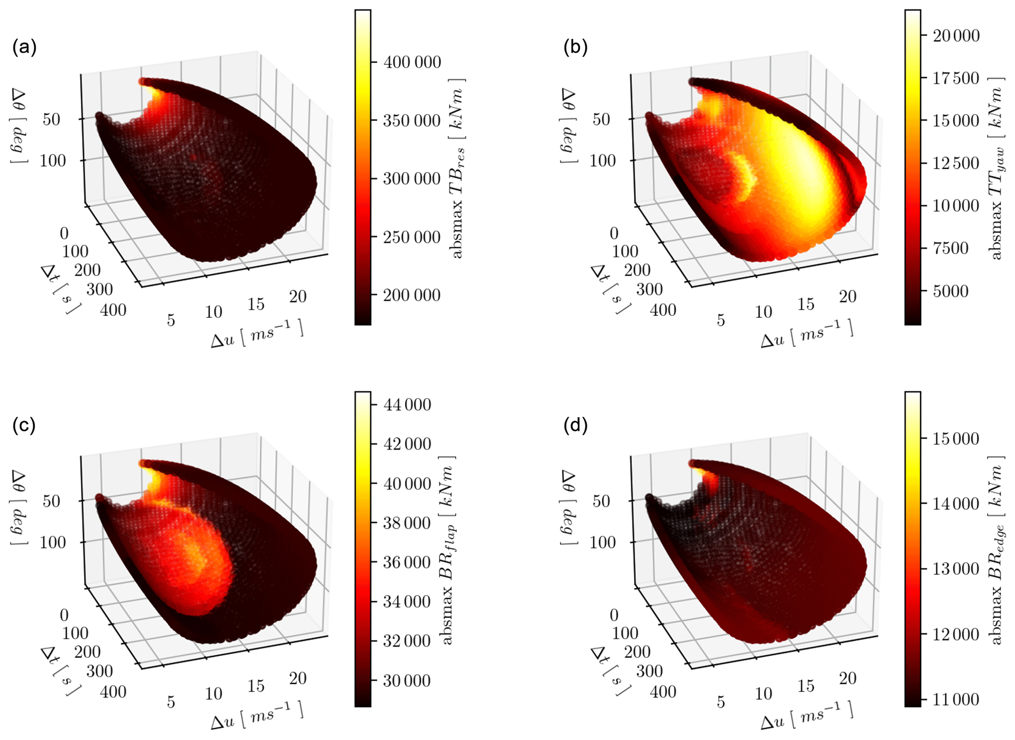
Figure 5 Simulation results with yaw control. The absolute maximum responses are shown with the color scale on the 3D gust variable surface of rise time, amplitude, and direction change. The relevant channel is indicated on the right of the color bar legend: (a) tower-bottom resultant moment, (b) tower-top yawing moment, (c) blade root flap moment, and (d) blade root edge moment.

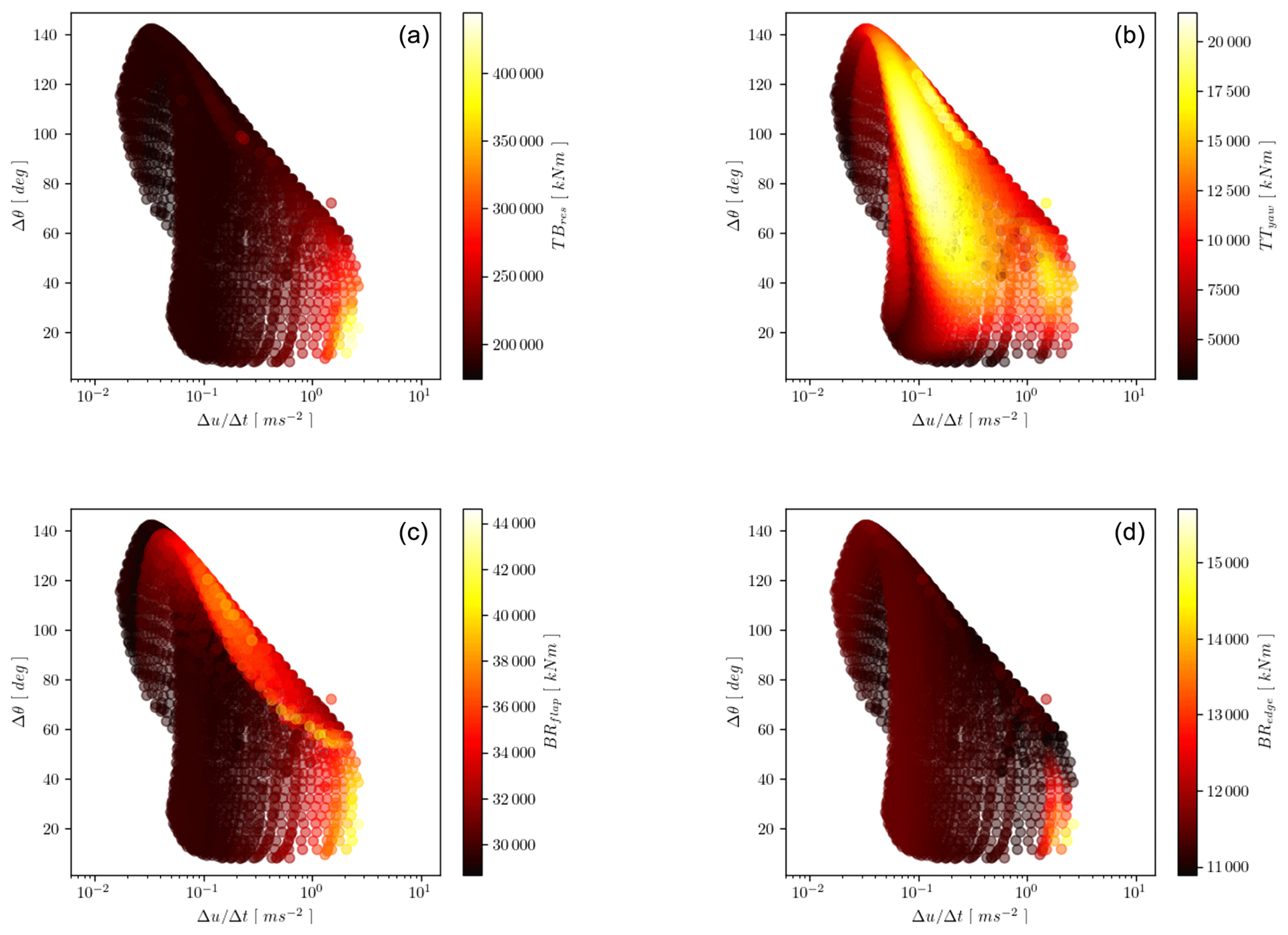
Figure 6 Simulation results with yaw control. The absolute maximum responses are shown with the color scale on the 2D gust variable domain of acceleration and direction change. Notice the IEC ECD gust in all panels is the single outlier. The relevant channel is indicated on the right of the color bar legend: (a) tower-bottom resultant moment, (b) tower-top yawing moment, (c) blade root flap moment, and (d) blade root edge moment.

In Fig. 5 a bright area (indicating the highest loads) for the tower-base and blade root bending moments can be seen. This area corresponds to gusts with small direction changes, short rise times, and relatively modest amplitudes. This is the area for which the absolute maxima of the loads occur, as can also be seen in Table 2. In Fig. 6 this area of highest blade root and tower-base loads is seen for the highest gust accelerations. Further we notice in the highest-gust-acceleration area for the tower-base and blade root edge loads that, for increasing direction change, the max load responses decrease. These load channels are strongly connected with the rotor thrust, which decreases when moderate direction change is introduced.

The blade root flapwise moments also show a circular shape on the surface with moderately high load responses for a large range of the gust variables on the surface (Fig. 5). For this area of the gust surface the direction change is large, and significant yaw errors occur, as the yaw controller reacts more slowly than the direction change in the gusts. It has been verified from the simulations in this area that the rotor speed drops to the minimum after the gust passage due to the high yaw errors (approaching 90^∘). After the gust passage the yaw controller starts to align the turbine again with the wind, which is now well above rated wind speed. The peak blade root bending moments occur around the time when the pitch controller becomes active again to reduce the rapidly increasing aerodynamic thrust and power due to the decreasing yaw angle.

For the tower-top yawing moment a large area (on the right of the 3D gust domain) with high loading corresponds to gusts with high amplitudes, wide range of high rise times, and large changes in direction. The yaw controller is active when the absolute highest tower-top yaw moments occur in the simulations, and the shape of the high-load area is strongly influenced by the current implementation of the yaw controller.

5.2 Comparison with the IEC ECD

The absolute maxima of the response of selected load channels over the considered gust surface are compared with the IEC ECD definition in Table 2. When looking at the blade and tower loading, it is observed that the IEC ECD gust is not conservative and that especially gusts with a lower amplitude and shorter rise time (compared to the IEC ECD) impose a tougher loading condition. Further, it can be noted that all extreme loads for tower-base and blade root bending moments occur for very similar gusts: amplitude of 10.3 or 10.7 m s⁻¹ and with rise times between 4.0 and 4.4 s. Note that for these short gusts one could also consider the initial azimuth position of the rotor to further assure the most critical condition is selected. The tower-top torsional loading (in yawing direction) is different compared to the other channels. The maximum for the TT_yaw occurs for a gust with long rise time, high amplitude, and large direction change.

The difference between what drives the tower-top yawing moment and the tower-base resultant moments is illustrated in Fig. 7. The magnitude of the load is given on the ordinate (y axis), and the gust acceleration is plotted on the abscissa (x axis). The colors mark the magnitude of the direction change in the gust, and the IEC ECD load case is indicated with a white cross (and further marked with a dashed horizontal line). We see that the tower-base loads are driven by the gust acceleration, with almost a linear relationship between gust acceleration and the load response (for similar direction change). It can also be noticed that for comparable gust accelerations the tower-base resultant loads are higher when the direction change is small. The gust acceleration influences the tower-top yawing moments to a lesser extent. The absolute maxima occur for very slow gusts with very large direction changes.

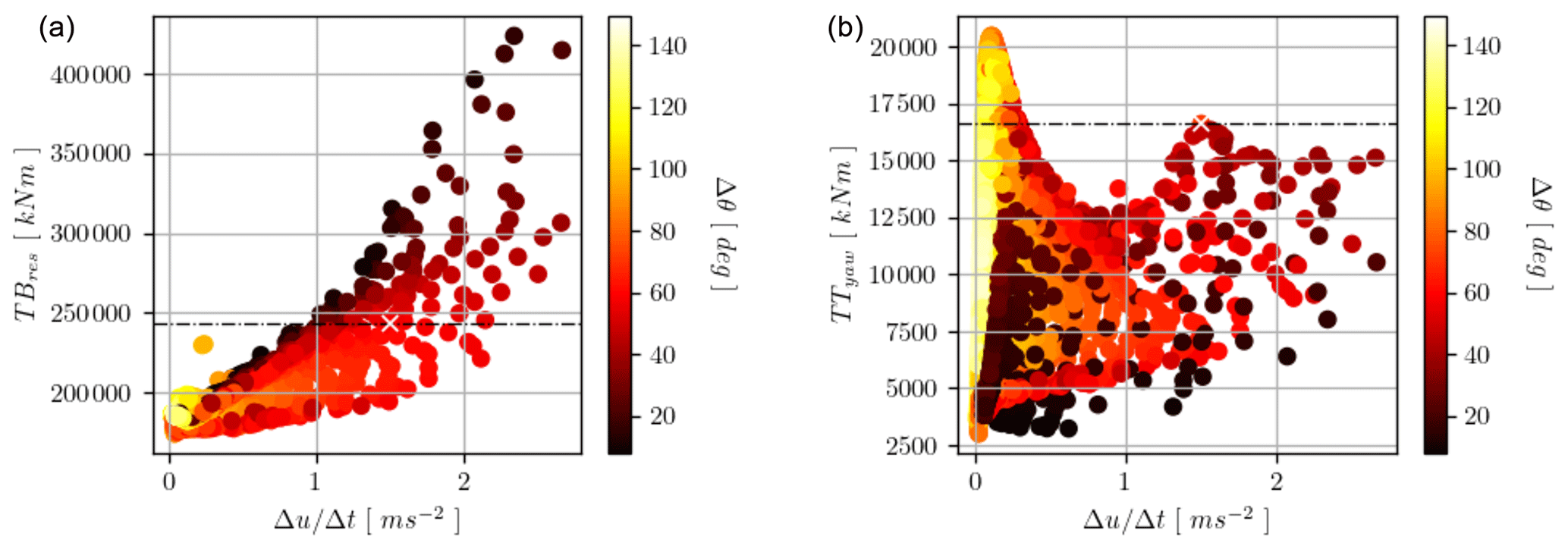
Figure 7 Simulations with yaw control. (a) Tower-base resultant moment as a function of gust acceleration. The colors of the markers refer to the gust directional change in degrees. (b) Tower-top yawing moment as a function of gust acceleration. The marker colors refer to the gust direction change in degrees. The IEC ECD case is marked with a white cross, and its value on the y axis is indicated with the dashed horizontal line.

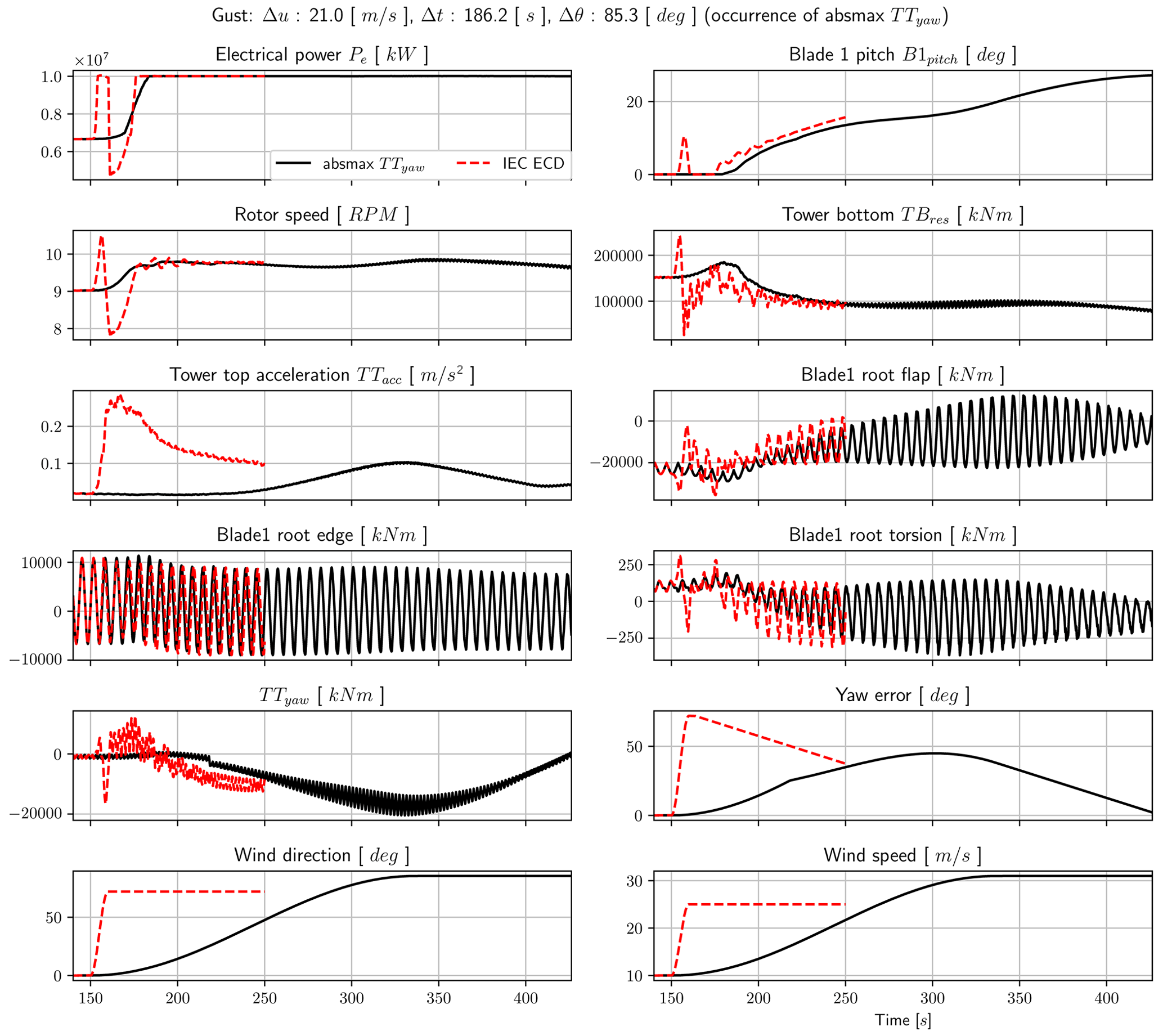
An example time series of the gust resulting in the highest tower-bottom resultant load and tower-top acceleration is compared with the IEC ECD gust in Fig. A1 in Appendix A. Additionally, the gust resulting in the highest tower-top yawing moment compared with the IEC ECD gust is shown in Fig. A2.

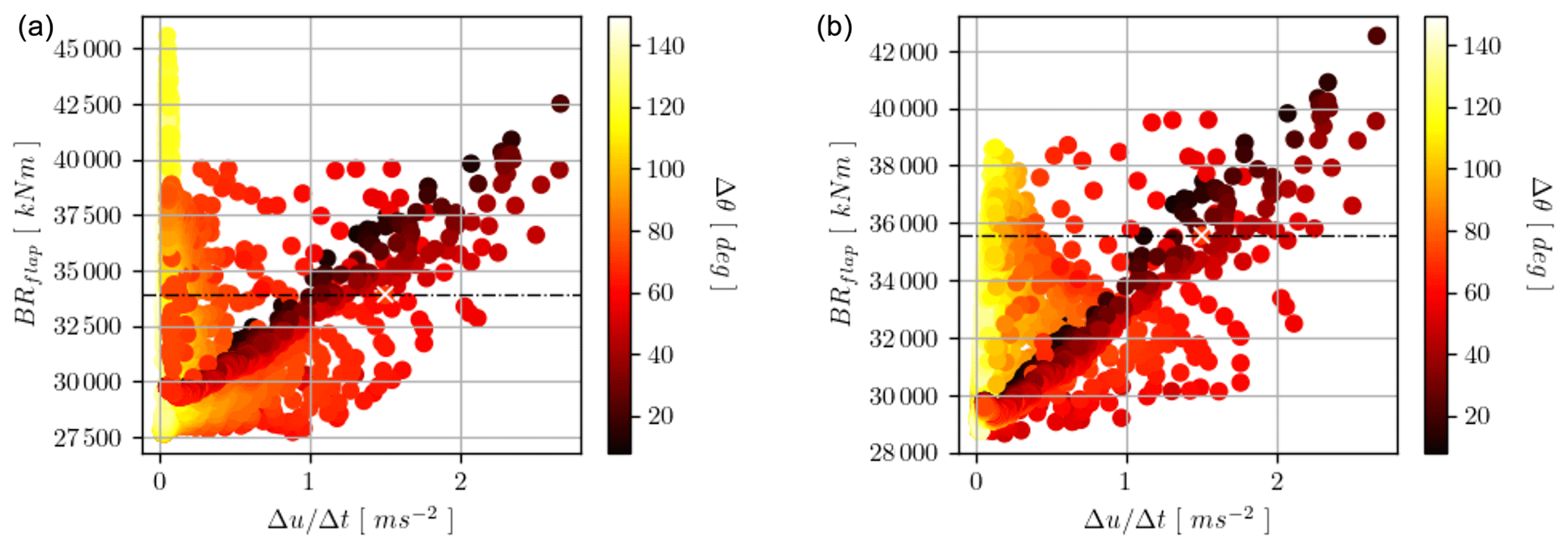
Figure 8 Simulations without yaw control (a) and with yaw control (b). Blade root flapwise loads as a function of gust acceleration. The colors of the markers refer to the gust directional change in degrees. The IEC ECD case is marked with a white cross, and its value on the y axis is indicated with the dashed horizontal line.

Table 3 Absolute maxima of a selection of load channels without yaw control for gusts starting at 10 m s⁻¹. The IEC absmax column refers to the IEC DLC1.4 gust case with a rise time of 10 s, amplitude of 15 m s⁻¹, and a directional change of 72^∘.

5.3 The effect of the yaw controller

The simulations on the gust variable surface were performed both with and without the yaw controller. This was done to investigate the differences in load response between the two simulation sets. Table 3 shows the absolute maxima from a selection of load channels from the HAWC2 simulations that were run without a yaw controller. When comparing the results shown in Tables 2 and 3, it can be seen that the absolute maximum loads are all reduced by including the yaw controller.

In Fig. 8 the absolute maximum of the blade root flapwise bending moment BR_flap is considered. In the left panel we see the results for the simulations that were run without the yaw controller and in the right panel the results that were run with the yaw controller. For this load channel there is a clear dependency on the presence of a yaw controller, and we see that the absolute maximum loads are reduced by including yaw control. This reduction is for gusts with a long rise time.

6 Discussion

In this analysis we chose to extrapolate the multivariate distribution model with a relatively new method, namely the ISORM. Although the IFORM is recommended in the IEC standard, it has been shown to underestimate the probability behind the surface of considered design variables (Chai and Leira, 2018; Dimitrov, 2020). This choice should therefore lead to more accurate values of the 50-year events. It should be noted that using the ISORM instead of the IFORM results in a more conservative gust variable surface and a larger or more extreme variable surface.

According to the probabilistic gust model derived in this analysis, the IEC ECD gust is conservative. That is, with the combination of coherent gust variables, the IEC gust is more extreme and falls outside the 3D gust parameter surface. By increasing the return period to 460 years, the IEC gust is matched on the surface of the probabilistic gust surface. Though we did find that the IEC gust is more conservative with regards to the gust variables, it is interesting to see that higher loads can be reached with simulations from the probabilistic gust model. By including variability in the gust parameters, we were able to identify critical regions on the gust parameter surface that lead to loads that are significantly higher (up to 74 %) than those that come from the simulation of the IEC ECD gust.

The current analysis is based on data from a single site and is therefore likely to be site specific. Although previous studies on coherent structures (e.g., Hannesdóttir and Kelly, 2019; Belušić and Mahrt, 2012) imply that these kinds of events occur at many different sites, the current probabilistic gust model is based on one site only. Future work could be to derive a more general gust model that would represent any site or could be made site specific with IEC wind turbine class parameters.

We also note that all the results shown in Figs. 5 and 6 are highly dependent on the DTU 10 MW wind turbine model, the basic DTU Wind Energy controller, and the yaw controller used in the simulations. We expect that commercial controllers designed by wind turbine manufacturers are more advanced and may react to extreme events in a different way. It would be possible to change the overall picture of the load results by tuning or optimizing the controller to handle gust cases with extreme gust accelerations, but that is outside the scope of the current study.

Although not discussed in the current work, the aerodynamic response under yawed inflow conditions is another topic of concern since the accuracy of the blade element momentum method (BEM) may decrease as the yaw error increases, and generally such results should be considered carefully. However, the BEM implementation used in HAWC2 employs a yawed inflow correction and assumes non-constant induction across an angular ring element (see Madsen et al., 2020).

7 Conclusions

In this work observations of coherent gusts are used to obtain an environmental surface with a 50-year return period with the Nataf distribution model. The surface is a 3D gust variable space of rise time, amplitude, and direction change. There is a large variability within the modeled gust variables, where the direction change and amplitude may exceed the ECD values, though in these cases with a considerably longer rise time. For modeled gusts with 10 s rise time, the maximum amplitude is 8.3 m s⁻¹ and the maximum direction change is 35.3^∘.

The modeled gust variable surface can match the values of the IEC ECD gust parameters by using a return period of approximately 460 years.

We choose 3219 points on the surface to simulate for wind turbine response, where the simulations are performed with and without a yaw controller that is specially developed in this study.

The effect of the yaw controller is seen for the modeled gusts, where we see that the absolute maximum of all the considered load responses is lowered by including the yaw controller, especially for gusts with a relatively long rise time in which the blade root torsion and flapwise bending moments are significantly reduced when the wind turbine yaws.

From the comparison of the modeled gusts and the IEC ECD, we find that, even though the modeled gusts are not as severe in terms of gust variables, the difference in observed extreme loads is higher. From the considered load component channels, the largest difference is seen for the tower-base resultant moment, which is 74.2 % higher for the modeled gust compared with the IEC gust. Similarly, the blade root torsion load is 63.9 % higher for the modeled gust, and the blade root flapwise, blade root edgewise, and tower-top yaw moments are around 20 % higher than the simulated ECD gust. The maximum loads for TB_res, BR_flap, BR_edge, BR_torsion, and TT_acc are observed for the modeled gusts with short rise times, between 4.0 and 4.4 s, and low direction change, between 14.9 and 21.6^∘, while the maximum load for the TT_yaw is observed from a modeled gust with a longer rise time of 186.2 s and a large direction change of 85.3^∘.

In the current work we have used the basic DTU Wind Energy controller with the specific DTU 10 MW tuning parameters. We acknowledge that our simulation results depend on the general response of the controller. While it is out of the scope of the current study, an improved controller (tuning) could change the response significantly, and follow-up work could consider this aspect. Similarly, an improved tuning of the simple yaw controller could be performed to establish in more detail how yaw control can affect the loads and how much inertial loading a yawing and rotating turbine can experience.

Appendix A: Time series of the extreme cases for a selection of channels

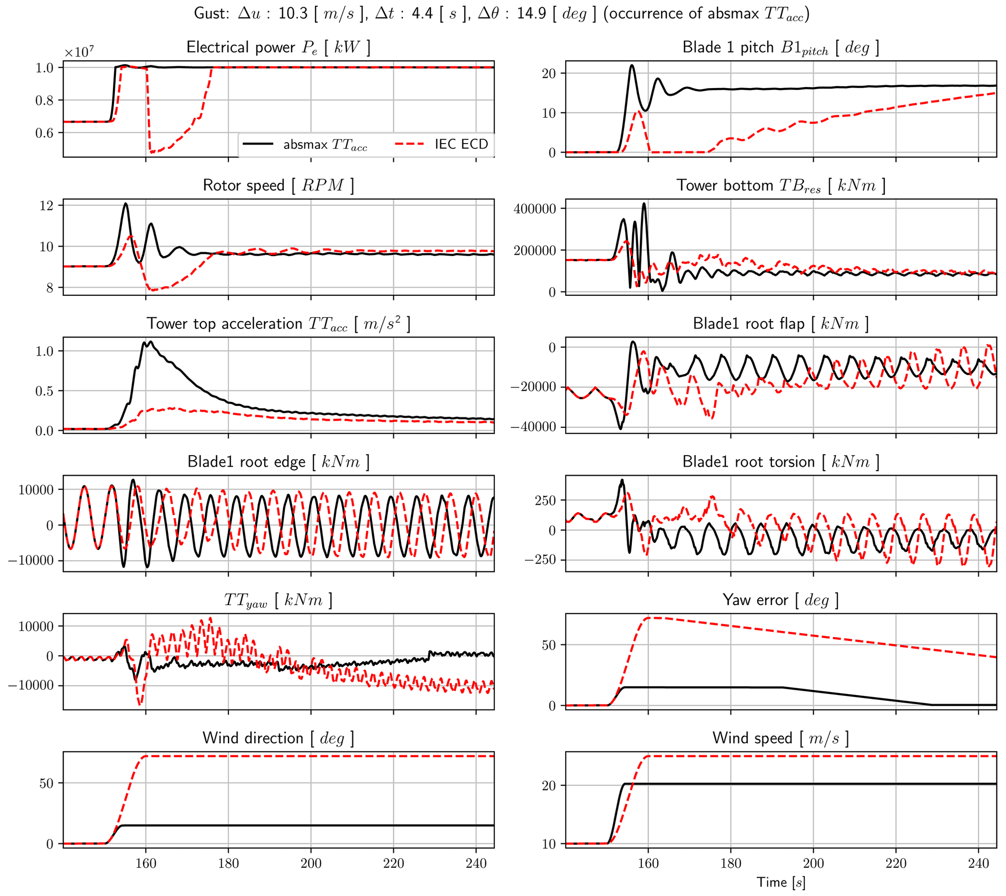
Figure A1 Gust for which the tower-bottom resultant bending moment TB_res and the tower-top acceleration TT_acc have the absolute maximum (see also Table 2). Note that the label is only shown in the upper-left panel (solid line for the gust case as indicated in the panel title and dotted line for the IEC ECD gust).

Figure A2 Gust for which the tower-top yawing moment TT_yaw has the absolute maximum (see also Table 2). Note that the label is only shown in the upper-left figure (solid line for the gust case as indicated in the panel title and dotted line for the IEC ECD gust).