the Creative Commons Attribution 4.0 License.
the Creative Commons Attribution 4.0 License.
 | 08 Mar 2023
Cyclic overlay model of p–y curves for laterally loaded monopiles in cohesionless soil
Junnan Song
Martin Achmus
The bearing behaviour of large-diameter monopile foundations for offshore wind turbines under lateral cyclic loads in cohesionless soil is an issue of ongoing research. In practice, mostly the p–y approach is applied in the design of monopiles. Recently, modifications of the original p–y approach for monotonic loading stated in the API regulations have been proposed to account for the special bearing behaviour of large-diameter piles with small length-to-diameter ratios. However, cyclic loading for horizontally loaded piles predominates the serviceability of the offshore wind converters, and the actual number of load cycles cannot be considered by the cyclic p–y approach of the API regulations. This research therefore focuses on the effects of cyclic loading on the p–y curves along the pile shaft and aims to develop a cyclic overlay model to determine the cyclic p–y curves valid for a lateral load with a given number of load cycles. A stiffness degradation method (SDM) is applied in a three-dimensional finite element model to determine the effect of the cyclic loading by degrading the secant soil stiffness according to the magnitude of cyclic loading and number of load cycles based on the results of cyclic triaxial tests. Thereby, the numerical simulation results are used to develop a cyclic overlay model, i.e. an analytical approach to adapt the monotonic (or static) p–y curve to the number of load cycles. The new model is applied to a reference system and compared to the API approach for cyclic loads.
- Article
(5475 KB) - Full-text XML
- BibTeX
- EndNote


The conversion of energy supply to the extensive utilization of renewable energies can only be realized by further expansion of offshore wind energy. In this regard, it is crucial to minimize the costs for offshore wind energy exploitation. Significant cost savings are possible by optimizing the foundation elements of offshore wind energy converters.
In the last years, the monopile foundation, consisting of a circular steel pipe of very large diameter (Fig. 1), was proven to be an economic and robust foundation solution for water depths of up to around 40 m. For the time being, projects are being realized with monopiles of up to 10 m outer diameter. However, there are still basic uncertainties in the design of such monopiles. In practice, usually the p–y method is applied in the calculation of the monopile behaviour. This is a special subgrade reaction method, which utilizes nonlinear and depth-dependent spring characteristics, the p–y curves. Here p is the resultant soil resistance (horizontal bedding stress times pile diameter) at a certain depth, and y is the corresponding horizontal pile displacement. In offshore guidelines, for example, API (2014) approaches to derive p–y curves dependent on the parameters of the present soil are given. For piles in sand, the only parameters required are the buoyant unit weight γ′ and the angle of internal friction ϕ′. However, several investigations in recent years have shown that these approaches, which have been calibrated by field test results of slender, flexible piles, cannot be used without modification for the large-diameter and almost rigid monopiles. This applies both to the p–y approaches for static (monotonic) and cyclic loads.
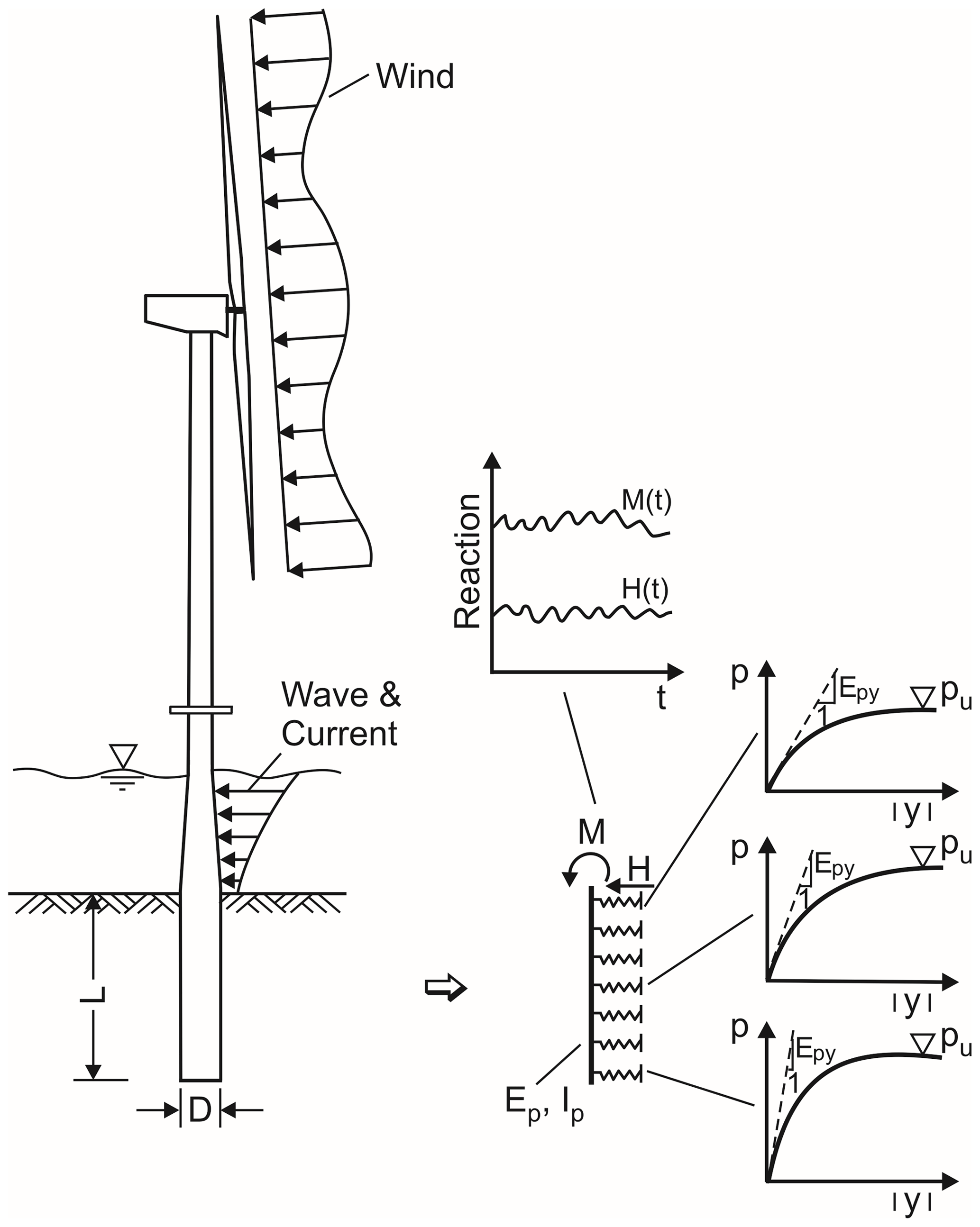
Figure 1Monopile foundation of an offshore wind energy converter and p–y method used in design (schematic).
In the classic approach for piles in sand according to API (2014), a tangent hyperbolic function is used to describe the dependence of bedding resistance p on horizontal displacement y at a certain depth below sea bottom z:
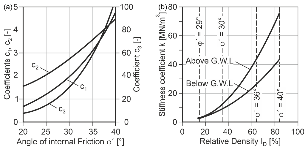
Here pu is the theoretical maximum value of bedding resistance, which is basically the passive earth pressure times pile diameter D. This value is calculated from Eq. (2) as a minimum of two values for shallow and deep failure modes pus and pud, which depend on buoyant unit weight γ′ and three coefficients C1, C2 and C3 correlated with the angle of internal friction ϕ' (Fig. 2 left).
The k value in Eq. (1) is a stiffness parameter and is also given in API (2014) dependent on the angle of internal friction (Fig. 2 right).
For the factor A in Eq. (1), the API approach distinguishes static and cyclic loading conditions. For static loading, applies, whereas for cycling loading the constant factor (independent of depth) Acyc=0.9 shall be used.
Several investigations have shown that for large-diameter piles the pile–soil stiffness obtained with the static p–y method is overestimated under extreme loads and underestimated under smaller operational loads (cf. e.g. Thieken et al., 2015a). Therefore, new static p–y approaches for monopiles in sand have been proposed in recent years. Sørensen (2012) replaced the k value of the API guidelines by a k value depending on depth z, the soil's oedometric stiffness Es and the pile diameter D, which for large-diameter piles leads to greater displacements under service loads than the API approach. Kallehave et al. (2012) also suggested a modified initial stiffness formulation, but their target was to avoid an underestimation of stiffness under small operational loads, which is usually applied for the determination of the natural frequency of the whole structure. Here, the parameter k is formulated dependent on depth z and pile diameter D. This modified p–y formulation results in a considerably “stiffer” behaviour than the API formulation. Thieken et al. (2015b) proposed a more sophisticated p–y curve approach, in which also the soil's greater stiffness for small strains is considered and which accounts for the effect of the pile deformation on the p–y curves by an iterative procedure. They showed that this approach gives reasonable results both for small operational and large service loads. Recently, Byrne et al. (2017) also proposed a new p–y approach especially developed for monopiles in sand soil (see also Byrne et al., 2015; Burd et al., 2020). Herein, besides p–y springs, also rotational springs and a pile tip spring are introduced to the beam-spring model. However, the spring characteristics are to be determined by calibration with a numerical model, which makes the approach not straightaway applicable to a certain system.
Cyclic loading of a pile can lead to both an increase of pile deformation with the number of load cycles and a reduction of the pile capacity, whereby in sand soils the effect on deformation usually dominates the design. Cyclic loading effects are considered in design by applying cyclic p–y curves in the calculation. As shown above, in the approach of API (2014) cyclic loading is considered by a reduction of the parameter A and hence the bedding resistance p down to a depth of z= 2.625 D. However, since the parameter A also affects the argument of the tanh function, also displacements are affected, which means that the API consideration for cyclic loads is a mixture of p- and y-multiplier methods. The approach is based on field tests, in which for the determination of cyclic loading effects only limited load cycle numbers (at maximum around 200) were realized (Cox et al., 1974). It is generally assumed that the approach represents the pile behaviour due to around 100 load cycles.
Apart from the fact that the cyclic API approach is not validated for large-diameter monopiles, the consideration of just one cyclic p–y curve valid for 100 load cycles is not sufficient for the design of piles for offshore wind foundations. These foundations are subject to intense cyclic loading induced by wind and wave loading. The design checks for cyclically accumulated deformations and in particular rotations of the foundation structure is quite important for wind energy structures. In most wind farm projects, a maximum permanent rotation of the tower of 0.5∘ is required. Thus, an accurate prediction of the accumulated pile rotation of the monopile to be expected over the whole lifetime of the structure is necessary. This means that the deformations must be calculated under consideration of the actual number of load cycles.
Dührkop (2009) conducted model tests with almost rigid monopiles in sand under cyclic loading. Based on the results, he proposed a modification of Eq. (1) for the case of cyclic loading as follows:
with .
The factor rA is dependent on the number of load cycles. With rA= 1, the API approach for monotonic loading and with rA= 0.3 for cyclic loading is obtained. Thus, rA= 0.3 can be used for a load cycle number of N= 100. For greater load cycle numbers, rA decreases. For N > 105, rA shall be set to zero (Dührkop, 2009). With this approach, the monopile deflection can be calculated dependent on the actual number of load cycles. However, the given Acyc function is valid only for the model test boundary conditions realized by Dührkop. For a certain system with different boundary conditions, model tests or numerical investigations are necessary.
Besides from local approaches modifying the p–y curves, also global approaches predicting the increase of pile head deflection or rotation can be applied. In general, the increase of head deflection due to one-way loading with full unloading can be described by the following equation:
Here yN and y1 are the horizontal pile head deflections after N load cycles and after 1 load cycle (monotonic loading), respectively. fN (N) is a function which describes the increase of deflections with the number of load cycles. As long as the cyclic load amplitude is well below the ultimate pile capacity, sedation behaviour can be expected, which means that the deflection rate decreases with increasing number of load cycles. The most common functions of displacement of structures under cyclic loading that are found in the literature are of the exponential type such as Eq. (5) (e.g. Little and Briaud, 1988) and of logarithmic type such as Eq. (6) (e.g. Hettler, 1981):
Here m and t are empirical accumulation parameters. Assuming that these parameters are constants, Eqs. (5) and (6) imply that the function of load cycle number is independent of the load amplitude.
A few investigations regarding the above accumulation parameters exist. In addition to the above-mentioned works, Lin and Liao (1999) and Long and Vanneste (1994) should be mentioned. However, it is not clear how pile geometry (in particular, pile rigidity) and soil conditions affect the accumulation parameters. Based on model tests, LeBlanc et al. (2010) showed that the rate of deformation accumulation also depends on the load level, i.e. the ratio of maximum cyclic load to the ultimate pile capacity. In contrast, model test results of Peralta and Achmus (2010) did not show a significant effect of the load level.
For practical design, a simple-to-use approach for the derivation of cyclic p–y curves would be highly desirable, which just modifies a chosen static p–y curve by p or y multipliers depending on the number of load cycles and other relevant parameters. Such an overlay model describes just the change of static p–y curves with increasing load cycle numbers and could be applied to arbitrary static p–y curve approaches.
A calculation approach termed “stiffness degradation method” (SDM) combining numerical simulations and cyclic triaxial tests has been developed at the Institute for Geotechnical Engineering of Leibniz University Hanover (Achmus et al., 2009). This method allows the calculation of pile deflection lines dependent on the actual number of cycles of a given load and with that also the derivation of p–y curves for a given number of load cycles. This method is applied in the paper at hand for the development of a cyclic p–y overlay model. Therefore, the SDM is briefly described in the following section.
The SDM is described in detail in Kuo (2008) and in other publications, e.g. Achmus et al. (2009) and Kuo et al. (2012), and thus here the method shall be outlined just briefly. A 3-dimensional finite element model is used to calculate the pile deformation behaviour. The soil behaviour under static load is modelled by an elastoplastic material law with the Mohr–Coulomb failure criterion and stress-dependent stiffness. The stiffness modulus, i.e. the oedometric stiffness determined under constrained lateral strain, is defined as follows:
Herein σat= 100 kN m−2 is a reference (atmospheric) stress, σm is the current mean principal stress in the considered soil element, and κ and λ are soil stiffness parameters.
For describing the increase of the plastic strain of soil with the number of load cycles in element tests (cyclic triaxial tests), an approach by Huurman (1996) is used. The decrease of the (secant) stiffness modulus of the soil with the number of cycles can be approximated by the following equation:
Herein N is the number of cycles, b1 and b2 are regression parameters and is the cyclic stress ratio, whereby σ1,cyc is the maximum of the principal stress in a cycle and σ1,f is the main principal stress at failure (in a static test). For each element of the finite element model, from the consideration of the initial stress state and the stress state after applying the horizontal load, a cyclic stress ratio quantifying the intensity of cyclic loading is derived. With the reduced stiffness values obtained from Eq. (8), the system's behaviour under the lateral load is calculated again. The result represents the increased pile deformation after the considered number of cycles. An illustration of the procedure is given in Fig. 3.
For cyclic one-way loading and drained conditions, the SDM allows the evaluation of the pile deformation behaviour under consideration of the site-specific soil conditions as well as the loading conditions and the number of cycles. The application requires the definition of six material parameters accounting for the soil behaviour under static loading, for which comprehensive experiences exist, and two parameters b1 and b2 describing the stiffness degradation under cyclic loading.
The method has been validated by back-calculation of various series of model tests in medium-dense as well as in dense sand (see Albiker, 2016; Albiker and Achmus, 2018). From these back-calculations, it could be concluded that for comparable relative densities of the soil also consistent sets of values for b1 and b2 have to be chosen. Value sets for medium-dense and dense sand were determined by comparison of calculations and experimental measurements, and the ranges of values were also verified by regression values derived from cyclic triaxial tests (Albiker, 2016).
4.1 General
The constitutive law for sand used in the SDM is a simple elastoplastic material law with the Mohr–Coulomb failure criterion and stress-dependent formulated stiffness. Consequently, this constitutive law is also used in the simulations presented here. It was proven that this model yields reasonable results regarding the behaviour of monopiles under horizontal and moment loading (e.g. Achmus et al., 2009). Actually, a high accuracy of the simulation model for static loading is not crucial, since only the differences between static and cyclic pile behaviour are of relevance here. Basically, the overlay model to be developed shall be applicable to any static p–y approach.
The numerical calculation is done for half of the system (Fig. 4) and is divided in several phases.
-
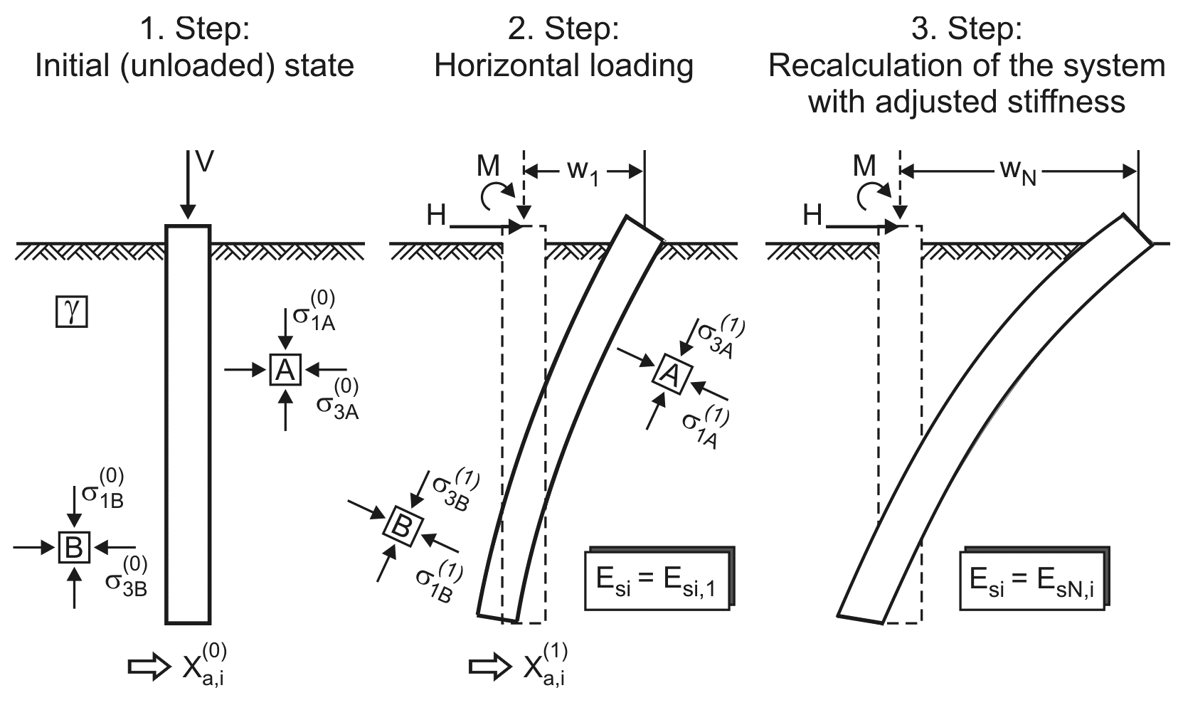
In the first calculation phase, the initial stress state in the soil is generated, considering the coefficient of earth pressure at rest in the determination of horizontal stresses. Based on this initial stress state, the oedometric stiffness modulus of each soil element is calculated from Eq. (7). Afterwards, the soil elements located at the location of the monopile are replaced by steel elements.
-
In the second phase, the horizontal loading on the system is applied incrementally. After each load step, the horizontal stresses acting on the pile are integrated over certain depth sections of the pile in order to determine the p values belonging to the current load for the considered depths. Plotting the p values for different loading steps over the corresponding pile deformations y at the same depth gives the p–y curves for static loading.
-
For the derivation of cyclic p–y curves, the stress conditions in the soil are evaluated after each load step in order to determine the degraded soil stiffness dependent on the considered load cycle number N according to Eq. (8). The numerical simulation is then repeated under consideration of the reduced stiffness until the static load level is again reached. This procedure yields for each point of the static p–y curve a corresponding point of the cyclic p–y curve belonging to the load cycle number N. The calculations presented here were carried out for load cycle numbers of N= 1 (static), 10, 100, 1000 and 10 000.
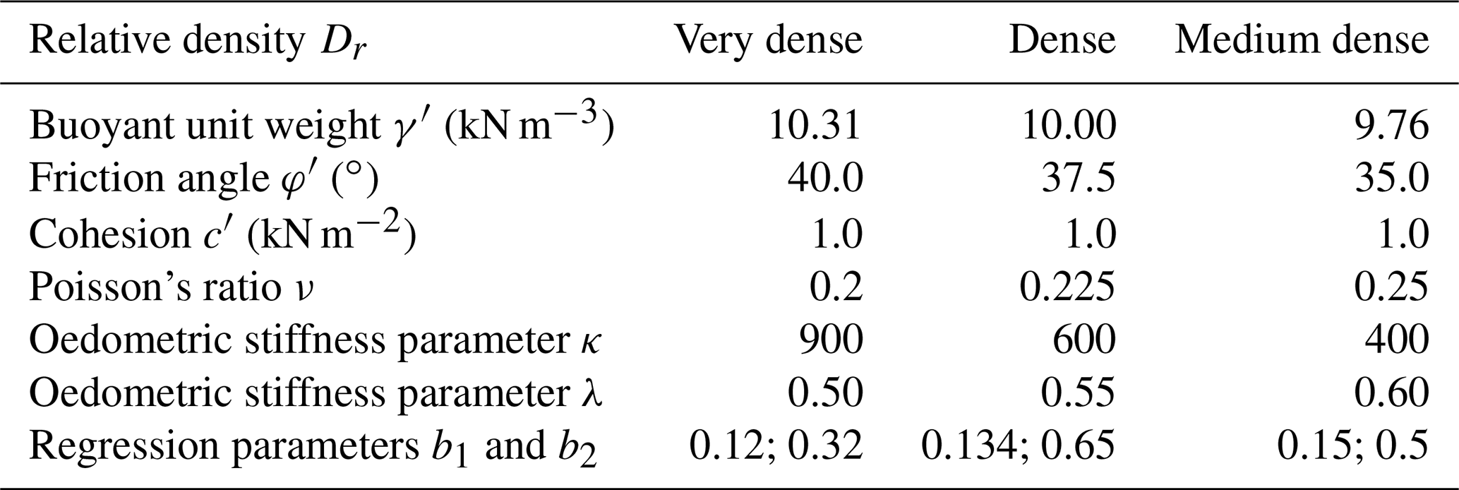
The parameters of the sand used in the numerical simulations are given in Table 1 for three different relative densities. These are typical parameters for sands. The regression parameters b1 and b2 of the SDM model were chosen according to the evaluation of cyclic triaxial tests given in Albiker (2016).
Table 1Material parameters used for sand with three different relative densities.
Generally, p–y curves are dependent on the load conditions (e.g. lever arm, which is the ratio of bending moment and horizontal load) and on the deformation mode (deflection line) of the pile. Therefore, a procedure also applied by Thieken et al. (2015b) was followed, in which at first p–y curves (and here the corresponding overlay model) for purely translatoric displacement of a rigid pile are derived. Afterwards, variable load conditions and hence variable deformation modes are considered in order to derive correction functions accounting for the actual pile deflection line.
4.2 p–y curves for constant deflection – basic overlay model
The basic p–y curves and the basic overlay model apply to a constant horizontal deflection of the pile, which was achieved by assigning identical prescribed displacements to all the pile nodes. With that, the effect of a pile rotation and pile bending is switched off.
The pile diameter was varied between D= 3 and D= 8 m in 1 m steps. The pile length was set to L= 25 m in all calculations. Due to the enforced rigid body motion, wall thickness and pile bending stiffness play no role.
The simulations were conducted with the finite element code Abaqus (Abaqus, 2016) using eight-noded volume elements (C3D8). Only one half of the three-dimensional cylindrical system was modelled, thereby utilizing symmetry conditions. The sufficient size of the model domain and sufficient fineness of the finite element mesh were proven by preceding sensitivity analyses. For instance, the model for the pile with 5 m diameter and a length of 25 m had a width of 100 m (dimension in direction of the horizontal load), a breadth of 50 m and a depth of 50 m. At the edges of the domain, horizontal supports were considered for the nodes in the vertical planes and vertical supports for the nodes in the bottom plane.
Figure 4 shows the distribution of horizontal displacements and horizontal stresses for a monopile with 5 m diameter in very dense sand under static loading (N= 1) as an example. The evaluation of these calculation results yields for each considered depth along the monopile axis one point of the p–y curve.
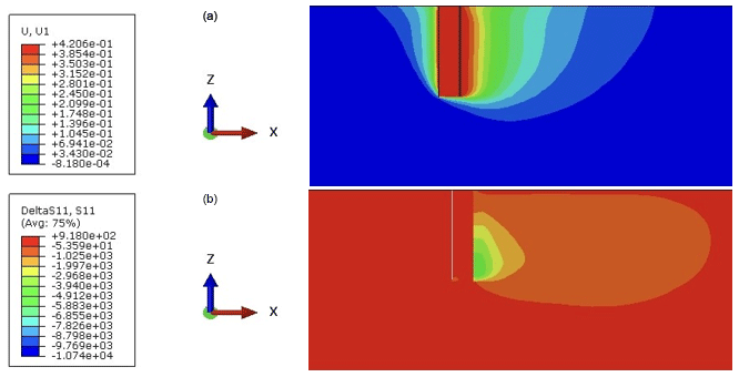
Figure 4Horizontal displacements (a) and stresses (b) for a monopile D= 5 m under static load in very dense sand (N= 1, prescribed pile displacement y= 0.42 m).
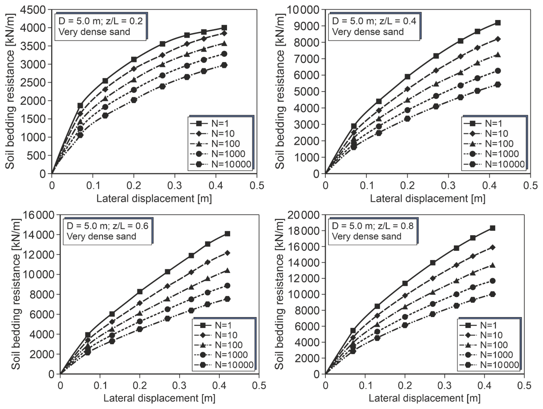
Figure 5 shows the derived p–y curves at four different depths for the pile with D= 5 m in very dense sand. The maximum realized displacement was 0.42 m, which is more than 8 % of the pile diameter. As to be expected, the bedding resistances and thus the spring stiffness increase with increasing depth. Also as expected, cyclic loading leads to greater displacements and thus reduced spring stiffness. It is noteworthy that the relative difference of the cyclic curves to the static curve seems to be quite similar in all depths.
Since the applied SDM method accounts for cyclic effects by a stiffness reduction of the soil, it is deemed logical to try to transfer the static to the cyclic curves by a y multiplier. Figure 6 shows the determined values for the results shown in Figs. 4 and 5. Also regression curves are presented. Evidently, the same function independent of absolute displacement and depth can well approximate the calculation results.
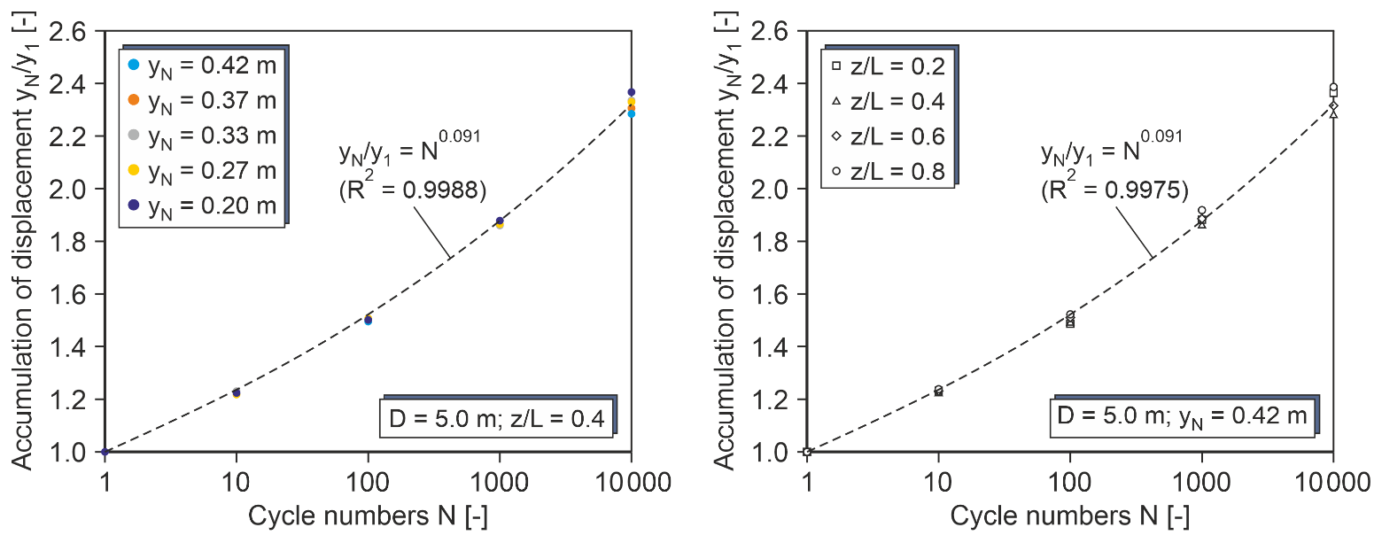
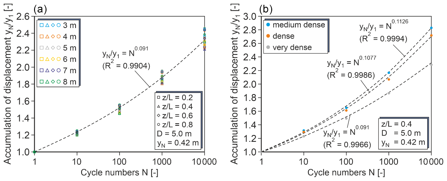
Figure 7y multipliers for variable pile diameters (a) and for different relative densities of the sand (b).
Figure 7 depicts the effects of varying pile diameters and soil relative densities. Figure 7 left shows for varied pile diameter and relative depth the y multiplier determined at a representative point of the respective p–y curve (yN= 0.42 m). Obviously, the same function already presented in Fig. 6 gives a good approximation also for piles of other diameters than 5 m. Eventually, Fig. 7 right shows the calculated bandwidths of y multipliers for varying relative densities of the sand, which were derived in the same manner as described above. A considerable dependence of the y multipliers on relative density can be seen, which was expected because different regression parameters b1 and b2 in the SDM apply for different relative densities. A lower relative density leads to stronger relative accumulation of pile displacements and hence to a stronger cyclic degradation of the p–y curves.
The approach for the derivation of cyclic p–y curves from a given static p–y curve valid for constant lateral displacement of a pile (basic overlay model) can be summarized as follows:
where N denotes cycle numbers of .
Accounting for the internal friction angles ϕ′ of the sands considered in the numerical simulations (cf. Table 1), the exponent A can be expressed by
where φ′ denotes the internal friction angle of sand in [∘] ( 35.0–40.0∘).
4.3 p–y curves for arbitrary loading conditions – advanced overlay model
In the next step, the effects of load eccentricity, pile bending stiffness and normalized pile length shall be considered. Hence, a parametric study was conducted, in which monopiles were loaded by a horizontal force and a bending moment applied at the point of embedment (Fig. 8; the bending moment is the product of horizontal force and considered load eccentricity).
In the following, results for a reference system with a diameter of D= 5 m in very dense sand are presented. A wall thickness of t= 7 cm was assumed, which is a typical value for monopiles of such diameter. Load eccentricities 0, 0.4, 0.6 and 1.0 and normalized pile lengths 5, 6, 7 and 8 were considered. Linear elastic behaviour was assigned to the steel elements of the pile with Young's modulus Epile= 2.1×10⁸ kN m−2 and Poisson's ratio of νpile = 0.3. For the very dense sand, the parameters given in Table 1 were applied.
Figure 9 elucidates exemplarily how correction factors to be applied to the basic overlay model were derived. Depth-dependent p–y curves for varied number of loading cycles were determined for given geometry and loading conditions. The curves were then compared to the curves of the basic overlay model. It was again found that the transfer from the basic curves to the actual curves could be well approximated by application of a y multiplier independent of load level (cf. Fig. 9 right). Hence, a correction factor Ω was defined as follows:
where yactual and ybasic are the pile displacements at a given depth z for the actual pile and load configuration and pile displacement for the same p value according to the basic overlay model.
Figure 9 shows that for the considered depth z= 0.4 L the actual p–y curves are stiffer than the curves determined with the basic overlay model. This means that the correction factors are smaller than unity.

Figure 9Exemplary comparison of p–y curves for constant horizontal displacement (bold lines) and p–y curves for the actual configuration (monopile in very dense sand).
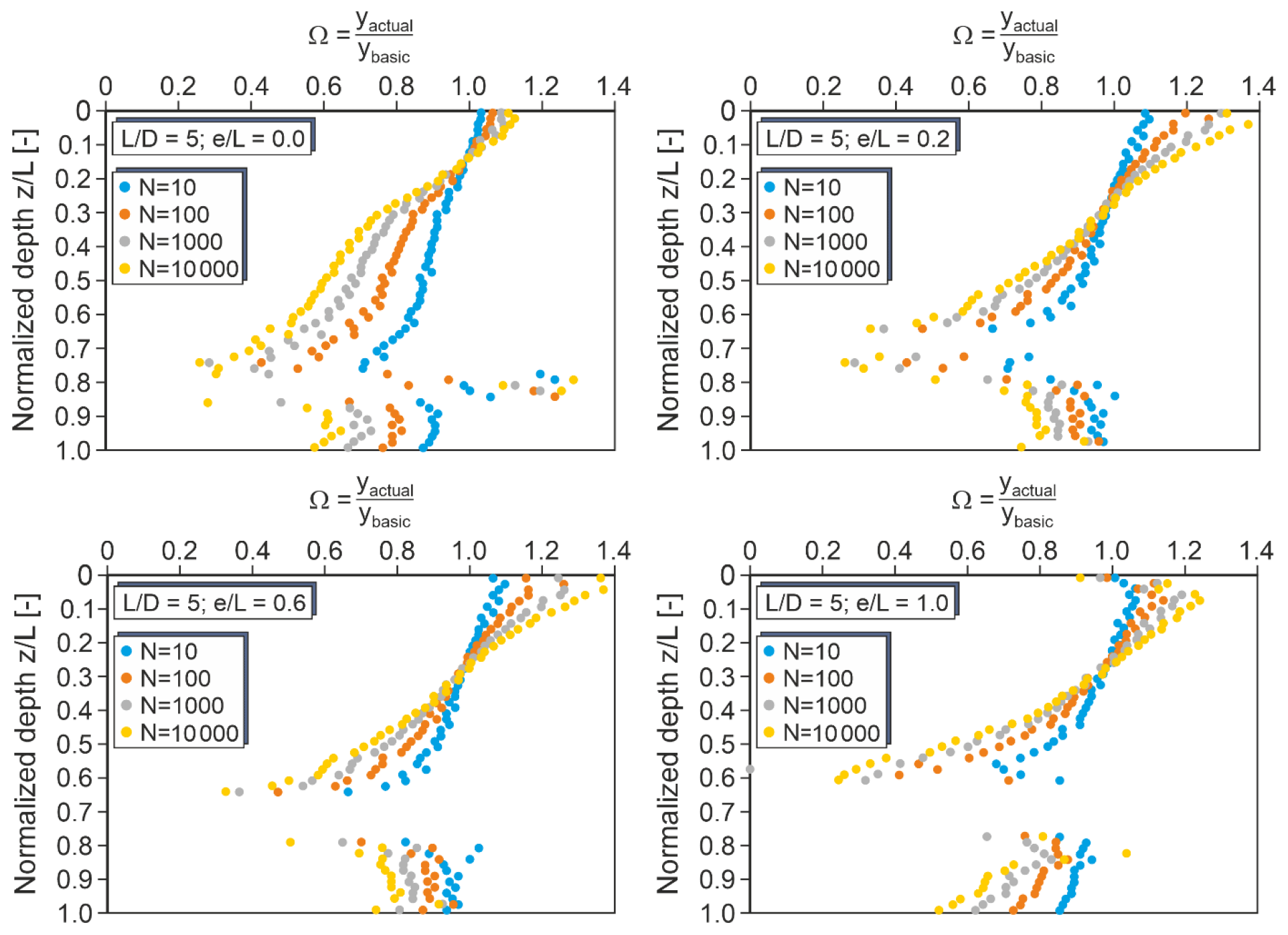
Figure 10Correction factors Ω for monopiles with 5 and different load eccentricities (very dense sand).
The correction factors determined for the system given in Fig. 9 are presented in Fig. 10 (top right), together with the factors determined for other depths. It can be clearly seen that the correction factor is both dependent on the relative depth and on the number of load cycles. The deviation of the actual and the basic p–y curves increases with increasing number of load cycles. Correction factors greater than unity, which means a softening of the p–y curves, apply only to shallow depth (z < 0.2 L). Below, only correction factors less than unity are found, which decrease almost linearly with increasing depth. The point of rotation of the monopile lies for the considered configuration in the region around z= 0.8 L. Due to the very small deformation in this region, reliable p–y curves and corresponding correction factors cannot be determined. In the region below the rotation point down to the pile tip, the correction factors are smaller than right above the rotation point and can as a first approximation be considered as constant over depth.
Figure 10 also shows correction factors determined for monopiles with different eccentricities of the applied horizontal load. Evidently, the dependence of the correction factors on depth and number of load cycles is similar in all cases, but the values of the correction factors differ. Hence, the correction factors depend not only on depth and number of load cycles, but also on load eccentricity and normalized pile length.
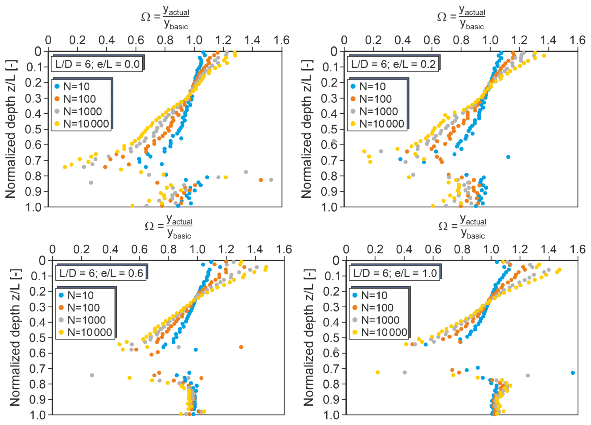
Figure 11Correction factors Ω for monopiles with 6 and different load eccentricities (very dense sand).

Figure 12Correction factors Ω for monopiles with 7 and different load eccentricities (very dense sand).
Figures 11 to 13 show the depth-dependent correction factors determined for relative monopile embedment lengths of 6, 7 and 8. Evidently, also the embedment length of the monopile at least slightly affects the correction factors. In all cases, correction factors greater than unity apply only at shallow depths down to approximately 0.2. However, the inclination of the correction factor curve above the rotation point increases with increasing and the almost constant values below the rotation point decrease slightly with increasing .
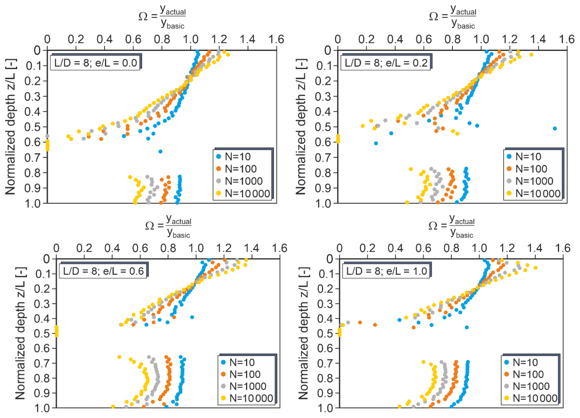
Figure 13Correction factors Ω for monopiles with 8 and different load eccentricities (very dense sand).
The following approach for calculation of the correction factor was found by systematic evaluation of the results of the parametric study conducted here.
Above the rotation point,
Below the rotation point, , where z is depth below sea bottom, L is embedment length of the pile ( 5–8), N is cycle numbers ( and e is load eccentricity (.
With the purpose of determining a suitable cyclic p–y curve under true loading conditions, this correction factor Ω has to be applied to the y multiplier of the basic overlay model. Hence, the following equation for the determination of cyclic y multipliers eventually results in
Users can apply these values on the displacements of a static p–y curve which was chosen by themselves to determine the cycle p–y curves at a desired cycle number.
It must be stated that Eq. (12) for the Ω value has only been calibrated for a pile diameter of D= 5 m and very dense sand as of yet. Supposedly, the relative density of sand does not have a great effect on the Ω values, but this has to be checked. A confirmation or extension of the Ω approach for piles of other diameters than 5 m will be done in a next step of the work.
The derived cyclic overlay model is an easy-to-use approach to predict the translocation of p–y curves due to lateral cyclic load for any static p–y approach. In the following, the overlay model is applied to the static p–y approach stated by API (2014) (see Sect. 2, Eqs. 1 and 2). The resulting deflections, bending moments and p–y curves can be compared to the results of the cyclic API approach, which is usually assumed to represent approximately 100 load cycles.
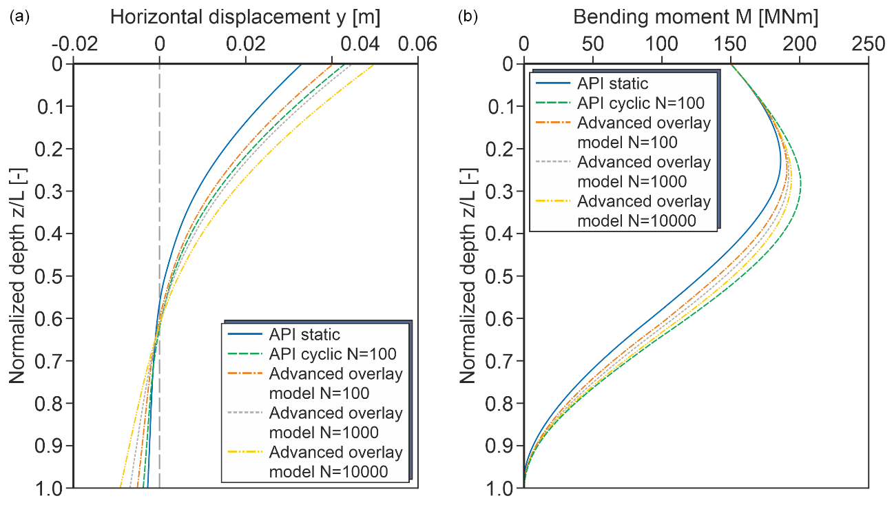
A monopile with a diameter of D = 5 m and an embedded length of L= 25 m ( 5) in very dense sand ( 40∘, 10.31 kN m−3; cf. Table 1) is considered. A constant wall thickness of t= 7 cm and a load eccentricity 0.6 are assumed.
Figure 14 shows deflection lines and bending moments for a horizontal load of H= 10 MN, calculated with the static API approach, the cyclic API approach and the cyclic overlay model for load cycle number of N= 100, 1000 and 10 000. The cyclic API approach predicts an increase of the pile head deflection (Fig. 14 left) with respect to the static approach of 30.5 %, which is in rather good agreement with the result of the cyclic overlay model for N= 100 (22.1 %). However, the overlay model also predicts pile head deflections for other load cycle numbers. For N= 1000 and 10 000, the head displacement increases by 35.6 % and 51.1 %, respectively.
Figure 14 right shows that the cyclic API approach overestimates the maximum bending moment of the monopile. Compared to the cyclic overlay model with N= 100, a 5.6 % greater maximum bending moment is gained. Also the bending moments of the cyclic overlay model with N= 1000 and 10 000 are considerably smaller than for the cyclic API approach.
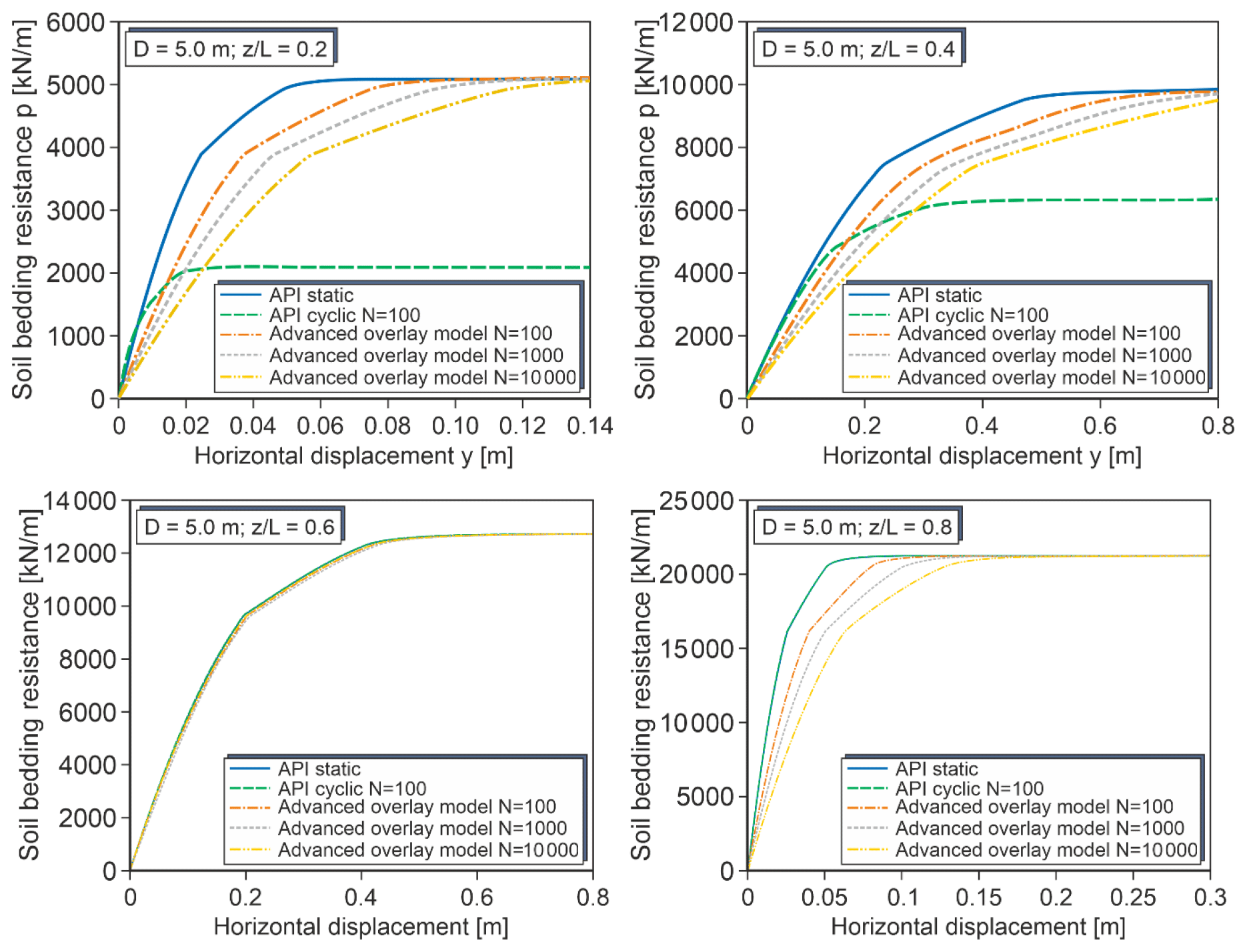
Figure 15 shows the reason for that. Here, the p–y curves at four distinct depths along the monopile are depicted. The cyclic API approach results in a severe degradation of bedding resistance and stiffness in shallow depth. In contrast, in greater depth (in this example below 0.525) no modification of the p–y curves is to be considered. For a stiff or almost rigid pile, this is of course unrealistic. It should be noted that the cyclic API approach was calibrated on lateral load tests on small and flexible piles. According to the cyclic overlay model, the p–y curves are subject to softening along the whole pile length. Therefore, at shallow depths much stiffer p–y curves apply, which results in considerably smaller maximum bending moments.
By comparison of numerical simulations of monopile behaviour once under monotonic and once under cyclic loading with a defined number of load cycles (utilizing the SDM), a cyclic p–y overlay model for monopiles in sand soils could be developed. Applying the derived equations for y multipliers, arbitrary p–y curves for monopile behaviour under monotonic loading can be adapted to a given number of load cycles. The y multipliers are formulated as a product of a term valid for constant horizontal deflection and a correction term accounting for the actual deflection line and loading conditions.
It was found that the first term could be formulated dependent only on the load cycle number and the angle of internal friction of the sand. In contrast, the second term was found to depend on load cycle number, monopile geometry (length-to-diameter ratio), load eccentricity and relative depth.
The new cyclic overlay model gives plausible results and can be applied to any monotonic p–y approach for monopiles in sand. However, an experimental validation of the model is still missing. It is planned to do this with cyclic large-scale pile load tests in an ongoing research project.
Abaqus input files can be made available upon request.
The result file can be made available upon request.
JS: conceptualization, methodology, investigation, and writing. MA: conceptualization, supervision, writing, and reviewing
The contact author has declared that neither of the authors has any competing interests.
Publisher’s note: Copernicus Publications remains neutral with regard to jurisdictional claims in published maps and institutional affiliations.
This study was carried out in the scope of the research project “Ho-Pile: Zyklische Erweiterung und experimentelle Validierung eines p–y-Ansatzes für Sand zur sicheren Monopilebemessung” funded by Bundesministerium für Wirtschaft und Energie (Germany, project no. 0324331A). The authors sincerely acknowledge BMWi support.
This research has been supported by the Projektträger Jülich (grant no. 324331A).
The publication of this article was funded by the open-access fund of Leibniz Universität Hannover.
This paper was edited by Lars Pilgaard Mikkelsen and reviewed by two anonymous referees.
Abaqus: Standard User's Manual, Version 6.14. Dassault Systèmes Simulia Corp, http://130.149.89.49:2080/v6.14/ (last access: 20 September 2021), 2016.
Achmus, M., Kuo, Y.-S., and Abdel-Rahman, K.: Behavior of monopile foundations under cyclic lateral load, Comput. Geotech., 36, 725–735, 2009.
Albiker, J.: Untersuchungen zum Tragverhalten zyklisch lateral belasteter Pfähle in nichtbindigen Böden, PhD Thesis, Leibniz Universität Hannover, Institute for Geotechnical Engineering, Vol. 77, 2016.
Albiker, J. and Achmus, M.: Development and validation of a numerically derived scheme to assess the cyclic performance of monopile foundations for offshore wind energy converters, 9th European Conference on Numerical Methods in Geotechnical Engineering (NUMGE), Porto/Portugal, 25–27 June 2018, ISBN 978-113854446-8, 2018.
API: Recommended Practice 2GEO-Geotechnical and Foundation Design Considerations, American Petroleum Institute, Version October 2014, 2014.
Burd, H. J., Taborda, D. M. G., Zdravković, L., Abadie, C. N., Byrne, B. W., Houlsby, G. T., Gavin, K. G., Igoe, D. J. P., Jardine, R. J., Martin, C. M., McAdam, R., Pedro, A. M. G., and Potts, D. M.: PISA design model for monopiles for offshore wind turbines: application to a marine sand, Geotechnique, 70, 1048–1066, https://doi.org/10.1680/jgeot.18.P.277, 2020.
Byrne, B. W., McAdam, R., Burd, H. J., Houlsby, G. T., Martin, C. M., Zdravković, L., Taborda, D. M G., Potts, D. M., Jardine, R. J., Sideri, M., Schroeder, F. C., Gavin, K., Doherty, P., Igoe, D., Muirwood, A., Kallehave, D., and Skov Gretlund, J.: New design methods for large diameter piles under lateral loading for offshore wind applications. Proceedings of the Third International Symposium of Frontiers in Offshore Geotechnics (ISFOG 2015), Oslo, Norway, ISBN 978-113802850-0, 2015.
Byrne, B. W., McAdam, R. A., Burd, H. J., Houlsby, C. T., Martin, C. M., and Plummer, M. A. L.: PISA: New design methods for offshore wind turbine monopiles, Proceedings of the 8th International Conference Offshore Site Investigations and Geotechnics (OSIG), London/UK, https://doi.org/10.3723/OSIG17.142, 2017.
Cox, W. R., Reese, L. C., and Grubbs, B. R.: Field Testing of Laterally Loaded Piles in Sand, Proceedings of the Offshore Technology Conference (OTC), Paper No. OTC 2079, ISBN 978-155563634-0, https://doi.org/10.4043/2079-ms, 1974.
Dührkop, J.: Zum Einfluss von Aufweitungen und zyklischen Lasten auf das Verformungsverhalten lateral beanspruchter Pfähle in Sand, PhD Thesis, Institut für Geotechnik und Baubetrieb, Technische Universität Hamburg-Harburg, Vol. 20, ISBN 978-3-936310-21-4, 2009 (in German).
Hettler, A.: Verschiebungen starrer und elastischer Gründungskörper in Sand bei monotoner und zyklischer Belastung, PhD Thesis, Department of Civil Engineering, Geo- and Environmental Sciences, Institute of Soil Mechanics and Rock Mechanics, University of Karlsruhe, Germany, 1981 (in German).
Huurman, M.: Development of traffic induced permanent strains in concrete block pavements, Heron, 41, 29–52, 1996.
Kallehave, D., LeBlanc Thilsted, C., and Liingaard, M. A.: Modification of the API p-y formulation of initial stiffness of sand. Proceedings of the 7th International Conference Offshore Site Investigation and Geotechnics, London/ UK, 465–472, https://onepetro.org/SUTOSIG/proceedings-abstract/OSIG12/All-OSIG12/SUT-OSIG-12-50/3358 (last access: 20 September 2021), 2012.
Kuo, Y.-S.: On the behavior of large-diameter piles under cyclic lateral load, PhD thesis, Leibniz Universität Hannover, Hannover, Institute for Geotechnical Engineering, Vol. 65, 2008.
Kuo, Y.-S., Achmus, M., and Abdel-Rahman, K.: Minimum embedded length of cyclic horizontally loaded monopiles, J. Geotech. Geoenviron., 138, 357–363, 2012.
LeBlanc, C., Houlsby, G. T., and Byrne, B. W.: Response of stiff piles in sand to long-term cyclic lateral loading, Géotechnique, 60, 79–90, 2010.
Lin, S. S. and Liao, J. C.: Permanent strains of piles in sand due to cyclic lateral loads, J. Geotech. Eng.-ASCE, 125, 798–802, 1999.
Little, R. L. and Briaud, J. L.: Full scale cyclic lateral load tests on six single piles in sand. Miscellaneous paper GL-88-27, Texas: Geotechnical Division, Texas A&M University, https://www.semanticscholar.org/paper/Full-Scale-Cyclic-Lateral-Load-Tests-on-Six-Single-Little-Briaud/73330ddfbbd92d119166f3df241791bfd85ffa65#citing-papers (last acess: 20 September 2021), 1988.
Long, J. H. and Vanneste, G.: Effect of cyclic lateral loads on piles in sand, J. Geotech. Eng.-ASCE, 120, 33–42, 1994.
Peralta, P. and Achmus, M.: An Experimental Investigation of Piles in Sand Subjected to Lateral Cyclic Loads, 7th International Conference on Physical Modeling in Geotechnics (ICPMG 2010), Zurich, Switzerland, 28 June–1 July 2010, ISBN 978-041559290-1, 2010.
Sørensen, S. P. H.: Soil-structure interaction for non-slender large-diameter offshore monopiles, PhD Thesis, Aalborg University Denmark, Department of Civil Engineering, e-ISBN 9788792982360, 2012.
Thieken, K., Achmus, M., Lemke, K., and Terceros, M.: Evaluation of p-y approaches for large diameter monopiles in sand, Int. J. Offshore Polar, 25 134–144, 2015a.
Thieken, K., Achmus, M., and Lemke, K.: A new static p-y approach for piles with arbitrary dimensions in sand, Geotechnik, 38, 267–288, 2015b.