OC6 project Phase III: validation of the aerodynamic loading on a wind turbine rotor undergoing large motion caused by a floating support structure

This paper provides a summary of the work done within Phase III of the Offshore Code Comparison Collaboration, Continued, with Correlation and unCertainty (OC6) project, under the International Energy Agency Wind Technology Collaboration Programme Task 30. This phase focused on validating the aerodynamic loading on a wind turbine rotor undergoing large motion caused by a floating support structure. Numerical models of the Technical University of Denmark 10 MW reference wind turbine were validated using measurement data from a 1:75 scale test performed during the UNsteady Aerodynamics for FLOating Wind (UNAFLOW) project and a follow-on experimental campaign, both performed at the Politecnico di Milano wind tunnel. Validation of the models was performed by comparing the loads for steady (fixed platform) and unsteady (harmonic motion of the platform) wind conditions. For the unsteady wind conditions, the platform was forced to oscillate in the surge and pitch directions under several frequencies and amplitudes. These oscillations result in a wind variation that impacts the rotor loads (e.g., thrust and torque). For the conditions studied in these tests, the system aerodynamic response was almost steady. Only a small hysteresis in airfoil performance undergoing angle of attack variations in attached flow was observed. During the experiments, the rotor speed and blade pitch angle were held constant. However, in real wind turbine operating conditions, the surge and pitch variations would result in rotor speed variations and/or blade pitch actuations, depending on the wind turbine controller region that the system is operating. Additional simulations with these control parameters were conducted to verify the fidelity of different models. Participant results showed, in general, a good agreement with the experimental measurements and the need to account for dynamic inflow when there are changes in the flow conditions due to the rotor speed variations or blade pitch actuations in response to surge and pitch motion. Numerical models not accounting for dynamic inflow effects predicted rotor loads that were 9 % lower in amplitude during rotor speed variations and 18 % higher in amplitude during blade pitch actuations.

1 Introduction

The objective of Phase III of the Offshore Code Comparison Collaboration, Continued, with Correlation and unCertainty (OC6) project is to evaluate the accuracy of aerodynamic load predictions by offshore wind modeling tools for a floating offshore wind turbine (FOWT). FOWT platforms can experience significant translational and rotational motions, affecting the system dynamics and loads (Veers et al., 2022).

The OC6 project is part of an ongoing effort under the International Energy Agency Wind Technology Collaboration Programme (IEA Wind) Task 30 to verify and validate offshore wind turbine modeling tools (IEA Wind, 2022). To validate the aerodynamic loading on the wind turbine under large motions, participants in OC6 Phase III modeled a 1:75 scaled version of the Technical University of Denmark (DTU) 10 MW reference wind turbine (RWT) (Bak et al., 2013) examined in the Unsteady Aerodynamics for FLOating Wind (UNAFLOW) project (Fontanella et al., 2021a, b) and a follow-on experimental campaign. For such configuration, the group ran a series of simulations, including steady and unsteady wind conditions due to the platform motion, and compared the resulting rotor loads and wake behavior from the experiments and the different modeling tools. The rotor loads were also compared between different modeling approaches to assess the potential advantages and disadvantages of models of different fidelities. This paper summarizes the work done within the OC6 Phase III project.

Table 1 Distributed blade properties.

The organization of the remainder of the paper is as follows: Sect. 2 provides a definition of the scaled model and testing performed. Section 3 provides a description of the active participants involved in OC6 Phase III and their modeling approaches. Section 4 then summarizes the load cases that were performed for the verification and validation. Finally, Sects. 5 and 6 provide some example results from the project and the conclusions drawn.

2 Model definition

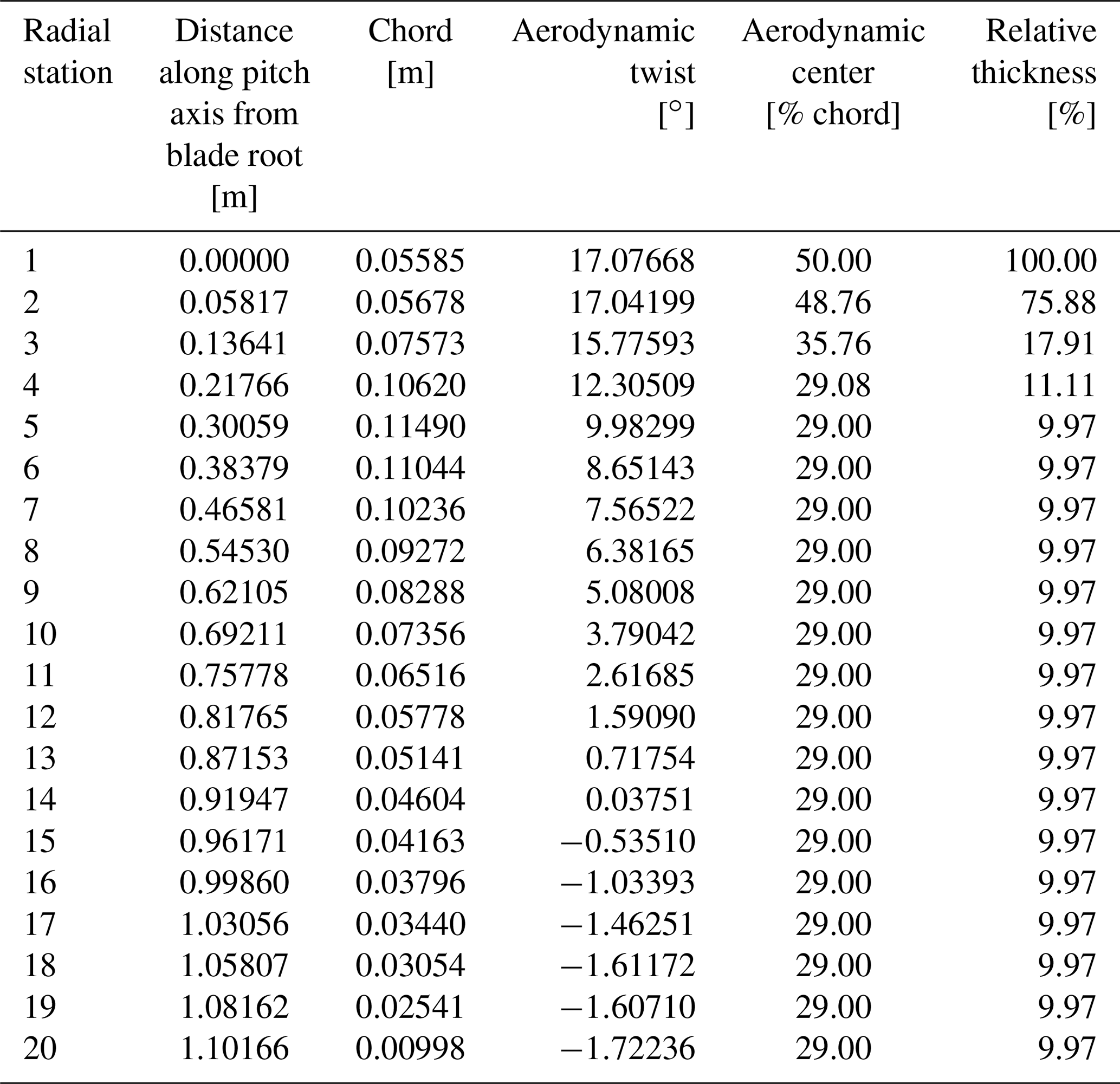
To validate the accuracy of the rotor loads for an FOWT, measurement data from two wind tunnel experimental campaigns were used. Both campaigns were conducted in the Politecnico di Milano wind tunnel (13.84 m wide by 3.84 m high by 35 m long) and used a 1:75 scaled version of the DTU 10 MW RWT. The blades were straight, without a cone angle, and rigid. The blade properties can be found in Table 1. The aerodynamic center of the different radial stations is coincident with the blade pitch axis. Its position along the chord, as measured from the leading edge, is given in Table 1.

Two-dimensional sectional-model experiments were conducted in the DTU red wind tunnel to characterize the airfoil polars with smooth- and rough-surface conditions (Fontanella et al., 2021b). The airfoil polars, with the lift and drag coefficients for the different angles of attack at the 20 radial stations shown in Table 1 for rough-surface conditions, were provided to the participants. Each airfoil polar contains seven sets of lift and drag coefficients for Reynolds numbers ranging between 5E4 and 2E5 (Robertson et al., 2023).

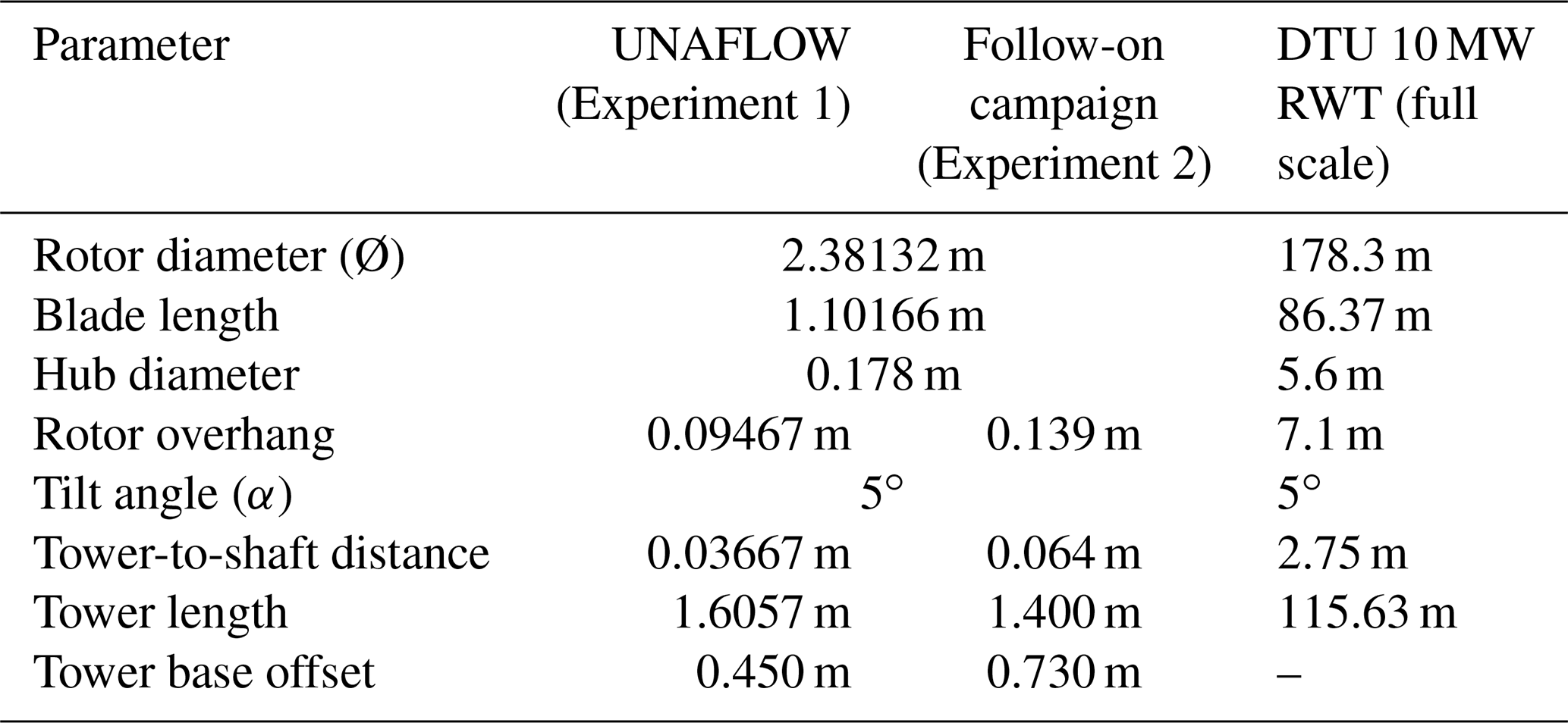
The rest of the model geometry (e.g., tower, rotor overhang) was dependent on the testing campaign being studied. The first data set was developed during the UNAFLOW project (Fontanella et al., 2021a). The testing was similar to that performed during the LIFES50+ project (Bayati et al., 2017). However, for the UNAFLOW test the tower was considered rigid and included a negative tilt angle of 5^∘ to offset the wind turbine tilt angle, resulting in a rotor perpendicular to the wind tunnel floor. The second data set is from a follow-on testing campaign performed during 2021 in the same wind tunnel. It used the same rotor but a different nacelle and tower length (also rigid) than the one used in the UNAFLOW project.

Figure 1 shows the scaled DTU 10 MW RWT during the two testing campaigns. For simplicity, the UNAFLOW campaign is described as Experiment 1, and the follow-on campaign is described as Experiment 2. An air density of 1.177 kg m⁻³ is considered for both campaigns.

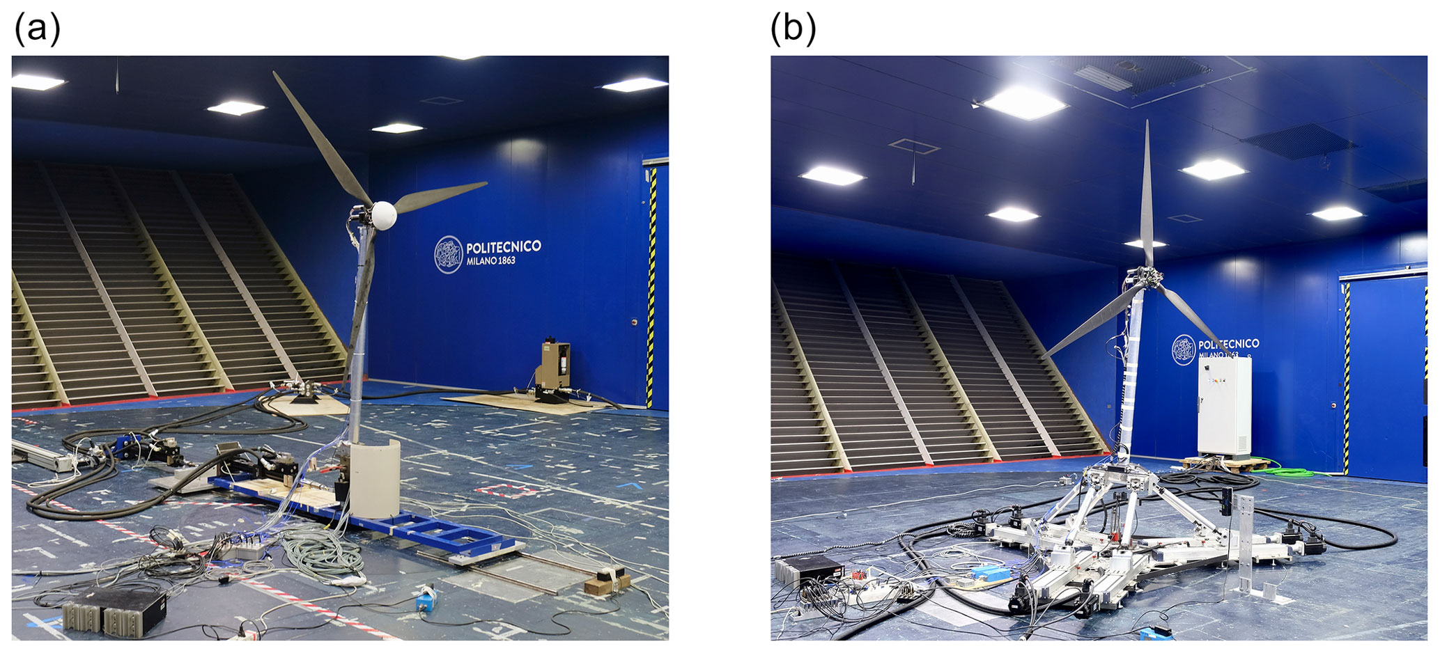
Figure 1 The 1:75 scaled DTU 10 MW reference wind turbine in the Politecnico di Milano wind tunnel. (a) Testing during the UNAFLOW campaign (Experiment 1). (b) Testing during the follow-on campaign (Experiment 2).

Figure 2 shows a schematic representation of the wind turbine tested in both campaigns and the two coordinate systems used in this project. Table 2 provides the geometrical properties for these two campaigns.

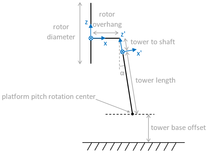
Figure 2 Schematic representation of the wind turbine system and the coordinate systems (hub fix and tower top).

Table 2 System geometry.

Experiment 1 includes steady and unsteady wind conditions. The unsteady wind conditions were induced by means of forced harmonic oscillations in the surge direction (i.e., fore–aft translation). The forced motion was achieved through two hydraulic actuators at the tower base. This campaign includes load measurements with a 6 degree of freedom (DOF) load cell at the tower-top location, a 6 DOF load cell at the tower base, hot-wire probes to measure the wind speed along and across the wake, and particle image velocimetry (PIV) to study the blade-tip vortex behavior.

Experiment 2 used a 6 DOF robot at the base instead of the two hydraulic actuators used for the fore–aft translation in Experiment 1. During this testing, some of the conditions studied during Experiment 1 were tested again. In addition, for the unsteady wind cases, equivalent tests resulting in the same rotor apparent wind were tested but using platform pitch motion instead of surge motion. Equivalent measurements for tower-top loads were recorded during this test campaign, but information about the wind turbine wake was not recorded (i.e., hot-wire and PIV measurements are not available).

During Experiment 1, the rotor was kept rotating at a constant speed. However, Experiment 2 used a different rotor speed controller, resulting in some rotor speed oscillations. These rotor speed variations can impact the amplitude and phase of the rotor loads, which could have important implications for the torque due to the rotor inertia. Politecnico di Milano tried to remove these rotor speed variations by means of an analytical postprocessing.

The hub height in both experiments is also slightly different. The relatively small distance (close to 0.5 m or 0.2 rotor diameter) between the blade tip and the wind tunnel ceiling might affect the wake expansion in the vertical direction and thus the induction in the rotor area.

During the testing campaigns, the wind turbulence intensity in the region covered by the rotor was close to 2 % (Bayati et al., 2018). Moreover, the wind speed was fairly constant over the rotor-swept area (Bayati et al., 2018). For the numerical models, it was decided to use a spatially uniform steady inflow.

Finally, Politecnico di Milano performed a postprocessing of the load measurements to remove the inertial loads (Mancini, 2020). The loads studied in this paper are purely aerodynamic. Participants modeled a rigid tower and a rigid rotor and extracted the rotor aerodynamic loads.

3 Participants and modeling approach

A total of 29 academic and industrial partners from 10 different countries participated in OC6 Phase III. Those actively involved were Bureau Veritas (BVMO, France), the Centro Nacional de Energías Renovables (CENER, Spain), the China General Certification Center (CGC, China), the China State Shipbuilding Corporation (CSSC, China), Det Norsk Veritas (DNV, United Kingdom), the Technical University of Denmark (DTU, Denmark), the Dalian University of Technology (DUT, China), Électricité de France (EDF, France), eureka! (EURE, Spain), the Institute for Energy Technology (IFE, Norway), IFP Energies nouvelles (IFPEN, France), the Maritime Research Institute Netherlands (MAR, the Netherlands), the National Renewable Energy Laboratory (NREL, USA), Newcastle University (NU, United Kingdom), the Office National d'Etudes et de Recherches Aérospatiales (ON, France), Politecnico di Milano – the POLI-Wind Laboratory (POLI-W, Italy), Politecnico di Milano (POLIMI, Italy), PRINCIPIA (PRI, France), Shanghai Jiao Tong University (SJTU, China), Tecnalia (TECN, Spain), the Netherlands Organization for Applied Scientific Research (TNO, the Netherlands), Technische Universität Berlin (TUB, Germany), Hamburg University of Technology (TUHH, Germany), Università degli Studi di Firenze (UNIFI, Italy), Universitat Politècnica de Catalunya (UPC, Spain), the University of Stuttgart (USTUTT, Germany), the University of Strathclyde (UoS, United Kingdom), Vulcain Engineering (VULC, France), and WyndTek (WTEK, the Netherlands).

The participants used modeling approaches of different fidelities to study the system: blade element momentum (BEM) theory, dynamic BEM (DBEM) that accounts for a dynamic inflow effect, generalized dynamic wake (GDW), free-vortex wake (FVW), and blade-resolved or actuator-line-based computational fluid dynamics (CFD).

The BEM, DBEM, GDW, some FVW, and the actuator-line-based CFD approaches are based on the lifting-line theory. In these approaches, the airfoil polar data are used as an input for the model. The airfoil polar provides information about the lift and drag coefficients as a function of the angle of attack. Participants can use the airfoil polar information as a look-up table (static polar approach) or to account for unsteady airfoil aerodynamics. The unsteady airfoil aerodynamics accounts for the flow hysteresis in the lift and drag coefficients under unsteady wind and wind turbine operating conditions (e.g., blade pitch actuations). The flow hysteresis can occur during attached flow (e.g., linear region in the airfoil polar) or flow separation, including dynamic stall (e.g., nonlinear region in the airfoil polar). These unsteady effects are computed by the modeling tools and depend on the underlying theory considered. The lifting surface and three-dimensional panel FVW as well as the blade-resolved CFD do not use the airfoil polar data as input. Instead, they use a surface mesh based on the blade geometry. One computer-aided design (CAD) file of the blade was provided to the participants. In this case, it may be challenging to reproduce the airfoil polars' behavior due to the relatively small Reynolds numbers during the experiment (mainly below 1E5). Small Reynolds numbers may increase the boundary-layer thickness, resulting in larger drag and smaller lift coefficients.

Sectional aerodynamic loads are computed on the basis of the local inflow velocity. The local inflow velocity is the sum of the relative velocity (e.g., due to the incoming wind, the rotor rotation, and the platform motion) and the induced velocity (i.e., the velocity change due to the interaction with the rotor). The steady BEM theory assumes that the wake reacts instantaneously. In this equilibrium wake assumption, the induced velocities (based on the axial and tangential induction factors) are quasi-steady. However, in reality, it takes time (delay) for the wake to respond to a change in the flow conditions. This change in the flow conditions can be due to changes in the incoming wind or the turbine response (e.g., rotor speed variations, blade pitch variations, and platform motions). The BEM theory with a dynamic inflow model (also referred to as dynamic wake) tries to capture the unsteady aerodynamic response from this delayed wake response by means of a correction consisting of low-pass filters over the quasi-steady induced velocities. In GDW, dynamic inflow is explicitly calculated by representing the induced velocity in terms of series expansion of radial and azimuthal basis functions within a governing equation that takes into account an apparent mass. Dynamic inflow is intrinsically captured by FVW because induction is calculated directly from the time-dependent trailing and shed vorticity and by CFD because of the explicit solving of the momentum and continuity equations.

A list of the participants is provided in Table 3, which also shows the modeling approaches adopted and the codes used. Some participants decided to use more than one modeling approach, and some used different codes. A total of 54 numerical models were involved in this validation.

Table 3 Summary of participants, codes, and modeling approach used.

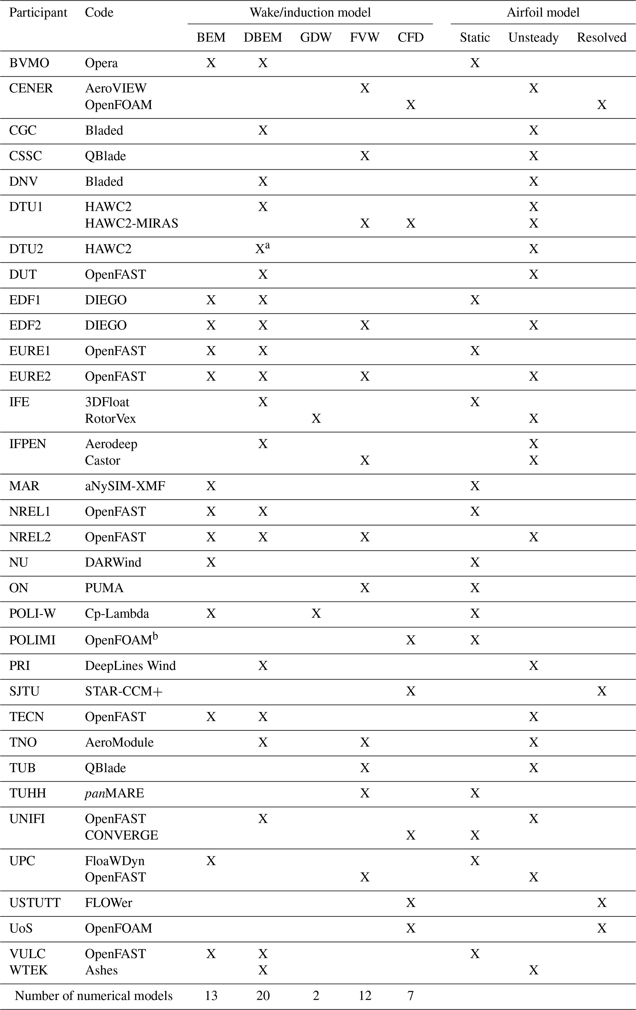
^a Near-wake model. ^b OpenFOAM modified version.

EDF, EURE, and NREL used two different modeling approaches based on the lifting-line theory within the same code. The models denoted with “1” use a static polar approach, while the models denoted with “2” account for unsteady airfoil aerodynamics.

Other participants using a lifting-line approach with static polars were BVMO, IFE (DBEM), MAR, NU, ON, POLI-W, POLIMI, TUHH, UNIFI (FVW), UPC (BEM), and VULC. Other participants using a lifting-line approach with unsteady airfoil aerodynamics were CENER (FVW), CGC, CSSC, DNV, DTU1, DTU2, DUT, IFE (GDW), IFPEN, PRI, TECN, TNO, TUB, UNIFI (DBEM), UPC (FVW), and WTEK.

All FVW models used by participants are based on the lifting-line theory. For the CFD models, three participants used an actuator-line-based approach (DTU1, POLIMI, and UNIFI), and four participants used a blade-resolved approach (CENER, SJTU, USTUTT, and UoS).

4 Load cases

A stepwise validation procedure was performed in the OC6 Phase III project, taking advantage of the two experimental campaigns carried out in the Politecnico di Milano wind tunnel.

Table 4 provides a summary of the simulations that are presented in Sect. 5, including one steady wind condition (Load Case 1.1) and unsteady wind conditions under platform surge (Load Cases 2.X) and platform pitch motion (Load Cases 3.X). For the pitch motion, the equivalent longitudinal amplitude can be approximated by multiplying the sine of the platform pitch angle by the distance from the hub to the tower base. Load Cases 3.5 and 3.7 result in the same rotor apparent wind (horizontal component) as Load Cases 2.5 and 2.7, respectively. The rotor apparent wind in Load Case 3.1 is slightly lower than in Load Case 2.1 due to a limitation in the 6 DOF robot motion range.

Table 4 Offshore Code Comparison Collaboration, Continued, with Correlation and unCertainty (OC6) Phase III load case simulations (summary).

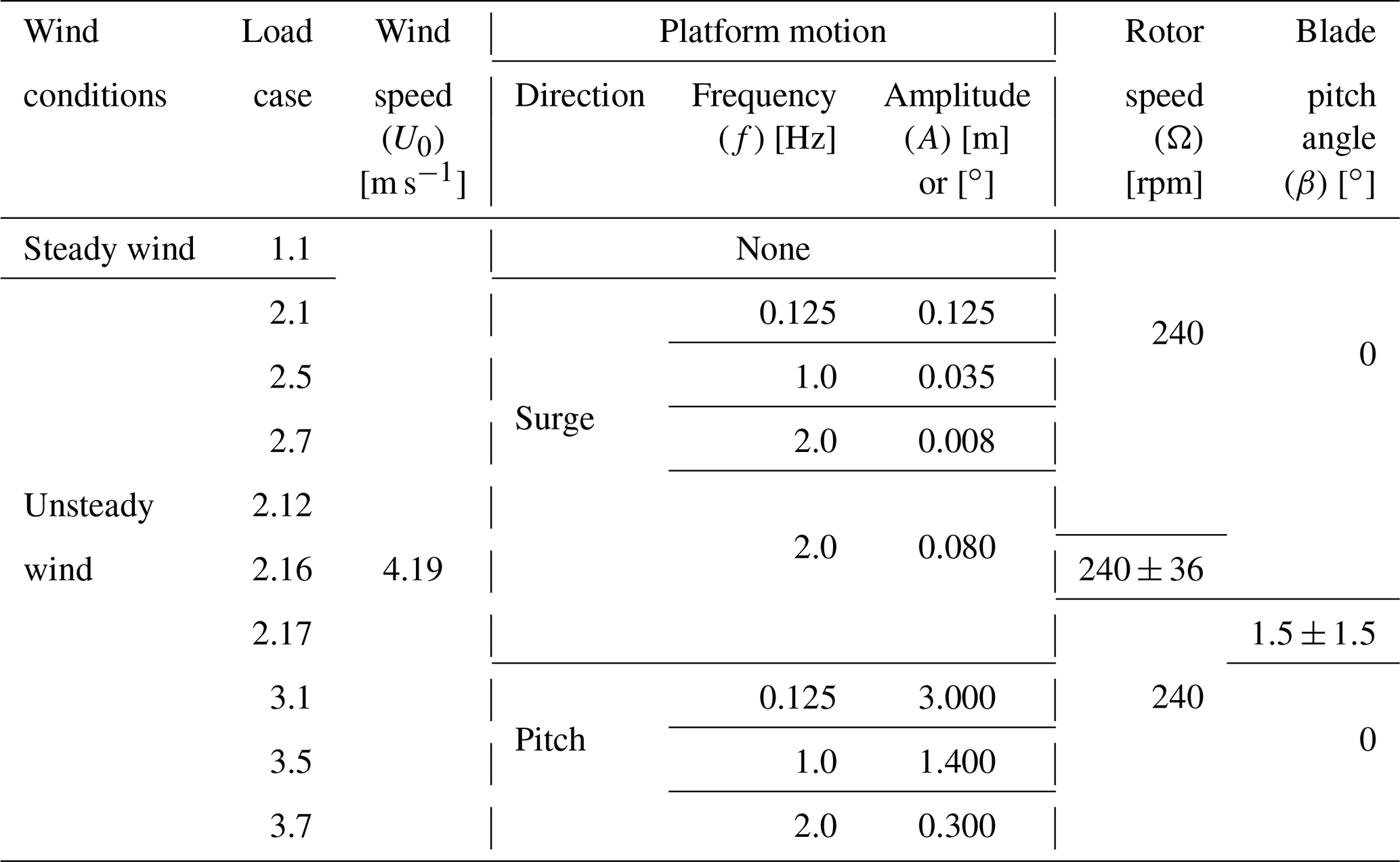
Three additional load cases (2.12, 2.16, and 2.17) were included to examine conditions that might create more impactful unsteady aerodynamic responses due to changes in the flow conditions. There are no experimental data available for these conditions; thus, they are used as verification cases only. Load Case 2.12 includes a platform surge oscillation at the same frequency as Load Case 2.7 but with an amplitude that is 1 order of magnitude higher. Finally, Load Cases 2.16 and 2.17 are based on Load Case 2.12 but include some rotor speed and blade pitch variations.

Some numbers are skipped in the load case numbering sequence because there were more load cases that did not provide additional insight and are therefore left out of the results of Sect. 5.

The studied wind speed of 4.19 m s⁻¹ and rotor speed of 240 rpm in these load cases is representative of the near-rated condition for the DTU 10 MW RWT at a model scale (tip-speed ratio of 7.1). This wind speed was already corrected to account for the wind tunnel blockage (Robertson et al., 2023). The presence of the scaled wind turbine in the test section reduces the flow area compared to an unrestricted freestream. This flow area reduction results in an increased wind velocity in the rotor disk area. The blockage ratio between the rotor disk area and the wind tunnel cross area was close to 8 % during the experiments. This corrected value of 4.19 m s⁻¹ was used by participants using BEM, DBEM, GDW, and FVW approaches. Most participants using the CFD approach (POLIMI, UNIFI, USTUTT, and UoS) included the wind tunnel walls, ceiling, and floor in their numerical models, reproducing the confined system conditions. These boundary conditions were introduced in the CFD models by means of slip walls. A wind speed of 4 m s⁻¹ was used by these participants.

In the study of unsteady aerodynamics, it is common to use reduced frequencies (Ferreira et al., 2022; Mancini et al., 2020). The reduced frequency is a dimensionless number with higher values, indicating a greater degree of unsteadiness. The rotor's reduced frequency (k) is related to the motion frequency (f), the rotor diameter (Ø), and the freestream wind (U₀) as stated in Eq. (1). The platform motion frequencies shown in Table 4 result in the rotor's reduced frequencies of 0.071, 0.568, and 1.137.

$$\begin{array}{}\text{(1)}& k=f\cdot {\displaystyle \frac{\mathrm{Ø}}{U_{\mathrm{0}}}}\end{array}$$

The platform motion amplitudes shown in Table 4 correspond to oscillations ranging from 0.6 to 9.375 m at a full scale (i.e., from 0.003 to 0.05 rotor diameter). In terms of periods at a full scale, the tests cover the range from 12.5 to 20 s (Mancini et al., 2020). Most FOWT testing is done with Froude-scaled models. However, in the two testing campaigns considered in this study, the scaling was based on the reduced frequency to try to preserve the relationship between the wind and the platform velocity. In this case, the wind velocity was scaled by a factor of 3 and the physical dimensions by 75 (Mancini et al., 2020). These amplitudes and periods are considered representative of different FOWT support structures.

The loads measured at the tower top during the experiments were oriented according to the tilted tower (x^′–y^′–z^′ coordinate system in Fig. 2). These loads were first rotated according to the tilt angle and then translated to the hub location (x–y–z coordinate system in Fig. 2) to make the comparison between the numerical models and the experiments easier.

During the processing of the experimental data, a significant 1P response corresponding to the blade-passing frequency was observed. This frequency was due to a rotor asymmetry. The three blades were weighted, and one of the blades had a significant mass imbalance (∼10 %). Moreover, a 2P was also present in the response. This could imply an aerodynamic imbalance (e.g., one blade pitch error or blades with different aerodynamic performances). This aerodynamic imbalance would result in loads with a different mean value as well as the presence of a 1P in the response and the corresponding harmonics (e.g., 2P). To avoid the dynamic influence of this rotor asymmetry, the data from the experiments were low-pass filtered at 3 Hz. This cutoff frequency was a compromise to include the fastest platform motion in the experiments (2 Hz in Load Cases 2.7 and 3.7) and exclude the rotor asymmetry (1P frequency is 4 Hz for a rotational speed of 240 rpm). The low-pass filter also removes the tower shadow effect (e.g., the 3P excitation and the corresponding harmonics). Accordingly, participants did not include the tower's influence on the wind in their numerical models, or they filtered it out in the case it was included.

5 Results

In this section, a comprehensive overview of the studied load cases shown in Table 4 is presented and explained.

5.1 Steady wind: Load Case 1.1

5.1.1 Aerodynamic rotor loads

Load Case 1.1 focuses on ensuring that the aerodynamic models were implemented correctly by examining the aerodynamic rotor loads. The rotor is perpendicular to the tunnel floor (i.e., there is no effective tilt angle), spatially uniform wind is considered, and the tower's influence over the wind is not considered. Therefore, the resultant rotor loads are only F_x (thrust force) and M_x (torque).

Figure 3 shows the aerodynamic rotor thrust for Load Case 1.1. Figure 3 includes the results from the participants, grouped according to the modeling approach from lower to higher fidelity (BEM < DBEM ≈ GDW < FVW < CFD). The results from the two experimental campaigns are also included. There is a difference in the aerodynamic thrust between the two experiments (7 %). Experiment 1 shows less variation in the mean aerodynamic forces during the testing, indicating more reliable measurements. This difference in Experiment 2 could be due to the influence of the cable bundle used for the sensors and power that is located behind the wind turbine (see Fig. 1) or a small blade pitch angle offset.

Figure 3 Aerodynamic rotor thrust in steady wind conditions (Load Case 1.1).

Figure 4 Aerodynamic rotor torque in steady wind conditions (Load Case 1.1).

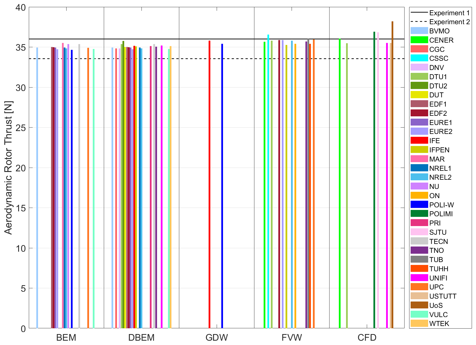
As Fig. 3 shows, most numerical models predict an aerodynamic thrust force that is within the values observed in the experiments. Only some FVW and CFD solutions are slightly above the values observed in Experiment 1. FVW solutions (based on the lifting-line theory) return higher thrust values than BEM and DBEM solutions despite using the same airfoil polar data. When looking at the local inflow velocity along the blade (not shown), it can be noticed that the FVW models have slightly higher values. Since the rotational speed is fixed and the incoming wind is the same, this indicates that the FVW models have slightly different induction factors. By looking at the axial and tangential induction (not shown), FVW models have lower axial and higher tangential induction factors with both contributions adding to a higher local inflow velocity. Moreover, the lower axial induction factor in the FVW results in a higher angle of attack. Both the higher local inflow velocity and the higher angle of attack result in higher loads.

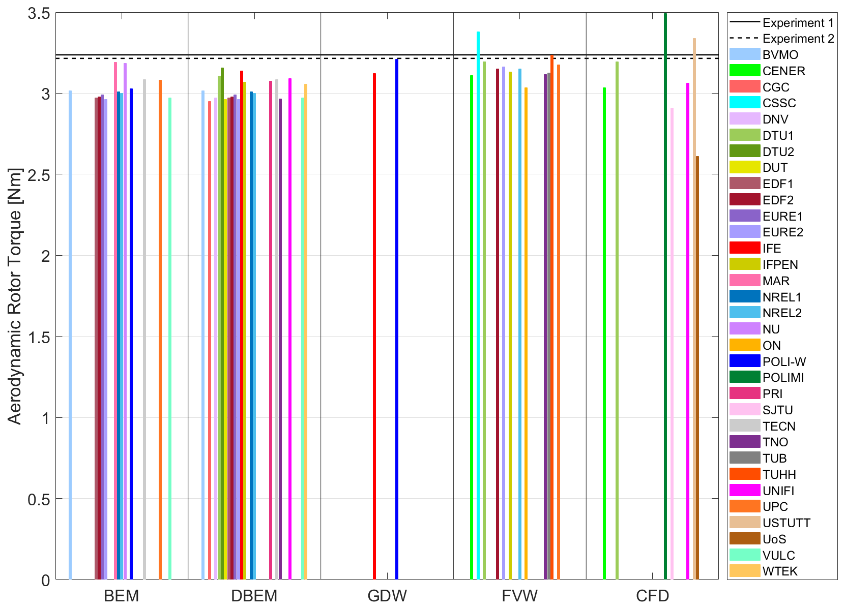
Figure 4 shows the corresponding aerodynamic rotor torque for Load Case 1.1. There is a good agreement between both experiments, while most numerical models underpredict the aerodynamic torque.

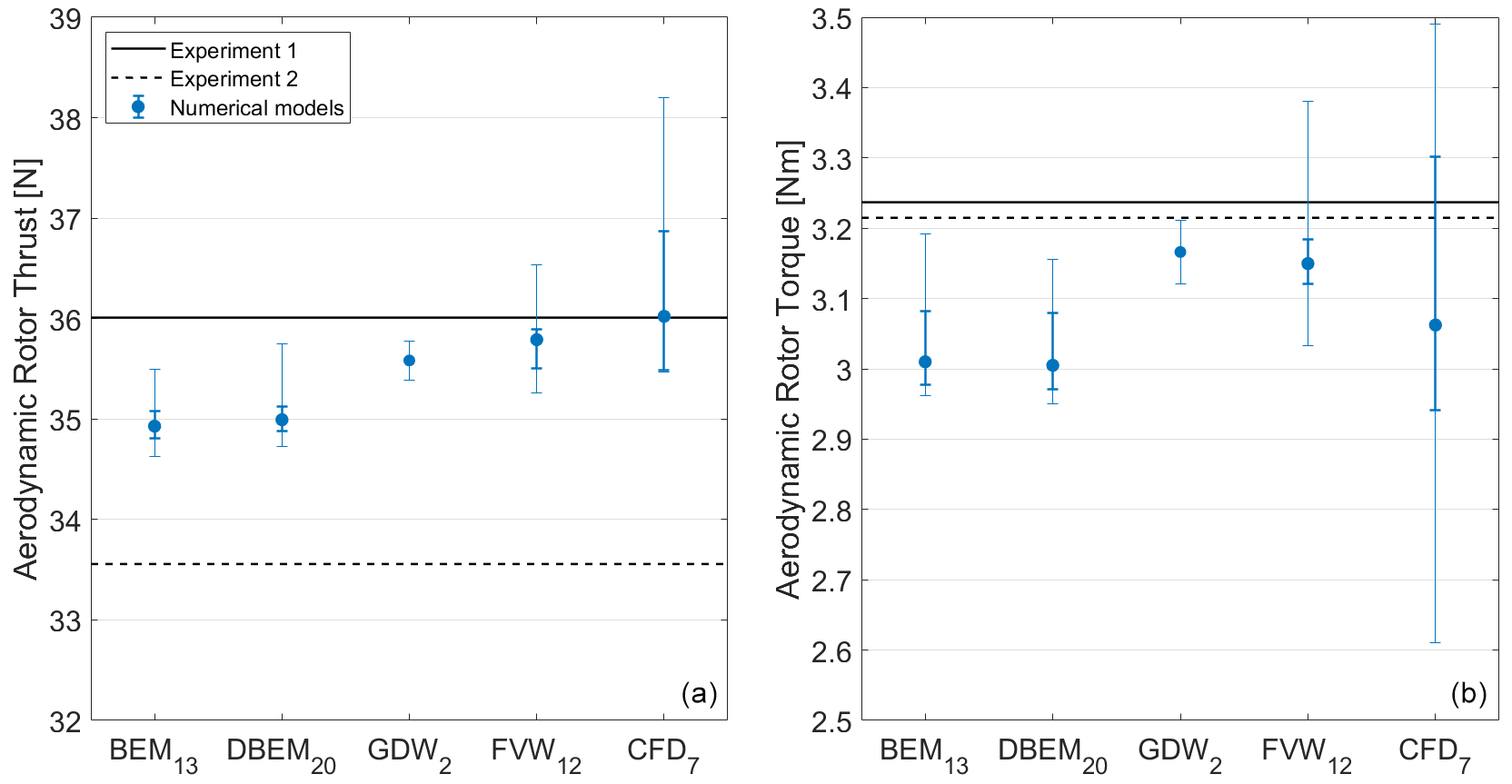
Figure 5 Aerodynamic rotor thrust (a) and torque (b) during the steady wind condition. Median and quartiles for the different simulation approaches.

For steady wind conditions, no differences between BEM and DBEM are expected because there are no variations in terms of wind, rotor speed, or blade pitch angle. This expected behavior is observed within the participants using the same code with BEM and DBEM (i.e., BVMO, EDF, EURE, NREL, TECN, and VULC). Moreover, no differences between static polars and unsteady airfoil aerodynamics are expected because the angle of attack at each blade radial station is constant, and the rotor is planar (Li et al., 2022).

Most BEM and DBEM models account for aerodynamic corrections commonly used in the design of wind turbines (e.g., blade-root and blade-tip losses). The lack of these corrections results in loads that are higher than expected.

Figure 5 presents a summary of the aerodynamic rotor thrust and torque based on the modeling approaches. The data from Figs. 3 and 4 have been sorted from lower to higher within each modeling approach and have been divided into four parts (quarters). The dots shown are indicative of the median (i.e., second quartile). The median and the quartiles provide information about both the center and the spread of the data. For example, the band around the median contains 50 % of the participant results for a given modeling approach. The upper and lower ranges contain the remaining 25 % of the participant results. This statistical information can be considered equivalent to that obtained from a boxplot. Using the median instead of the mean avoids the potential impact of outliers on the data. The subindex next to each modeling approach indicates the number of results available from the participants. For the GDW approach there are only data from two participants. In this case, the median is equivalent to the mean, and the range is determined by the maximum and minimum values.

5.1.2 Hot-wire measurements

For Experiment 1, hot-wire measurements were taken during the steady wind condition. A hot-wire anemometer probe traversed the along-wind direction (x direction in Fig. 6) and the crosswind direction (y direction in Fig. 6). Participants using FVW or CFD can get insights into the wind turbine wake behavior. For reference, Fig. 6 includes the wake behavior for NREL (FVW), as well as the hot-wire locations (black dots) and PIV plane (gray rectangle).

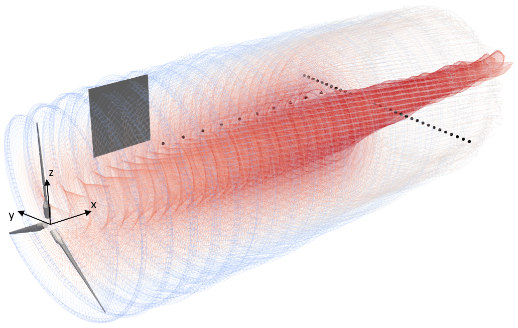
Figure 6 Wind turbine wake behavior in OpenFAST (free-vortex wake approach) during steady wind conditions.

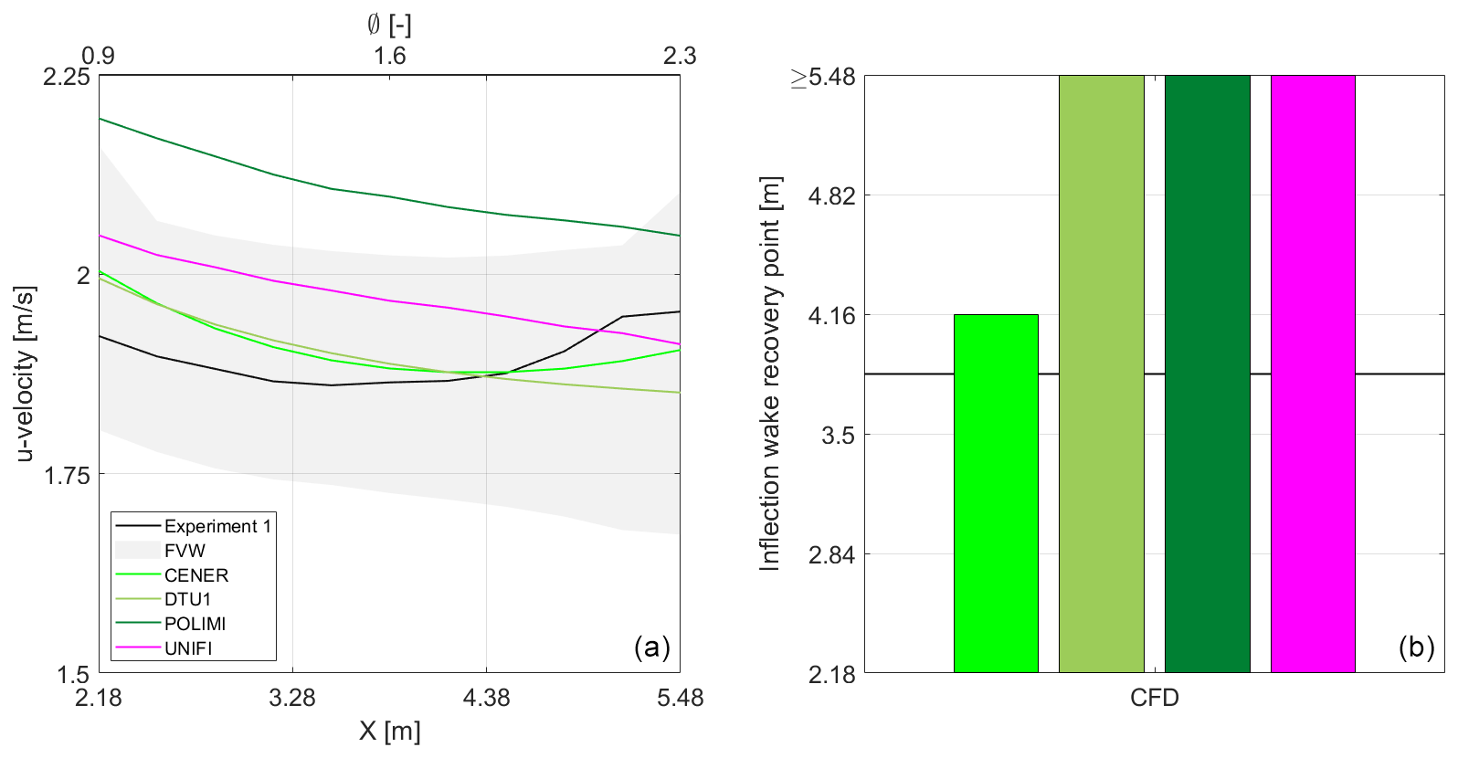
Figure 7 (a) Averaged hot-wire longitudinal velocity for one rotor revolution in the along-wind direction (y=0.9 m, z = hub height) during steady wind conditions. (b) Inflection wake recovery point location.

For the along-wind measurements, the hot-wire anemometer probe started with a 0.9 m offset in the y direction and moved between 2.18 and 5.48 m along the x direction from the hub location (i.e., 0.9 and 2.3 rotor diameters (Ø) downwind). Eleven points every 0.33 m along the x direction were measured. Figure 7a shows the corresponding longitudinal wind speed (u) measured by the hot-wire probe and the output from the FVW and CFD participants. The wind speed in the figure corresponds to the average value at the location of interest during one rotor revolution. The CFD solutions are denoted with a solid line, while the FVW solutions (12 outputs) are denoted by a gray area due to some limitations. For example, the wind speed obtained within the wake is a function of the wake length chosen by the FVW participants. Moreover, the lack of viscous diffusion in the FVW models makes the characterization of the wake recovery challenging in the absence of meandering from turbulence. Despite these limitations, we would expect a decent agreement between FVW approaches in the near wake because, in this region, the viscous diffusion should not be driving the wake response. However, a significant spread of results was observed for FVW participants. Figure 7b shows the inflection wake recovery point for the experiment and the CFD participants. This is the point where the wake velocity shows a minimum and from that point starts to recover. The outputs from individual FVW participants are not included for the reasons explained previously. It is also worth noting that the ambient turbulence observed in the wind tunnel should result in a shorter inflection wake recovery point. The ambient turbulence intensity during the testing was close to 2 % while participants considered a steady wind condition. The maximum wake velocity deficit observed in the experiment is around $u/U_{\mathrm{0}}=\mathrm{0.44}$. Most numerical models show a wind speed deficit like in the experiment. However, there are some differences regarding the inflection wake recovery point. For most CFD participants, the inflection wake recovery point occurs at a distance equal to or after 5.48 m (i.e., 2.3 diameters downwind).

Figure 8 (a) Averaged hot-wire longitudinal velocity for one rotor revolution in the crosswind direction (x=5.48 m, z = hub height) during steady wind conditions. (b) Average wake deficit within the rotor region.

As Fig. 7a shows, the last hot-wire measurement at the point 5.48 m downwind seems to be off. This results in a lower-than-expected wake slope at the end of the window studied. This unexpected behavior is not observed in other tests and measurements (see next section: analysis of the hot-wire crosswind data).

For the crosswind measurements, the hot wire started at the hub location but 5.48 m downwind and moved from −1.60 to 1.60 m in the y direction with a spatial discretization of 0.10 m (33 points). However, for this specific steady wind condition the hot-wire probes were shifted 0.13 m in the y direction during the experiment, effectively measuring from −1.47 to 1.73 m. This introduces a small difference in the spatial discretization between the numerical models and the experiment. Figure 8a shows the longitudinal wind speed measured by the hot-wire probe and the output from the participants. The wind speed in Fig. 8 corresponds to the average value during one rotor revolution. FVW outputs are denoted with dashed lines, while CFD outputs are denoted with solid lines. Figure 8 also includes a rectangular gray area that denotes the region covered by the wind turbine rotor. Moreover, one vertical dotted line denotes the corresponding location of the last hot-wire along-wind measurement point (last HW AW point). This point in space (x=5.48 m, y=0.9 m, z = hub height) is measured by both the along-wind and the crosswind hot wires. Interestingly, the longitudinal velocity measured by the crosswind hot wire is above 2 m s⁻¹. This measured value is aligned with the expected behavior. The different values reported by the along-wind and crosswind hot wires indicate that there is some uncertainty in the measurement.

As can be observed from Fig. 8a, in the experiment the longitudinal wind velocity drops to a value between 1.75 and 2.75 m s⁻¹ in the region covered by the wind turbine rotor. The velocity deficit profile mainly depends on the thrust coefficient along the blade span. For the numerical models, minima in the velocity field occur between 0.5 and 1.1 m from the hub center (y=0 m), where the thrust coefficient tends to be at a maximum. For the experiment, the minima in the velocity deficit are similar but only occur around 0.8 m from the hub center. Moreover, most numerical models return a wind speed slightly above the freestream wind (i.e., 4.19 m s⁻¹) behind the hub location (x=5.48 m, y=0 m, z = hub height), while the experiment shows a significant velocity deficit. The reason is that most numerical models do not include the hub nose blockage (see Fig. 1a). Only some CFD participants (UNIFI and CENER) included the hub nose and nacelle geometry.

Figure 8b shows the average wake deficit within the rotor region. Most participants tend to slightly overestimate the rotor's average wake deficit. The average wake deficit (ΔU_avg) in a two-dimensional domain can be calculated in polar coordinates by means of Eq. (2):

$$\begin{array}{}\text{(2)}& \mathrm{\Delta }{U}_{\mathrm{avg}}={\displaystyle \frac{\underset{\mathrm{0}}{\overset{\mathrm{2}\mathit{\pi }}{\int }}\underset{\mathrm{0}}{\overset{R}{\int }}r\cdot v(r,\mathit{\theta })\mathrm{d}r\mathrm{d}\mathit{\theta }}{\mathit{\pi }{R}^{\mathrm{2}}}},\end{array}$$

where R is the rotor radius, r is the radial distance from the origin, θ is the azimuth angle, and v(r,θ) is the wind deficit at a given location within the rotor region. The wind deficit in the longitudinal direction can be quantified by subtracting the incoming wind from the measured wind (u_meas) in the wake. See Eq. (3):

$$\begin{array}{}\text{(3)}& v(r,\mathit{\theta })=u_{\mathrm{meas}}(r,\mathit{\theta })-U_{\mathrm{0}}.\end{array}$$

In this case, only the longitudinal wind velocities at some points along the y direction are known. The average wake deficit in this one-dimensional discrete domain, equivalent to Eq. (2) in the continuous domain for an axisymmetric condition, can be computed by means of Eq. (4):

$$\begin{array}{}\text{(4)}& \mathrm{\Delta }{U}_{\mathrm{avg}}={\displaystyle \frac{\sum _{i=\mathrm{1}}^N\left|r_i\right|\cdot v\left(r_i\right)}{\sum _{i=\mathrm{1}}^N\left|r_i\right|}},\end{array}$$

where N denotes the number of points measured within the rotor region.

As can be observed, Eq. (4) is weighted by the radial location. Accordingly, the relatively large differences between the experiment and the numerical models around y=0 m due to the hub nose blockage do not have a significant impact.

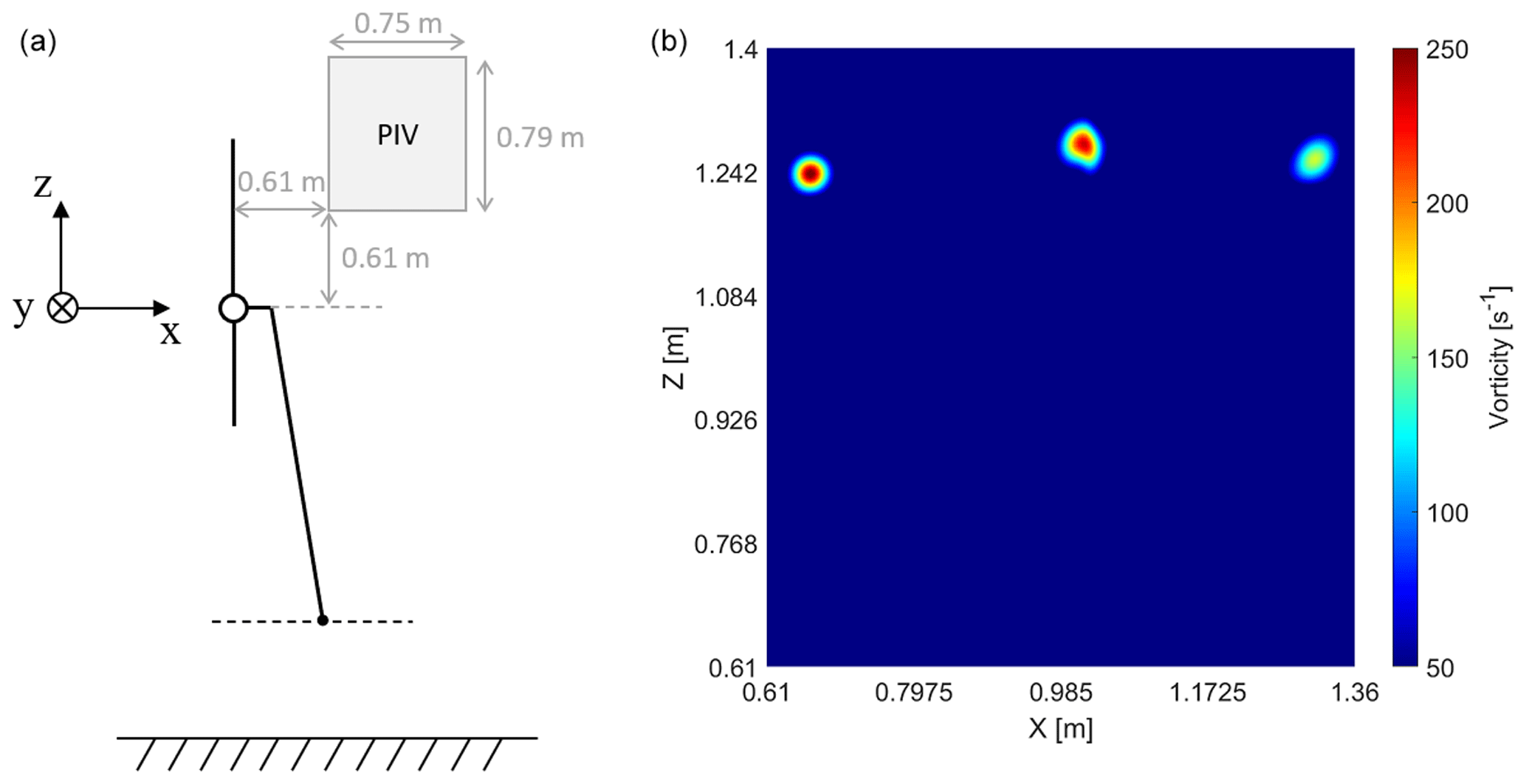
Figure 9 (a) Schematic representation of the wind turbine system and the PIV plane location. (b) Vorticity magnitude in the PIV plane during steady wind when the blade azimuth location is 30^∘.

5.1.3 PIV measurements

For Experiment 1, PIV measurements were taken during the steady wind condition. The longitudinal and vertical wind speeds as well as the vorticity magnitude of the y direction were recorded at locations from x=0.61 m to x=1.36 m and from z=0.61 m to z=1.4 m from the hub location with 5 mm increments in both directions. These velocity fields were measured at times determined by the azimuth angle of one of the blades. The blade azimuth angles of interest were from 0^∘ (blade pointing upwards) to 120^∘ with a 15^∘ step and from 120 to 360^∘ with a 30^∘ step. Figure 9a illustrates the location of this PIV plane behind the rotor. The location of this PIV plane can also be observed in Fig. 6. Figure 9b shows an example of vorticity magnitude measured in the PIV plane during the experiment when the reference blade is at 30^∘ azimuth position. For the older vortex downstream, a reduction in vorticity magnitude, as well as a less rounded shape due to the convection, diffusion, and stretching of the vortex, can be observed.

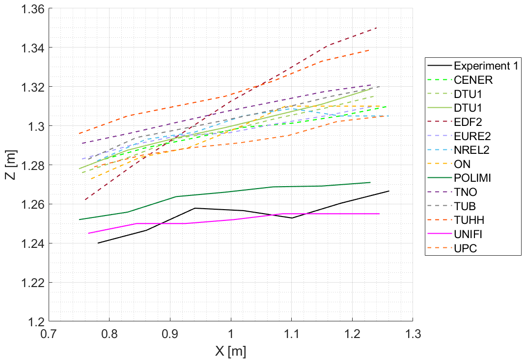
The scalar gamma 1 from Graftieaux's method (Graftieaux et al., 2001) was used for vortex tracking. Local maxima in the gamma 1 results were used to locate the centers of the blade-tip vortices (Soto-Valle et al., 2022). The PIV plane records blade-tip vortices from the three blades. Figure 10 shows the averaged blade-tip vortex trajectory for the experiment and the participants using FVW (dashed) and CFD (solid) within the PIV plane. As expected, the tip vortex trajectories move outboard with increasing vortex age (i.e., when vortices travel downwind). These tip vortex trajectories are representative of the wake expansion. Most numerical models tend to slightly overpredict the wake expansion. It is possible that the proximity of the blade tip to the ceiling in the experiments tends to inhibit a normal wake expansion (Soto-Valle et al., 2020). The CFD participants (e.g., POLIMI and UNIFI in Fig. 10) that included the wind tunnel walls, floor, and ceiling obtained a better agreement with the experiment. FVW participants cannot include this boundary condition in their numerical models without implementing additional features. Interestingly, DTU1 (CFD) did not include the wind tunnel ceiling, and the wake expansion is aligned with the behavior observed by most FVW participants. Cioni et al. (2023) also studied the hot-wire data and PIV data from Experiment 1 under steady and unsteady wind conditions and provided additional insights.

Figure 10 Averaged blade-tip vortex trajectory in the PIV plane during steady wind.

5.2 Unsteady wind

The unsteady inflow conditions were achieved by means of forced harmonic motions. The system was studied under the same incoming wind as the steady wind condition but included different platform motion frequencies ($\mathit{\omega }=\mathrm{2}\cdot \mathit{\pi }\cdot f$) and amplitudes (A). The platform displacement (x) is described according to Eq. (5), and the platform velocity ($\dot{x}$), stated by Eq. (6), is the time derivative of the platform displacement:

$$\begin{array}{}\text{(5)}& {\displaystyle }& {\displaystyle }x\left(t\right)=A\cdot \sin (\mathit{\omega }\cdot t)\text{(6)}& {\displaystyle }& {\displaystyle }\dot{x}\left(t\right)=\mathit{\omega }\cdot A\cdot \cos (\mathit{\omega }\cdot t).\end{array}$$

The apparent wind experienced by the rotor is described by Eq. (7), and it is the combination of the incoming wind (U₀) and the platform velocity:

$$\begin{array}{}\text{(7)}& w\left(t\right)=U_{\mathrm{0}}-\mathit{\omega }\cdot A\cdot \cos (\mathit{\omega }\cdot t).\end{array}$$

Figure 11 shows the platform displacement, platform velocity, and rotor apparent wind in the angle domain for one platform period. Instead of using time in the x axis, the platform-motion phase is used.

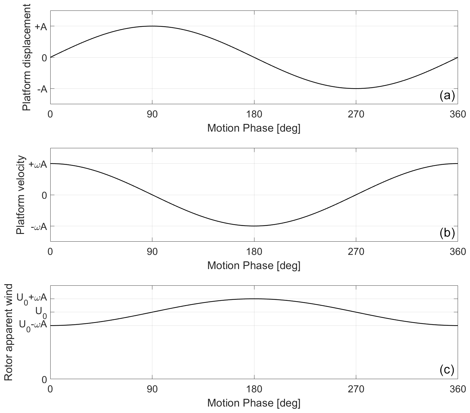
Figure 11 Platform displacement (a), platform velocity (b), and rotor apparent wind (c) during one platform period.

For the surge motion, some participants kept the platform fixed and provided the rotor apparent wind as input wind in their simulations. This is a valid approach for the surge test if the rotor does not move into and out of its own wake or if the numerical model does not account for this potential interaction. Most participants kept the wind speed fixed and forced the motion of the wind turbine.

The rotor loads (e.g., thrust force and torque) are expected to follow the rotor apparent wind behavior (Fig. 11c). Figure 12 shows the expected relationship between the rotor loads and the platform displacement. A phase shift of 90^∘ between the rotor loads and the platform displacement is expected for quasi-steady models. For example, BEM models with static polars should exhibit a phase shift of 90^∘.

Figure 12 Expected relationship between rotor loads and platform displacement.

5.3 Unsteady wind: Load Case 2.5

Load Case 2.5 experiences the largest rotor apparent wind variation for the surge motion. The rotor loads are clearly driven by the platform motion, which translates into a good signal-to-noise ratio in the experiments.

The measured rotor loads were low-pass filtered with a 3 Hz cutoff frequency, as mentioned in Sect. 4. This low-pass filter was performed in the frequency domain. The complex fast Fourier transform (FFT) was performed, the frequency of interest was kept (i.e., from 0 to 3 Hz), and the inverse of the FFT was applied to reconstruct the time domain signal. The main advantage of this approach is that it does not introduce a phase lag in the signal. For both experiments, the low-pass-filtered rotor loads include around 15 surge periods. The loads were binned according to the platform motion and phase averaged.

Figure 13 shows the aerodynamic thrust force from the two experiments and the participants. Different line styles are used to compare the different approaches. The participants using BEM are denoted with a dotted line, the ones using DBEM or GDW are denoted with a dashed–dotted line, the ones using FVW are denoted with a dashed line, and the ones using CFD are denoted with a solid line. In the legend, participants using different modeling approaches appear with the line style associated with their highest model fidelity used.

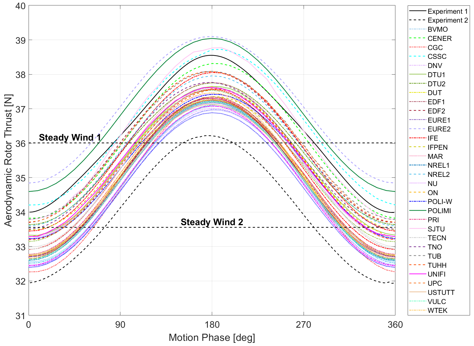
Figure 13 Aerodynamic rotor thrust variation during one surge period in Load Case 2.5. Results from the experiments and participants. Pattern: BEM (:), DBEM (-.), GDW (-.), FVW (- -), and CFD (–).

The experiments primarily exhibit a first-order sine wave. This indicates that the response is driven by a single frequency (the platform motion). Overall, the mean value for Experiment 1 and the participants is aligned with the value obtained during the steady case. For Experiment 2, there is a small offset that could be due to the zero blade pitch recalibration performed during the testing campaign. For reference, the steady wind values obtained during both experiments have been included in the plot by means of two horizontal dashed black lines.

Figure 14a shows the peak-to-peak amplitude of the aerodynamic rotor thrust. This peak-to-peak amplitude was computed as 2 times the FFT amplitude at the frequency of interest (e.g., 1 Hz corresponding to the platform motion in Load Case 2.5). Interestingly, the participants using the same code with BEM and DBEM (i.e., BVMO, EDF, EURE, NREL, TECN, and VULC) return very similar values. The maximum difference observed within each participant between accounting for or not accounting for dynamic inflow is 2.5 %. This indicates that the dynamic inflow does not have a significant impact in these conditions. Similarly, BEM or DBEM participants using the same code with static polars and unsteady airfoil aerodynamics (i.e., EDF, EURE, and NREL) show a maximum difference of 1 % in terms of peak-to-peak amplitude.

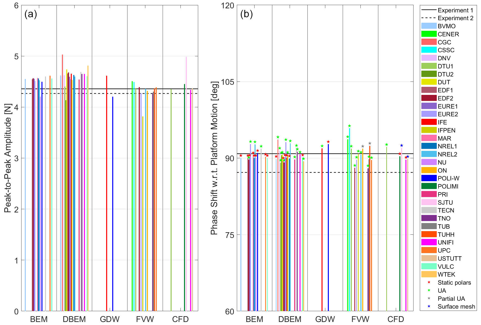
Figure 14 Aerodynamic rotor thrust peak-to-peak amplitude (a) and phase shift with regard to the platform motion (b) in Load Case 2.5.

Figure 14b shows the phase shift between the aerodynamic rotor load and the platform motion. The phase angle was computed based on the real and imaginary part of the complex FFT at the frequency of interest. A red star is included if the numerical model uses static polars, a green star denotes models accounting for unsteady airfoil aerodynamics (UA), and a blue star indicates models using surface mesh. For the FVW solutions, part of the flow hysteresis is already accounted for in the FVW theory. In this case, the solution is denoted as partial unsteady airfoil aerodynamics (gray star) if the participant used static polars. As anticipated in Fig. 12, the quasi-steady solutions (i.e., BEM with static polars) result in a phase shift at or very close to 90^∘. Most solutions including unsteady airfoil aerodynamics have phase shifts above 90^∘. This is due to a small hysteresis in airfoil performance undergoing angle of attack variations in attached flow (Theodorsen, 1935) rather than dynamic stall. The platform amplitudes and frequencies used in the experiment ensured that the dynamic stall was confined to the blade root (Fontanella et al., 2021b). The phase shift from most numerical models is aligned with the behavior observed in Experiment 1. Experiment 2 has a phase shift smaller than 90^∘ that could be due to the impact of small rotor speed variations during the testing.

Figure 15 shows the lift coefficient versus angle of attack of the blade radial station 7 (42 % blade span) for one surge period during Load Case 2.5. The output corresponds to two numerical models used by NREL with static polars (NREL1) and unsteady airfoil aerodynamics (NREL2). The static polar exhibits a constant slope as expected for the airfoil polar in the linear region; there is a unique relationship between the lift coefficient and the angle of attack. For the static polar, the lift coefficients when the platform moves from the 0 to 180^∘ phase are symmetric to the coefficients when the platform moves from the 180 to 360^∘ phase. This implies that the response must be symmetric around the 180^∘ motion phase if there is no other unsteadiness source (e.g., dynamic inflow). This symmetric behavior around 180^∘ can be observed for the quasi-steady solutions in Fig. 13. When unsteady airfoil aerodynamics are considered, the lift coefficient describes a hysteresis loop. As Fig. 15 shows, the lift coefficient when the platform moves from 0 to 180^∘ is smaller compared to when the platform moves from 180 to 360^∘. The response is not symmetric around the 180^∘ motion anymore, resulting in a phase shift in the rotor thrust slightly higher than 90^∘.

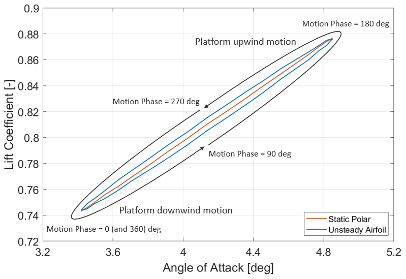
Figure 15 Lift coefficient versus angle of attack for a numerical model (NREL) using a lifting line with static polars or unsteady airfoil aerodynamics.

Figure 16 shows the summarized aerodynamic rotor thrust and torque during one surge period. The figure shows the median for each modeling approach and the phase-averaged behavior from both experiments. The subindex next to each modeling approach indicates the number of results. As can be observed, the aerodynamic rotor torque peak-to-peak amplitude in Experiment 2 is lower than in Experiment 1 (∼12 %). There are no significant differences in terms of peak-to-peak amplitude or phase lag between the numerical models. The most remarkable difference is in terms of the mean value for each modeling approach. In general, the mean value is consistent with the behavior observed during the steady wind condition (see Fig. 5 for reference). Only the CFD approach seems to exhibit a slightly different mean value compared to the steady wind condition. As Fig. 5 shows, the spread of the CFD participant outputs is significant. For Load Case 2.5, only five out of seven CFD participants reported results. This can impact the mean value observed in Load Case 2.5 compared to the steady wind condition.

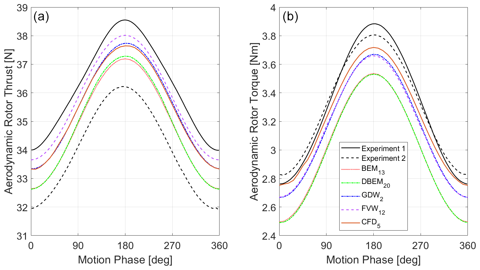
Figure 16 Aerodynamic rotor thrust (a) and torque (b) during the unsteady wind condition in Load Case 2.5.

5.4 Unsteady wind: platform motion summary

The same analysis provided in Sect. 5.3 was performed for the different surge and pitch motions. The platform pitch motion results in a skewed flow due to the rotor plane tilt angle. In this case, there are aerodynamic loads in different directions (e.g., F_x, F_y, F_z, M_x, M_y, M_z). However, the pitch amplitude is relatively small, and the amplitude of the loads different from the thrust and torque (i.e., F_y, F_z, M_y, M_z) are very small. To compare the different conditions, the peak-to-peak amplitude of the aerodynamic rotor loads (ΔF_x and ΔM_x) were normalized according to the platform motion amplitude (A) in meters.

Figure 17a shows the normalized aerodynamic rotor thrust variation for the different platform frequencies considered. The figure includes the results from both experiments and the median of the participants' results (simulation, all modeling approaches considered) for the platform surge and pitch motions. The figure also includes the results from Load Case 2.12 used for verification purposes.

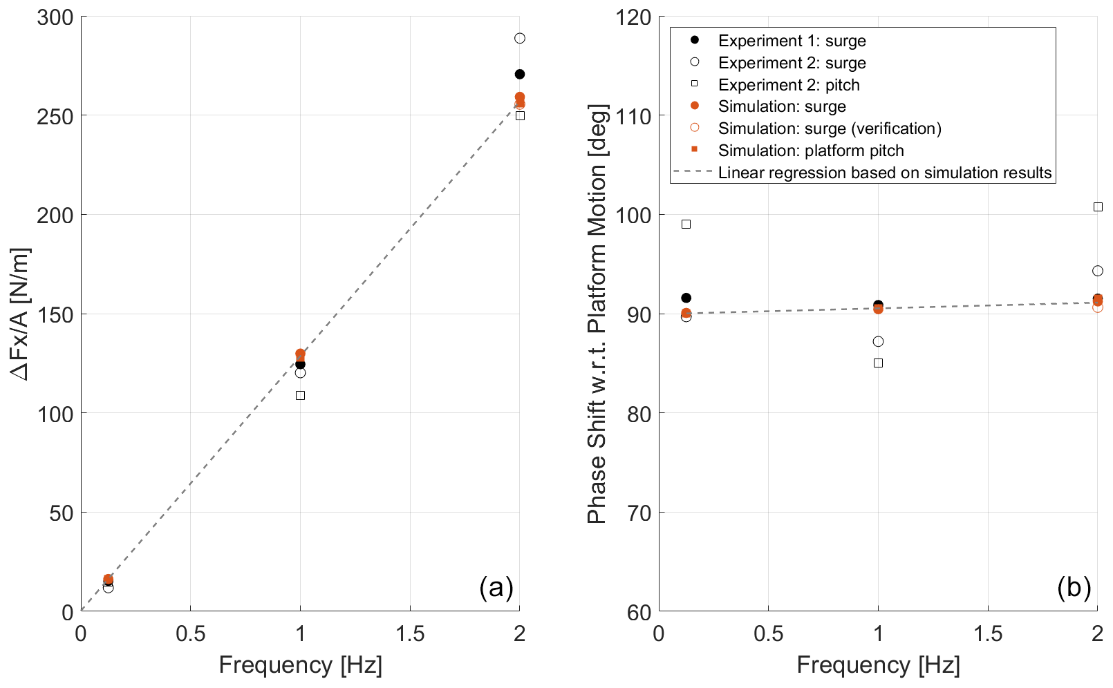
Figure 17 Normalized aerodynamic rotor thrust variation (a) and phase shift with regard to platform motion (b) during unsteady wind conditions using load cases from 2.1 to 3.7 (excluding Load Cases 2.16 and 2.17).

A linear regression was also fitted to the simulation results and included in Fig. 17. As can be observed, the simulation results lie on top of the linear regression for the frequency range studied. This confirms that the numerical models predict an aerodynamic rotor load variation that is linearly proportional to the changes in the rotor apparent wind, denoting a quasi-steady aerodynamic response. For example, increasing the platform motion amplitude or frequency by a factor of 2 would result in aerodynamic rotor load variations of the same order. This quasi-steady aerodynamic response is consistent with the behavior observed in previous studies (Mancini et al., 2020; Cormier et al., 2018). This behavior can also be verified by comparing the results from Load Case 2.7 and Load Case 2.12. These two load cases have the same platform frequency but different platform amplitudes. The platform amplitude in Load Case 2.12 was significantly increased from Load Case 2.7 to assess any potential unsteady aerodynamic response. When the aerodynamic rotor load is normalized by the platform amplitude, both load cases return the same value, confirming that there is no unsteady aerodynamic behavior. As expected, the linear regression shows zero variation in aerodynamic rotor loads at 0 Hz (i.e., no platform motion).

The agreement between the numerical models and the experiments is good at the frequencies of 0.125 and 1 Hz. No significant differences are observed between surge and the corresponding pitch motions. However, some spread is observed for the experiments at 2 Hz. This dispersion could come from the uncertainty associated with the inertial load subtraction from the measurements (Mancini et al., 2020).

Figure 17b shows the phase shift of the aerodynamic rotor thrust with respect to the platform motion. The numerical models predict a phase shift close to 90^∘ at low frequencies (quasi-steady behavior) and a small increase with the frequency. This is mainly due to the small hysteresis in the airfoil aerodynamics in the attached flow. The experiments show some dispersion, indicating that there is some uncertainty in the measurements. The results from Experiment 1 show the closest behavior in terms of aerodynamic thrust variation and phase compared to the numerical models.

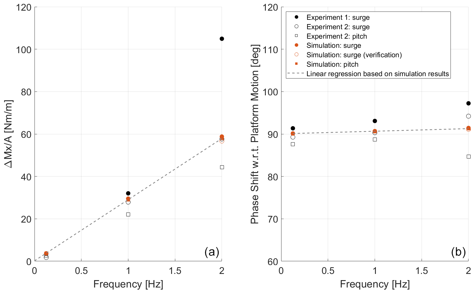
Figure 18 Normalized aerodynamic rotor torque variation and phase shift with regard to platform motion during unsteady wind conditions using load cases from 2.1 to 3.7 (excluding Load Cases 2.16 and 2.17).

Figure 18 shows equivalent information to Fig. 17 but in terms of aerodynamic rotor torque. Similar behavior as for the thrust force is observed. The main difference occurs in the aerodynamic torque variation at 2 Hz for Experiment 1. When looking at the frequency domain, the spectrum shows a significant amplitude at 2.5 Hz that could impact the system response during this testing condition, and therefore the results should be used cautiously. This issue was also reported in Mancini et al. (2020). This unexpected frequency is not observed during Experiment 2. For the aerodynamic rotor torque, the results from Experiment 2 (surge motion) show the closest behavior in terms of aerodynamic torque variation and phase compared to the numerical models.

5.5 Unsteady wind: rotor speed and blade pitch variations

During both experiments, the rotor speed and blade pitch angle were held constant. However, in real wind turbine operating conditions, platform surge and pitch variations would result in rotor speed variations and blade pitch actuations.

Modern variable-speed wind turbines use generator torque control and blade pitch angle control. Below rated power, the blades are kept at the minimum (optimal) blade pitch angle setting, and the wind turbine is governed by the generator torque. In this region, rotor torque changes due to unsteady wind conditions will lead to rotor speed variations. When the wind turbine is operating at rated power, the blade pitch angle is used to keep the wind turbine rotor at a constant speed and producing the desired power. In this region, the blade pitch angle needs to vary to keep the rotor torque constant. Near the rated power condition, the controller can be transitioning between the generator torque and blade pitch control. In this region, there could be rotor speed and blade pitch variations.

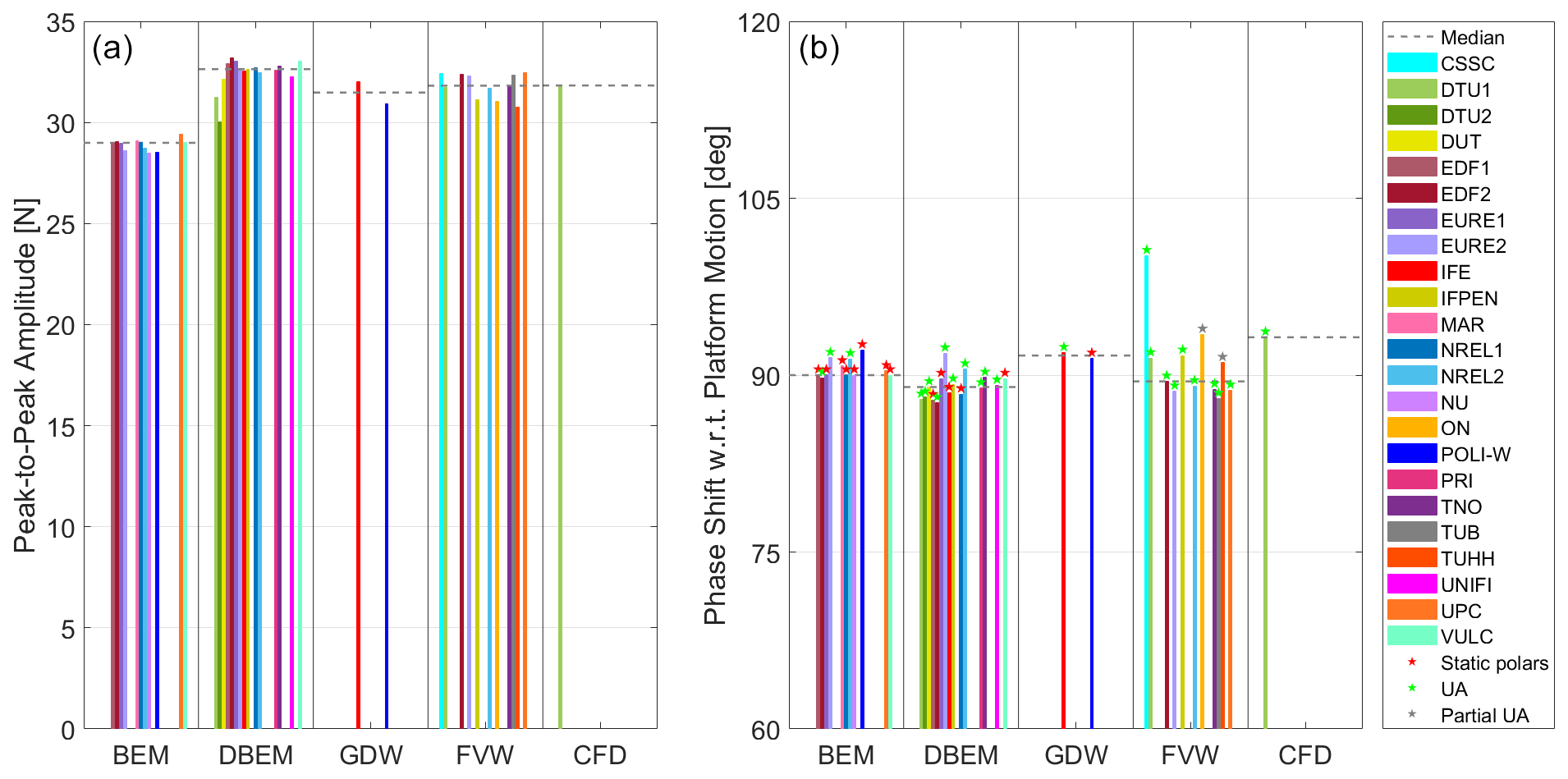
Figure 19 Aerodynamic rotor thrust peak-to-peak amplitude (a) and phase shift with regard to the platform motion (b) in Load Case 2.16.

To illustrate the impacts that the wind turbine controller could have on the system loading, verification load cases, 2.16 and 2.17, were included in the study (with no corresponding experimental measurements for validation). These two load cases use the platform motion from Load Case 2.12 as a baseline. The proposed rotor speed and blade pitch variations follow the same behavior as the aerodynamic rotor torque (i.e., they are governed by the rotor apparent wind). Equation (8) describes the rotor speed (Ω) in revolutions per minute in Load Case 2.16, and Eq. (9) describes the blade pitch angle (β) in degrees in Load Case 2.17. The proposed rotor speed and blade pitch variations are based on values observed in similar FOWT studies (Ramos-García et al., 2022). Under these conditions, the dynamic stall is confined to the blade root like for the previous load cases analyzed.

$$\begin{array}{}\text{(8)}& {\displaystyle }& {\displaystyle }\mathrm{\Omega }\left(t\right)=\mathrm{240}-\mathrm{36}\cdot \cos (\mathit{\omega }\cdot t)\left(\mathrm{Load}\mathrm{Case}\mathrm{2.16}\right)\text{(9)}& {\displaystyle }& {\displaystyle }\mathit{\beta }\left(t\right)=\mathrm{1.5}-\mathrm{1.5}\cdot \cos (\mathit{\omega }\cdot t)\left(\mathrm{Load}\mathrm{Case}\mathrm{2.17}\right)\end{array}$$

The rotor speed and blade pitch angle are imposed assuming that there are no system dynamics involved. In real conditions, the rotor would speed up or slow down at a rate that depends on the system rotational inertia and the generator-resistive torque curve. Regardless, the imposed motions should be reasonably representative.

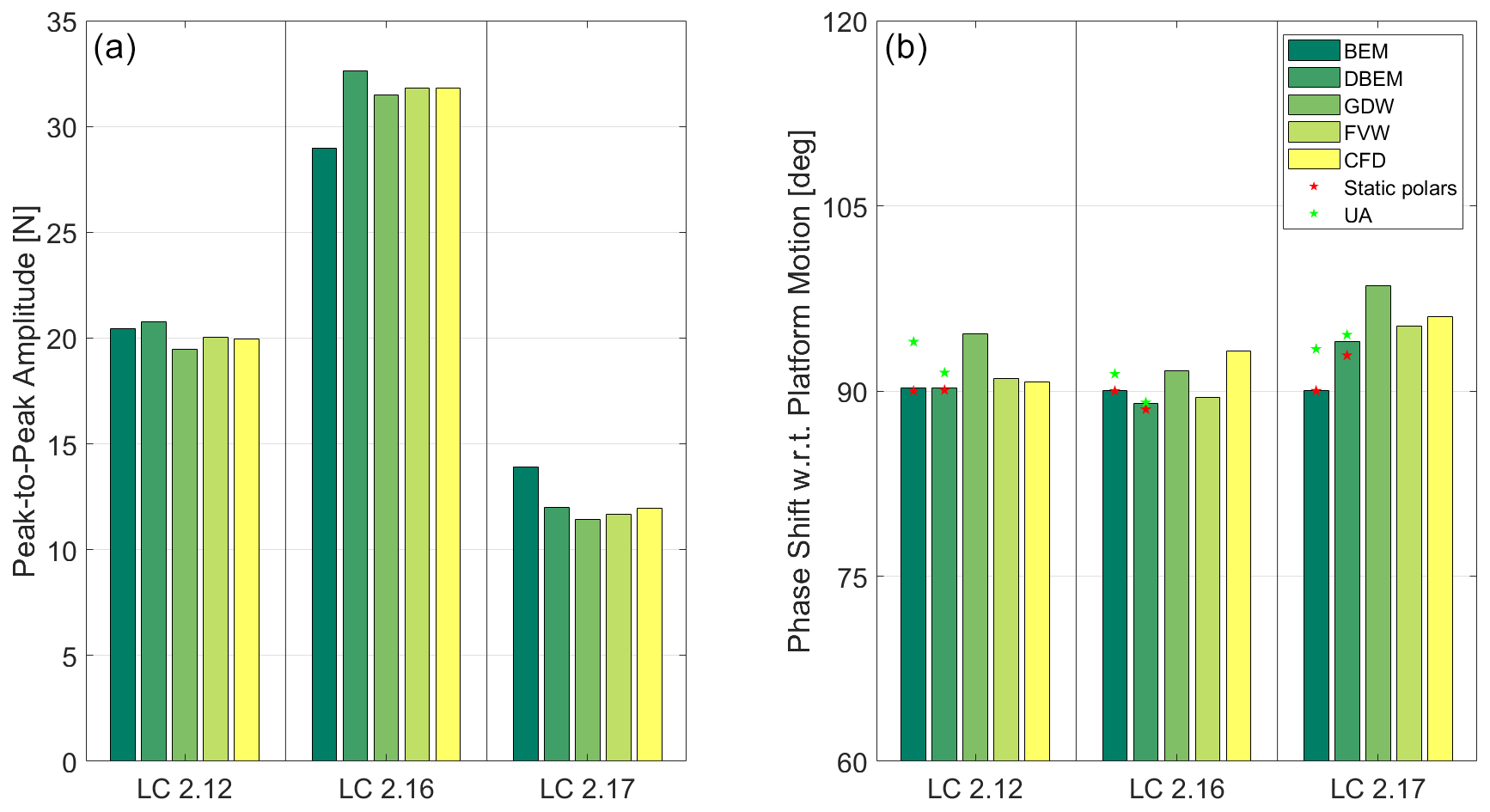
Figure 20 (a) Aerodynamic rotor thrust peak-to-peak amplitude in Load Case 2.12 (constant rotor speed and blade pitch), 2.16 (varying rotor speed), and 2.17 (varying blade pitch). (b) Phase shift with regard to the platform motion.

Figure 19a shows the aerodynamic rotor thrust peak-to-peak amplitude for the different participants and the median for each modeling approach in Load Case 2.16 (platform motion and rotor speed variation). Interestingly, the modeling approaches including dynamic inflow (DBEM, GDW, FVW, and CFD) predict similar values, while the BEM solution predicts a lower value. Figure 19b shows the phase shift with regard to the platform motion. Similar behavior is observed for the aerodynamic rotor torque (not shown).

Figure 20 shows a summary of the results of the modeling approach for Load Cases 2.12, 2.16, and 2.17. Figure 20a shows the aerodynamic rotor thrust peak-to-peak amplitude. For Load Case 2.16, the output is equivalent to the one shown in Fig. 19. The peak-to-peak amplitude in Load Case 2.16 is significantly larger than in Load Case 2.12 due to the rotor speed oscillations. The blade pitch actuation in Load Case 2.17 alleviates the rotor loading variations as intended by the wind turbine controller, resulting in smaller peak-to-peak amplitudes compared to Load Case 2.12.

There is a good agreement between modeling approaches when only the platform motion is considered (Load Case 2.12). The maximum difference between any approach and the average of all modeling approaches is within 3 %. However, when there is platform motion and rotor speed variations (Load Case 2.16), not accounting for dynamic inflow (i.e., BEM approach) results in load variation amplitudes that are 9 % lower compared to the average of the solutions that do account for dynamic inflow effects (DBEM, GDW, FVW, and CFD). When there is platform motion and blade pitch actuations (Load Case 2.17), not accounting for dynamic inflow results in load variation amplitudes that are 18 % higher.

The dynamic inflow effect for sudden blade pitch angle changes (e.g., step changes) is well known (Snel and Schepers, 1995). For sudden actuations, relevant dynamic overshoot loads compared to quasi-steady calculations are expected. Interestingly, for the blade pitch and platform harmonic motion considered here (Load Case 2.17), the dynamic inflow results in smaller peak-to-peak variations.

Figure 20b shows the phase shift of the aerodynamic thrust with regard to the platform motion by the modeling approaches. For the BEM and DBEM approaches, a red star denotes the median solution for the models using static polars, and a green star is used for the median solution of the models using unsteady airfoil aerodynamics. As expected, the BEM approaches with static polars show a phase shift of 90^∘ regardless of the operating conditions. The use of unsteady airfoil aerodynamics in BEM or DBEM returns phase shifts that are slightly higher compared to the static polars. The effect of the dynamic inflow in the phase shift can be observed in Load Cases 2.16 and 2.17. In Load Case 2.16, the phase shift slightly decreases compared to Load Case 2.12, while the phase shift in Load Case 2.17 slightly increases. Despite these variations, the phase shift remains close to the expected 90^∘ with a maximum difference smaller than 10^∘.

6 Conclusions

In the frame of the OC6 Phase III project, participants modeled a scaled version of the DTU 10 MW RWT and studied the system response under steady and unsteady wind conditions. The results of numerical models with different fidelity levels were compared against two testing campaigns, performed at Politecnico di Milano, for platform surge and pitch harmonic motions. A good agreement was observed between the numerical models and the experiments for the platform frequencies and amplitudes considered. For reference, these tests correspond to periods between 12.5 and 200 s at a full scale and nacelle motion amplitudes between 0.6 and 9.375 m. No significant differences between the numerical models of different fidelities were observed during the forced platform motions. For these tests, the aerodynamic rotor load was linearly proportional to the rotor apparent wind, denoting a quasi-steady aerodynamic response. Only a small hysteresis in airfoil performance undergoing angle of attack variations in attached flow was observed by participants using unsteady airfoil aerodynamics. This introduced a small phase shift in the rotor loads, but the impact was limited.

Additional load cases were also included to understand if other conditions could produce a significant unsteady aerodynamic behavior. It was observed that the change in the flow conditions due to rotor speed and blade pitch variations combined with the platform motion resulted in such an unsteady aerodynamic response. While there were no measurement data available for these conditions, the numerical models showed significant differences based on the modeling approach used. Those that did not include dynamic inflow effects predicted rotor load variation amplitudes 9 % smaller under rotor speed variations and load variation amplitudes 18 % higher when there were blade pitch actuations. The dynamic inflow also had a limited impact on the phase of the rotor loads. Thus, this work has shown that while the motion of the turbine itself does not require an unsteady aerodynamic modeling approach to accurately predict the loads in the turbine (at least for the design and forced motion studied in this project), a realistic condition where generator torque control and blade pitch angle control are included will need unsteady aerodynamic models (both airfoil unsteady aerodynamics and dynamic inflow models) for accurate load prediction.