Nonlinear inviscid aerodynamics of a wind turbine rotor in surge, sway, and yaw motions using a free-wake panel method

We investigate the aerodynamics of a surging, heaving, and yawing wind turbine with numerical simulations based on a free-wake panel method. We focus on the UNAFLOW (UNsteady Aerodynamics of FLOating Wind turbines) case: a surging wind turbine which was modeled experimentally and with various numerical methods. Good agreement with experimental data is observed for amplitude and phase of the thrust with surge motion. We achieve numerical results of a wind turbine wake that accurately reproduce experimentally verified effects of surging motion. We then extend our simulations beyond the frequency range of the UNAFLOW experiments and reach results that do not follow a quasi-steady response for surge. Finally, simulations are done with the turbine in yaw and heave motion, and the impact of the wake motion on the blade thrust is examined. Our work seeks to contribute a different method to the pool of results for the UNAFLOW case while extending the analysis to conditions that have not been simulated before and providing insights into nonlinear aerodynamic effects of wind turbine motion.

1 Introduction

With the wind energy market leaning heavily towards offshore turbines in recent years, floating offshore wind turbines (FOWTs) have become the focus of numerous research groups. One of the many challenges of such configurations is that, due to oceanic waves, the turbine is subjected to large amplitude motions, making its aerodynamics even more complex than that of onshore turbines. Turbines can translate horizontally perpendicular (surge) or parallel (sway) to the rotor plane. They can translate vertically (heave). They can rotate around the tower axis (yaw) or around the two horizontal axes (roll and pitch). These degrees of freedom are illustrated in Fig. 1.

The sway and heave motion are, from a rotor aerodynamics perspective, equivalent. Rolling moves the rotor in a very similar way to sway, with an added in-plane rotation, equivalent to a change in rotation velocity. Pitching can be thought of as a combination of surge, yaw, and heave. Hence, for rotor aerodynamics, we can consider the surge, yaw, and sway as the fundamental forms of rotor motion from which the others can be derived. For this reason, in this study, we focus on these three degrees of freedom. While these rotor motions have been studied experimentally (Fontanella et al., 2022), the frequencies and amplitudes of the motion are typically limited, and inertial effects can affect the accuracy of the results. Hence, numerical studies are needed to investigate FOWT motion.

The UNAFLOW (UNsteady Aerodynamics of FLOating Wind turbines; Bayati et al., 2018b; Fontanella et al., 2021a) project provided a simplified test case for a non-stationary rotor by simulating a surging wind turbine in a wind tunnel without any tilting of the tower. Several groups have simulated the UNAFLOW case with different methodologies including blade element momentum theory (BEM), lifting line, and computational fluid dynamics (CFD), with fairly good results being achieved (Bayati et al., 2018a; Boorsma and Caboni, 2020; Cormier et al., 2018). Furthermore, vortex methods have shown promising results for FOWTs in surge and other degrees of freedom for other turbines (Ramos-García et al., 2022b, a).

Figure 1 Degrees of freedom of a FOWT.

While BEM simulations have successfully captured dynamic inflow conditions (Mancini et al., 2023), most of the research has focused on dynamic blade pitch, streamwise velocity fluctuations, or surge. Recent developments have been made to extend BEM to general wind turbine motion (Mancini et al., 2022), but, to our knowledge, validation of these models for sway conditions has not been extensive. Dynamic yaw and sway motion have the potential to be more difficult to capture than surge, as the wake moves from side to side and the assumptions of momentum theory may lead to large errors.

This work is an expansion of what was documented in a previous conference publication (Ribeiro et al., 2022b). For a full description of the numerical methods, along with verification and validation with relevant cases, refer to that paper. Here, we seek to contribute to the pool of UNAFLOW results by simulating the UNAFLOW case with a source and doublet free-wake panel method. Unlike BEM and lifting line, panel methods directly model the blades, free from table look-ups, while still being a fraction of the cost of a CFD simulation (Leishman, 2002). Blade thickness effects are included by simulating the entire blade surface rather than the camber surface or a single line, which can lead to better accuracy (Yang et al., 2020). Panel methods have also been shown to accurately model full rotors, including aeroelastic effects (Gennaretti et al., 2018; Sessarego et al., 2015; Wang et al., 2016). The free wake allows for complex scenarios, such as blade–vortex interaction (Gennaretti and Bernardini, 2007), which could happen in extreme surge conditions.

With these characteristics in mind, this is an important stepping stone towards the ultimate goal of this research: aeroelastic simulations of FOWTs through a fully coupled transient aerodynamic and structural fluid–structure interaction (FSI). To our knowledge, only experimental and CFD results have been used to investigate the wake of the UNAFLOW turbine (Bayati et al., 2018a). CFD adds significant diffusion to the tip vortices, making comparisons to experiments difficult. Hence, in this work we also show how the free-wake panel method compares to experimental measurements of the wake.

The next objective of this work is to extend the surge analysis to sway and yaw motion. We use the UNAFLOW rotor to perform such investigations in order to contribute to the knowledge of the physics of these motions. Finally, we seek to understand the impact of the wake motion on surge, sway, and yaw. We do this by employing unique features of the free-wake panel method, allowing us to include rotor motion effects indirectly. The analysis of wake motion effects seeks to clarify mechanisms of turbine motion that will need to be accounted for when simulating FOWT motion with methods without true wake motion, such as BEM and prescribed wake vortex methods.

2 Methodology

We employ a source and doublet panel method with free wakes (Katz and Plotkin, 2001) in order to capture the aerodynamics of the surging wind turbine rotor. The thickness effects are fully captured, as the panels lie on the blades' surfaces. Blade–vortex interaction capabilities (Gennaretti and Bernardini, 2007) are implemented but not used for this study, as the turbine does not cross its own wake. The surface and wake discretization of the velocity potential equation leads to the following linear system:

$$\begin{array}{}\text{(1)}& {\displaystyle \frac{\mathrm{1}}{\mathrm{4}\mathit{\pi }}}{A}_{ij}{\mathit{\mu }}_j+{\displaystyle \frac{\mathrm{1}}{\mathrm{4}\mathit{\pi }}}{B}_{ij}{\mathit{\sigma }}_j+{\displaystyle \frac{\mathrm{1}}{\mathrm{4}\mathit{\pi }}}{C}_{iw}{\mathit{\gamma }}_w=\mathrm{0},\end{array}$$

where A, B, and C are the influence coefficient matrices (Maskew, 1987) for the doublets μ, sources σ, and wake vortices γ, respectively. The values of μ, σ, and γ are constant over each panel. The sources σ are computed to ensure impermeability, the wake vortices γ enforce the Kutta condition (Youngren et al., 1983), and the doublets μ are the unknowns. At every time step, wake vortices are convected due to the freestream velocity and the induction of all the surface and wake panels.

When symmetries are present, as in turbines with multiple blades and no yaw or heave, virtual bodies across symmetry planes or axes can be used (Katz and Plotkin, 2001), which dramatically reduce the influence coefficient matrices. With the linear system solved, surface velocities U are computed based on the basic potential flow equation, $\mathit{U}=-\mathrm{\nabla }\mathrm{\Phi }$, where Φ is the velocity potential. The surface gradient is computed with central differences for quadrangular panels, but a least squares approximation (Anderson and Bonhaus, 1994; Sozer et al., 2014) is also available and is always used for triangular panels. With the surface velocity available, the unsteady Bernoulli equation (Bernardini et al., 2013) is used to find the surface pressure, which is then integrated over all surface panels to find the forces and moments acting on the bodies. The time derivative in the unsteady Bernoulli equation is calculated with a first-order backwards Euler method.

The panel method shown here was created with the intent to be faster than available methods through the use of efficient algorithms and modern acceleration techniques, such as leveraging GPUs for the calculations. At the moment, our implementation was compared to an open-source C++ panel code (Baayen, 2012), and we observed speedup of over an order of magnitude. The method also supports large displacement aeroelasticity (Ribeiro et al., 2022a), although this is not included in this work.

3 Surging wind turbine simulations

The UNAFLOW turbine case (Fontanella et al., 2021a) consists of a three-blade rotor with a diameter of 2.38 m, rotating at 150 to 265 rpm, with U_∞ between 2.5 and 6 m s⁻¹. The entire rotor surges upwind and downwind at a frequency (f) ranging from 0.125 to 2 Hz and amplitude (A) from 2.5 to 125 mm, with the rotor center axial position following Asin (2πft), where t is time. In non-dimensional terms, for the case with U_∞=4 m s⁻¹, this corresponds to reduced frequencies $f_{\mathrm{r}}=fD/U_{\mathrm{\infty }}$ between 0.07 and 1.2 and normalized amplitude $A_{\mathrm{r}}=A/D$ between 0.001 and 0.05. This motion is performed such that the rotation axis is always aligned with the freestream, meaning no yawed flow occurs. As the majority of the experimental data are for U_∞=4 m s⁻¹ and revolutions per minute of 241, these are the conditions we simulate in this work. We use different values of f and A for our simulations, based on the availability of experimental data, while giving a preference to cases with high surge velocity U_S=2πfA. For details on full-scale values for these quantities, see Ribeiro et al. (2022b).

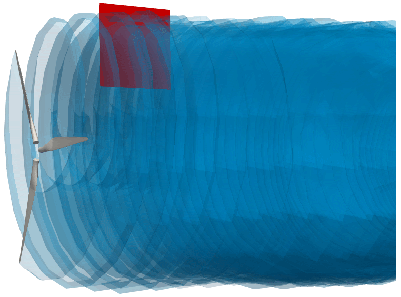
The blades are based on the SD7032 airfoil section, transitioning into a circle in the root region. For the simulations in this work, the blade geometry was constructed based on chord and twist distributions provided in the experimental data set (Fontanella et al., 2021b). However, this led to small differences in the geometry. In particular, the blade chord approaches zero at the tip (Bayati et al., 2016), which is inconsistent with the geometry description (Fontanella et al., 2021b) and can lead to some differences in results. Figure 2 shows the UNAFLOW wind turbine, along with its wake, as simulated by the methods described in this paper. The blades are simulated without the hub and tower for simplicity.

Figure 2 Panel method simulation results of the UNAFLOW rotor and its wake.

The blades are discretized with 100 chordwise panels, using a cosine distribution, and 50 equally spaced spanwise panels each, with a total of about 15 000 panels. The panel distribution is shown in Fig. 3. This panel distribution was chosen as it provided grid converged results for several preliminary studies on airfoils and rotors, not included here for brevity. The blade tips and roots are closed to enforce impermeability. Wake panels are only shed from the trailing edges, meaning no vorticity can be shed from the 90^∘ edges at the tips and roots. The time step is set to $\mathrm{1}/\mathrm{36}$ of a revolution unless otherwise stated, which corresponds to a rotation angle of $\mathrm{\Delta }\mathit{\psi }=\mathrm{10}{}^{\circ }$. Simulations are run for at least 40 revolutions, leading to about 216 000 wake panels. This time discretization corresponds to 72 time steps per surging period for f=2 Hz, which is the highest surge frequency available in the experimental data set.

Figure 3 Surface mesh used for the UNAFLOW blade, showing tip region.

For a demonstration of the accuracy of the chosen time steps, simulation duration, and validation of the mean flow properties, refer to Ribeiro et al. (2022b). Here, we focus on the main results for surge while normalizing the plots in a different way than in the original publication, as this will help with comparisons to the other rotor motions. The main parameter we will use throughout this work is the thrust coefficient C_T:

$$\begin{array}{}\text{(2)}& C_{\mathrm{T}}={\displaystyle \frac{T}{\frac{\mathrm{1}}{\mathrm{2}}\mathit{\rho }\mathit{\pi }{R}^{\mathrm{2}}{U}_{\mathrm{\infty }}^{\mathrm{2}}}},\end{array}$$

where T is the thrust force, ρ is the air density, and R is the turbine radius.

3.1 Surge velocity effects

We examine the fluctuating component of C_T while keeping A=15 mm (A_r=0.006) and varying f between 0 and 2 Hz (f_r between 0 and 1.2). Figure 4 shows the effect of f_r on the amplitude of the fluctuations in thrust (ΔC_T), normalized by A_r. Note that ΔC_T is the amplitude that would multiply a sine function to represent the time history of C_T, or $(C_{\text{Tmax}}-C_{\text{Tmin}})/\mathrm{2}$, assuming a time history of C_T that is perfectly sinusoidal. Figure 5 shows the effect of f_r on the phase shift ϕ between the rotor position and the fluctuations in C_T. The experimental data shown throughout this paper were filtered at the surge frequency. The lowest surge frequency, f_r=0.3 Hz, was run for twice as long as other cases to obtain meaningful statistics from the simulations.

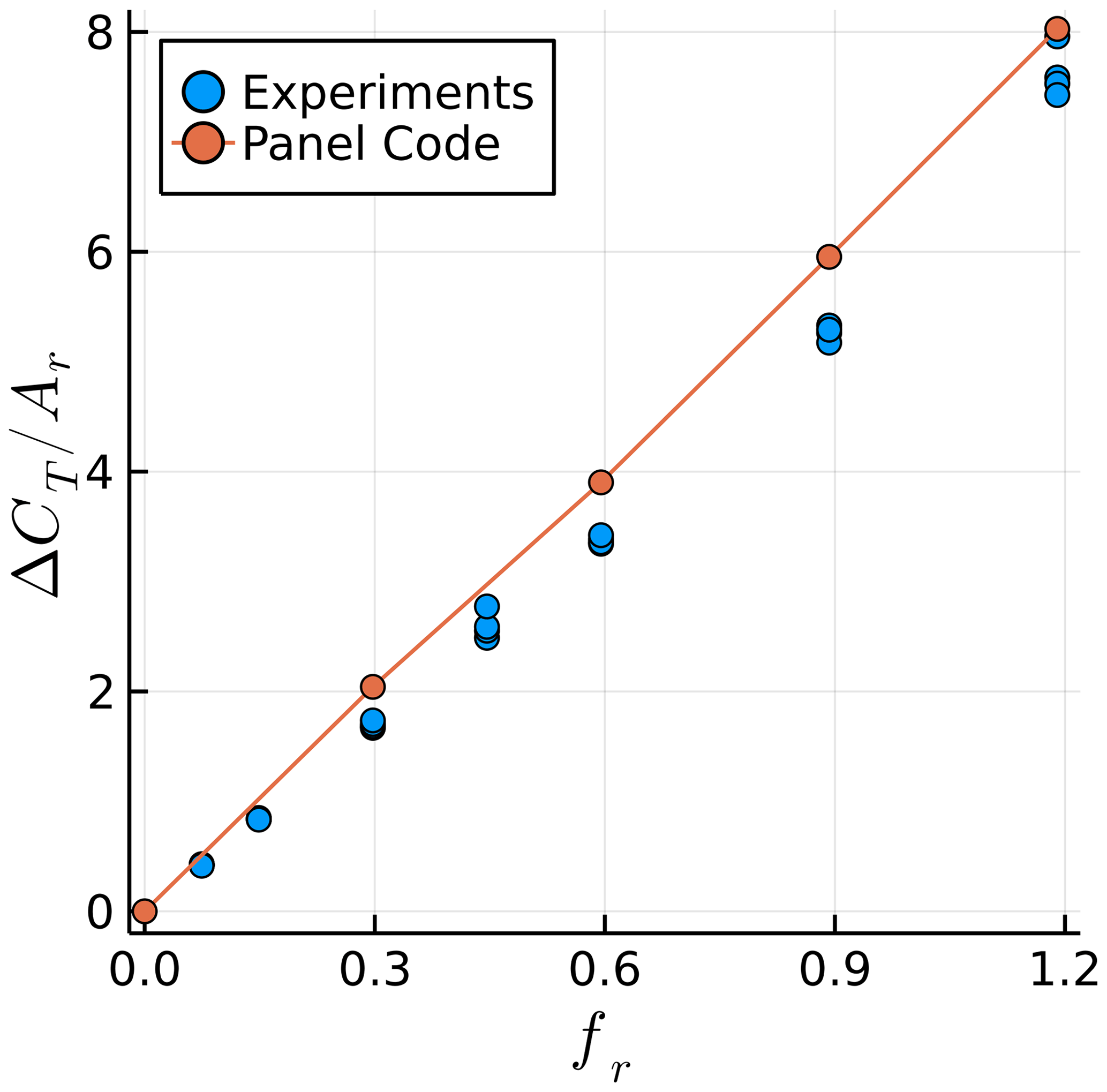
Figure 4 Surge frequency effect on the amplitude of the fluctuation in the thrust coefficient. Simulations at constant A and experiments at various A are shown.

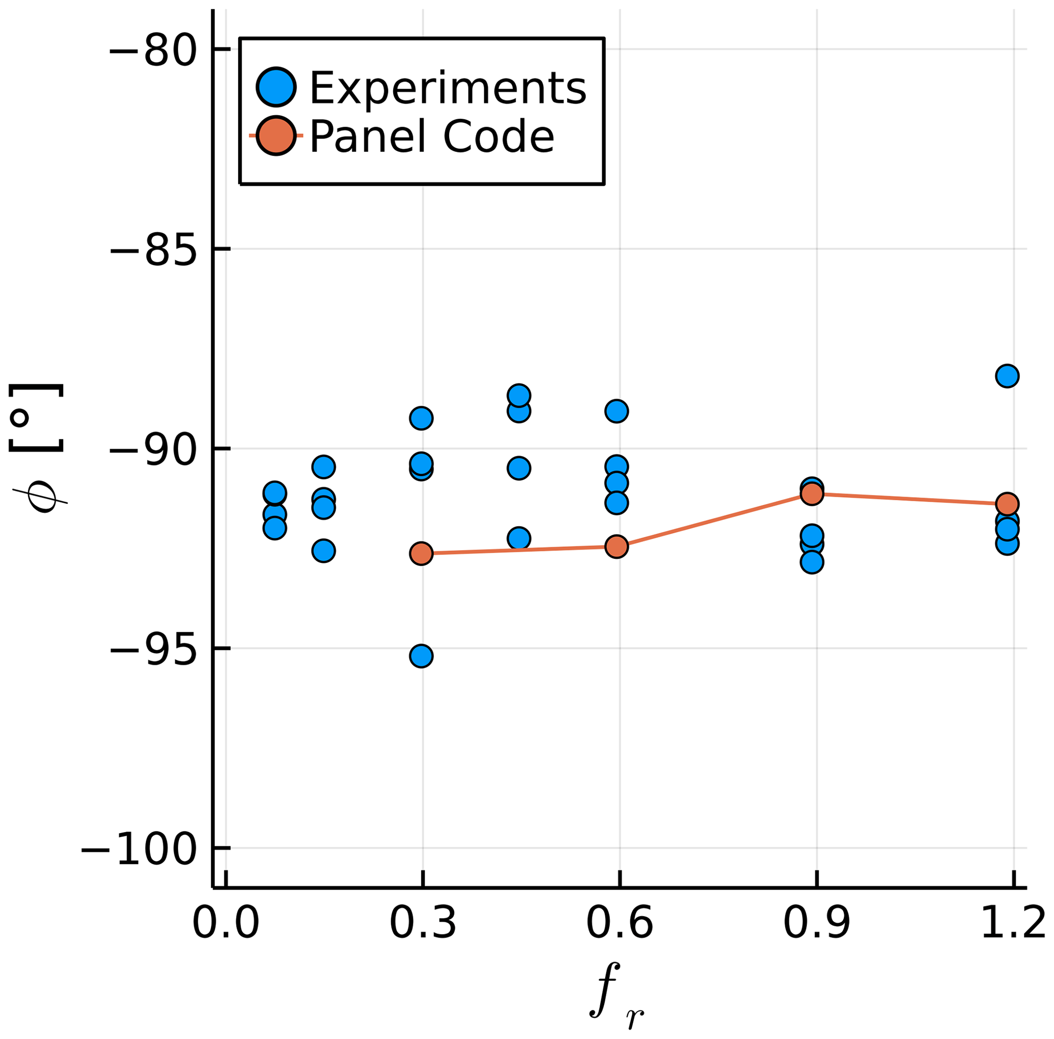
Figure 5 Surge frequency effect on the phase between the rotor position and its thrust. Simulations at constant A and experiments at various A are shown.

The values of $\mathrm{\Delta }{C}_{\mathrm{T}}/A_{\mathrm{r}}$ agree well with experimental data, with an approximately linear relation between the surge velocity and the thrust fluctuations. This confirms the quasi-steady nature of the results, which is likely due to the relatively small values of U_S (Mancini et al., 2020). The average slope of $\mathrm{\Delta }{C}_{\mathrm{T}}/A_{\mathrm{r}}$ as a function of f_r in the simulations is 15 % higher than in the experiments likely due to the inviscid approach. The values of ϕ fall within the experimental scatter, being within 3^∘ of −90^∘ for all cases, which corresponds to the quasi-steady response.

3.2 Rotor wake

We now focus on the rotor wake. The UNAFLOW experiments included particle image velocimetry (PIV) on a vertical plane in the rotor wake, aligned with the center of the nacelle. Measurements were made at several stages of the surging motion and averaged over several snapshots, with the rotor always being in the same azimuth (Fontanella et al., 2021a). We focus on two rotor positions, which the experiments refer to as steps 1 and 5. Both steps correspond to the rotor being in its central position (x=0), with the rotor moving with maximum velocity against the wind in step 1 ($\dot{x}=-U_{\mathrm{S}}$) and maximum velocity with the wind in step 5 ($\dot{x}=U_{\mathrm{S}}$). As the rotor is in the same position and same azimuth for both steps, any change in the wake is caused by unsteady effects of the surging motion.

Simulations are done with f=1 Hz and A=35 mm, which correspond to f_r=0.6, A_r=0.015, and $U_{\mathrm{S}}/U_{\mathrm{\infty }}=\mathrm{0.055}$. This configuration was selected since it contains PIV data for all steps while also having a high value of U_S. Figure 6 shows the UNAFLOW rotor, along with the wake panels and the PIV plane, as a reference for the results discussed in the following paragraphs. When the rotor crosses steps 1 and 5, the bottom blade is rotated 187^∘ away from the PIV plane.

Figure 6 UNAFLOW wind turbine (grey), wake panels (blue), and PIV plane (red).

Figures 7 and 8 show experimental and numerical results on the PIV plane. Both steps 1 and 5 are shown in each figure in order to better see the difference between them. The precise location of the tip vortices in the simulation is highlighted as pink points in both figures for comparisons. Consistent with expectations, during step 1 the tip vortices are further downstream than in step 5. The horizontal distance between the vortices in steps 1 and 5 is very well captured by the simulation, being about 6 cm in both simulations and experiments. The vortices' radial and streamwise positions are noticeably different between simulations and experiments likely in large part due to the blades' tip geometry not being identical to the experimental blades, as they are not described in detail in the documentation. The blades in the simulations are slightly longer and have a larger chord on the tip. It should be noted that the PIV data indicate the wake is shrinking in radius, which should not be the case and is likely an effect of experimental uncertainty. The expanding wake in the simulations is more realistic.

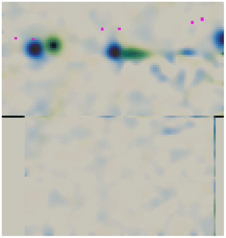
Figure 7 Experimental tip vortices' position on steps 1 (green) and 5 (blue). Vorticity perpendicular to the plane shown from 0 to 300 1$/$s. Pink dots represent the tip vortices from the panel method simulation.

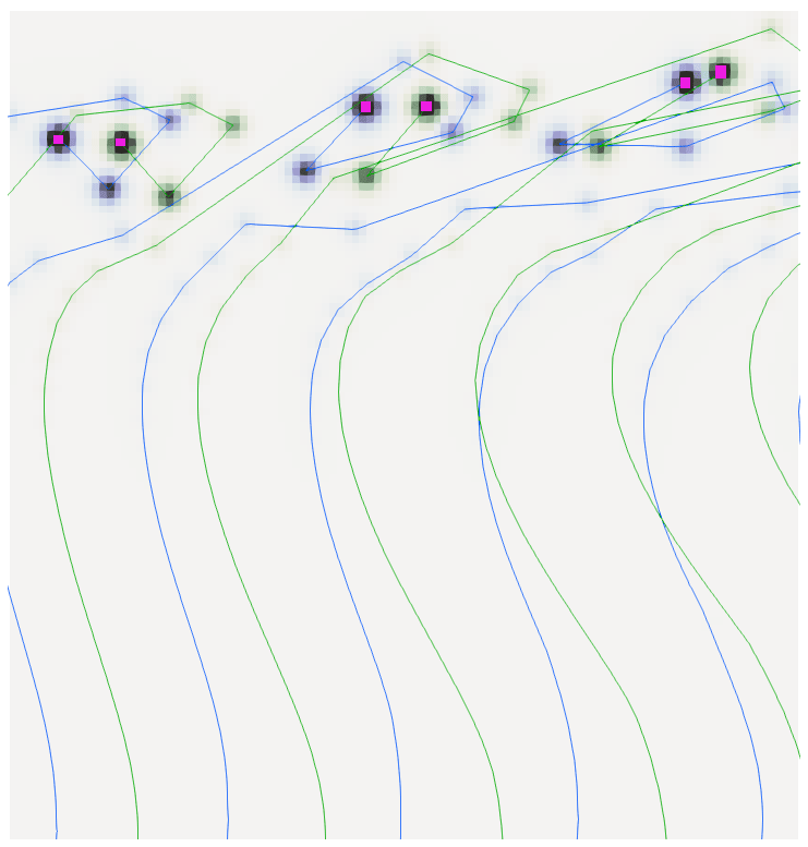
Figure 8 Numerical wake on steps 1 (green) and 5 (blue). Vorticity perpendicular to the plane shown from 0 to 300 1$/$s. Lines represent a cut through the wake panels. Pink dots highlight the tip vortices.

CFD simulations conducted for the UNAFLOW turbine (Bayati et al., 2018a) were able to capture the horizontal displacement of the first tip vortex in Figs. 7 and 8 to some extent. However, the second tip vortex displacement was inverted; that is to say that the vortex from step 1 was upstream of the position in step 5. To our knowledge, no other studies have been made where the wake of a surging wind turbine was simulated numerically and the results were validated with experiments. Hence, we believe this is the first time that a surging wind turbine simulation shows results that agree well with experimental data in terms of wake dynamics.

It is worth noting that the wind turbine wake is folding upon itself on the right side of Fig. 8. This is a common consequence of using an inviscid free-wake method, as complex wakes tend to become tangled as they develop, which can be partially observed on the right side of Fig. 2. Using a vortex core model (Ramasamy and Leishman, 2007) can stabilize the wake for a longer time if the vortex core radius is large enough but has small effects on the location of the tip vortices in the plane investigated here. The simulations shown here employed the aforementioned vortex core model and achieved better wake stability with it. Without a vortex core model, the wakes became entangled at earlier locations.

3.3 Beyond the UNAFLOW results

In this section, we seek to expand our simulations beyond the limitations of the UNAFLOW experiments. Due to the relatively small reduced frequencies involved in wind turbine surge motion (Tran and Kim, 2016) and the assumptions of inviscid flow in the simulations, we do not expect superlinear increases in ΔC_T. Based on Theodorsen (Theodorsen, 1934) results on airfoil sections, we expect first to see nonlinear behavior in the phase and then a sublinear change in ΔC_T. For more details, see Ribeiro et al. (2022b).

Results for simulations beyond the experimental data are shown in Figs. 9 and 10. The orange circles represent the data shown in Sect. 3.1, with A=0.015 mm and f varying between 0.5 and 2 Hz. The green circles show an extension of the orange data, with the same A but with f varying from 2 to 8 Hz. The dashed grey line in Fig. 9 is a linear extension of the orange circles. The grey region in Fig. 10 represents the quasi-steady regime, which we set around −90 ± 3^∘, as this contains most of the experimental data.

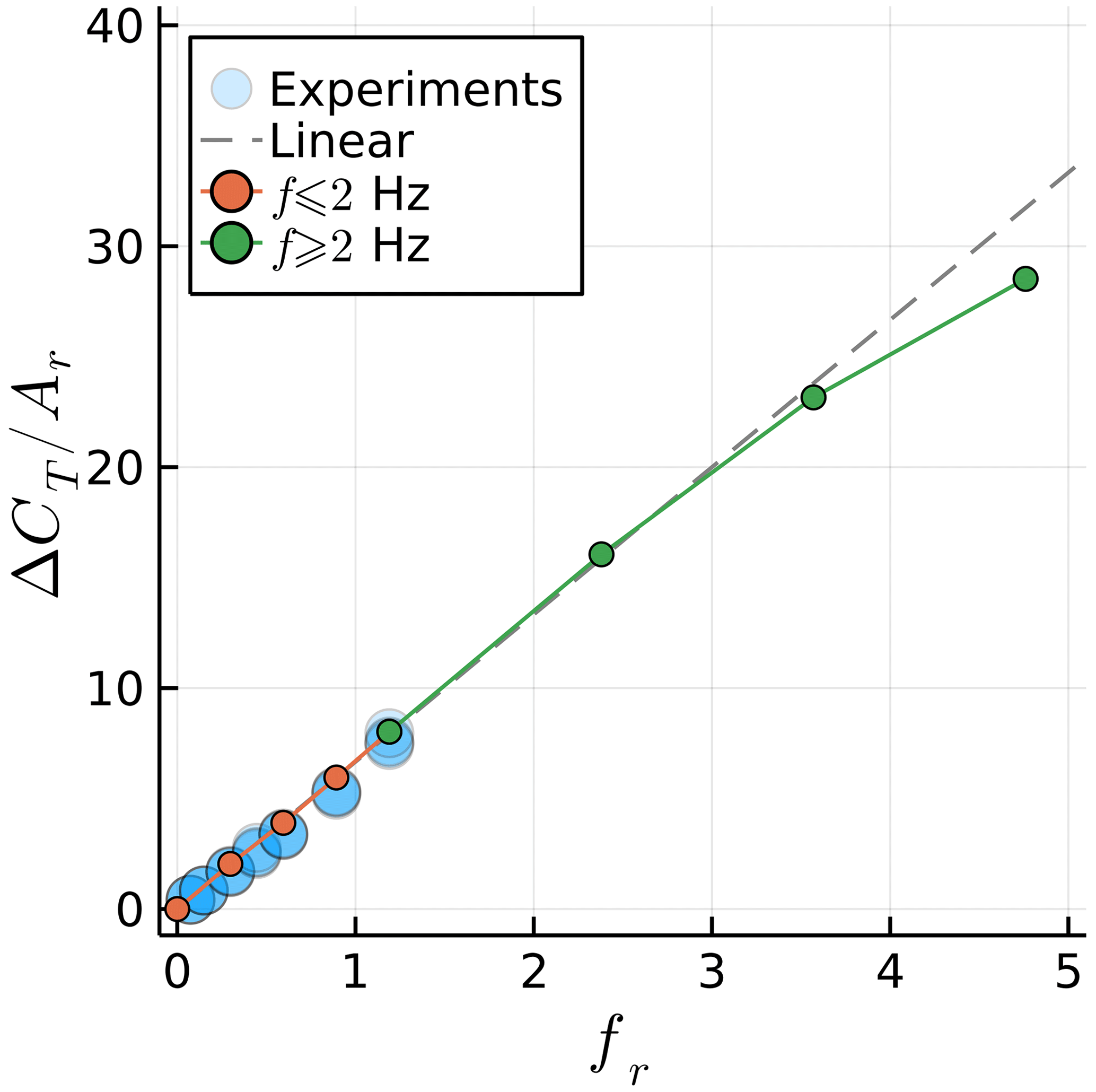
Figure 9 Maximum surge velocity effect on the amplitude of the fluctuation in the thrust coefficient.

Figure 10 Maximum surge velocity effect on the phase between the rotor position and its thrust.

We can now find where $\mathrm{\Delta }{C}_{\mathrm{T}}/A_{\mathrm{r}}$ breaks from a linear trend and when ϕ leaves the quasi-steady regime. At f_r=3.6, we observe a noticeable deviation from the linear relation between $\mathrm{\Delta }{C}_{\mathrm{T}}/A_{\mathrm{r}}$ and f_r. Increasing f_r leads to a reduction in ΔC_T instead of the increase seen in 2D. In contrast ϕ moves away from the quasi-steady regime at an earlier point, near f_r=2.

Normalizing ΔC_T with the surge amplitude and plotting results against the frequency is sufficient to collapse the experimental data here, as demonstrated in previous studies. For a discussion on how to normalize surging rotor data, see Mancini et al. (2020). However, the normalization used herein for f_r might not be sufficient to collapse nonlinear data with different flow conditions. If the nonlinear effects occur due to Theodorsen effects as is the case here, the rotor revolutions per minute should likely be taken into account, as it is an important factor for the value of k along the blades.

4 Swaying and yawing wind turbine simulations

We now move on to simulations of the two other degrees of freedom of interest for FOWTs in this work: sway and yaw. We continue to use the UNAFLOW turbine in spite of no experimental data being available for the cases investigated in this section. Although not shown, some of the simulations in Sect. 3 used symmetry conditions, with only a single blade of the rotor being simulated. This is no longer possible, as the introduction of lateral wind makes the loads on the blades asymmetric. Hence, all simulations in this section include all three blades.

4.1 Fixed turbine with side wind

In order to identify the dynamic effects of sway and yaw, we first need to understand the static effects of side wind. Hence, we simulate a fixed UNAFLOW rotor with side wind. This is usually referred to as a yaw case, but to avoid confusion between static and dynamic yaw cases, we refer to the static yaw cases as side wind throughout this paper and use the word “yaw” to refer to dynamic rotation around the tower axis.

We perform side wind simulations by rotating the wind vector around the vertical axis by a side slip angle β varying between 0 and 40^∘ (see Fig. 11). Even though this is a static simulation, results can not converge to a steady state, as the blades experience different wind vectors during a rotation, making cases with side slip intrinsically unsteady. However, as there are three blades, the dynamic loads on the blades mostly cancel each other out, leading to negligible fluctuations in rotor thrust. This occurred in our simulations for side wind, sway, and yaw. Hence, instead of investigating C_T on the entire rotor, we instead look at it on a single blade, or C_Tb. This value becomes periodic as the simulation progresses, and its fluctuation amplitude ΔC_Tb will be investigated in this and the following sections.

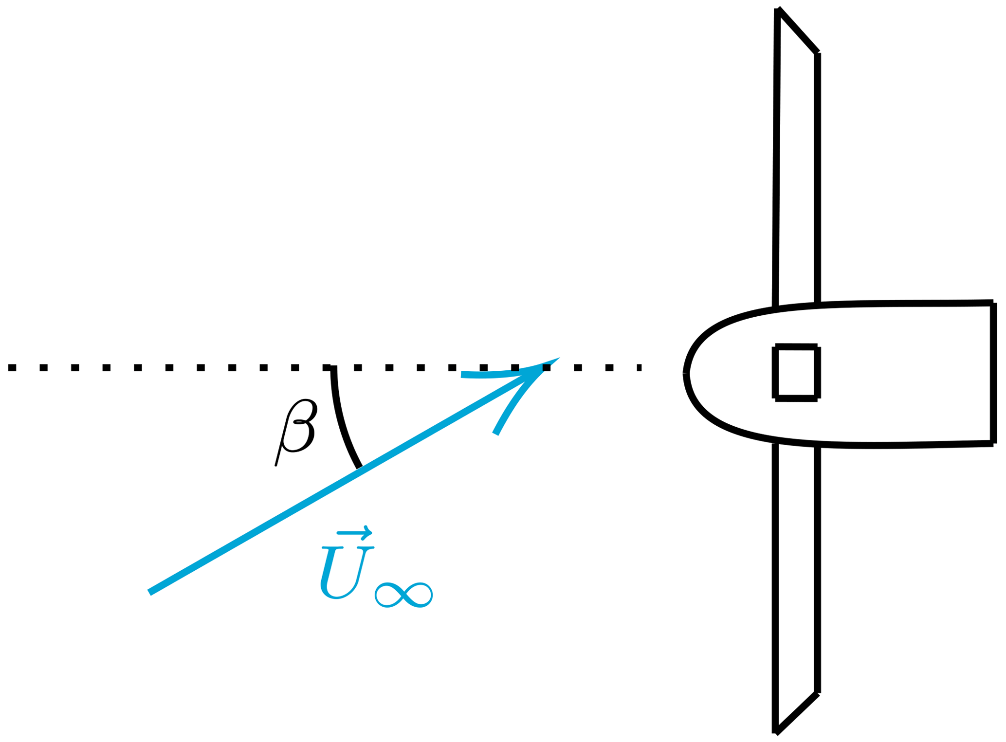
Figure 11 Top view of turbine with definition of side slip angle β. Dotted line represents the rotor axis.

Figure 12 shows the effect of β on ΔC_Tb. We see a linear trend, with the thrust fluctuations increasing as β increases up to about 10^∘. After that, the results are nonlinear and, as in surge, fall below the linear trend. For the high values of β we investigate here, flow separations would likely occur in real turbines, increasing C_Tb. We highlight that for side wind, C_Tb varies periodically as a sine wave with the frequency of the rotor rotation. This serves as a baseline for the results that follow.

Figure 12 Axial force fluctuation amplitude of single blade during rotation for different side wind angles.

4.2 Swaying turbine

We impose a swaying motion on the turbine using the same conventions of Sect. 3. We set A_r=0.05 and conduct simulations at f between 1 and 5 Hz. Again we use ΔC_Tb to measure the sensitivity of the blades to the unsteady loads. In this and the next sections, we start the rotor motion with one blade pointing straight up and refer to this as “blade 1”. The other blades are numbered in clockwise direction, looking downwind. The choice of the blade can affect the results, as will be shown.

The sway motion introduces a side velocity, which at its maximum value V_S=2πfA (when the rotor is at the center of the motion) introduces a maximum side wind angle ${\mathit{\beta }}_{\text{max}}={\tan }^{-\mathrm{1}}(V_{\mathrm{S}}/U_{\mathrm{\infty }})$ (see Fig. 13). We can use β_max to compare the sway results to the static results of the previous section. Note that the sway velocity adds to U_∞, meaning C_Tb must be scaled with a higher incoming velocity or multiplied by cos (β_max)² for a fair comparison with the side wind case, which we do.

Figure 13 Top view of turbine with definition of maximum side wind angle β_max.

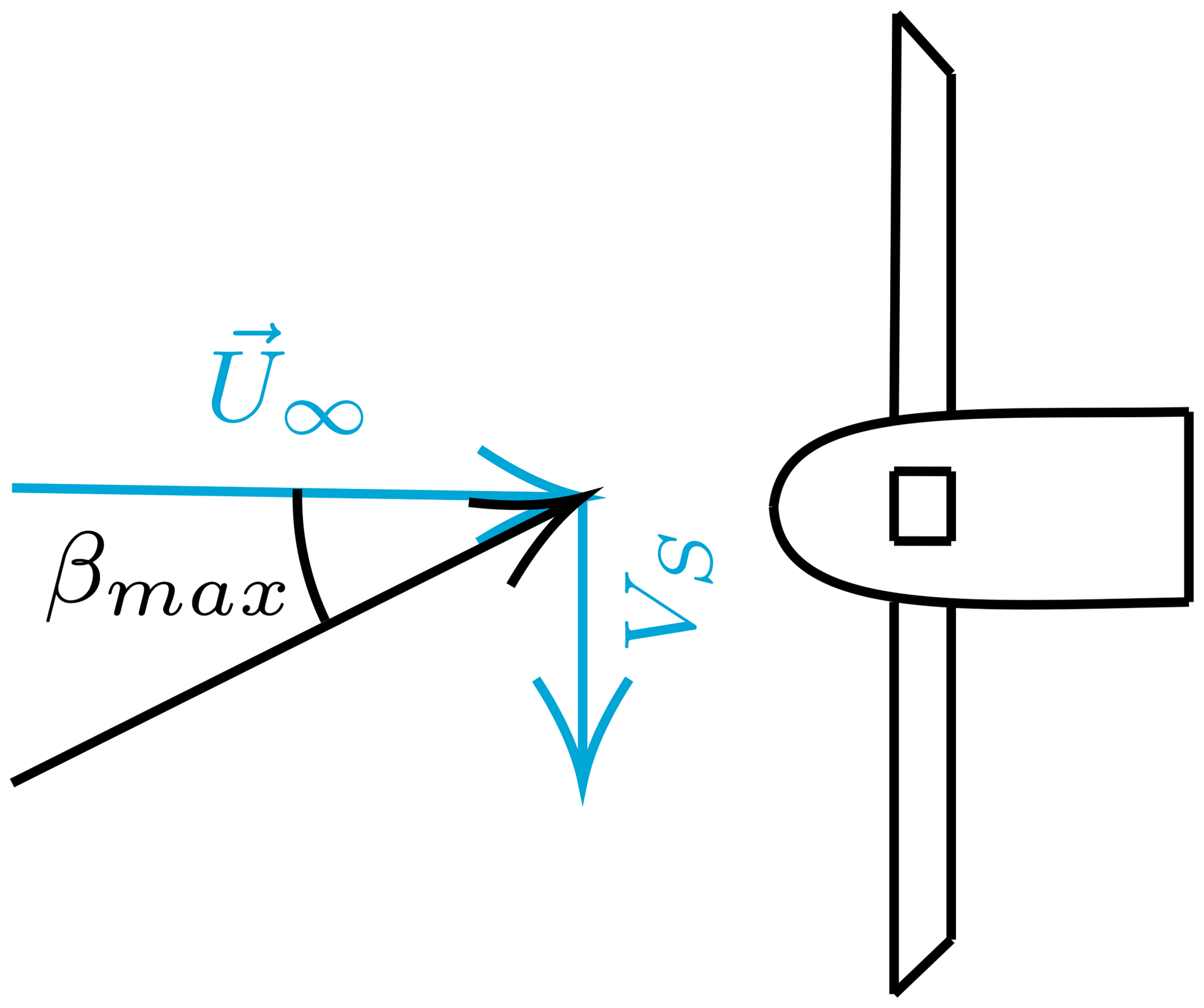
Figure 14 shows the time history of C_Tb for blade 1 at different values of f. The signals repeat periodically, and we show one period for clarity. The mean values of C_Tb reduce with frequency due to the scaling explained in the previous paragraph. The forces on the blades actually increase with f. We see that, unlike the surge and side wind results, more than one frequency is involved in the response to sway motion. Figure 15 shows the amplitude of each sway frequency as a function of the maximum β experienced during sway, along with the side wind results of the previous section. The effects become nonlinear for values of β_max similar to those seen in the side wind results. A substantial discontinuity appears for ${\mathit{\beta }}_{\text{max}}=\mathrm{40}{}^{\circ }$, where f is equal to the rotation frequency, making the response in Fig. 14 a simple sine wave and reducing ΔC_Tb.

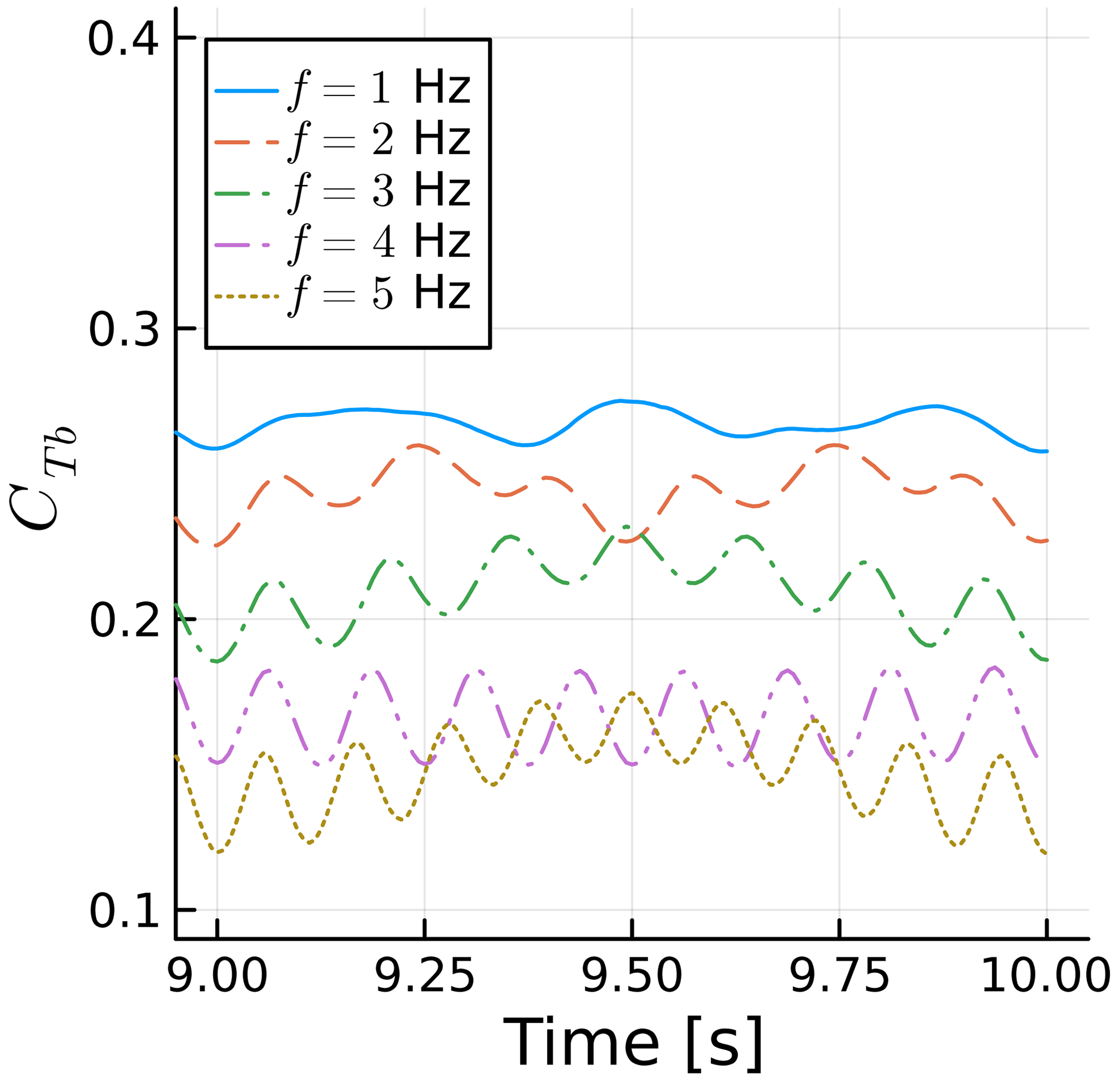
Figure 14 Time history of blade 1 thrust coefficient for various sway frequencies. Thrust normalized with maximum rotor velocity magnitude.

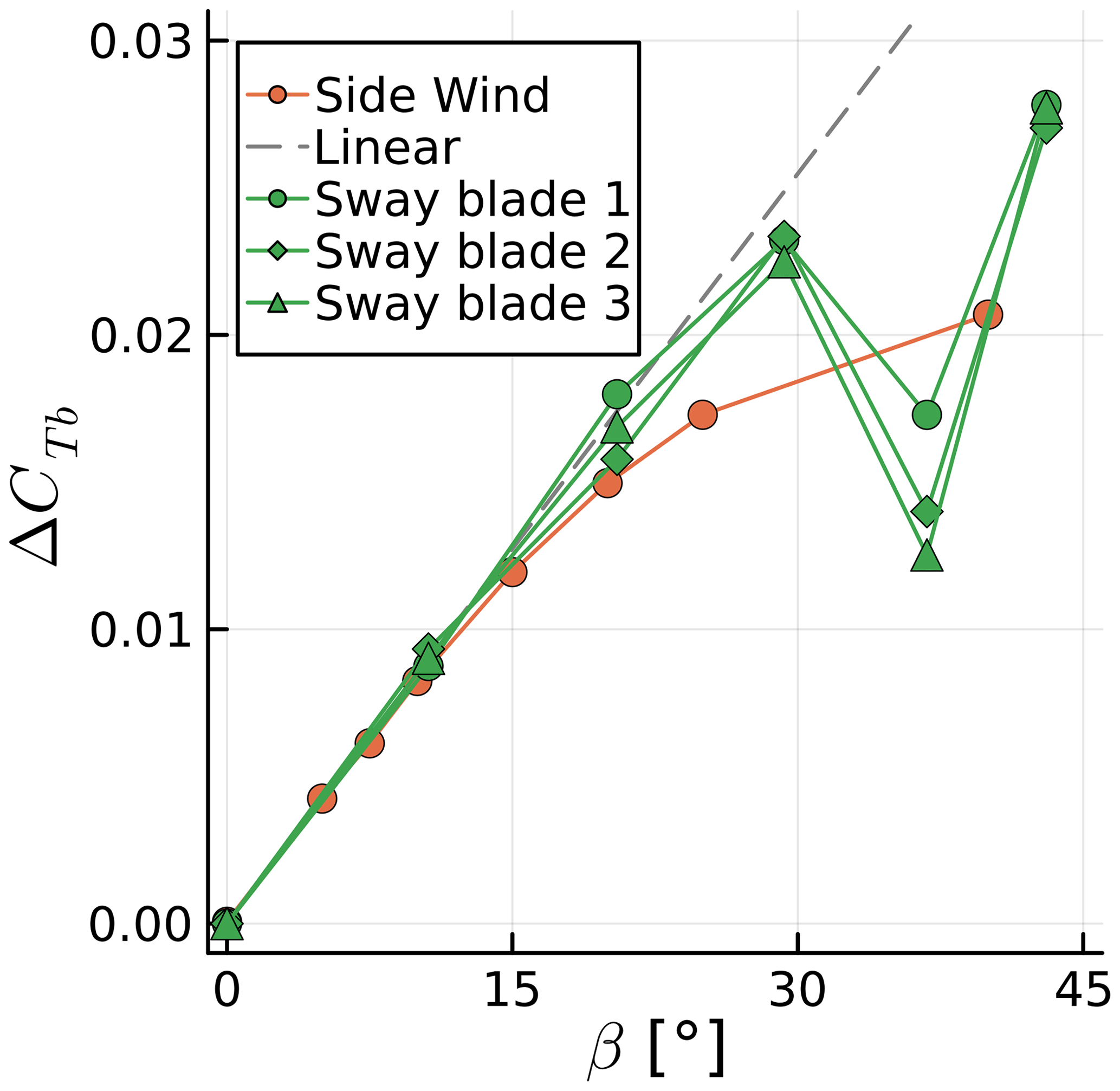
Figure 15 Amplitude of blade thrust coefficient fluctuation for various side wind angles and various maximum side wind angles achieved during sway motion. Thrust normalized with maximum rotor velocity magnitude.

By scaling ΔC_Tb with cos (β_max)², we are able to match the linear regions of the sway cases with the side wind results. Note that without this scaling, ΔC_Tb grows in a superlinear fashion instead of the sublinear trend seen in Fig. 15. Different studies may or may not include such a factor, which would potentially lead to conflicting conclusions.

We now take a closer look at one of the curves of Fig. 14 to explain their behavior. We take the case at f=2 Hz because it is relatively simple due to its sway frequency being half of the rotation frequency but complex enough that it can serve as an example to explain all the other curves. Figure 16 shows a zoomed in view of C_Tb as a function of time, where the blade azimuth is shown as vertical lines. Figure 17 shows the horizontal rotor sway velocity projected onto the blade chord V_S,c in the same intervals and with the same vertical lines. The color conventions for the azimuth ψ are shown in Fig. 18.

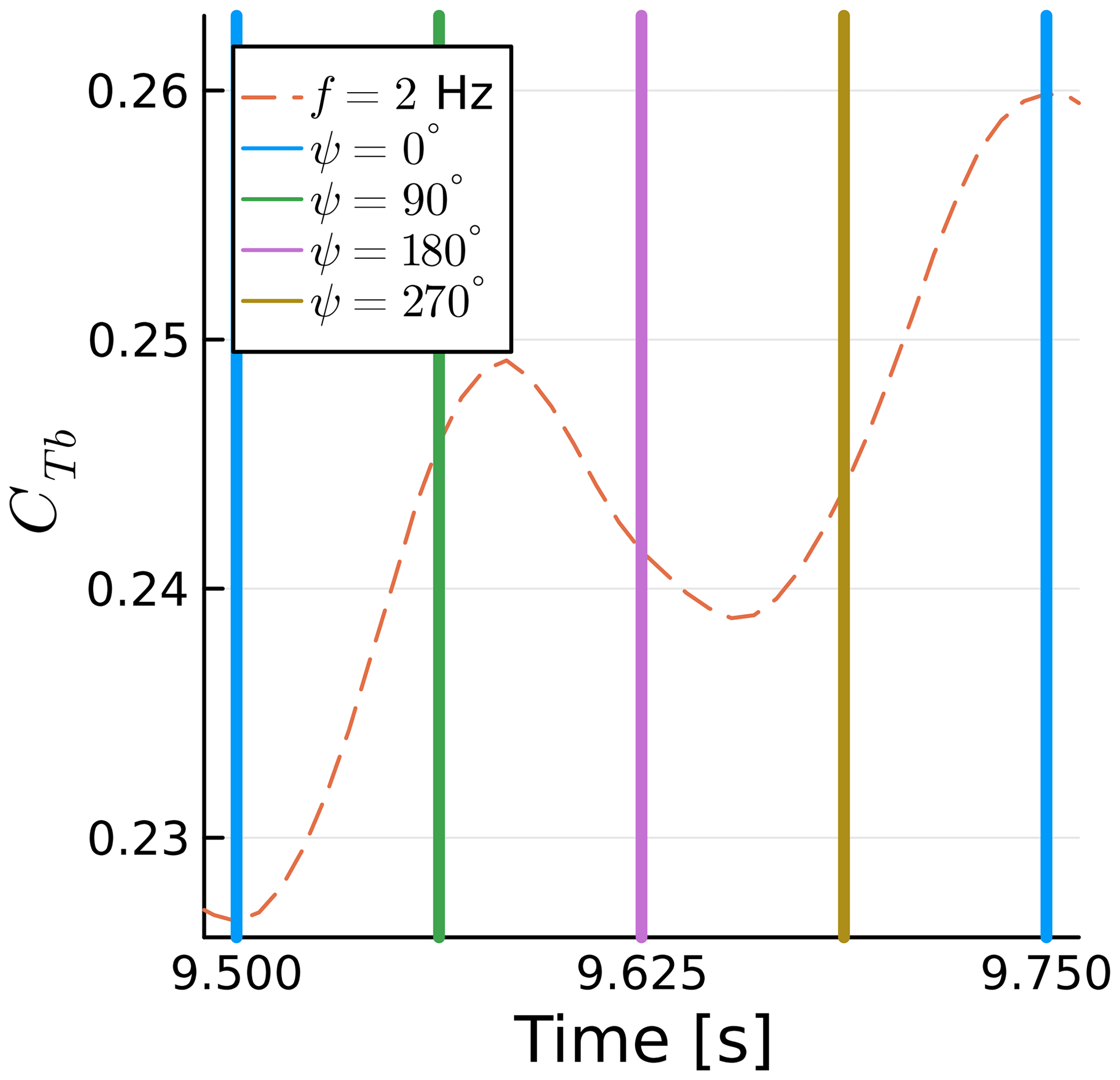
Figure 16 Time history of blade 1 thrust coefficient for a sway case. Vertical lines show blade azimuth.

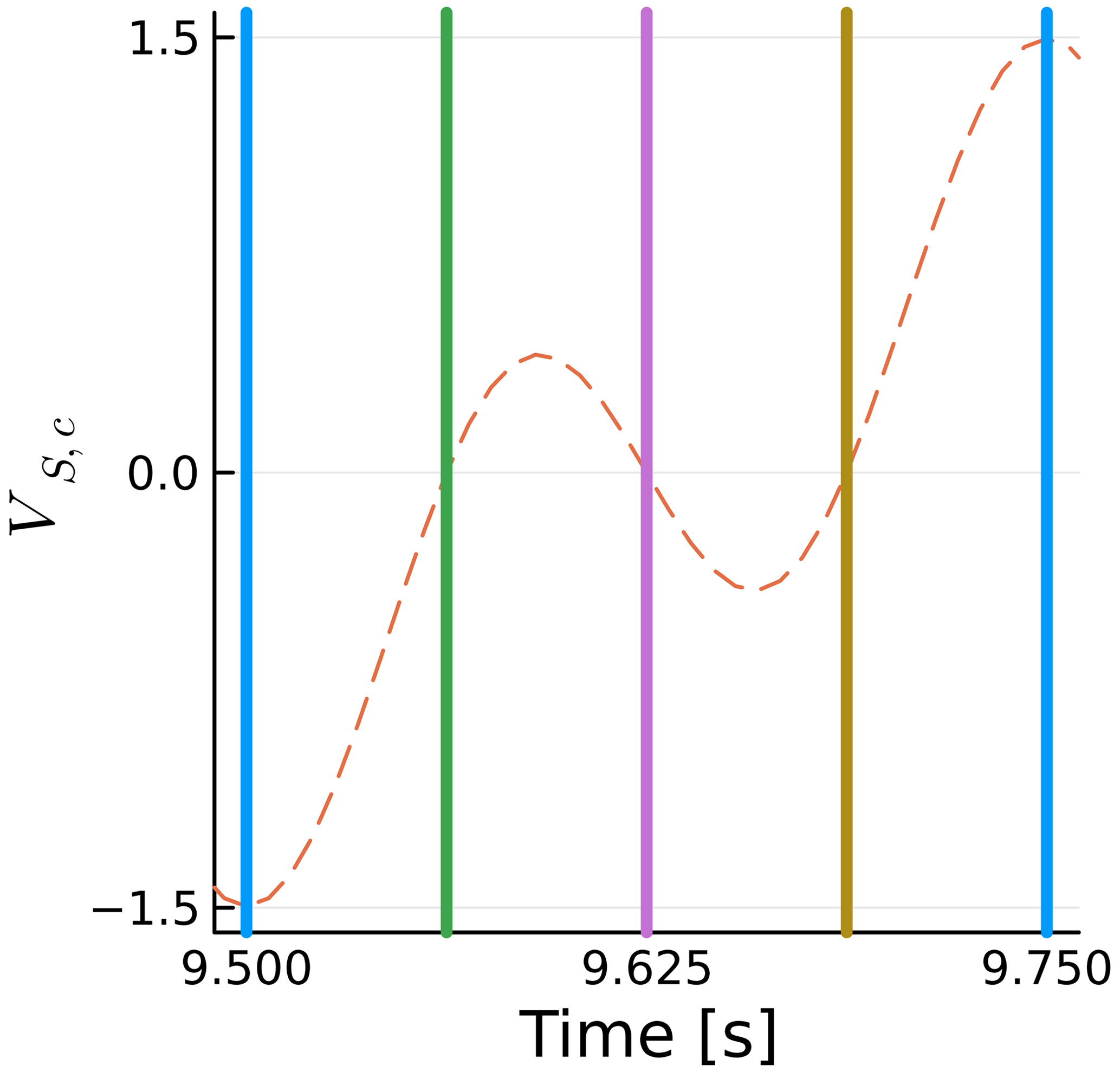
Figure 17 Time history of horizontal sway velocity projected on airfoil chord at the tip of blade 1. Vertical lines show blade azimuth.

Figure 18 Azimuth convention used. Blade shown at $\mathit{\psi }=\mathrm{270}{}^{\circ }$.

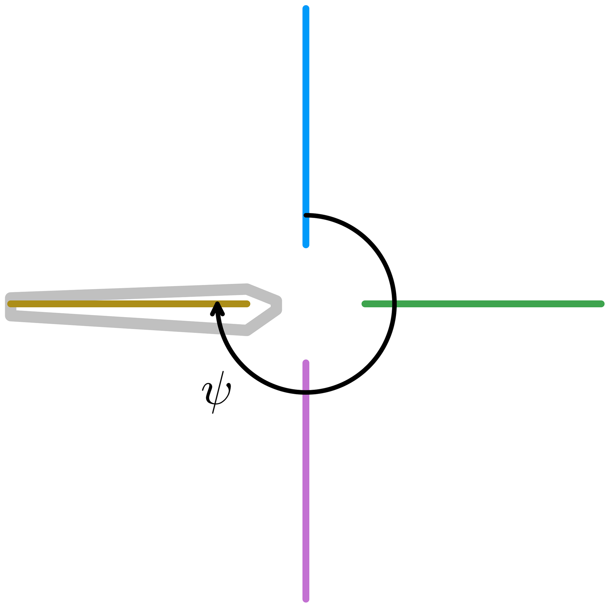
The horizontal rotor sway velocity varies with the cosine of the sway frequency f, while the projection onto the chord varies with the cosine of the rotational frequency f_Ω. When both functions are at their maxima with opposite signs, the maximum blade thrust is achieved, as seen at 9.75 s. When they are at their maxima with the same sign, the blade thrust is minimized, as seen at 9.5 s. The equation for the horizontal sway velocity projected onto the blade chord is

$$\begin{array}{}\text{(3)}& V_{\text{S,c}}=-\mathrm{2}\mathit{\pi }fA\cos \left(\mathrm{2}\mathit{\pi }ft\right)\cos \left(\mathrm{2}\mathit{\pi }{f}_{\mathrm{\Omega }}t\right).\end{array}$$

We can see that the thrust fluctuations in Fig. 16 are nearly directly proportional to V_S,c, as seen in Fig. 17, other than some differences that we will address in Sect. 4.4. All the other curves in Fig. 14 can be interpreted in similar ways. They are all at $\mathit{\psi }=\mathrm{0}{}^{\circ }$ at multiples of 0.25 s.

The general behavior for sway motion is as follows: when the blade is pointing to either side, the sway velocity projection onto the blade chord is zero, sway effects are minimal, and the thrust is near its mean value. When the blade is pointing up or down, the potential for sway effects is maximum and the thrust can reach its maximum or minimum if this coincides with maximum sway velocity. Hence, the relationship between the rotation and sway frequencies, along with the phase between the trigonometric functions that represent those motions, will dictate the behavior of the blade thrust.

4.3 Yawing turbine

We impose a yawing motion on the turbine by rotating it around the vertical central axis using the same conventions of Sect. 3. This results in a dynamic angle between the freestream velocity and the rotor axis, as in Fig. 11. The yaw amplitude is the maximum value of this angle, which we set to $A=\mathrm{3}{}^{\circ }$. Once again, the simulations are conducted with f varying between 1 and 5 Hz. The yawing motion introduces a velocity on the rotor relative to the rotation axis, which reaches its maximum at the tip radius R:

$$\begin{array}{}\text{(4)}& U_{\mathrm{Y}}=\mathrm{2}\mathit{\pi }fAR,\end{array}$$

where A must be in radians. As U_Y can act with or against U_∞, we do not adjust the flow velocity in the calculation of C_Tb.

Figure 19 shows the time history of C_Tb for different values of f. Results are remarkably similar to Fig. 14, with multiple frequencies involved and the pure sine response for f=4 Hz. Figure 20 shows ΔC_Tb as a function of $U_{\mathrm{Y}}/U_{\mathrm{\infty }}$ for the yaw cases. Results seem to indicate a linear trend throughout all cases, with some effects of blade choice and again a large decrease in thrust fluctuation when the yaw and rotation frequencies match, at $U_{\mathrm{Y}}/U_{\mathrm{\infty }}=\mathrm{0.4}$, as in sway. Surge cases are also included for reference as a function of U_S. This is the main reason for using U_Y in Fig. 20, as it allows us to compare surge and yaw in the same graph. If we used the reduced frequency, this would not account for the different motion amplitudes used in either case.

Figure 19 Time history of blade 1 thrust coefficient for various yaw frequencies.

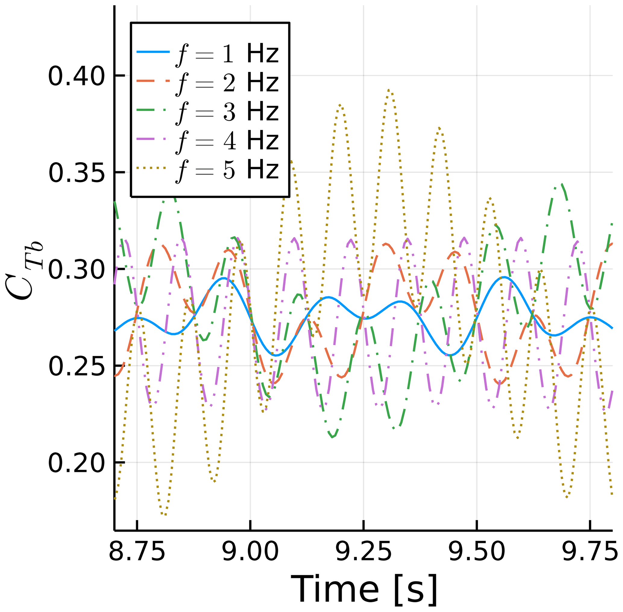
Figure 20 Amplitude of blade thrust coefficient fluctuations for various maximum surge velocities U_S and maximum tip yaw velocities U_Y.

Note that U_Y is not acting on the entire rotor plane. It acts mostly near the blade tips when they are horizontal. Hence, we see that, in spite of the more complex nonlinear behavior of the yaw motion, for comparable U_S and U_Y, the surging motion is more critical for blade loading. Taking into account phase cancellation effects of the three blades for yawing motion, the rotor forces (but not necessarily the rotor moments) acting on the tower will be less critical in yaw versus a comparable surge motion as well. Also noteworthy is that yaw seems to remain linear even at $U_{\mathrm{Y}}/U_{\mathrm{\infty }}=\mathrm{0.5}$, whereas the surge becomes nonlinear around $U_{\mathrm{S}}/U_{\mathrm{\infty }}=\mathrm{0.15}$.

Similar to the previous section, we now focus on a single yaw case, namely f=3 Hz, and zoom into the time history of C_Tb. This is shown in Fig. 21. The same conventions of Fig. 18 are used. Figure 22 shows the streamwise component of the blade tip yaw velocity U_Y,R. The force fluctuations are nearly proportional to −U_Y,R, as they are modulated by the yaw frequency f and rotational frequency f_Ω. Again, as in sway, the thrust fluctuation is nearly perfectly proportional to the velocity induced by the motion, although inversely proportional in this case. The blade tip velocity introduced by yaw as a function of time t is

$$\begin{array}{}\text{(5)}& U_{\text{Y,R}}=\mathrm{2}\mathit{\pi }fA\cos \left(\mathrm{2}\mathit{\pi }ft\right)R\sin \left(\mathrm{2}\mathit{\pi }{f}_{\mathrm{\Omega }}t\right),\end{array}$$

where the cosine corresponds to the velocity change due to yaw and the sine is due to the blade tip distance to the yaw axis changing with the blade azimuth. A negative U_Y,R is in the opposite direction as the freestream velocity, adding thrust.

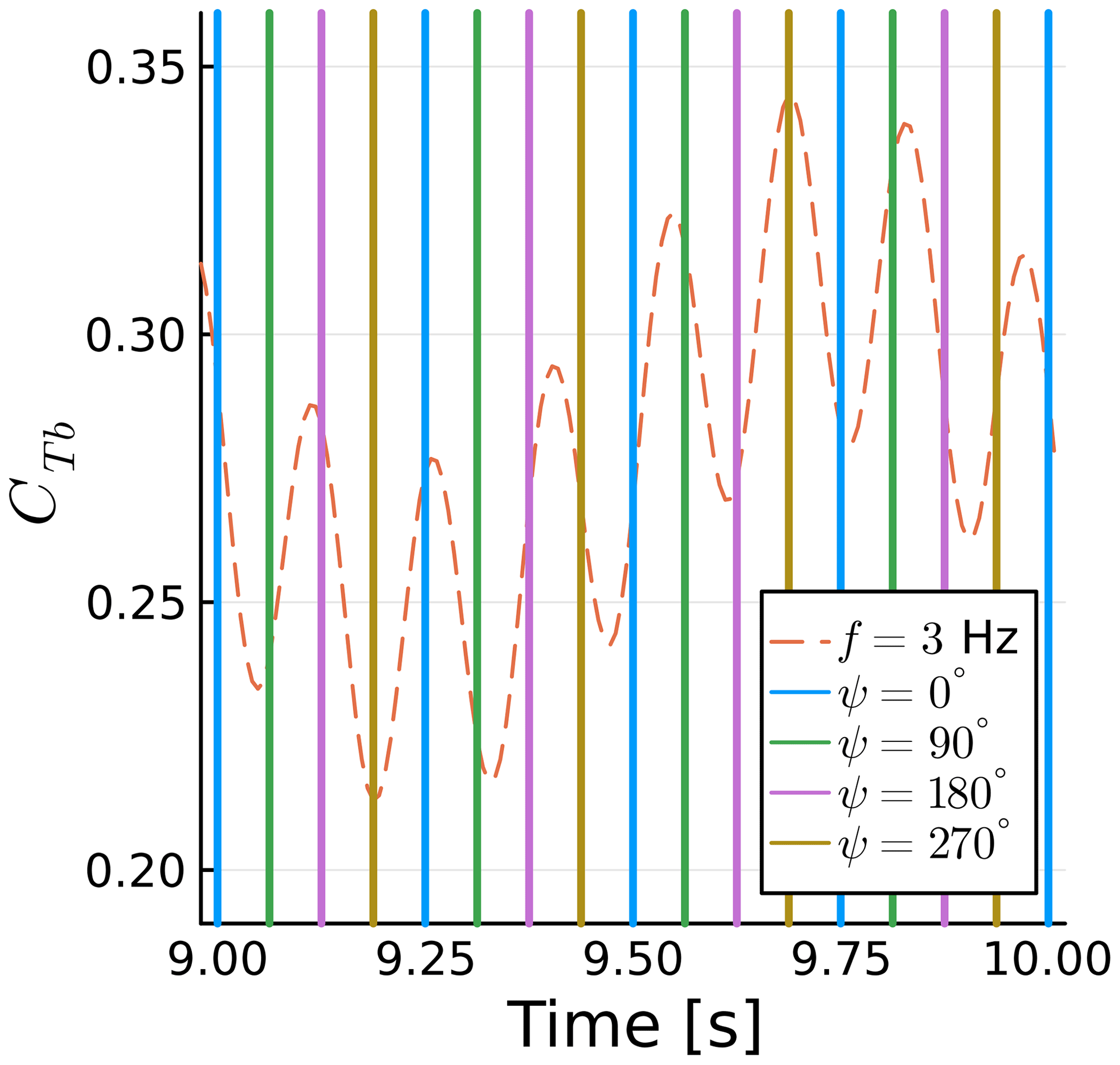
Figure 21 Time history of blade 1 thrust coefficient for a yaw case. Vertical lines show blade azimuth.

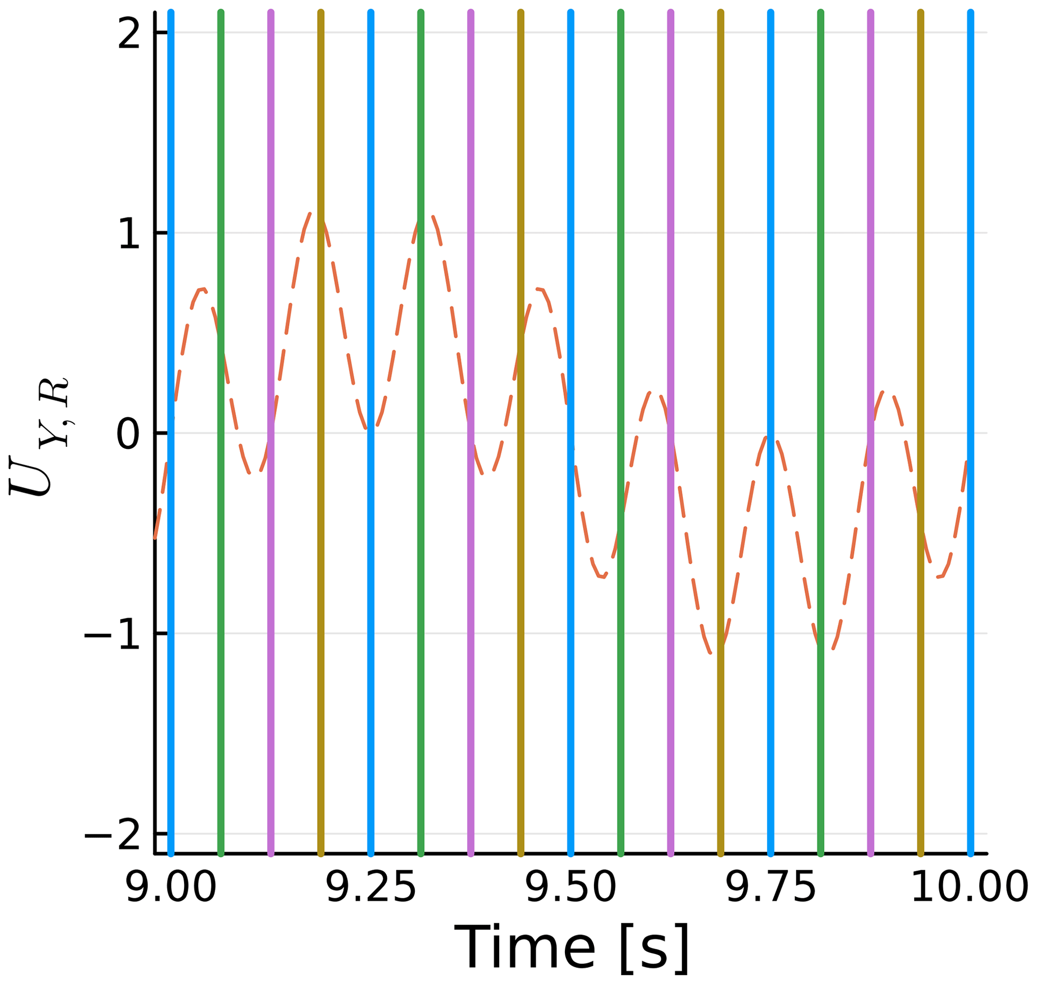
Figure 22 Time history of blade 1 streamwise blade tip yaw velocity. Vertical lines show blade azimuth.

The general behavior for yaw is as follows: when the blade is pointing up or down, the velocity introduced by the yaw force is zero and the thrust is near its mean value. This can be seen for all cases of $\mathit{\psi }=\mathrm{0}{}^{\circ }$ and $\mathit{\psi }=\mathrm{180}{}^{\circ }$. When the blade is at $\mathit{\psi }=\mathrm{90}{}^{\circ }$ or $\mathit{\psi }=\mathrm{270}{}^{\circ }$, there is a potential for high yaw effects if this coincides with high yaw velocities. This can be seen near 9.2 and 9.3 s. In other words, the amplitude of the thrust fluctuations is linked to the phase between the trigonometric functions describing the blade rotation and the yaw motion.

4.4 Effect of blade azimuth

The results shown so far for sway and yaw are all for single blades, which had a specific initial position, with blade 1 pointing up. The sway and yaw motions were all done with the rotor in neutral position at time equal to zero. The rotation frequency was 4 Hz, and the sway and yaw frequencies were 1, 2, 3, 4, and 5 Hz. Hence, the rotor motion and blade position were locked in phase, and this is not representative of all the possible loads blades can experience with different starting positions or with non-integer frequency ratios.

We can analyze Eqs. (3) and (5) to verify the amplitude of ΔC_Tb for arbitrary combinations of frequencies and phase. We can see that V_S,c is a function of the product of two cosines and U_Y,R a product of a sine and a cosine. Let us refer to these products as the phase-frequency amplitude, as they are linked to the phase of the trigonometric functions and the ratio of their frequencies. In both cases, the trigonometric products can vary in amplitude between 0.5 and 1, where 1 corresponds to the amplitude varying between −1 and 1. Hence, we can use the previous results, calculate the phase-frequency amplitude for each case, normalize the results by the phase-frequency amplitude, and then multiply them by 0.5 and 1. This will allow us to see the range of possible results for each sway and yaw amplitude for arbitrary combinations of frequencies and phase.

Figures 23 and 24 show the numerical results achieved for each blade in the previous simulations, along with the theoretical range of the results for arbitrary combinations of frequency ratios and starting blade position. The dashed lines represent the possible range of results based on each blade result with corresponding colors. For the yaw motion, in Fig. 24, we see that the range calculated based on each of the blades is always nearly identical. Hence, the thrust amplitude is behaving according to Eq. (5). The same can be said for most of the sway motion in Fig. 23; however, at ${\mathit{\beta }}_{\text{max}}=\mathrm{37}{}^{\circ }$, i.e., when the sway frequency is identical to the rotation frequency, all three curves are supposed to be at the bottom range of the prediction of Eq. (3), but in reality they are at different levels. Hence, there is a mismatch between the three ranges, showing that the sway results are not simply following Eq. (3), which is hinted at by the fact that the trends are nonlinear.

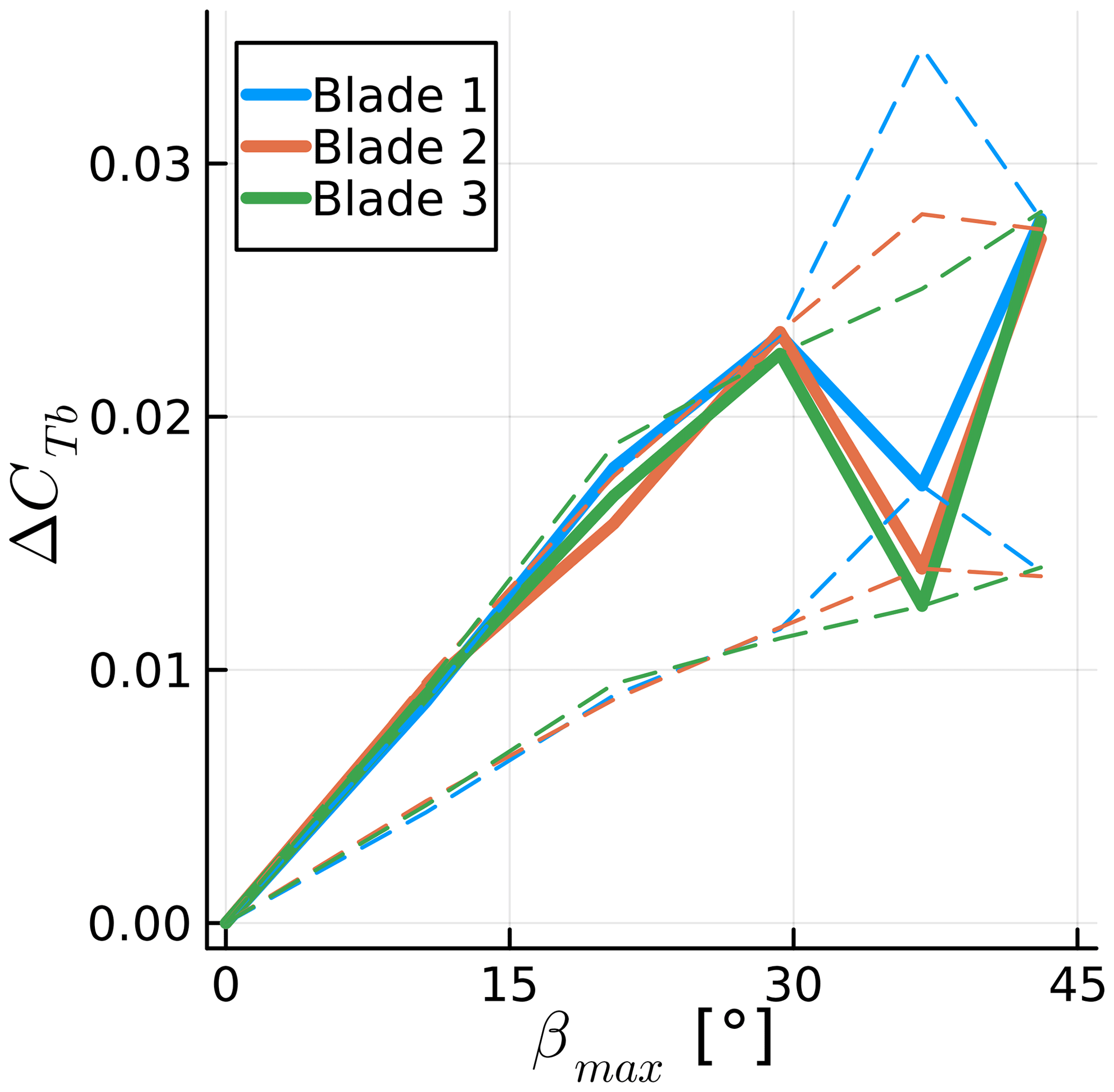
Figure 23 Amplitude of blade thrust coefficient fluctuation for various maximum side wind angles achieved during sway motion. Simulations results are shown, along with the theoretical possible range of results as dashed lines. Thrust normalized with maximum rotor velocity magnitude.

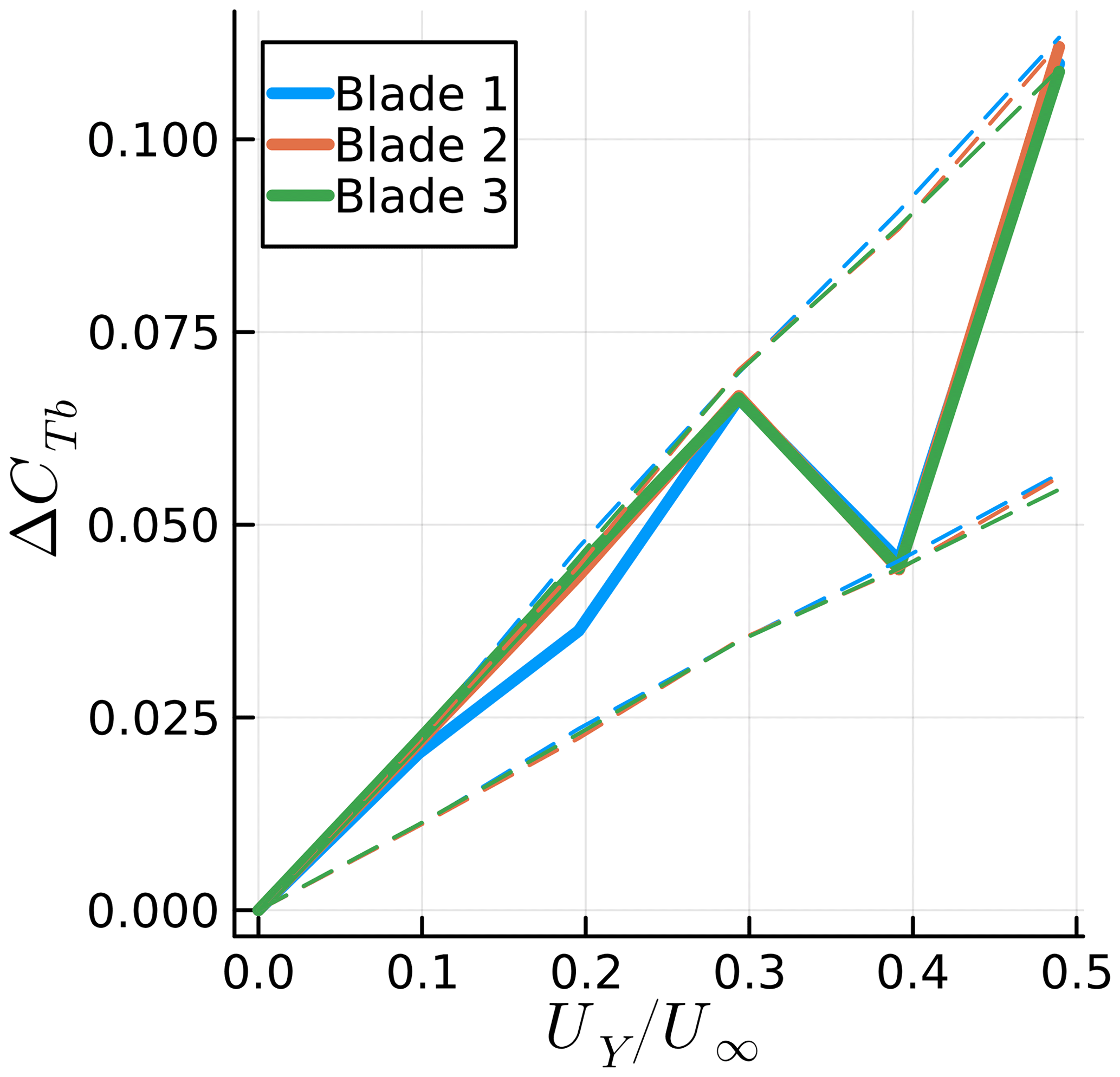
Figure 24 Amplitude of blade thrust coefficient fluctuation for various maximum tip yaw velocities. Simulations results are shown, along with the theoretical possible range of results as dashed lines.

The thrust fluctuations start by scaling linearly with the surge, sway, and yaw motions, as these motions act on the blade sections, increasing and decreasing the relative flow velocity. The surge and yaw motions act on the axial velocity of a given blade section, while the sway motion changes the tangential velocity on the blade sections. As the tangential velocity is typically much higher than the axial velocity in wind turbines, the sway motion effects are small compared to the surge and yaw. However, the sway motion moves the rotor out of the slipstream, leading to changes in axial velocity that are not due to simple changes in the kinematic velocities. This effect is quantified in the next section.

5 Wake motion sensitivity study

Methods such as BEM are unable to capture the detailed wake motion of wind turbines shown in Fig. 7, while the numerical dissipation of CFD also introduces challenges for preserving tip vortices. However, such methods are able to achieve accurate results for rotor motion (Mancini et al., 2020). Hence, we seek to quantify the impact of the wake induction on the blades for moving rotors. We achieve this by comparing the simulations in the previous sections with cases where the rotor is not surging, swaying, or yawing, but the effects of these motions are still present. Throughout this section we refer to these simulations as having pseudo motion.

To do this, we take advantage of the properties of panel methods and model the rotor motion indirectly. The rotation of the rotor is still performed explicitly, but the surge, sway, and yaw motion are included not by displacing the turbine but by modifying the equation for the sources σ and the unsteady Bernoulli equation, which computes the pressure p. In both equations, the panel kinematic velocity U_k is used. Hence, for the simulations with real motion in the previous sections, the rotors were displaced and their displacement was then included in σ and p as U_k. For the pseudo-motion simulations, we add the surge, sway, and yaw velocities to U_k for computing σ and p while not surging, swaying, and yawing the rotor.

The pseudo-motion method means that the wake panels are always released from the trailing edges in the fixed rotor position. The wakes are not identical to the wakes of a fixed rotating turbine, as changes in the circulation on the blades will affect how the wake is convected. However, the wakes are substantially different from the cases with real motion while still being more realistic than a frozen or prescribed wake method. With this, we seek to quantify the effect of real motion and the associated realistic wake compared to pseudo motion and the more simple wake that comes with it.

We select various frequencies from the previous sections and simulate them in pseudo motion. The results are summarized in Figs. 25 and 26. The mean thrust on the blades is predicted very well with pseudo motion, staying within 5 % of the real-motion results. The thrust fluctuation, however, varies substantially, in particular for sway cases. The sway case behaves differently from the others because as the rotor moves to the side, the undisturbed flow is allowed to energize the wake, moving it further away from the rotor in the axial direction. Concurrently, the rotor moving to the side means it is moving away from the wake induction in the lateral direction or moving outside of the stream tube and into the freestream flow. Thus a rotor in sway achieves lower axial induction and higher thrust, which is a counterintuitive combination. The variation in ΔC_Tb for sway in pseudo and real motion can also be explained by this interaction of the freestream flow and the wake. If we consider that on one side of the rotor the wake is stretched by the aforementioned interaction and on the other side the wake is compressed by the opposite effect, ΔC_Tb can be dampened or augmented by the real sway motion, depending on how the blade position is aligned with the lateral motion.

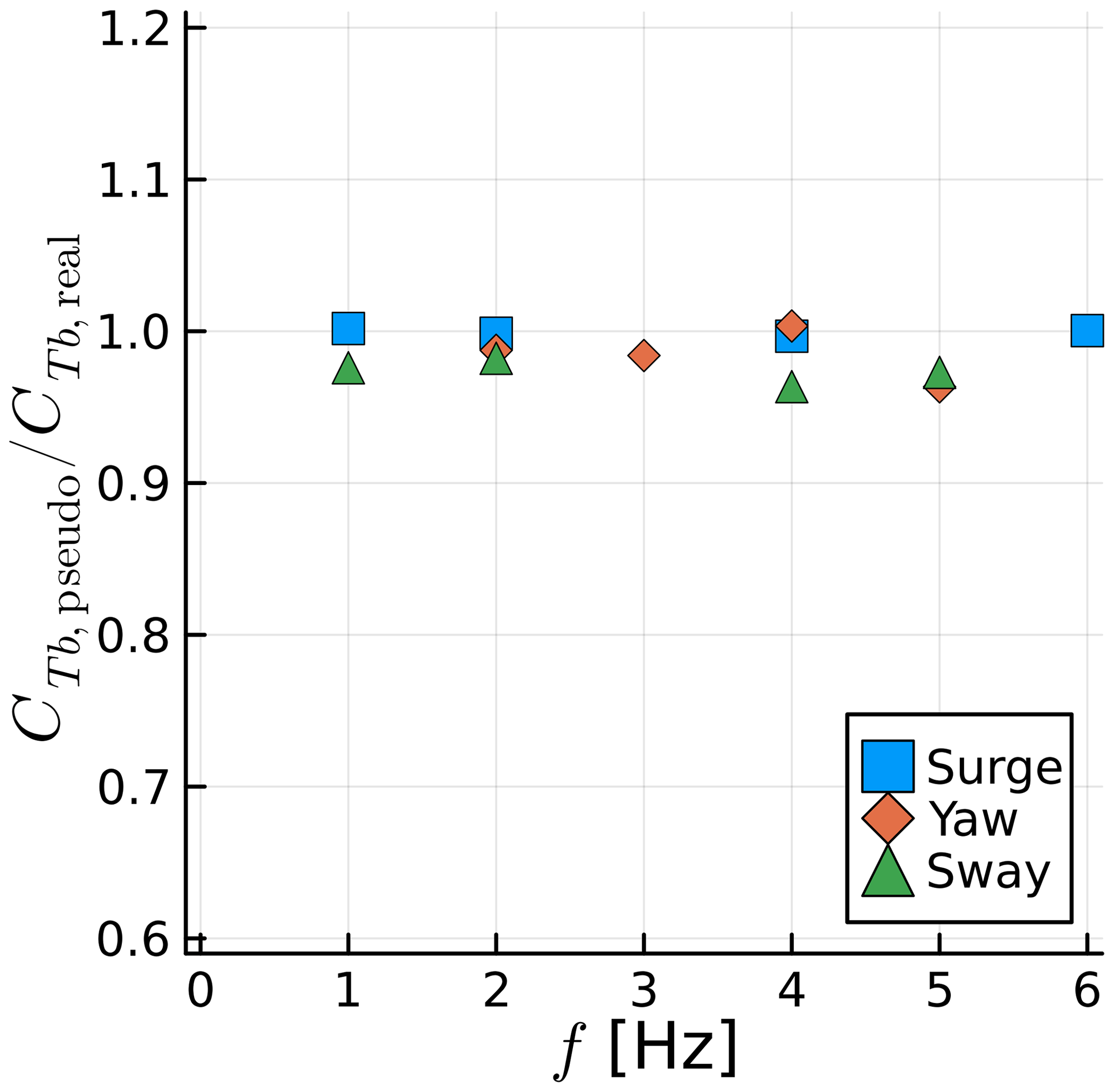
Figure 25 Ratio between mean blade thrust for pseudo-motion and real-motion simulations for various frequencies and motion types.

Figure 26 Ratio between amplitude of fluctuating blade thrust for pseudo-motion and real-motion simulations for various frequencies and motion types.

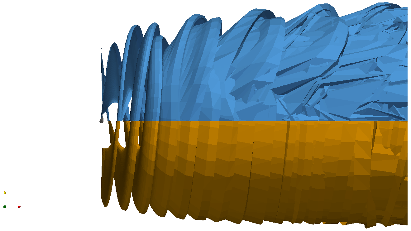
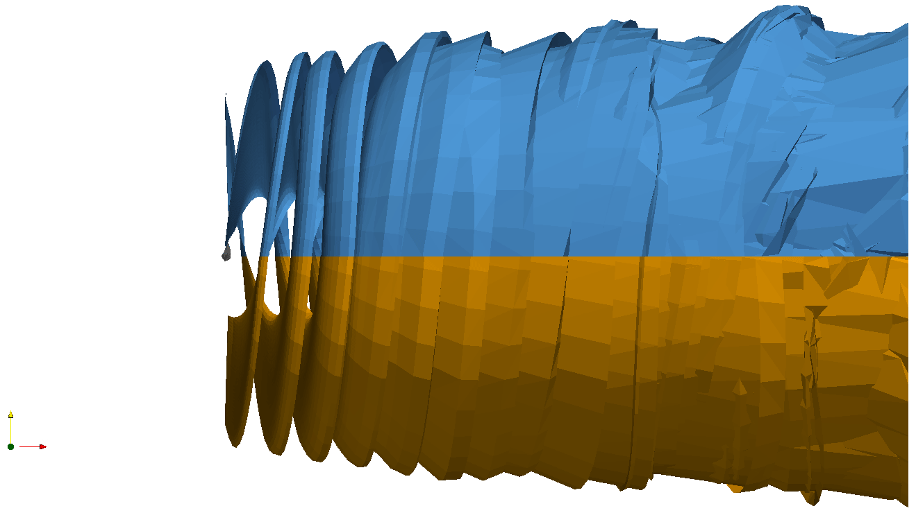
Figures 27–29 show the wakes for real and pseudo surge, sway, and yaw, respectively. The surge case uses axial symmetry; hence, only one blade is shown. The differences between real and pseudo motion in surge are subtle, while the yaw motion is more obvious, as the wake becomes more irregular in real motion due to the lack of symmetry. The sway case is quite extreme, with the pseudo motion showing a very well-behaved wake, almost identical to the other cases, while real motion makes the wake become chaotic very quickly.

Figure 27 Wake for real (top, blue) and pseudo (bottom, orange) surge motion at f=1 Hz. Only one blade shown.

Figure 28 Wake for real (top, blue) and pseudo (bottom, orange) sway motion at f=4 Hz.

Figure 29 Wake for real (top, blue) and pseudo (bottom, orange) yaw motion at f=3 Hz.

The amplitudes and frequencies used in this paper for surge are mostly related to the UNAFLOW experiment. For sway and yaw, we decided to use the same frequencies as in surge, adapting the amplitude to obtain values of ΔC_Tb of the same order of magnitude as the surge cases. While this is an arbitrary decision, we believe the results herein can be generalized. For surge, as long as the amplitude and frequencies do not lead to the wakes impinging on the blades, we have no reasons to believe the effect of wake motion will be severe. For sway, the amplitude chosen for this section is compatible with the turbine oscillating from side to side by less than 4^∘, which seems realistic for a FOWT. This is sufficient for the thrust fluctuations to be severely affected by wake motion, leading to the conclusion that sway motion is heavily affected by wake motion effects. Finally, for dynamic yaw motion with very high yaw amplitudes, a similar effect of wake motion as seen with sway could be encountered. However, we believe FOWT platforms do not tend to yaw dynamically at high amplitudes. Hence, we expect the wake motion effects for yaw to be small, in general.

6 Conclusions

We have shown that a free-wake panel method can accurately capture the mean and unsteady thrust of a surging wind turbine. The methodology used in this paper slightly underpredicts the mean thrust and overpredicts the amplitude of thrust fluctuations; however, results are comparable to and in line with the state-of-the-art (Mancini et al., 2020).

The effects of the rotor motion on the tip vortices was also shown to be accurately captured by the method in what we believe is the first simulation of surging wind turbine wakes that accurately reproduce experimental data. Wake vortices are particularly difficult to capture with CFD methods, as the Eulerian approach tends to dissipate them (Bayati et al., 2018a). Lagrangian methods have a significant advantage in preserving the wake vortices near the body, with the disadvantage of wake entanglement far from the rotor, which in turn requires some dissipation for stabilization.

We found that the surge frequency had to be tripled from its maximum value in the experimental campaign to reach a nonlinear response in thrust. The current method allowed us to investigate this by isolating Theodorsen effects. This means that, in reality, the nonlinear response could happen earlier due to other phenomena, such as dynamic stall.

We then studied side wind, sway motion, and yaw motion of a rotor. We demonstrated the complexity of the forces acting on the blades during sway and yaw motions even without flow separations. By comparing side wind results with sway results using the maximum sway angle and including the sway velocity in the thrust coefficient, we were able to show linear behavior for sway at low frequencies that matched the side wind trends. For the yaw motion, the blade tip surge effect was demonstrated by investigating the axial force on a single blade during a yaw cycle. For both sway and yaw, the blade force fluctuations can vary by a factor of 2, depending on the ratio between the rotor motion and rotation, as well as the blade initial position.

Finally, we used an interesting feature of the current methodology to perform what we refer to as pseudo-motion simulations, where we accounted for the surge, sway, and yaw motion on the rotor without actually performing these motions on the turbine. With this we showed the sensitivity of wake deformation on the forces on the blades. It was found that the sway motion allows undisturbed air to enter the wake, increasing the mean thrust and, in our case, reducing the dynamic loads. Surge and yaw were shown to be fairly insensitive to the wake motion, which explains the fact that methods that do not capture wake dynamics can still predict surge motion effects well.

This work is a stepping stone towards building a tool that is able to simulate FOWTs in a way that is accurate, robust, and efficient. Future work will expand to include more complex cases, such as full offshore platform motion and aeroelasticity.

Appendix A: Nomenclature

BEM	Blade element momentum theory
CFD	Computational fluid dynamics
FOWT	Floating offshore wind turbine
A	Surge, sway, or yaw motion amplitude
Aij	Doublets influence coefficient matrix
Ar	Reduced amplitude ($A/D$)
Bij	Sources influence coefficient matrix
Ciw	Wake vortices influence coefficient matrix
CT	Rotor thrust coefficient
D	Wind turbine rotor diameter
f	Surge, sway, or yaw motion frequency
fr	Reduced surge frequency ($fD/U_{\mathrm{\infty }}$)
fΩ	Rotor rotation frequency
p	Pressure
R	Wind turbine rotor radius
T	Rotor thrust
t	Time
U	Surface flow velocity
Uk	Panel kinematic velocity
US	Rotor maximum surge velocity (2πfA)
UY	Maximum yaw tip velocity 2πfAR
U∞	Freestream velocity
VS	Maximum sway velocity (2πfA)
VS,c	Sway velocity projected onto blade chord
x	Instantaneous rotor streamwise position
$\dot{x}$	Instantaneous rotor surge velocity
β	Side wind angle
βmax	Maximum side wind angle due to sway motion
	(${\tan }^{-\mathrm{1}}(V_{\mathrm{S}}/U_{\mathrm{\infty }})$)
γ	Wake vortex strength
ΔCT	Rotor thrust coefficient fluctuation amplitude
ΔCTb	Blade thrust coefficient fluctuation amplitude
Δψ	Rotor rotation angle in one time step
μ	Doublet strength
ρ	Air density
σ	Source strength
Φ	Velocity potential
ϕ	Phase between rotor surge motion and thrust
ψ	Blade azimuth angle