The wind farm as a sensor: learning and explaining orographic and plant-induced flow heterogeneities from operational data

This paper describes a method to identify the heterogenous flow characteristics that develop within a wind farm in its interaction with the atmospheric boundary layer. The whole farm is used as a distributed sensor, which gauges through its wind turbines the flow field developing within its boundaries. The proposed method is based on augmenting an engineering wake model with an unknown correction field, which results in a hybrid (grey-box) model. Operational SCADA (supervisory control and data acquisition) data are then used to simultaneously learn the parameters that describe the correction field and to tune the ones of the engineering wake model. The resulting monolithic maximum likelihood estimation is in general ill-conditioned because of the collinearity and low observability of the redundant parameters. This problem is solved by a singular value decomposition, which discards parameter combinations that are not identifiable given the informational content of the dataset and solves only for the identifiable ones.

The farm-as-a-sensor approach is demonstrated on two wind plants with very different characteristics: a relatively small onshore farm at a site with moderate terrain complexity and a large offshore one in close proximity to the coastline. In both cases, the data-driven correction and tuning of the grey-box model results in much improved prediction capabilities. The identified flow fields reveal the presence of significant terrain-induced effects in the onshore case and of large direction and ambient-condition-dependent intra-plant effects in the offshore one. Analysis of the coordinate transformation and mode shapes generated by the singular value decomposition help explain relevant characteristics of the solution, as well as couplings among modeling parameters. Computational fluid dynamics (CFD) simulations are used for confirming the plausibility of the identified flow fields.

1 Introduction

Understanding and modeling wind farm flows is one of the key grand challenges facing wind energy science (Veers et al., 2019). The problem is extremely complex because wind farm flows are driven by a number of interconnected physical phenomena, which are not only difficult to model but also in part still poorly understood.

Within this very wide field, the present work tries to explore the idea of using the whole wind plant as a distributed sensor that, interacting with the atmospheric boundary layer, responds to it and, consequently, effectively measures the flow developing within its own boundaries. Exploiting this idea, can data from a wind plant be used to detect significant features in the flow, in support of an improved understanding of key driving phenomena? Can the same data be leveraged to derive more accurate flow models? Finally, how can the knowledge already encapsulated in existing models be combined with the information contained in the data?

These questions are explored here in relation to engineering wake models.

1.1 Engineering wake models and their limitations

Within the plethora of wind farm flow models that have been developed, engineering wake models have carved an extremely successful niche for themselves at the lower end of the fidelity spectrum. In fact, they now support a wide range of use cases, from wind plant design to wind farm flow control (Meyers et al., 2022). Engineering wake model suites, like for example FLORIS (FLOw Redirection and Induction in Steady State) (NREL, 2021) and PyWake (Pedersen et al., 2019), are based on the bottom-up concept of superimposing relatively simple flow elements, such as wake deficit, wake-added turbulence, wake deflection, and wake combination. The success of engineering wake models is due to their modularity, which allows for a rapid uptake of any new improvement to the individual submodels, but also due to their speed, which is key in supporting repetitive tasks such as design, control, uncertainty quantification, and others.

However, like all models, engineering wake models are not an exact copy of reality and are unable to precisely match field measurements. For example, the comprehensive survey of Lee and Fields (2021) showed that, although modeling techniques have greatly improved in recent years, inaccuracies in the estimation of the turbine inflow speed are still the largest contributor to the uncertainty in yield assessments.

A first reason for the mismatch between predictions and reality is the unsuitable calibration of the model parameters. For example, wake recovery is affected by atmospheric conditions and terrain roughness (Abkar et al., 2016; Wu and Porté-Agel, 2012), which depend on location and on time (for example, because of seasonal vegetation changes). Therefore, default standard values of the parameters describing recovery might not be appropriate for a specific site nor for a specific time at that site.

Additionally, engineering wake models approximate (but do not exactly resolve) only some (but not all) physical processes that take place in and around a wind plant.

For example, the influence of terrain orography is difficult to capture for onshore wind farms, and high-fidelity models may be necessary to adequately resolve all flow effects (for example, see Berg et al., 2011, for the Bolund site and Palma et al., 2020, for the Perdigão site). Neglecting terrain effects can indeed increase the uncertainty of predictions generated by engineering models (Fleming et al., 2019; Doekemeijer et al., 2021). FLORIS, which is the software framework used in this work, currently does not include a terrain flow model but offers the possibility of interpolating a set of wind speeds provided at different locations, for example obtained from met masts (Farrell et al., 2021). However, even with the inclusion of this heterogeneous background flow, the model still assumes wakes to follow the ground contour and neglects the fact that terrain features may induce pressure gradients, local deviations of wake trajectories, changes in dissipation rate, flow separations, and other effects (Porté-Agel et al., 2020; Politis et al., 2012; Castellani et al., 2017). Terrain and ground roughness can also affect offshore sites. For example, a Doppler radar deployed at the Westermost Rough wind farm (Nygaard and Newcombe, 2018) and computational fluid dynamics (CFD) simulations at Anholt (van der Laan et al., 2017) revealed the development of heterogeneous flow fields caused by the influence of the neighboring coastlines.

The interaction of a wind farm with the atmospheric boundary layer (ABL) is another extremely complex process, which has not yet always been properly accounted for in engineering models. In general, several flow regions can be distinguished around and within a wind farm (Porté-Agel et al., 2020). Upstream, the induction zone is a region of decreasing flow speed, causing a phenomenon termed “blockage” (Wu and Porté-Agel, 2017; Segalini and Dahlberg, 2020), which has been observed through production data (Bleeg et al., 2018) and by long-range lidar measurements (Schneemann et al., 2021). Efforts at modeling this effect include the aggregation of individual turbine induction zone models (Nygaard et al., 2020; Branlard et al., 2020) and the use of the linearized Navier–Stokes equations (Segalini, 2021). Moving further downstream, an internal boundary layer starts growing over the turbines. If the farm is deep enough in the streamwise direction, the flow may reach a fully developed state, sometimes referred to as the “deep-array” condition (Calaf et al., 2010). In the fully developed region, momentum is only replenished by the vertical transport from the free atmosphere flowing above the farm. Theoretical models for an asymptotic flow regime have been developed under the assumption of an infinitely large wind farm (Frandsen et al., 2006). However, it is not clear at which distance from the leading edge a fully developed flow regime is reached (Wu and Porté-Agel, 2017); additionally, models typically assume a regular wind farm layout, a condition that is rarely met in practice. The flow has complex features not only within the wind plant but also at its perimeter. In fact, the flow has been reported to accelerate as it turns around the edges of a wind farm (Mitraszewski et al., 2013). Furthermore, CFD studies suggest that wind farms – similarly to hills, mountains, and other large orographic features – could generate gravity waves, which might not only affect the flow high above the turbines but also cause a redistribution of the available wind resource within the plant (Allaerts and Meyers, 2018). All of these phenomena appear to be strongly dependent on the ABL height and on atmospheric stability, with stable conditions typically amplifying their effects (Wu and Porté-Agel, 2017; Schneemann et al., 2021).

Yet another poorly understood and modeled effect is the way wakes interact, mix, and merge together. Current models range from simple superposition laws, e.g., the sum of squares freestream superposition (SOSFS) method (Katic et al., 1986) or the freestream linear superposition (FLS) one (Lissaman, 1979); to more sophisticated physics-based combination models (Zong and Porté-Agel, 2020; Bastankhah et al., 2021); and to methods that describe how wakes merge with the background flow (Lanzilao and Meyers, 2022). Despite these advances, new modeling proposals will take time for validation and adoption, while the simple SOSFS and FLS superposition laws are still heavily relied on. In conditions where many wake interactions take place, such models can have a substantial influence on the results (Hamilton et al., 2020).

1.2 Improvement to engineering models by data-driven tuning and learning

There are three main approaches to deal with the deficiencies of current engineering wake models.

The first is to eliminate the resolved part of the model altogether and use a black box to learn the complete system behavior from data. Indeed, data-driven machine learning methods are a growing trend in many fields, including fluid mechanics (Brunton et al., 2020). Wind energy applications are no exception to this trend: for example, Göçmen and Giebel (2018) and Bleeg (2020) have proposed black-box farm flow models based on neural networks. While this approach seems appealing at first sight, it also neglects the large body of knowledge and experience already encapsulated in existing models. Additionally, trying to distill new understanding and physical insight from black boxes is in general not a trivial task. More importantly, one should never forget that the data informational content always caps what a purely date-driven model can deliver: what is not in the data, can never be learned. As a consequence, large amounts of data are typically necessary to derive useful models.

The second approach is to improve a (white) model by tuning its parameters. For example, van Beek et al. (2021) tuned the parameters of the FLORIS model using operational data, which resulted in a substantial error reduction. However, tuning the resolved physics in a model when relevant unresolved phenomena are present may lead to nonphysical results. In this sense, one should be wary of approaches that only tune the parameters of an existing model, unless one can guarantee that there are no relevant missing physical effects in that model. As previously argued, this is typically not the case with present engineering wake models.

The third possible approach is to directly acknowledge the hybrid nature of the problem. This means augmenting the resolved model with parametric corrections that represent the unmodeled physics, resulting in the so-called grey-box approach. Data are used to tune the parameters of the resolved model and to learn the ones of the corrections. These two processes of tuning and learning are clearly intimately linked, and should be conducted simultaneously. In the framework of wind farm flows, the approach of simultaneous tuning and learning (STL) was first proposed by Schreiber et al. (2020a). The concept was demonstrated by augmenting the FLORIS wake model (NREL, 2021; Fleming et al., 2020) with various “surgical” ad hoc corrections, designed to represent non-uniform inflow, secondary steering, and other unmodeled effects. The method has since been applied also to a wind tunnel study (Campagnolo et al., 2022) and to a joint flow model comparison (Göçmen et al., 2022). The resulting – possibly highly redundant – parameter estimation problem was solved using a maximum likelihood approach based on the singular value decomposition (SVD). The role of this decomposition is to map the original correlated and redundant physical parameters into uncorrelated ones. This simplifies the understanding of which parameters can be identified based on the informational content of the data and which are undiscernible. Once the visible parameters are identified, they are transformed back into the physical ones through the inverse map.

In the present paper, the STL approach is extended by augmenting a wake model with a heterogeneous background flow, which can be considered a correction to the normally assumed uniform ambient flow. In this way, the whole wind plant becomes a distributed sensor that “feels” the flow that develops within its boundaries; this has suggested the name of “farm as a sensor” to this approach. The similar concept of the “the turbine as a sensor” has been developed by the senior author and his collaborators, where a wind turbine is turned into a sensor that “feels” the inflow at its rotor disk; interested readers can refer to Kim et al. (2023), Bertelè et al. (2017), Schreiber et al. (2020b), and Bertelè et al. (2021) and references therein.

The paper is organized as follows. Section 2 describes the wind farm flow model (Sect. 2.1), its parameterization (Sect. 2.2), and the identification technique used to tune and learn the free model parameters from operational data (Sect. 2.3). Section 3 describes the application to an onshore wind farm at a site of moderate complexity (Sect. 3.1) and to a large offshore plant (Sect. 3.2). Finally, Sect. 4 reports the main findings of this work and provides an outlook towards further future developments.

2 Methods

2.1 Wind farm flow

2.1.1 Temporal decomposition

Within a wind plant, the scalar wind speed field U at some reference height can be decomposed in the time domain as

$$\begin{array}{}\text{(1)}& U=\overline{U}+\stackrel{\mathrm{̃}}{U}+U^{\prime }.\end{array}$$

The term $\overline{U}$ represents a constant-in-time component. The term $\stackrel{\mathrm{̃}}{U}$ accounts for the slow temporal variability caused by changes in ambient conditions and in the turbine set points, as well as their advection downstream throughout the plant. Finally, the term U^′ accounts for fast fluctuations caused by turbulence.

Engineering models such as FLORIS (NREL, 2021) provide only for a steady-state (as opposed to time-resolved) representation of a turbulent wake immersed in a turbulent flow. Nonetheless, it is important to realize that the long-term effects of U^′ are indeed included in such models. In fact, the wake geometry in the model is represented by an “average” path and shape, observed over a long-enough period of time. In this way, the wake model implicitly includes the effects of meandering caused by turbulent fluctuations in the wind field. Additionally, the model accounts for the effects of both the local ambient and wake-added turbulence intensity (TI), denoted $I=\mathrm{SD}\left(U^{\prime }\right)/\overline{U}$, which affects the behavior (and especially the recovery) of the wake. The inclusion of these effects in the model also helps clarify the split between the slow scales $\stackrel{\mathrm{̃}}{U}$ and the fast scales U^′ and provides guidelines on where in the frequency spectrum one ends and the other one begins. In fact, a wake model is calibrated by fitting it to observations that have been averaged over a certain window of time (typically, equal to 10 min). Consequently, $\stackrel{\mathrm{̃}}{U}$ represents all the slower timescales that have not already been taken into account by this time averaging. Such scales are neglected in a steady-state model and explicitly considered in a dynamic one (e.g., see the FLORIDyn dynamic wake model; Gebraad and van Wingerden, 2014).

This work considers the steady-state behavior of wind plants for given ambient and operating conditions. Consequently, the wind field model includes only the component $\overline{U}$ (which, as just argued, implicitly includes the effects of the turbulent component U^′), whereas $\stackrel{\mathrm{̃}}{U}$ is neglected. For notation simplicity, in the following the bar notation is dropped and the steady state wind field is simply denoted U.

2.1.2 Causal decomposition

The wind speed field can be causally decomposed as

$$\begin{array}{}\text{(2)}& U=U_{\mathrm{amb}}+\mathrm{\Delta }{U}_{\mathrm{wake}}+\mathrm{\Delta }{U}_{\mathrm{amb}\leftrightarrow \mathrm{wake}}.\end{array}$$

The first term U_amb represents the undisturbed ambient flow at the site, in the absence of the wind turbines and their induced effects. This component of the flow depends on the state of the ABL and on the surface conditions, the latter including the effects of local orography (onshore) and of local roughness (caused by vegetation and small-scale terrain features in the onshore case and by sea state in the offshore one). This distinction of surface causal effects can also be seen as a further scale decomposition, the largest spatial scales being attributed to orography and the smallest ones to roughness.

The second term ΔU_wake represents the change in speed caused by wakes, as modeled by FLORIS or similar models. This flow component depends on the state of the ABL, on the local ambient conditions at each turbine (including the possible presence of wakes released by upstream machines), and on the turbine characteristics and their operating set points.

The third and last term ΔU_amb↔wake represents the interaction between the undisturbed ambient flow and the one generated by the turbines, and it can be further decomposed as

$$\begin{array}{}\text{(3)}& \mathrm{\Delta }{U}_{\mathrm{amb}\leftrightarrow \mathrm{wake}}=\mathrm{\Delta }{U}_{\mathrm{amb}\to \mathrm{wake}}+\mathrm{\Delta }{U}_{\mathrm{wake}\to \mathrm{amb}}.\end{array}$$

The term ΔU_amb→wake accounts for the effects of the ambient background flow on the wake. It should be noted that several of these effects are already included by design in engineering wake models: for example, ambient turbulence intensity (Bastankhah and Porté-Agel, 2014), vertical shear, and veer (Sezer-Uzol and Uzol, 2013) are known to affect the wake characteristics, and their modeling approximations are included in FLORIS (NREL, 2021). Hence, all of these effects, as well as possible future refinements designed to better reflect the influence of the characteristics of the ABL on wake behavior, already appear in the term ΔU_wake. Therefore, the term ΔU_amb→wake is tasked here with representing only the modifications to the wake trajectory and shape caused by the heterogeneity of the ambient flow (Bossanyi, 2018) and by terrain orography and roughness changes (Politis et al., 2012). These phenomena affect the behavior of wakes not only parallel to the terrain but also in the vertical direction. Indeed, wind tunnel (Hyvärinen et al., 2018) and large-eddy simulation (LES) (Wise et al., 2022; Shamsoddin and Porté-Agel, 2018) studies show that wakes only partially follow the terrain contour, as they tend to separate from it on the leeward side of a hilltop (Shamsoddin and Porté-Agel, 2018) and in unstable atmospheric conditions (Wise et al., 2022). In the present study, these complex effects are neglected, and wakes simply follow the ground contour. Consequently, the term ΔU_amb→wake is dropped from the discussion. However, when models for these effects finally become available, their presence will not alter the rest of the present formulation.

The term ΔU_wake→amb represents the effects caused by the plant, i.e., the turbines and their wakes, on the ambient undisturbed flow. These include both intra-plant (array) effects (which, for example, cause the average flow to slow down within the plant (Calaf et al., 2010) and to locally accelerate in between turbines (McTavish et al., 2015)) and extra-plant effects (which cause the growth of a boundary layer over the plant and result in blockage (Porté-Agel et al., 2020) and local edge effects (Mitraszewski et al., 2012)).

In summary, the causal decomposition of the flow speed expressed by Eq. (2) can be re-written as

$$\begin{array}{}\text{(4)}& U=U_{\mathrm{0}}+\mathrm{\Delta }{U}_{\mathrm{wake}}+\mathrm{\Delta }U.\end{array}$$

The first term U₀ is the average uniform (i.e., spatially constant) wind speed. The second term ΔU_wake represents the wake deficit model, as implemented in FLORIS or similar tools. The third term is a heterogeneous correction that is written as

$$\begin{array}{}\text{(5)}& \mathrm{\Delta }U=\mathrm{\Delta }{U}_{\mathrm{amb}}+\mathrm{\Delta }{U}_{\mathrm{wake}\to \mathrm{amb}},\end{array}$$

where ΔU_amb accounts for ambient surface-induced effects and ΔU_wake→amb for the effects of the turbines and wakes on the ambient flow. In this paper, both of these causes are aggregated into one single correction term ΔU. Disentangling these two effects should in principle be possible by using suitable datasets, as only the latter depends on the turbine operating conditions.

A similar causal decomposition is assumed for wind direction Γ and for turbulence intensity I. In fact, for both of these flow characteristics similar arguments apply, as both can exhibit a heterogeneous behavior induced by surface effects and by the interaction of the flow with the turbines and their wakes. Hence, noting a generic field as F (where F=U, F=Γ, or F=I), the assumed causal model is written as

$$\begin{array}{}\text{(6)}& F=F_{\mathrm{0}}+\mathrm{\Delta }{F}_{\mathrm{wake}}+\mathrm{\Delta }F.\end{array}$$

For given ambient and operating conditions, F₀ is a site-average (i.e., spatially constant) flow condition (either speed, direction, or turbulence intensity). ΔF_wake is the wake model; at present, in addition to the speed deficit, FLORIS includes secondary steering for F=Γ and wake-added TI for F=I. Finally, ΔF is a heterogeneous (spatially variable) correction field. When considering the wind direction field, i.e., F=Γ, the correction needs to be applied in a circular manner with modulus 360^∘.

The functional dependency of the heterogeneous correction term ΔF is assumed to be in the form

$$\begin{array}{}\text{(7)}& \mathrm{\Delta }F=\mathrm{\Delta }F\left({\mathit{A}}_{\mathrm{0}},Q\right),\end{array}$$

where $\mathit{A}=(U,\mathrm{\Gamma },I,L{)}^T$ is a vector of ambient state variables, L is the Obukhov length, subscript (⋅)₀ indicates an average (spatially constant) quantity, and Q represents a spatial location. Hence, the correction term ΔF depends on the following.

• The site-average ambient conditions (A₀). In fact, different wind speeds, directions, turbulence intensities, and stability characteristics induce different interactions of the ambient flow with the surface and the plant.

• The spatial position (Q). Surface conditions (including both orographic and roughness effects) and plant-induced phenomena are typically heterogeneous.

• The turbine set points. However, it should be noted that this dependency is already implicitly taken into account by the dependency of ΔF on A₀ and Q because turbine set points depend on local ambient conditions. An extra parameter could be used to account for different operating modes (for example, a quiet mode for nighttime operation), but it is neglected for simplicity here and also because it is not used in the application examples.

2.2 Model parameterization

It is the primary goal of this paper to present a method for computing a best estimate of the flow fields expressed by Eq. (6), based on operational data. For given ambient conditions F₀, this requires first expressing the terms ΔF and ΔF_wake in terms of free parameters (which is discussed in Sect. 2.2.1 and 2.2.2, respectively) and then estimating the values of such parameters based on an optimality criterion, using available field measurements (which is explained in Sect. 2.3). In principle, the identification should ensure the satisfaction of fluid conservation properties for the resulting field expressed by Eq. (6); such constraints are, however, neglected in the present implementation. Once the values of the parameters have been computed, the resulting identified model can be used for performing new predictions in support of various use cases.

2.2.1 Heterogeneous flow parameterization

The spatial heterogeneity of field ΔF over the farm area is discretized using a 2D mesh, where the value of the field at a generic point Q is obtained by interpolating discrete nodal values p_F through assumed shape functions n(Q). Notice that this implies that the site is assumed to be flat, consistently with the current FLORIS model; as a result, the speedup, for example, caused by a hill is represented as a patch of increased velocity. The 2D spatial interpolation is expanded in additional 1D dimensions to capture the influence of the environmental conditions A₀. For example, when considering the effects of ambient wind direction variability (Γ₀), the range of wind directions is discretized into a desired number of nodal direction values, and assumed 1D shape functions are used to interpolate such values. This results in a different set of spatial speed nodes for each wind directional node, creating a 3D interpolation of flow speed accounting for spatial position and wind direction. This dependency of the interpolating functions on space and ambient conditions is expressed in symbols as n(A₀,Q). Terrain and plant-induced effects can generate different heterogeneities in the speed, direction, and turbulence intensity fields. Hence, different meshes with different resolutions and node locations can in principle be used for each one of the three fields.

The parameterization of the ΔF field can be written as

$$\begin{array}{}\text{(8)}& \mathrm{\Delta }F\left({\mathit{A}}_{\mathrm{0}},Q\right)={\mathit{n}}^T\left({\mathit{A}}_{\mathrm{0}},Q\right)p_{\mathrm{F}}.\end{array}$$

The spatial dependency of ΔF is implemented in FLORIS through the heterogeneous flow functionality introduced in Farrell et al. (2021).

Alternatively, the heterogeneous field ΔF can also be defined as

$$\begin{array}{}\text{(9)}& \mathrm{\Delta }F\left({\mathit{A}}_{\mathrm{0}},Q\right)=\mathrm{\Delta }{F}_{\mathrm{NP}}\left({\mathit{A}}_{\mathrm{0}},Q\right)+{\mathit{n}}^{\mathrm{T}}\left({\mathit{A}}_{\mathrm{0}},Q\right)p_{\mathrm{F}}.\end{array}$$

Here, the first term is a non-parametric (i.e., which will not be identified) heterogenous flow field. This term could be obtained from on-site measurements (Farrell et al., 2021) or, as shown later on in Sect. 3.1.6, from over-the-terrain CFD simulations. When this term is used, the parametric term n^T(A₀,Q)p_F, instead of being charged with the modeling of the complete heterogeneity of the flow, has the role of modeling only differences between the non-parametric flow field and the actual one. The inclusion of the non-parametric term might have two beneficial effects on the identification: first, it reduces the magnitude of the heterogeneity that has to be learned from data, and, second, it provides a non-uniform initial guess for the identification algorithm, possibly easing its convergence.

2.2.2 Wake model parameterization

The ΔF_wake component of the flow is computed through the FLORIS engineering wake model (NREL, 2021). The velocity deficit ΔU_wake is modeled with the kinematic Gaussian model by Bastankhah and Porté-Agel (2014). Wakes are combined with the SOSFS method (Katic et al., 1986) in Sect. 3.1 and with FLS (Lissaman, 1979) and SOSFS in Sect. 3.2. Wake-added turbulence ΔI_wake is considered through the Crespo and Hernandez (1996) turbulence model.

In general, FLORIS and similar models are characterized by the following functional dependency:

$$\begin{array}{}\text{(10)}& \mathrm{\Delta }{F}_{\mathrm{wake}}=\mathrm{\Delta }{F}_{\mathrm{wake}}\left({\mathit{A}}_{\mathrm{0}},Q,\mathit{k}\right),\end{array}$$

where k represents a vector of model-specific parameters (NREL, 2021). Following Schreiber et al. (2020a), the model-specific parameters are not tuned directly; rather, the baseline value (denoted k_init) of one parameter is added to an unknown calibration term (denoted p_k), i.e.,

$$\begin{array}{}\text{(11)}& k=k_{\mathrm{init}}+p_k.\end{array}$$

All calibration parameters p_k are collected in the vector of the to-be-tuned parameters p_W. Examples of the parameters and their changes caused by calibration are given later on (see Table 2 in Sect. 3.1.3 and Table 5 in Sect. 3.2.5).

Notice that, in addition to the “native” parameters of the FLORIS model, additional extra parameters can be used to augment the model with ad hoc correction terms. Schreiber et al. (2020a) used this technique to target specific deficiencies in the model. For example, the baseline wake model was augmented with a local wind direction term to account for secondary steering, which was not natively implemented at the time in FLORIS. Similarly, Campagnolo et al. (2022) introduced a correction to the power loss model for yawed conditions.

2.3 SVD-supported identification

Stacking the parameters for the heterogeneous flow correction and the parameters for wake model tuning, the final vector of the to-be-identified parameters is

$$\begin{array}{}\text{(12)}& \mathit{p}=\left[\begin{array}{c}{\mathit{p}}_U\\ {\mathit{p}}_{\mathrm{\Gamma }}\\ {\mathit{p}}_I\\ {\mathit{p}}_W\end{array}\right].\end{array}$$

Notice that one single parameter vector is defined, comprising both the parameters that define the unknown heterogenous flow and the ones that tune the wake model. This means that the learning of the heterogeneous flow is performed simultaneously to wake model tuning. In fact, if one were to estimate the two components ΔF and ΔF_wake one after the other, any error committed in the estimation of the first would affect the second, and the results would be sequence dependent. Since this cannot be, given that both terms eventually contribute to the fields F, the two terms need to be estimated simultaneously.

Following a classical approach (Jategaonkar, 2006), a likelihood function is used to express the probability that a given set of noisy observations can be explained by a specific set of parameters. The parameter identification problem is then cast as the maximization of this likelihood function. This problem, however, is very likely ill posed. First, it is uncertain if all parameters are really observable given the existing measurements. Additionally, the parameters might not all be independent of each other, resulting in similar effects on the solution.

This dilemma is overcome by performing the identification through a singular value decomposition (SVD). The SVD-supported identification approach is general and can be applied to various problems: for example, Bottasso et al. (2014) used it for identifying airfoil polars and Schreiber et al. (2020a) for learning unrepresented effects in a wind farm flow model. The main idea behind this method is to map the original physical parameters into uncorrelated ones, using a linear rotational transformation of the problem unknowns computed through the SVD. Examination of the new set of parameters reveals the ones that are identifiable – because they have an acceptably low variance – and the ones that are not – because their variance is excessively large. Only the former parameters are retained in the process, and, once they have been identified, they are mapped back through the inverse transformation, recovering a solution in terms of the original physical parameters. Since many practical identification problems are nonlinear, this linear transformation of the unknowns is applied iteratively until convergence. This method has the advantage of working well even in the presence of unobservable or collinear parameters simply because only the visible ones are retained in the process. Additionally, an inspection of the transformation that maps the original into the uncorrelated parameters reveals useful insight into the interdependencies among parameters; an example of such an analysis is given later on in Sect. 3.1.4. For a complete derivation of the method, the reader is referred to Schreiber et al. (2020a), whereas here only a synthetic description is provided.

A steady wind farm flow model can be written as the following nonlinear functional expression:

$$\begin{array}{}\text{(13)}& \mathit{y}=\mathbf{f}(\mathit{p},\mathit{A}),\end{array}$$

where y indicates a vector of model outputs for which corresponding measurements z are available. In the present work, these quantities are represented by the power outputs of N_t wind turbines in a wind plant; however, the definition of the outputs is clearly problem dependent, so other measurements – when available – could be readily used. The inevitable discrepancy between measurements z and model outputs y is captured by the residual, which is defined as

$$\begin{array}{}\text{(14)}& \mathit{r}=\mathit{z}-\mathit{y}.\end{array}$$

Given a set of N observations $\mathit{\{}{\mathit{z}}_{\mathrm{1}},{\mathit{z}}_{\mathrm{2}},\mathrm{\dots },{\mathit{z}}_N\mathit{\}}$, the likelihood function (Jategaonkar, 2006) is

$$\begin{array}{}\text{(15)}& J\left(\mathit{p}\right)={\left((\mathrm{2}\mathit{\pi }{)}^{N_{\mathrm{t}}}\det \left({\mathbf{R}}^{-\mathrm{1}}\right)\right)}^{-N/\mathrm{2}}\exp \left({\displaystyle \frac{\mathrm{1}}{\mathrm{2}}}\sum _{i=\mathrm{1}}^N{\mathit{r}}_i^{\mathrm{T}}\mathbf{R}{\mathit{r}}_i\right),\end{array}$$

where R is the measurement noise covariance matrix. The maximum likelihood estimate (MLE) of the parameters is obtained by minimizing the negative logarithm of Eq. (15), i.e.,

$$\begin{array}{}\text{(16)}& {\mathit{p}}_{\mathrm{MLE}}=\arg {\min }_{\mathit{p}}-\ln J\left(\mathit{p}\right).\end{array}$$

The observability of the parameters can be gauged by the inverse of the Fisher information matrix $\mathbf{E}\in {\mathbb{R}}^{N_{\mathrm{p}}\times N_{\mathrm{p}}}$, which is defined as (Jategaonkar, 2006)

$$\begin{array}{}\text{(17)}& {\mathbf{E}}^{-\mathrm{1}}={\left[\sum _{i=\mathrm{1}}^N{w}_i{\left[{\displaystyle \frac{\partial {\mathit{y}}_i}{\partial \mathit{p}}}\right]}^{\mathrm{T}}{\mathbf{R}}^{-\mathrm{1}}\left[{\displaystyle \frac{\partial {\mathit{y}}_i}{\partial \mathit{p}}}\right]\right]}^{-\mathrm{1}}=\mathbf{P}.\end{array}$$

Factors w_i express an optional relative weight $w_i/\sum _{j=\mathrm{1}}^N{w}_j$ that can be attributed to an observation to boost its presence in the dataset, for example because it occurs multiple times (Karampatziakis and Langford, 2010).

An important result of MLE theory is that the ith diagonal element of P provides a lower bound (called Cramér–Rao bound) on the variance of the corresponding estimated parameter, while correlations among different parameters are captured by the off-diagonal terms (Jategaonkar, 2006). This highlights what is indeed the main problem of a naive formulation of the identification problem cast in terms of the original physical parameters p: even if a parameter has a high variance, typically it cannot be eliminated because of its (in general) non-negligible couplings to other parameters. This problem is solved when the SVD is used to diagonalize the inverse Fisher matrix P by a linear transformation of the unknowns. Since the transformed parameters are now uncorrelated, parameters that have a high variance – i.e., that are not visible given the available set of measurements – can be readily eliminated. The diagonalization of the inverse Fisher matrix is obtained by first factorizing it as E=M^TM, where factor $\mathbf{M}\in {\mathbb{R}}^{N_{\mathrm{t}}N\times N_{\mathrm{p}}}$ is

$$\begin{array}{}\text{(18)}& \mathbf{M}=\left[\begin{array}{c}\sqrt{w_{\mathrm{1}}}{\mathbf{R}}^{-\mathrm{1}/\mathrm{2}}\frac{\partial {\mathit{y}}_{\mathrm{1}}}{\partial \mathit{p}}\\ \sqrt{w_{\mathrm{2}}}{\mathbf{R}}^{-\mathrm{1}/\mathrm{2}}\frac{\partial {\mathit{y}}_{\mathrm{2}}}{\partial \mathit{p}}\\ \mathrm{⋮}\\ \sqrt{w_N}{\mathbf{R}}^{-\mathrm{1}/\mathrm{2}}\frac{\partial {\mathit{y}}_N}{\partial \mathit{p}}\end{array}\right].\end{array}$$

This matrix can now be decomposed by the SVD (Wall et al., 2003) through numerically efficient algorithms (Harris et al., 2020) in the product:

$$\begin{array}{}\text{(19)}& \mathbf{M}=\mathbf{U}\mathbf{\Sigma }{\mathbf{V}}^{\mathrm{T}},\end{array}$$

where the columns of $\mathbf{U}\in {\mathbb{R}}^{N_{\mathrm{t}}N\times N_{\mathrm{t}}N}$ and $\mathbf{V}\in {\mathbb{R}}^{N_{\mathrm{p}}\times N_{\mathrm{p}}}$ are, respectively, the left and right singular vectors of M. The matrix of left singular vectors U expresses the relative importance of the individual observations, while the matrix of right singular vectors V carries information on the correlation of the parameters. Matrix $\mathbf{\Sigma }=[\mathbf{S},\mathbf{0}{]}^{\mathrm{T}}$ contains the singular values s_i, which are sorted in descending order in the diagonal matrix $\mathbf{S}\in {\mathbb{R}}^{N_{\mathrm{t}}\times N_{\mathrm{t}}}$. By combining Eq. (19) and the factorization of E, the eigendecomposition of the inverse Fisher matrix can now be written as

$$\begin{array}{}\text{(20)}& \mathbf{P}={\mathbf{VS}}^{-\mathrm{2}}{\mathbf{V}}^{\mathrm{T}},\end{array}$$

i.e., the columns of V are the eigenvectors of P, whereas the entries of S⁻² are its eigenvalues. This suggests a transformation of the original parameters p, which are rotated through matrix V to yield a new set of parameters θ, i.e.,

$$\begin{array}{}\text{(21)}& \mathit{\theta }={\mathbf{V}}^{\mathrm{T}}\mathit{p}.\end{array}$$

Crucially, the covariance of the new parameters is now S⁻², which by definition is a diagonal matrix. Consequently, the new parameters are statistically decoupled. Their respective variance $s_i^{-\mathrm{2}}$ is readily obtained by the corresponding element in S. The Cramér–Rao bound (Jategaonkar, 2006) on the variance of the MLE estimates of the transformed parameters θ_MLE is

$$\begin{array}{}\text{(22)}& {\mathbf{S}}^{-\mathrm{2}}\le \mathrm{Var}\left({\mathit{\theta }}_{\mathrm{MLE}}-{\mathit{\theta }}_{\mathrm{true}}\right),\end{array}$$

where θ_true are the true (but clearly unknown) parameters. Therefore, a small singular value s_i corresponds to a large uncertainty in the estimate of the corresponding transformed parameter.

This important result is used to set an observability threshold ${\mathit{\sigma }}_{\mathrm{t}}^{\mathrm{2}}$, which defines the highest acceptable variance: every parameter with a variance above the threshold is deemed unobservable. This condition is enforced by retaining in the identification a transformed parameters i only if it satisfies the condition

$$\begin{array}{}\text{(23)}& s_i^{-\mathrm{2}}\le {\mathit{\sigma }}_{\mathrm{t}}^{\mathrm{2}}.\end{array}$$

This leads to a partitioning of the parameter vector θ into identifiable (denoted with the subscript ID) and non-identifiable (denoted with the subscript NID) sets, i.e.,  $\mathit{\theta }=[{\mathit{\theta }}_{\mathrm{ID}}^{\mathrm{T}},{\mathit{\theta }}_{\mathrm{NID}}^{\mathrm{T}}{]}^{\mathrm{T}}$, which induces a corresponding partitioning of the transformation matrix $\mathbf{V}=[{\mathbf{V}}_{\mathrm{ID}},{\mathbf{V}}_{\mathrm{NID}}]$ (and, clearly, also of U). The MLE identification is then performed for the sole identifiable parameters θ_ID. At the end of the convergence process, the orthogonal parameters are mapped back to the physical ones using

$$\begin{array}{}\text{(24)}& \mathit{p}\approx {\mathbf{V}}_{\mathrm{ID}}{\mathit{\theta }}_{\mathrm{ID}}.\end{array}$$

Choosing a lower threshold implies that fewer parameters are deemed trustworthy and are retained in the solution; this might reduce the quality of the solution if meaningful terms are discarded, but it will also reduce the computational cost and will typically ease convergence. On the other hand, picking a higher threshold has the opposite effect.

For guiding the solution, it is useful to enforce bounds on the parameters in the form ${\mathit{p}}_{\mathrm{lb}}\le \mathit{p}\le {\mathit{p}}_{\mathrm{ub}}$. Additionally, to improve conditioning, it is advisable to scale each parameter p_i with its respective bounds as

$$\begin{array}{}\text{(25)}& {\widehat{p}}_i={\displaystyle \frac{p_i-\left(p_{i_{\mathrm{ub}}}+p_{i_{\mathrm{lb}}}\right)/\mathrm{2}}{\left(p_{i_{\mathrm{ub}}}-p_{i_{\mathrm{lb}}}\right)/\mathrm{2}}},\end{array}$$

so that $-\mathrm{1}\le {\widehat{p}}_i\le \mathrm{1}$.

3 Results

The result section is divided in two parts, each examining a specific site. The Sedini and Anholt wind farms represent a typical mid-size onshore and large offshore case, respectively. These two plants are characterized by different wind climates and dominating flow effects, whose very distinct features are useful for assessing the generality of the proposed STL method. Furthermore, the quality and quantity of SCADA (supervisory control and data acquisition) data typically differ from site to site on account of different turbine types, acquisition systems, sampling frequencies, failure rates, miscalibration of sensors, and several other effects; here again, the use of different plants can help verify the robustness of a method that operates based on operational data of such variable quality and quantity. An overview of some key characteristics of the two wind plants is provided in Table 1, while Fig. 1 shows their layouts side by side, illustrating their typical spacings and overall size.

Table 1 Comparison of the main characteristics of the Sedini and Anholt wind farms.

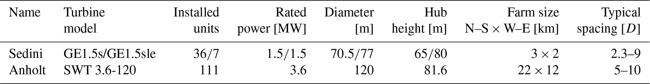
Figure 1 Layout and flow correction grid for the Sedini (a) and Anholt (b) wind farms. The symbol D_S stands for the rotor diameter at Sedini and D_A for the diameter at Anholt, whose respective values are given in Table 1. The two figures are at the same scale in terms of diameters, i.e., 1 D_S on the left panel has the same length as 1 D_A on the right one. At the same kilometer scale, the Sedini farm looks much smaller than the Anholt one because D_A≫D_S.

The Sedini wind farm is located in the north of Sardinia, a large island off the western coast of Italy. A subgroup of turbines was the subject of a wind farm flow control test campaign, using both wake steering and axial induction control. Because of this previous activity, the behavior of the farm had been already examined with different wake models (Bossanyi and Ruisi, 2021; Doekemeijer et al., 2021). At this site, the terrain is complex, both outside and within the boundaries of the wind plant, vegetation is present, and the turbines are of two different types and heights, all characteristics that make the Sedini wind plant a challenging onshore test case. The farm is designed for minimum wake losses in the prevalent (westerly) wind direction, and significant wake effects are only expected for specific turbines. In addition to the layout, Fig. 1a shows also the grid of flow correction nodes, which was based, for simplicity, on a regular mesh. Node spacing was adjusted to capture the most relevant terrain effects.

The Anholt offshore wind farm is located about 20 km east of the Danish coast in the Kattegat, a shallow sea between the Jutland peninsula and the west cost of Sweden. The presence of the Jutland coastline influences the western inflow to the farm, creating a gradient that was already investigated by van der Laan et al. (2017), Peña et al. (2018), and Doekemeijer et al. (2022). Given the absence of the small-scale orographic effects present at Sedini, a coarser grid of flow correction nodes was chosen in this case. On the other hand, this large array with numerous wake interactions is an interesting test case for the presence of significant intra- and extra-plant effects (Nygaard, 2014).

3.1 The Sedini wind farm

3.1.1 Site overview, dataset analysis, and preprocessing

Figure 2 shows a more detailed layout of the plant, including the turbine identifiers and a colormap of the terrain elevation. The behavior of the plant is investigated for the main, western wind sector between 245 and 310^∘. From these directions, the farm is only two rows deep, and the heterogeneous correction of Eq. (5) is expected to be dominated by the term ΔF_amb. The goal of the present test case is therefore to show the ability of the proposed method of learning the orography-induced inhomogeneities of the intra-plant flow purely from the available SCADA data.

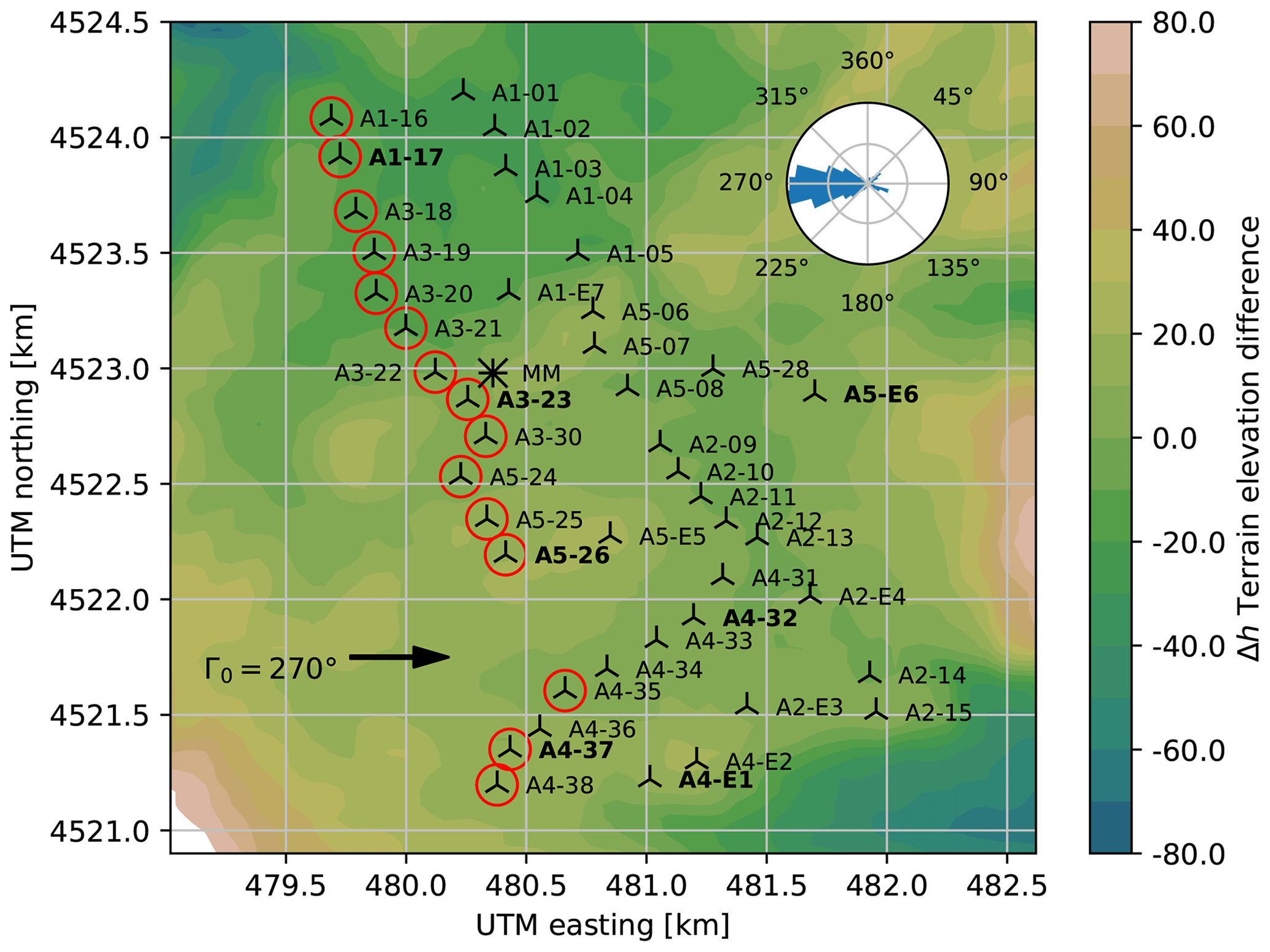
Figure 2 Layout of the Sedini wind farm. The colormap shows the height difference with respect to the average terrain elevation. A bold identifier indicates turbines used to determine the average wind direction Γ₀. For an exemplary wind direction of 270^∘, free-stream turbines are marked with a red circle. The wind rose shows the frequency of Γ₀ over the period of time analyzed in the present study. The met mast is indicated by the symbol ∗.

For this study, SCADA data at 10 min sampling frequency were made available for the years 2015 and 2016, whereas meteorological mast measurements were made available for the years 2008–2010. Since the two time periods do not overlap, the mast data were used only to analyze the general climate at the site (Kern et al., 2017).

The data were first cleaned of entries where turbines were not reporting to the acquisition system. Next, for every timestamp, the average wind direction Γ₀ was determined from the yaw readings of selected “sensing” turbines. This required a careful correction of the readings, since yaw sensors were observed to be significantly affected by biases and drifts. These effects were mitigated by exploiting wake interactions among turbines. In fact, biases were eliminated by looking at the minima of the power ratio between neighboring waked/waking turbines as functions of wind direction and comparing them with the interactional directions expected from the farm layout. Drifts were eliminated by observing the shift over time of these minima and removing them from the time series. Notwithstanding these corrections, since the yaw readings of some turbines appeared to be quite unreliable, only a cluster of eight machines was finally used to determine the wind direction.

Because short-term fluctuations $\stackrel{\mathrm{̃}}{F}$ are neglected in this work, data preprocessing was performed to obtain binned observations dominated by the steady component F, according to the methods described by Schreiber et al. (2018). To omit short-term propagation effects, a stationary filter was applied to the data streams. Similarly to Hansen et al. (2012), a data point was discarded if the wind direction change exceeded ±2.5^∘ compared to the previous 10 min value. The wind speed measured by the nacelle anemometers exhibited significant discrepancies among neighboring turbines, indicating possible miscalibrations. This problem was solved by computing a rotor equivalent wind speed (REWS) from the power curve, following the approach already used by Schreiber et al. (2018) on the same dataset; this is clearly only possible between cut-in and rated wind speed (i.e., between 4 and 13 m s⁻¹ for the GE1.5s). The ambient wind speed U₀=〈U_FS〉 was determined by averaging the REWS of turbines operating in free stream. The determination of whether a turbine is in free stream or not was based on the prediction of the plant flow model by first guessing the wind speed and then iterating. The seven turbines of type GE1.5sle (whose identifiers in Fig. 2 contain the letter “E”) were not used for determining the wind speed; since they are characterized by a taller hub height than the other ones, this would have required the use of the vertical shear, introducing further uncertainties.

Additional ambient conditions such as TI, shear, and density – although certainly significant for wake behavior and turbine performance and loading – cannot be typically derived in a straightforward manner exclusively from the turbine SCADA data. Göçmen and Giebel (2016) and Mittelmeier et al. (2017) proposed methods to deduce TI and density from SCADA data, but unfortunately the necessary channels were not available in the present case. This problem was solved by the inspection of the met-mast recordings, which suggested that TI and shear are strongly dominated by the diurnal cycle at this site. Based on this indication, the dataset was split in daytime and nighttime regimes, based on the local time of sunset and sunrise (Beauducel, 2022). The diurnal characteristic values were derived from historical met-mast readings. For daytime conditions the shear was set to α₀=0.09 and the TI to I₀=0.15, whereas for the nighttime case the values α₀=0.18 and I₀=0.125 were used. An analysis of the met-mast data revealed also that, for the westerly 245–310^∘ sector of interest for this study, TI and shear exhibit only a very modest variability with wind direction; this, on other hand, is in general not the case when considering the whole wind rose because of the different direction-dependent land and sea fetches. Density was set to the constant average value ρ₀=1.177 kg m⁻³. After filtering, the remaining 2102 timestamps were grouped and averaged in day and night bins of width equal to 5^∘ for wind direction and 2 ms⁻¹ for wind speed, resulting in N=36 observations. Half of the bins were picked randomly to form the training dataset, whilst the other half were reserved for testing.

3.1.2 STL parameter identification

The output vector y (see Eq. 13) was defined as the normalized generated power of every turbine, i.e.,

$$\begin{array}{}\text{(26)}& \mathit{y}={\displaystyle \frac{\mathrm{1}}{P_{\mathrm{ref}}}}\left[\begin{array}{c}{P}_{\mathrm{WT}\mathrm{1}}\\ \mathrm{⋮}\\ P_{\mathrm{WT}\mathrm{43}}\end{array}\right],\end{array}$$

where P_ref=1.5 MW is the rated power of the GE turbines. Power was calculated in 1^∘ wide direction steps, eventually averaging the results over each 5^∘ bin sector.

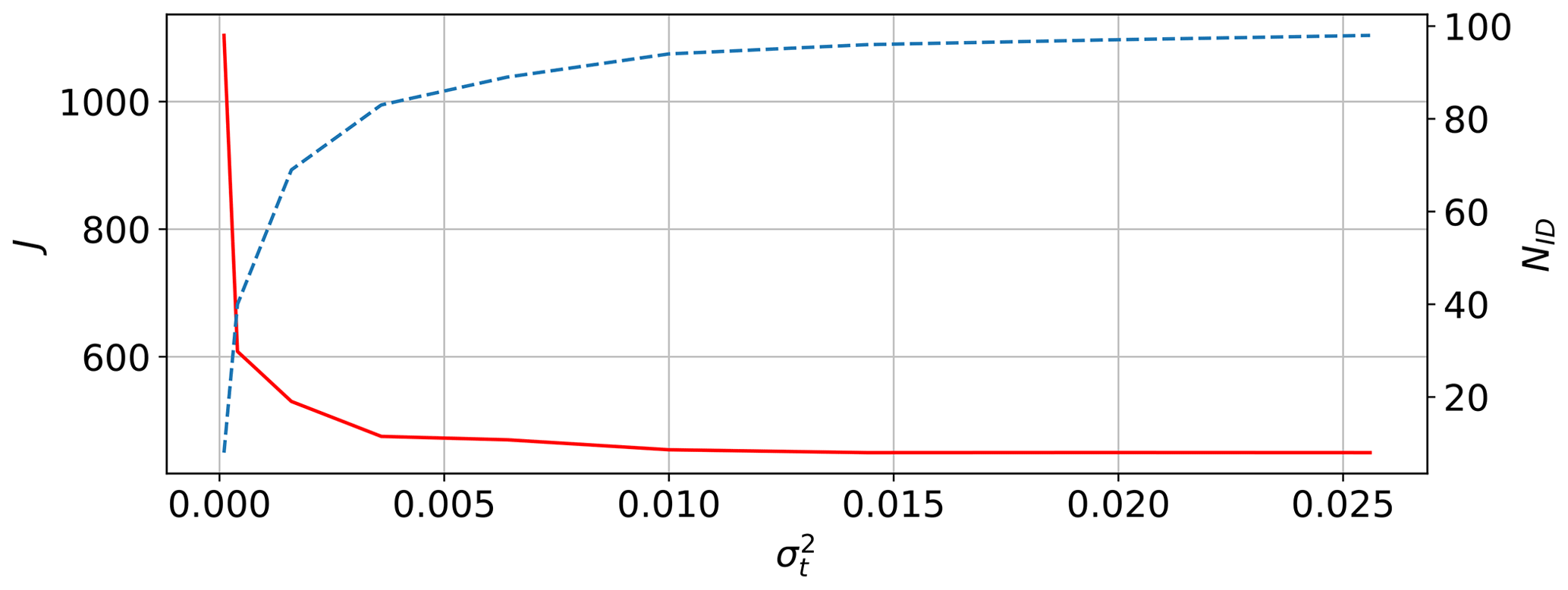
Figure 3 Likelihood cost function J (solid red line) and number of retained parameters N_ID (dashed blue line) as functions of ${\mathit{\sigma }}_{\mathrm{t}}^{\mathrm{2}}$.

The STL parameter vector p was defined as follows.

• For the data-driven learning of the heterogeneous background velocity ΔU=ΔU_STL, a north-oriented, regular mesh of 5×7 flow correction nodes was superimposed onto the farm (see Fig. 3a). The node spacing is 470 m and 450 m in the eastern and northern directions, respectively. It was verified that a finer spatial discretization did not improve the quality of the results. An additional discretization of the environmental conditions A₀ (see Eq. 7) was performed only for wind direction. To this end, a second set of nodes was placed every 15^∘, i.e., for the distinct values ${\mathrm{\Gamma }}_{\mathrm{0}}\in [\mathrm{255},\mathrm{270},\mathrm{285},\mathrm{300}]$^∘. Results indicated that the relative correction $\mathrm{\Delta }U/U_{\mathrm{0}}$ does not change significantly depending on wind speed. This suggests that the terrain flow is Reynolds independent, as often assumed in over-the-terrain CFD application (van der Laan et al., 2020). Therefore, each nodal correction parameter p_U,i was treated as a non-dimensional speedup factor, independently of the inflow wind speed. To accommodate this change, Eq. (4) was re-written as

  $$\begin{array}{}\text{(27)}& U=U_{\mathrm{0}}\left(\mathrm{1}+\mathrm{\Delta }\widehat{U}\right)+\mathrm{\Delta }{U}_{\mathrm{wake}},\end{array}$$

  where $\mathrm{\Delta }\widehat{U}=\mathrm{\Delta }U/U_{\mathrm{0}}$ is now a relative correction. The term I₀ was also found to have no significant influence on the results and was therefore omitted from the dependencies of the flow speedup. According to these choices, the heterogeneous background velocity was discretized using 140 unknown nodal values p_U. The relative speedup bounds were set to ±0.3, i.e., the corrections can change the reference speed by ±30 %.

• Although orography-induced effects may in principle result in the heterogeneity of the wind direction at a site, such an effect could not be observed at Sedini based on the available dataset. On the other hand, a global correction of the wind direction proved to be necessary and very beneficial for the quality of the results. This was achieved by using a single correction node p_Γ in Eq. (8), without any assumed dependency on A₀. This resulted in a shift in the wind direction, constant throughout the entire farm area and independent of the ambient conditions, which was learned from the operational data of the turbines. It was not possible to clarify with certainty the root reason for this offset, which is probably due to some problem with the yaw sensors.

• The identification of a heterogeneous TI field ΔI was omitted because the available SCADA data did not contain 10 min power min and max values (sometimes used as a proxy for TI (Mittelmeier et al., 2017)) nor other information that could be used for this purpose.

• The wake model behavior is captured by the wake parameter vector p_W, which includes the four velocity parameters α, β, k_a, and k_b, and the four turbulence parameters I_constant, I_ai, I_initial, and I_downstream. The wake model parameters were tuned within the range ±k_init, simultaneously to the learning of the flow correction parameters p_U and p_Γ.

These choices led to the definition of the unknown parameter vector $\mathit{p}=[{\mathit{p}}_U,p_{\mathrm{\Gamma }},p_{\mathrm{W}}{]}^{\mathrm{T}}$, resulting in a total of N_p=149 to-be-identified parameters.

The error covariance matrix was assumed to be known a priori and diagonal, i.e., $R_{i,j}={\mathit{\sigma }}_{\mathrm{m}}^{\mathrm{2}}{\mathit{\delta }}_{i,j}$, where δ_i,j is the Kronecker delta. This assumption can be eliminated by estimating the covariance from the residuals and iterating until convergence (Jategaonkar, 2006), although this did not significantly improve the results in the present case. The cost function expressed by Eq. (15) was selected as

$$\begin{array}{}\text{(28)}& J\left(\mathit{p}\right)={\displaystyle \frac{\mathrm{1}}{\mathrm{2}}}\sum _{i=\mathrm{1}}^N{w}_i{\mathit{r}}_i^{\mathrm{T}}\mathbf{R}{\mathit{r}}_i,\end{array}$$

where the factors w_i are proportional to the number of 10 min observations within each bin in order to weight their participation based on the number of samples that they contain. The solution procedure was based on first applying the SVD, thereby recasting the STL parameters into the orthogonal set θ. After discarding the orthogonal parameters whose variance fell above the observability threshold, the optimization was run with the sequential least squares programming (SLSQP) minimization algorithm, as implemented in the SciPy library (Virtanen et al., 2020). This process was repeated multiple times (three in the two examples below) to ensure convergence, as expressed by changes in the singular values s_i.

The choice of the observability threshold ${\mathit{\sigma }}_{\mathrm{t}}^{\mathrm{2}}$ for the orthogonal parameters was based on an analysis of its effects on the likelihood cost function J and number of retained parameters N_ID. The results are shown in Fig. 3, which reports J (with a solid red line) and N_ID (with a dashed blue line) as functions of ${\mathit{\sigma }}_{\mathrm{t}}^{\mathrm{2}}$. As expected, an increasing threshold has the effect of retaining a larger number of parameters in the identification. This leads to an improvement in the likelihood function, but it also comes with an increased computational cost. In fact, the execution time was about [1, 6, 12] h for ${\mathit{\sigma }}_{\mathrm{t}}^{\mathrm{2}}=[\mathrm{0.016},\mathrm{0.01},\mathrm{0.02}]$, respectively, on a 2019 Intel^® Core™ i7-9700 CPU desktop. However, it should be noted that processing time is not a very meaningful metric because the present code was not optimized for speed and processing power improves rapidly over time, quickly rendering execution times obsolete. Figure 3 also shows that the J vs. ${\mathit{\sigma }}_{\mathrm{t}}^{\mathrm{2}}$ curve exhibits a “knee” around the values 0.02–0.03: below these values small increments of ${\mathit{\sigma }}_{\mathrm{t}}^{\mathrm{2}}$ lead to large reductions in J, whereas above only very marginal further improvements are possible. This indicates that the additional parameters that are retained in the solution in reality do not carry any significant additional informational content. The results discussed in the following correspond to the case ${\mathit{\sigma }}_{\mathrm{t}}^{\mathrm{2}}=\mathrm{0.01}$, although nearly identical conclusions are obtained for the looser values around and after the curve knee.

Figure 4 shows the distribution of the variance of the orthogonal parameters, i.e., the squared inverse of the singular values, before the third and last run of the MLE algorithm. Of the 149 orthogonal parameters, N_ID=94 had a variance below the threshold and were retained in the optimization; the number of retained parameters was constant throughout the iterations. The same figure shows that 24 parameters exhibit extremely high variances. These parameters are associated with flow correction nodes that lie outside of the perimeter of the farm; since the identification process is purely driven by data that are co-located with the turbines, the parameters associated with these farm-external nodes carry very little information and hence have very high variance. The informational content of the retained singular values can be estimated as $\mathit{\varphi }=\sum _{i=\mathrm{1}}^{N_{\mathrm{ID}}}{s}_i^{\mathrm{2}}/\sum _{i=\mathrm{1}}^{N_{\mathrm{p}}}{s}_i^{\mathrm{2}}=\mathrm{97}$ % (Jolliffe and Cadima, 2016).

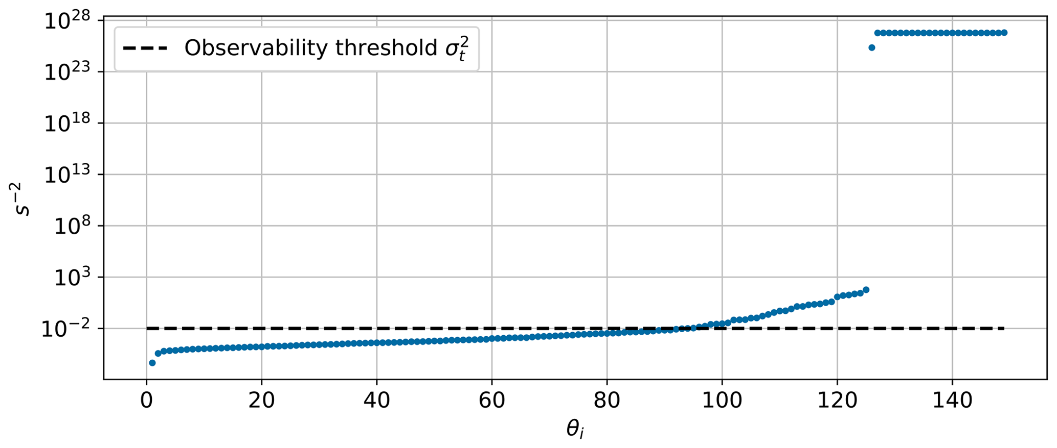
Figure 4 Variance of all orthogonal parameters θ_1–149 before the last MLE. Only 94 parameters were retained in the identification, whereas the others above the variance threshold (indicated with a dashed black line) were discarded.

3.1.3 Results for wind direction correction and wake model tuning

As previously mentioned, the wind direction was corrected over the entire domain by the value ΔΓ=5.6^∘, suggesting that the average yaw sensor readings are affected by an offset. The exact reason for such a large difference could not be ascertained and might be due to a combination of factors, including the small number of turbines with acceptable yaw signals (just eight), possible miscalibrations of the sensors, and the manually performed correction of drift and biases based on wake interactions. In this sense, the ability of the STL approach of automatically finding the optimal correction appears to be very useful, since sensor biases – especially in the yaw drives – are a common challenge (Bromm et al., 2018).

Table 2 reports the results of the wake model tuning. According to Eq. (11), the initial baseline values k_init are summed to their respective correction parameters p_k to yield the final, tuned model parameters k. The extent of the near-wake region is determined by α and β, while k_a and k_b model the wake expansion in the far region (Bastankhah and Porté-Agel, 2016). Examining the relative parameter changes, reported in the last row of the table, it appears that α – which models the influence of turbulence intensity on the downstream extension of the near wake – is the term that changed the most. With the present tuning, for an ambient I₀=0.14, the near wake is 28 % shorter than with the initial baseline values. With an earlier start of decay, the far wake deficit is reduced. As a result, a downstream turbine operating at about 3 D (the typical distance for the Sedini farm) produces 42 % more power, thereby significantly decreasing the wake losses predicted by the baseline tuning. Furthermore, the wakes have a higher sensitivity to the different day and night ambient turbulence intensity than before. On the other hand, tuning led to an only marginal increase in the added turbulence model.

Table 2 Results of the wake model tuning, with the initial baseline parameters k_init, the identified values of the additive corrections p_k, and the final tuned parameters k. The last row reports the relative change from k_init to k.

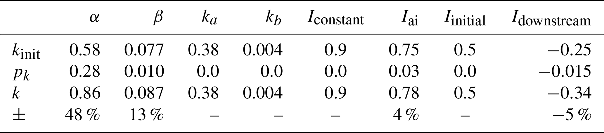
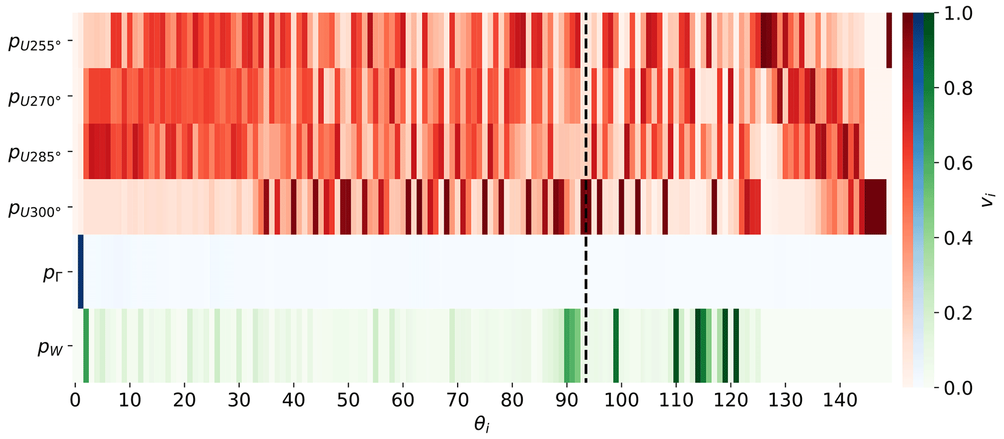
Figure 5 Matrix V of reduced singular vectors, ordered by the corresponding orthogonal parameters θ_1–149. The reduced vectors are obtained by taking the root sum of squares of the rows of each row-block partition (corresponding to each different parameter type). The different colors represent the different correction categories: wind speed correction (red), wind direction correction (blue), and wake model tuning (green). The dashed black line indicates the cutoff at i=94, corresponding to the observability threshold σ_t (see Fig. 4).

3.1.4 Orthogonal decomposition

An examination of the rotation matrix V can give some useful insight into the relative importance and correlation of the physical parameters. For a simpler visualization, the large $\mathbf{V}\in {\mathbb{R}}^{N_{\mathrm{p}}\times N_{\mathrm{p}}}$ matrix was condensed in a way that tries to capture the effects of the various types of corrections. According to Eq. (12), the overall parameter vector p is obtained by stacking the different correction parameter vectors, which induces an identical row-block partitioning of V, i.e.,

$$\begin{array}{}\text{(29)}& \mathbf{V}=\left[\begin{array}{c}{\mathbf{V}}_U\\ {\mathbf{V}}_{\mathrm{\Gamma }}\\ {\mathbf{V}}_W\end{array}\right]=\left[\begin{array}{c}{\mathbf{V}}_{U\mathrm{255}{}^{\circ }}\\ \mathrm{⋮}\\ {\mathbf{V}}_{U\mathrm{300}{}^{\circ }}\\ {\mathbf{V}}_{\mathrm{\Gamma }}\\ {\mathbf{V}}_W\end{array}\right].\end{array}$$

In the third term of the previous expression, V_U has been further partitioned by the directional bins. By definition, each singular vector, i.e., each column v_i of matrix V, has unit length, i.e., $\left|{\mathit{v}}_i\right|=\mathrm{1}$. A visual representation of the matrix that captures the overall contribution of each parameter type was obtained by taking the root sum of squares of each row-block partition. The resulting reduced matrix is visualized in Fig. 5, where the columns are sorted in descending order of the associated singular values. The vertical dashed line represents the cutoff at 94 retained parameters (generated by the observability threshold), which divides V_ID and V_NID, i.e., the identifiable from the non-identifiable orthogonal parameters.

Inspection of the reduced matrix suggests a few observations. First, the directional correction p_Γ, which applies a constant offset throughout the farm, is almost exclusively contained in the first singular vector. Since this bias affects every turbine over the entire dataset, it has a prominent position in the decomposition and is essentially uncoupled from the other parameters. The wake model tuning parameters appear immediately behind the wind direction in the ranking, and they are also highly uncoupled from the rest. An examination of the individual rows of this block (not visible in the figure) shows that the largest contributions come from the k_a and α parameters, as already shown in Table 2. The observability of these parameters improved by introducing the day and night variability in I₀, as previously explained. Finally, the appearance of velocity corrections in the singular vectors seems related not only to the heterogeneity of the flow but also to the number of available observations. In fact, the largest number of data points is available around 270 and 285^∘, whereas data are more sparse around 300^∘, which results in flow correction parameters with lower observability.

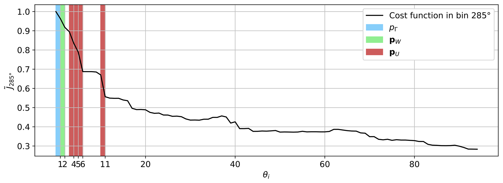
Figure 6 Decrease in the normalized subsector cost function when activating one orthogonal parameter at a time in the sequence θ_1–94. The red-shaded areas represent the flow speedup corrections that contribute the most to the error reduction. The corresponding eigenshapes are visualized in Fig. 7.

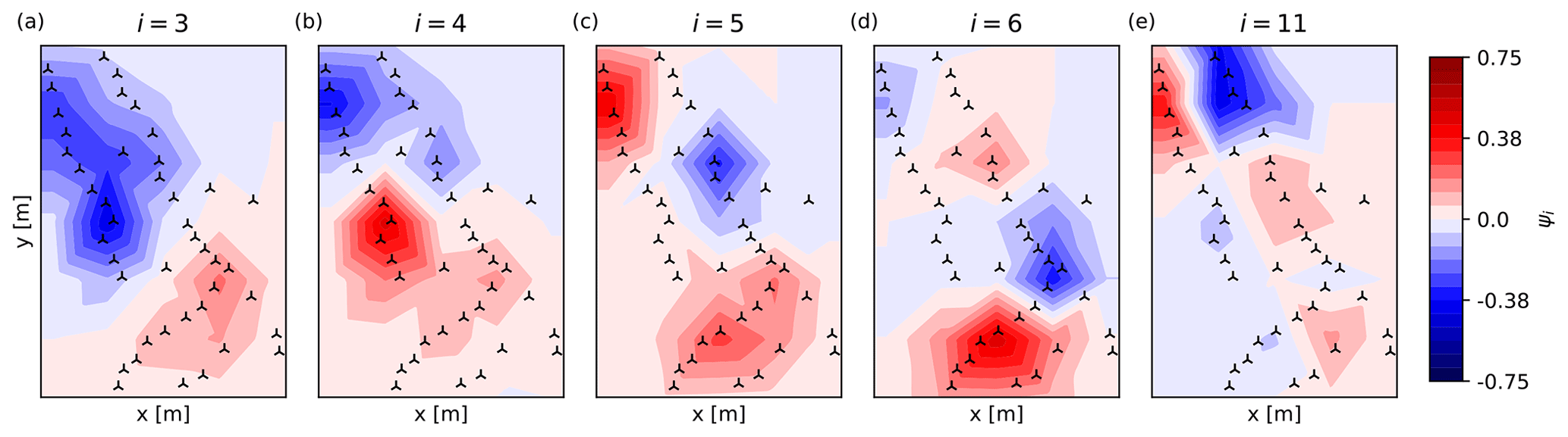
Figure 7 Dominating eigenshapes of the flow corrections ΔU in the $\mathrm{285}{}^{\circ }\pm \mathrm{10}{}^{\circ }$ sector. With increasing counter i (i.e., singular value), corrections become more fragmented, i.e., spatially localized.

To better understand the nature of the corrections ΔU, the singular vectors can be mapped to the farm domain via their shape functions. This is obtained by combining Eq. (8) with Eq. (24) to yield

$$\begin{array}{}\text{(30)}& \mathrm{\Delta }U={\mathit{n}}^{\mathrm{T}}{\mathit{p}}_U\approx {\mathit{n}}^{\mathrm{T}}{\mathbf{V}}_{U,\mathrm{ID}}{\mathit{\theta }}_{\mathrm{ID}}={\mathbf{\Psi }}_U^{\mathrm{T}}{\mathit{\theta }}_{\mathrm{ID}},\end{array}$$

where Ψ is the matrix of eigenshapes (Bottasso et al., 2014). To facilitate the visualization of the eigenshapes, the discussion is restricted to the small sector of $\mathrm{285}{}^{\circ }\pm \mathrm{10}{}^{\circ }$. Figure 6 shows the relative decrease in the cost function (evaluated only in the subsector of $\mathrm{285}{}^{\circ }\pm \mathrm{10}{}^{\circ }$), when activating one orthogonal parameter at a time. As already stated, the first reduction (blue shade in the figure) can be attributed almost exclusively to the directional correction p_Γ. Likewise, the second orthogonal parameter contains mostly corrections to the wake model (green shade). The parameters appearing after the wake model corrections are associated with flow speed corrections. For this subsector, parameters θ_4–6 and θ₁₁ are the most effective ones in reducing the cost function. They account for ca. 41 % of the final cost function improvement and, therefore, are responsible for removing the largest heterogeneous flow discrepancies. An inspection of Fig. 5 shows that, for the row corresponding to ${\mathit{p}}_{U,\mathrm{285}{}^{\circ }}$, the indices of these parameters are indeed associated with a large contribution to the matrix of singular vectors. The cost function is essentially flat for the orthogonal parameters associated with directions outside of the subsector. For example, this is clearly the case for θ_7–10 (corresponding to ${\mathit{p}}_{U,\mathrm{255}{}^{\circ }}$).

Figure 7 finally shows the red-shaded eigenshapes i=4–6, 11 superimposed onto the farm map. In addition to these dominating modes, the figure also reports the lowest flow-related eigenshape (corresponding to i=3), although its cost function improvement is only modest (see Fig. 6). Each eigenshape is multiplied by the sign of the corresponding orthogonal parameter, i.e.,

$$\begin{array}{}\text{(31)}& {\mathit{\psi }}_i={\mathit{v}}_i^{\mathrm{T}}\mathit{n}\mathrm{sign}\left({\mathit{\theta }}_i\right),\end{array}$$

to show speedup and slowdown corrections in a consistent manner.

The first eigenshape, Fig. 7a, represents a roughly north–south speed change. Comparing this plot to the terrain map of Fig. 2 shows that the ground elevation in the northern part of the farm is lower than in the south. As elevated regions generally induce higher velocities, this lowest mode captures this prominent orographic effect of the site. The higher-order eigenshapes become increasingly fragmented and seem to model specific localized terrain features. For example, ψ₄ (see Fig. 7b) captures the very prominent hill in the middle of the western row.

3.1.5 Plausibility check via CFD

The corrections identified by the proposed method describe a direction-dependent heterogeneous flow field that very significantly improves the matching of the FLORIS model predictions with measured operational data. However, is this identified flow field a reasonable approximation of the true flow over the terrain at this site, or is it just a mathematical correction that happens to improve the results? A definitive answer to this question is probably difficult to give with the limited data and information available. However, a qualitative and quantitative verification of the plausibility of the data-learned field can be obtained by comparing it with an independent CFD simulation of the flow over the terrain.

To perform this plausibility check, Reynolds-averaged Navier–Stokes (RANS) simulations were conducted for the values ${\mathrm{\Gamma }}_{\mathrm{0}}\in [\mathrm{255},\mathrm{270},\mathrm{285},\mathrm{300}]$^∘ without the turbines and in neutral atmospheric conditions. The resulting flow fields represent direction-dependent steady-state heterogeneous flows over the terrain, which can be directly compared with the data-driven learned corrections. In principle, the latter also contain intra-plant effects induced by the turbines, which are not present in the former; however, as mentioned in Sect. 3.1.1, given the small streamwise extent of the Sedini farm for this sector, ΔU_wake→amb effects are probably very small and hence negligible. As previously stated, the flow is assumed to be Reynolds-independent, and corrections are expressed in the form of non-dimensional speedup factors. The absolute velocity field was extracted from the computed flow field at hub height (65 m) and then normalized by the average speed at the free-stream turbine locations. A more complete description of the setup of the RANS simulations is provided in Appendix A. Clearly, the CFD results should not be considered a ground truth, since no measurement of the actual flow is available.

To quantify the similarity between the learned and CFD-computed fields, their spatial correlation is calculated as

$$\begin{array}{}\text{(32)}& {\mathit{\varrho }}_{\mathrm{CFD}}={\displaystyle \frac{\mathrm{cov}\left(\mathrm{\Delta }{\stackrel{\mathrm{̃}}{U}}_{\mathrm{STL}}\left(Q\right)\mathrm{\Delta }{\stackrel{\mathrm{̃}}{U}}_{\mathrm{CFD}}\left(Q\right)\right)}{\sqrt{\mathrm{var}\left(\mathrm{\Delta }{\stackrel{\mathrm{̃}}{U}}_{\mathrm{STL}}\left(Q\right)\right)\mathrm{var}\left(\mathrm{\Delta }{\stackrel{\mathrm{̃}}{U}}_{\mathrm{CFD}}\left(Q\right)\right)}}}.\end{array}$$

Ideally, for a perfect match between learned and simulated fields, their spatial correlation ϱ_CFD should be equal to 1. Similarly, a terrain correlation measure is defined as

$$\begin{array}{}\text{(33)}& {\mathit{\varrho }}_{\mathrm{T}}={\displaystyle \frac{\mathrm{cov}\left(\mathrm{\Delta }{\stackrel{\mathrm{̃}}{U}}_{\mathrm{STL}}\left(Q\right)h\left(Q\right)\right)}{\sqrt{\mathrm{var}\left(\mathrm{\Delta }{\stackrel{\mathrm{̃}}{U}}_{\mathrm{STL}}\left(Q\right)\right)\mathrm{var}\left(h\right(Q\left)\right)}}},\end{array}$$

which attempts to quantify the similarity between the elevation h and the learned field $\mathrm{\Delta }{\stackrel{\mathrm{̃}}{U}}_{\mathrm{STL}}$. Ideally, if all speedups were learned exactly and were only due to the terrain elevation, ϱ_T would be equal to 1. Both correlation coefficients are given in Table 3 for the four considered wind directions.

Table 3 Spatial correlation of learned and CFD-computed velocity speedups (ϱ_CFD) and of learned speedups and terrain elevation (ϱ_T) for each considered wind direction.

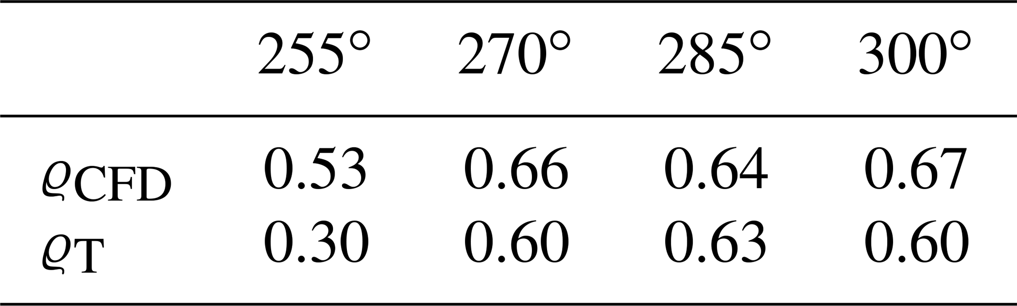
Figure 8 shows the learned (left) and CFD-computed (right) speedup fields for the considered directions of 255, 270, 285, and 300^∘. Looking at the figure, it appears that there is a general agreement on the location of low- and high-speed regions. This qualitatively similar visual appearance is confirmed by the quantitative measure provided by the correlation coefficient ϱ_CFD, which is in the range of 0.53–0.67 for all directions. A comparison with the terrain map of Fig. 2 shows that elevated and depressed regions of the terrain are coherent with flow speed slowdowns and speedups. This suggests that the terrain elevation is the main driver of the identified corrections. The correlation ϱ_T between velocity speedups and terrain elevation confirms this impression, except for the 255^∘ direction. This might be due to the small number of samples for this direction (see the wind rose in Fig. 2) and possibly also to the particularly complex orography upstream of the farm when the wind blows from 255^∘ (see Fig. A1). The STL method seems to estimate more pronounced flow inhomogeneities than CFD. For example, this can be seen for the hill at the southern end of the farm and for the lower-speed region in the northern end. Additionally, the flow pattern in the northern region for the direction of 285^∘ (Fig. 8e) corresponds to the correction introduced in eigenshape i=11 in Fig. 7e. The CFD simulations further show some distinct speedup regions in the center of the farm, which are caused by small hills. For example, for the 255^∘ direction, the STL method is probably not resolving all flow details correctly. This results from the coarse resolution of the grid and, more importantly, from the distance among turbines – and, thus, from the distance among the measurements that drive learning – in that area. Furthermore, the extrapolation of the STL results outside of the farm perimeter cannot work well beyond a short distance because of a lack of information in the data that drive the learning process. Notice, however, that, from the point of view of the quality of the FLORIS model predictions, the lack of knowledge of the flow outside of the farm is of no importance as long as the inflow on the upstream turbines is correctly captured.

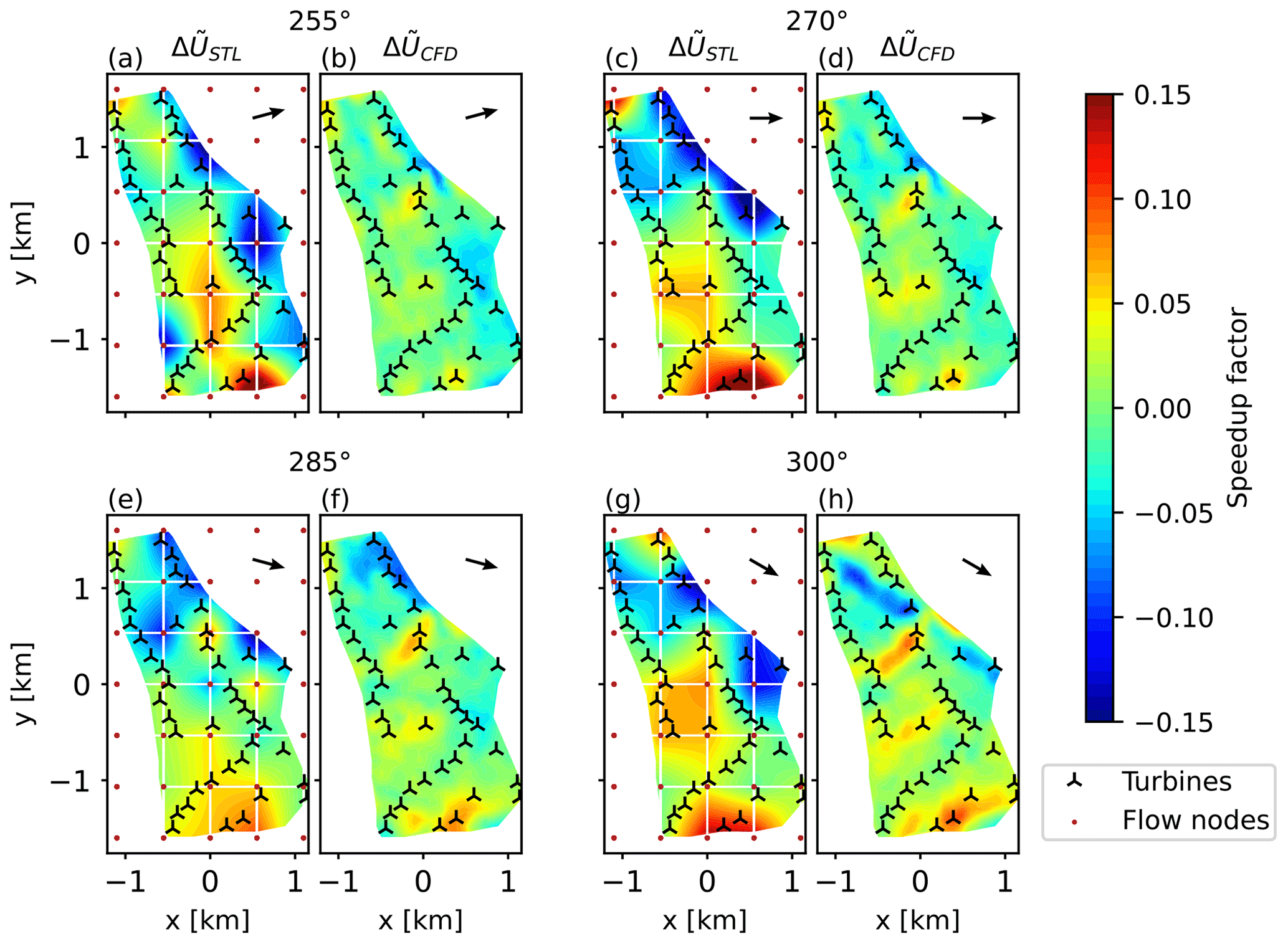
Figure 8 Comparison between the learned (a, c, e, f) and CFD-computed (b, d, f, h) speedup factors for directions of 255, 270, 285, and 300^∘. The learned results are corrected by the identified directional offset ΔΓ.

3.1.6 Initialization of STL by a CFD-computed field

Corrections can be learned with respect to an initial heterogenous flow field, instead of a uniform one (i.e., utilizing Eq. 9 instead of Eq. 8). To verify whether these better initial conditions can lead to improved results, the RANS CFD simulations were used to initialize the background flow, thereby providing a non-uniform baseline solution; in this case, the role of the data-driven corrections is that of compensating any remaining discrepancies. The CFD-computed speedup factors for a generic wind direction were obtained by linear interpolation between the two adjacent simulated directions. The same definition of the flow correction nodes employed in the previous case was used here too.

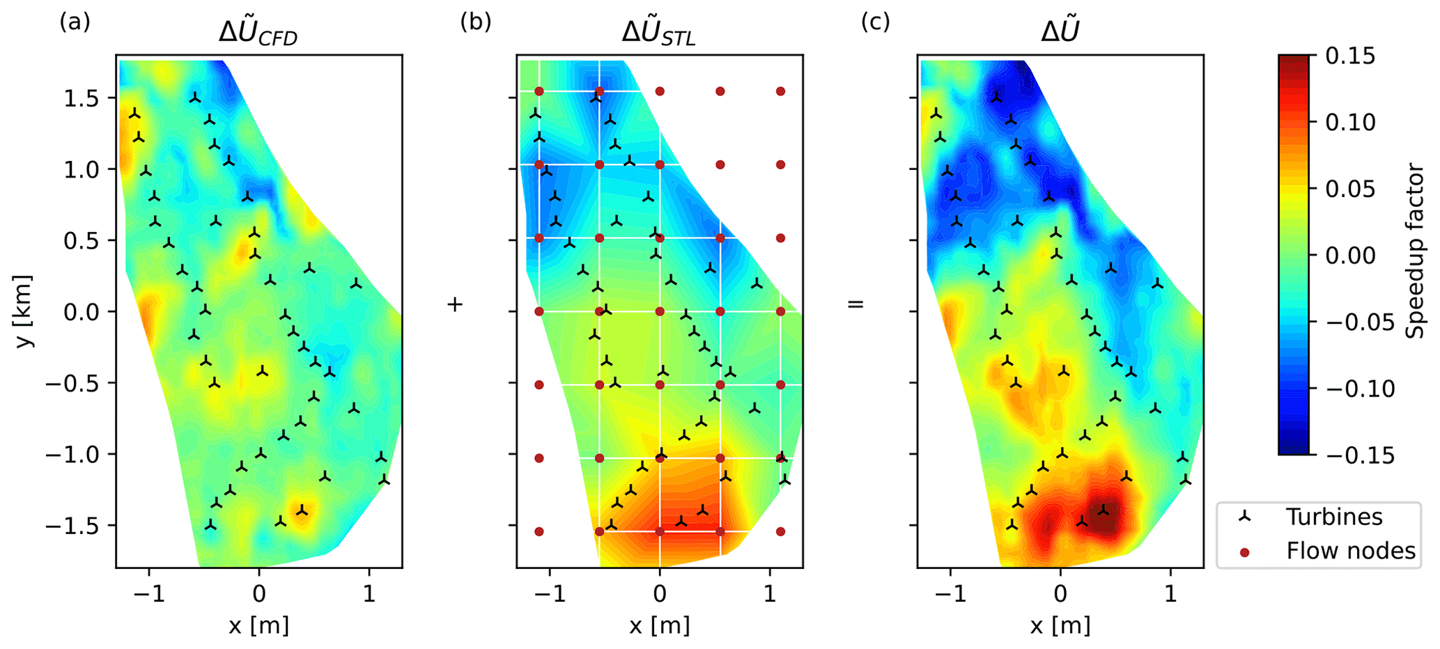
Figure 9 Initial CFD-computed heterogeneous flow (a), data-driven learned correction field (b), and final resulting flow field (c). All results are for the 270^∘ wind direction.

Results indicate that the identified wind direction p_Γ and wake p_W parameters (see Sect. 3.1.3) were not affected by the improved initial background flow. Figure 9 shows, for the 270^∘ direction case, the CFD initial baseline solution (Fig. 9a), the learned corrections (Fig. 9b), and the final heterogeneous velocity field (Fig. 9c). The learned corrections seem in general to increase the initial CFD-computed terrain inhomogeneities.

As shown in the next section, the use of a CFD-computed initial flow field offers quantitatively no visible error reduction for power when compared to the simpler option of starting from an initial uniform background flow. Indeed, the solution shown in Fig. 9c is very similar to the one of Fig. 8c, while the direction and wake correction parameters are also essentially identical. As a consequence, the turbine inflows, where the error is computed, are very similar. However, the CFD-based approach allows for a finer resolution of the flow field in between the turbines and externally to the farm perimeter. In addition, the fact that essentially the same solution is obtained for very different initial conditions seems to indicate the absence of distinct local minima, at least for this case.

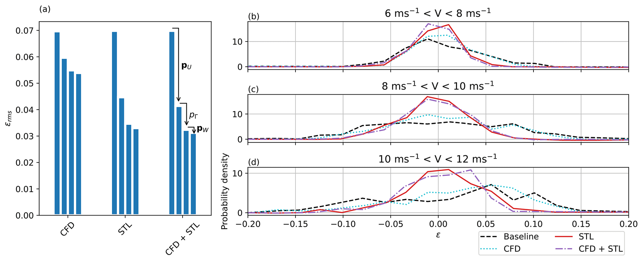
Figure 10 Reduction in the overall error by the activation of different correction types (a). Error probability density distribution for different wind speed ranges (b–d).

3.1.7 Contributors to the error improvement

At the convergence of the estimation process, the remaining error is defined as

$$\begin{array}{}\text{(34)}& \mathit{ϵ}={\displaystyle \frac{P_{\mathrm{SCADA}}-P_{\mathrm{model}}}{P_{\mathrm{rated}}}},\end{array}$$

where P is the overall farm power, and the error is calculated only using the test part of the dataset, i.e., discarding the data points used for learning. Four cases of increasing complexity were compared, as listed in Table 4. In the baseline case, the FLORIS model is used without any correction, i.e., using a homogeneous background flow, no wind direction correction, and wake-describing parameters sourced from the literature. In the case labeled “CFD”, the background flow is the one computed with the RANS model without additional data-driven corrections; in this case, learning is limited to the wind direction and the tuning of wake-describing parameters. In the case labeled “STL”, the initial background flow is uniform, and learning is used to compute the full heterogeneity of the flow, in addition to direction and wake behavior. Finally, in the case labeled “CFD + STL”, the initial background flow is the RANS-computed one, and learning is used to further correct this already heterogeneous field, in addition to direction and wake behavior.

Table 4 Four different cases for the analysis of learned corrections on the power matching error.

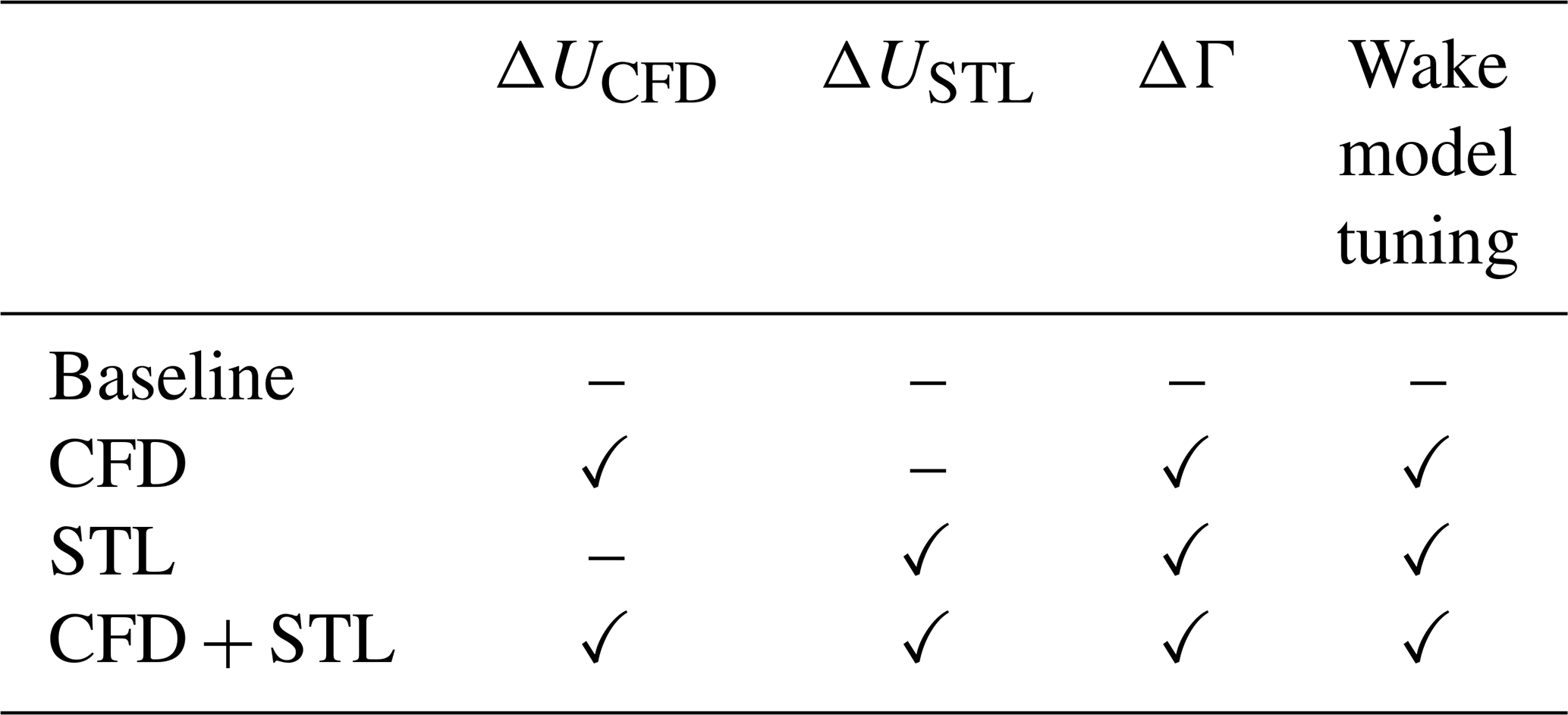
Figure 10 gives an overview of the error reduction that can be achieved compared to the baseline performance. Figure 10a shows the impact of each different correction type on the overall error ${\mathit{ϵ}}_{\mathrm{rms}}=\sqrt{\mathrm{1}/N_{\mathrm{test}}\sum {\mathit{ϵ}}_i^{\mathrm{2}}}$. For all considered cases, the addition of a heterogeneous velocity field resulted in the most substantial error improvement. As expected, the error for the CFD case is larger than in the cases when the background flow is learned or corrected; in fact, since the CFD results are not aware of any on-site measurements, they are probably not completely accurate and representative of the actual terrain-induced inhomogeneities. The final error for the STL and CFD+STL cases is extremely similar, showing that – notwithstanding the different initial conditions – the solution is essentially the same. The identified directional offset was similar in all three cases and thus decreased the error in the same manner. Given the strong effects caused at this site by the terrain-induced flow heterogeneity and the significant direction bias, the wake model tuning accounted only for a relatively small improvement in the error.

Figure 10b through d show the probability distribution of the errors for three binned wind speed regimes. The FLORIS baseline model tends to overpredict power production for low wind speeds and to underpredict it for high wind speeds. Using STL, this effect is eliminated, and the error spread is significantly improved. As already noticed, STL and CFD + STL cases achieve very similar error distributions.

Figure 11 (as well as the larger Figs. B1 and B2) gives a more detailed insight in the learned corrections. The figures show the 5^∘ binned measurements and calculated power per turbine in the sector of 245–310^∘ for the wind speed range of $U_{\mathrm{0}}\in [\mathrm{6},\mathrm{8}]$ m s⁻¹.

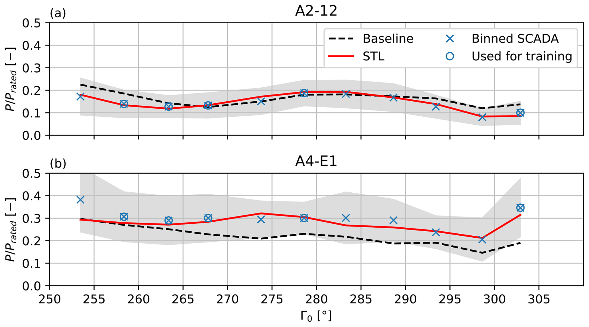
Figure 11 Normalized measured and calculated power for the two turbines A2-12 (a) and A4-E1 (b) for all 5^∘ bins in the investigated western sector for wind speeds in the range of 6–8 m s⁻¹ during daytime operation. Bins with <10 observations are not shown. Bins used for training are marked with a ∘ symbol. The uncertainty band shows the standard deviation in the bins. The baseline results are calculated without any data-driven corrections.

Figure 11 focuses on two turbines that clearly highlight the improvements achieved by learning during daytime operation. In particular, turbine A2-12 (Fig. 11a) experiences a distinct wake shading by turbine A5-E5 in the direction range 255–270^∘(see the farm layout shown in Fig. 2). The corrected model matches well the behavior of the measurements, whereas the baseline model is visibly offset on account of the large wind direction bias.

A similar situation is observed for turbine A1-E7 in the general overview plot of Fig. B1. Note that the power drops observed for Γ₀=300^∘ do not originate from wake interactions but are due to a low bin average speed U₀. In fact, not many distinct wake interactions are visible in the plot, as the farm layout was specifically designed for this main wind direction. Some turbines in the western row are even operating in free-stream conditions over the entire dataset; these machines are labeled FS in Fig. B1. The effects of the terrain-induced flow corrections can be clearly appreciated by looking at turbine A5-E5 (Fig. 11b), which is located on a hill that is about 20 m higher than the average elevation of the farm. Without the heterogeneous flow model, FLORIS underestimates the power output of this turbine. However, in the STL case, the hill-induced speedup is captured by the learned corrections. The speedup is also visible at the location of turbine A5-E5 in Fig. 8.

The color of the frames of each subplot of Figs. B1 and B2 shows the elevation difference Δh of the turbine foundations with respect to the farm average. The power of the turbines at the lower elevations is mostly overestimated by the baseline FLORIS, whereas the opposite happens for the turbines at the higher elevations. The learned corrections compensate for these terrain-induced effects, leading to a good overall match throughout the whole plant.

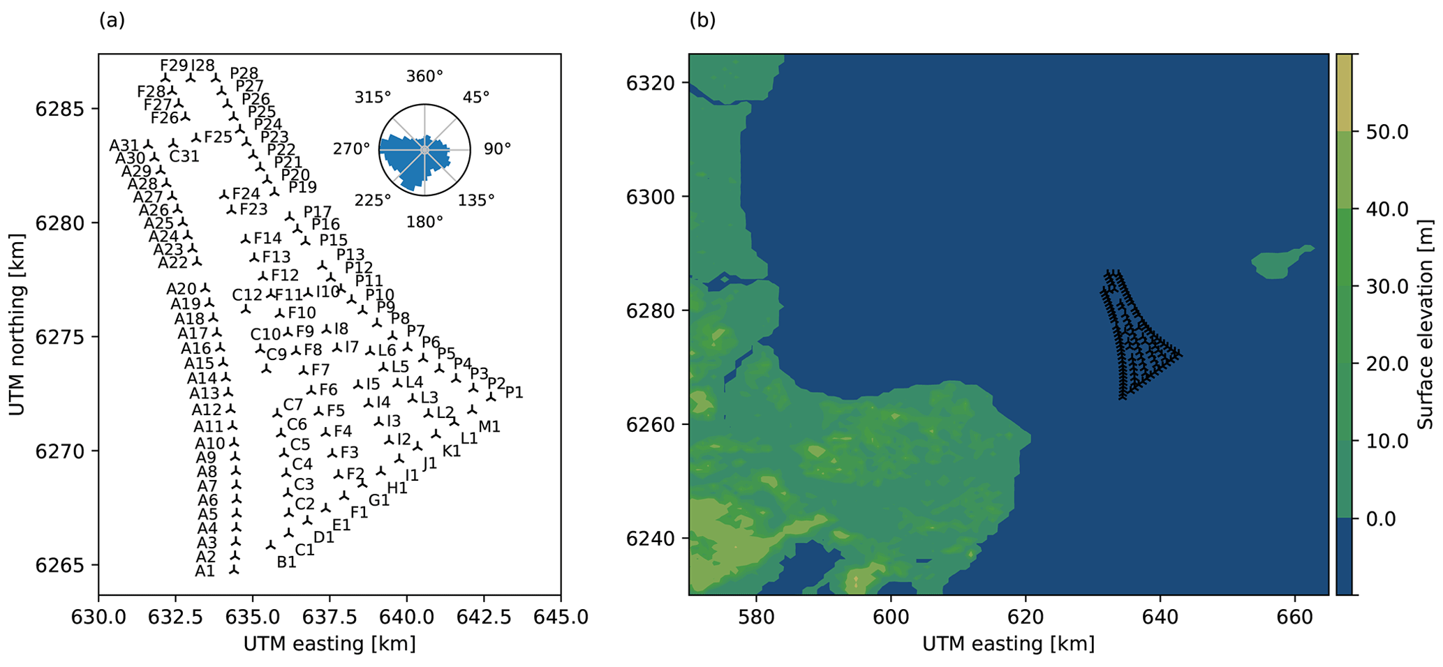
Figure 12 Layout of the Anholt wind farm with turbine identifiers and wind direction frequency (a). Location of the site, including the Jutland peninsula to the west and the island of Anholt to the east (b).

3.2 The Anholt wind farm

3.2.1 Site overview, dataset analysis, and preprocessing

Figure 12b shows the Anholt wind farm, together with its surrounding coastlines. The farm consists of 111 Siemens Gamesa SWT 3.6-120 wind turbines, and it is situated about 20 km east of the Jutland peninsula and about 25 km west of the island of Anholt. The prevailing wind direction at the site is west–southwest. The farm has an irregular spacing, varying between 5 and 12 rotor diameters: the turbines forming the farm perimeter have a close spacing of about 5–6 D, whereas the spacing within the farm is larger.

Tuning and learning were performed using the same procedures as in the Sedini case. However, the two cases are significantly different, impacting the relative importance of the heterogeneous corrections terms of Eq. (5).

• Term ΔU_amb. The fact that Anholt is an offshore farm does not mean that terrain effects are absent. On the contrary, a terrain and roughness-induced velocity variation exists, caused by the land upstream of the site (whereas the effects of changing sea state were not considered). Hence, a heterogeneous velocity field can be identified from the turbine operational data. Similarly to the onshore case, even here a terrain-only CFD simulation provides a qualitative solution for verifying the plausibility of the data-driven corrections.

• Term ΔU_wake→amb. The much larger streamwise depth of the farm increases the importance of plant-induced effects compared to the Sedini case. Such effects are expected to depend on the stability of the atmosphere (Porté-Agel et al., 2020), which here was approximately taken into account by binning based on mesoscale re-analyses.

Since in this case both correction terms are relevant, it is not a straightforward task to disentangle the learned plant-induced corrections ΔU_wake→amb from the ambient ones ΔU_amb. Although more sophisticated approaches are certainly possible, here a simple solution was adopted that consists of comparing the non-uniform inflow caused by the coastline with CFD analysis of the site. For brevity, the analysis of the SVD decomposition performed for Sedini is omitted in this case.

For the present analysis, SCADA data at 10 min sampling frequency were available from January 2013 until July 2015. The overall problem setup, solution methods, and data preprocessing were the same used for the onshore plant, as described in Sect. 3.1. In contrast to the Sedini case, however, the data of the yaw sensors were found to be of a higher quality and consistency. Consequently, after removing yaw jumps and offsets, the ambient wind direction Γ₀ was calculated as the mean of the yaw signals across all turbines. The reference speed was determined by averaging the REWS of the free-stream turbines, computed from the power curve like for the previous case. Furthermore, a constant air density of ρ₀=1.225 kg m⁻³ and a vertical wind shear exponent α₀=0.11 were considered. The wind shear was derived as the average measured at the lidar buoy for unwaked directions. Note that, since all turbines have the same hub height, shear has only a very modest effect on the results. Mesoscale wind climate simulations of the region were carried out by Peña et al. (2018) using the Weather Research and Forecasting model (WRF; Skamarock et al., 2008). The results are in the form of time series of hourly outputs for the years 2013–2015, corresponding to the SCADA time period, with a horizontal resolution of 2×2 km, interpolated at the turbine hub height (81.5 m). The simulations do not include the effects caused by the wind turbines on the boundary layer (Fitch et al., 2012).

In addition to providing a comparison for learned coastline-induced effects, the WRF time series were used to filter the dataset for atmospheric stability. Following Van Wijk et al. (1990), periods with Obukhov lengths in the range $\mathrm{0}<L\le \mathrm{1000}$ were classified as stable, whereas periods with $-\mathrm{1000}\le L<\mathrm{0}$ were labeled as unstable; neutral conditions were defined for |L|>1000. Based on these criteria, 22 % of the time stamps were classified as stable and 64 % as unstable; neutral conditions occurred only 7 % of the time and were therefore not considered further. This dominance of unstable conditions was observed at other Baltic offshore farms, e.g., Rødsand (Motta et al., 2005; Archer et al., 2016).

Unstable and stable observations were separated, creating two distinct datasets. Since turbulence intensity could be not inferred from the available SCADA data, it was assigned based on stability, using I=7.5 % for unstable and I=5 % for stable conditions; these values are based on met-mast measurements at the Horns Rev wind farm, as reported by Hansen et al. (2012). Notice that the diurnal cycle, as utilized at the Sedini site, is not very dominant in offshore conditions (Motta et al., 2005). After filtering, the first dataset consisted of 17 492 unstable 10 min time stamps and the second of 3351 stable ones. Both datasets were grouped and averaged in direction and speed bins, respectively, of 10^∘ and 2 m s⁻¹, resulting in N=108 observations for both sets. Half of the bins were picked at random to form the training dataset, whilst the other half were reserved for testing.

3.2.2 STL parameter identification

The STL parameter vector p was defined as follows.

• Similarly to the Sedini case, the wind speed corrections were defined as Reynolds-independent speedup factors $\mathrm{\Delta }\widehat{U}$, as in Eq. (27), which were discretized over the wind farm area and as functions of wind direction. For the spatial discretization, a north-oriented regular mesh of 4×6 flow correction nodes was superimposed to the farm, as shown in Fig. 1b. Given the expected smoothness and relatively large scale of the intra-plant flow features, the spacing of the nodes is several times larger than for the Sedini case, with node-to-node distances of 4 km in the eastern direction and 4.4 km in the northern one. A grid size convergence study showed this spacing to be dense enough to properly resolve the relevant flow features, while coarse enough for a reasonably fast computing time. Just like for Sedini, wind direction variability was taken into account by using a different spatial set of parameters every 30^∘, for ${\mathrm{\Gamma }}_{\mathrm{0}}\in [\mathrm{0},\mathrm{30},\mathrm{\dots },\mathrm{330}]$^∘. These parameters could have been further discretized in terms of atmospheric stability. However, for practical and computational reasons, the identification was instead performed twice, once considering only stable conditions, and once using only the unstable data points. As a result, each problem was defined by 24 spatially distributed speedup parameters p_U for 12 different wind directions, resulting in a total of 288 to-be-identified parameters.

• For the wind direction, a single parameter p_Γ was chosen, in order to account for any global offset in the wind direction. In fact, heterogeneous wind direction fields over the farm domain were not observable in the available dataset.

• The wake model tuning parameters p_W were chosen as in the Sedini case, with the exception of the near-wake parameters α and β, which were omitted on account of the large turbine spacing.

Based on these choices, the vector of parameters was defined as $\mathit{p}=[{\mathit{p}}_U,p_{\mathrm{\Gamma }},p_{\mathrm{W}}{]}^{\mathrm{T}}$, containing a total of N_p=295 free quantities. The identification was performed with three iterations of orthogonal decomposition followed by MLE. At the last iteration, 211 and 216 orthogonal parameters were retained for the unstable and stable identifications, respectively.

3.2.3 Coastline effects

The influence of the Danish coastline about 20 km west of the Anholt wind plant has already been analyzed by Peña et al. (2018) and van der Laan et al. (2017). In particular, the former reference investigated the speed gradients that can be observed for westerly winds, by comparing SCADA data with WRF simulations. Here, this comparison is instead performed with the heterogeneous corrections learned by the STL method. To capture only coastline effects, it is useful to exclude plant-induced effects as much as possible from the analysis. To this end, the comparison is performed considering only the front row of turbines for the unstable dataset, as in this case the term ΔU_wake→amb plays a lesser role. The WRF simulation results were filtered for stability with the same criteria used for the field data and are denoted WRF_unstab.

Figure 13 shows the WRF-computed speedup field generated from all situations where the wind direction is $\mathrm{240}{}^{\circ }\pm \mathrm{5}{}^{\circ }$. Speedups were computed with respect to the average speed measured at the freestream turbines (marked in red), similarly to the STL case. The figure clearly indicates the presence of a wind speed gradient in the inflow of the wind farm, resulting from the wake of the Jutland peninsula. For the wind rotating to the northwest, the wake of the peninsula shifts more towards the southern edge of the wind farm, whereas the opposite happens for wind rotations towards the southwest.

Figure 13 WRF-computed (Peña et al., 2018) wind speedup field in proximity to the Anholt site for wind directions of $\mathrm{240}{}^{\circ }\pm \mathrm{5}{}^{\circ }$ at hub height in unstable conditions without considering the wind turbines. The speedup factors refer to the front row average. The coordinate direction η is always perpendicular to the wind direction, originating at turbine A01.

Figure 14 shows the speedup factors for the western wind directions of 240, 250, 260, and 270^∘. Two sets of speedups are reported in the figure: the simulated ones, which are labeled WRF_unstab and were obtained by interpolating the simulated flow field along the front row of turbines, and the identified ones, labeled STL_unstab and computed by interpolating the nodal parameters at the turbine positions and wind direction. As expected, for smaller wind direction angles, the speedups for the southern turbines are below the value of 0, indicating a decrease in inflow speed caused by the wake of the peninsula. As the wind rotates to the north, the wake of the peninsula shifts to the south; eventually, for 270^∘, only the southernmost turbines are affected.

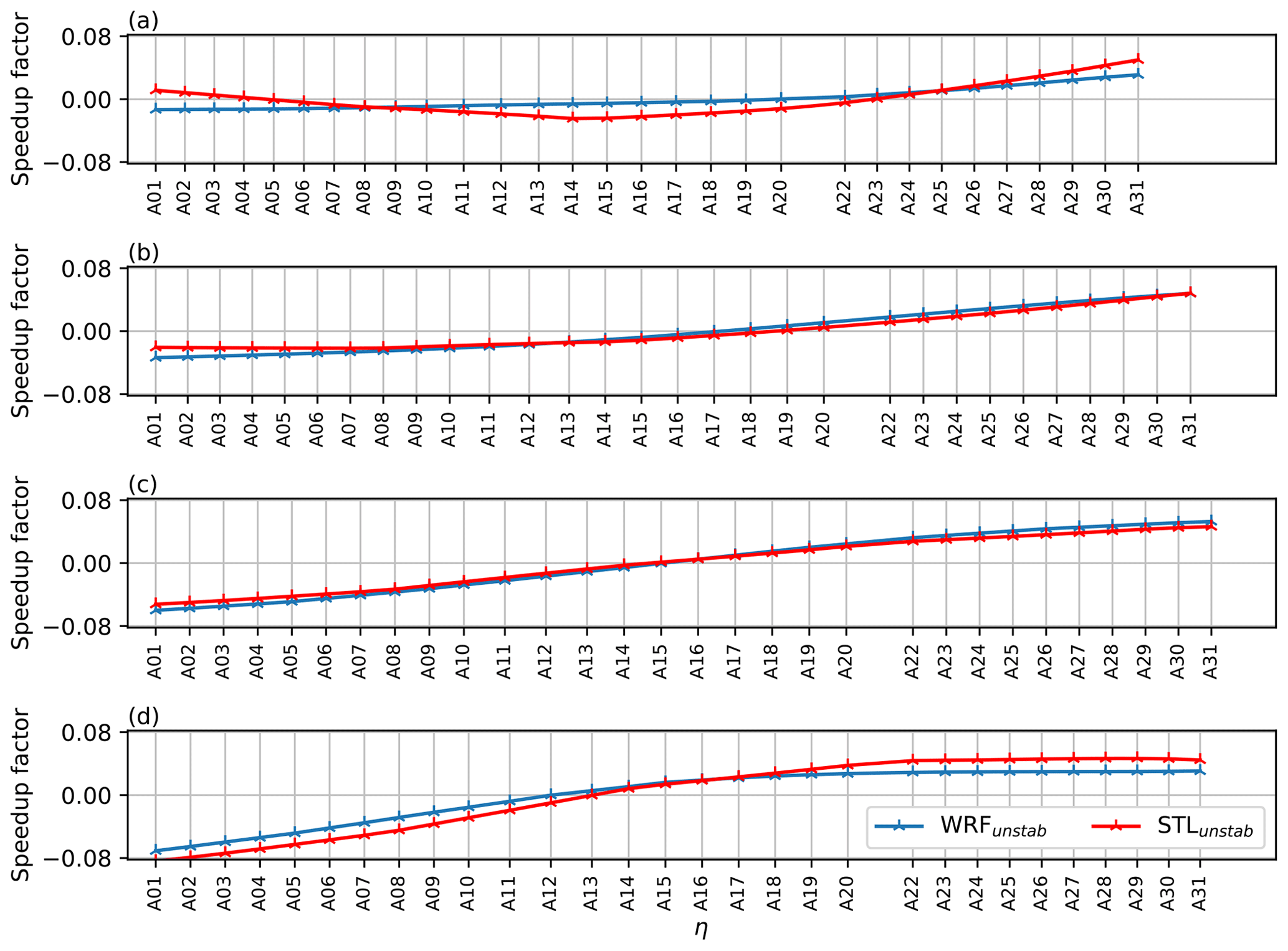
Figure 14 Speedup factors at the first row of turbines for westerly winds from 240^∘ (a), 250 ^∘ (b), 260^∘ (c), and 270^∘ (d). The coordinate η is shown in Fig. 13, and the tick positions are proportional to the lateral distance between the turbines, normal to the wind direction.

The speedup factors from WRF_unstab and STL_unstab are generally in a good agreement. The remaining discrepancies can be explained as follows.

• The speedup factors for STL_unstab were identified for discrete wind directions at intervals of 30^∘. For a given wind direction, the speedup was then linearly interpolated from the identified discrete values. On the other hand, SCADA measurements were binned at intervals of 10^∘, which means that the wind direction dependencies of the two sets of results have different resolutions.

• WRF simulations were run without the presence of the turbines, which therefore cannot include plant-induced effects. On the other hand, STL results are based on measured turbine data, which automatically include such effects.

These results show that the STL method is capable of detecting the inflow heterogeneity at this site. A similar capability was achieved – albeit in a less general setting than here – by Schreiber et al. (2020a), introducing an ad hoc correction field to the inflow of the FLORIS model.

3.2.4 Plant-induced effects

Plant-induced flow effects account for various complex, often interrelated phenomena. At a macroscopic level, a wind farm acts similarly to a local patch of increased surface roughness in its encounter with the atmospheric flow, leading to the development of an internal boundary layer (Porté-Agel et al., 2020). Additionally, wind tends to be “blocked”, i.e., to flow around a farm rather than through it, especially in stable atmospheric conditions; this may lead to significant speed drops within the boundaries of the plant, with consequent power losses (Bleeg et al., 2018). At the same time, as the flow turns around the obstacle represented by the farm, it may locally accelerate close to its edges, resulting in increased local power outputs (Mitraszewski et al., 2013). In stable conditions, wind plants can act similarly to large orographic features such as hills and mountains, resulting in the generation of gravity waves (Teixeira, 2014). This phenomenon likely produces pressure changes in front of and within the wind plant, which can locally negatively or positively affect power capture (Smith, 2010). Individual wind turbines are also responsible for local blockage effects: in fact, in regular arrays, the flow can be channeled in between adjacent rows of turbines, resulting in local streaks of accelerated flow (Abkar and Porté-Agel, 2013).

The present method employs a correction term ΔU_wake→amb to model any flow heterogeneity, irrespective of its originating phenomenon. Such an approach is general and capable of very significantly boosting the quality of the match of the flow model with actual measurements. On the other hand, the drawback is that it may be difficult to disentangle one effect from the other. For example, blockage may affect the production of the turbines, but – presumably – gravity waves can also affect production. When these phenomena are present, they will generate a corresponding background flow in the model that captures such effects. However, looking at the identified flow field, it might not be possible to recognize, for example, blockage per se, as one would also need measurements of the wind speed in front of the plant, for example from a lidar, a met mast, or even an isolated upstream wind turbine. In general, multiple concurrent phenomena can be disentangled only if they are driven by different sets of parameters and if one has access to datasets that contain the necessary variability in such parameters. These two conditions might not always be met, and in fact they are not in the present case.

Figure 15 Learned speedup fields for various wind directions for STL_unstab (unstable conditions) and STL_stab (stable conditions), showing different large-scale wind farm effects. The directions 0, 30, 180, and 210^∘ exhibit clear edge and wall effects, where the flow locally accelerates while turning around the farm.

The ability to explain the results of data-driven approaches remains a topic of central importance for future research. A possible way to address this need is to resort once again to a grey-box approach by embedding within FLORIS additional models for blockage, local accelerations, gravity waves, and other effects, as well as tuning their parameters based on data, similarly to what is done here for the wake models. The estimated background flow would at that point represent corrections to those models and be in charge of accounting for their deficiencies and any missing physics. This possible extension of the present formulation is not considered further, and the present study is limited to the identification of a “catch-all” correction term without the pretense of being able to fully explain what has been identified. Although the explanation of this term might not be complete, it is still capable of correcting the baseline FLORIS model, substantially improving its match with respect to the measurements.

Notwithstanding these limitations of the present study, an effort was made to pragmatically separate some effects as much as possible. Specifically, orography-induced effects were reduced by considering northern and southern wind directions, where the influence of the neighboring coastlines is minimal. Conveniently, for these wind directions, the Anholt wind plant presents a significant streamwise depth, which facilitates the onset of deep-array effects. This agrees with the findings of Doekemeijer et al. (2022), who – using a uniform background flow with the baseline FLORIS model – reported an increased model mismatch from northern and southern directions.

Figure 15 reports the identified speedup fields for the stable and unstable data subsets. These results suggest the following observations.

First, the wind speed fields that are identified for stable conditions deviate significantly from those obtained in unstable conditions. In fact, the flow field seems to have a higher degree of heterogeneity in stable conditions, and, as expected, intra-plant effects appear to be generally more pronounced.

Second, speedups at the edges of the wind farm can be observed for the directions 0, 30, 180, and 210^∘. In all these cases, the flow appears to be locally accelerating while turning around the obstacle represented by the plant.

Third, there seems to be a streamwise velocity decrease in the background flow field, especially for stable conditions, indicating the growth of a fully developed flow region. The higher mixing promoted by unstable atmospheric conditions probably induces an entrainment of the higher speed that flows over and around the array (Porté-Agel et al., 2020), reducing the streamwise deceleration. Due to the lack of models for comparison, this explanation remains of a speculative nature. Models for fully developed wind farm flows (Frandsen et al., 2006) assume a regular layout, which is not the case for the Anholt wind plant. Furthermore, they do not predict the onset distance of a possible deep-array zone.

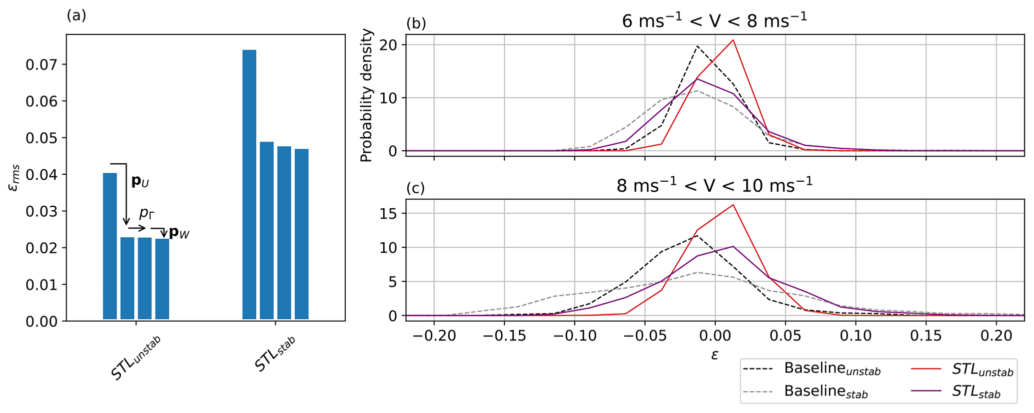
Figure 16 Reduction in the overall error by the activation of different correction types (a). Error probability density distribution for different wind speed ranges (b, c).

An additional problem with the interpretation of the results is due to the fact that the identified flow correction can be affected by the wake combination scheme. As the number of wake overlaps grows towards the trailing edge of the farm, any inaccuracy in the combination model will be amplified there. The results of the figure were obtained with the FLS model, which has been reported to more accurately predict power deep inside the farm (Hamilton et al., 2020). To verify the sensitivity of the solution to this submodel, the identification was repeated with the SOSFS combination, which has been reported to show an improved accuracy in the entrance region where few wakes are present but a less precise power estimation deeper within the farm (Hamilton et al., 2020). With the SOSFS model the correction patterns had similar shapes but a more pronounced magnitude deep in the farm region. Both methods are based on physical arguments and empirical assumptions, and there is no general agreement on whether one is superior to the other. Unfortunately, a correlation check through the STL orthogonal components, as performed in Sect. 3.1.4 for the wake model, is not possible in this case. In fact, these combination models do not have tunable parameters; additionally, tuning the wake models affects all turbines, including the ones with no or limited wake overlaps in the farm entrance region.

These results highlight a problem that deserves attention and further research. In fact, the approach of adding a background correction term to the FLORIS model is somewhat oblivious to the deficiencies of its submodels: for each different wake combination model, a different background flow field is identified that, in the end, is capable of delivering a similar good match of the power predictions with the measurements, compensating possible differences in the behavior of the models. While on the one hand this “obliviousness” is one of the strengths of learning-based data-driven methods, on the other hand it is clearly also one of their main weaknesses because it tends to mask possible problems of the submodels, hindering a full understanding of their true capabilities.

3.2.5 Contributors to the error improvement

Stability affects not only the identified background flow but also the simultaneous tuning of the wake model parameters. For the stable and unstable cases, Table 5 lists the identified wake parameters and compares them to their default values (NREL, 2021). Based on the tuned model parameters, a fully waked turbine at 7 D distance produces 1 % more power in unstable conditions and 7 % in stable conditions when compared to the standard tuning. As previously mentioned, typical values for turbulence intensity were based on the Horns Rev farm because the actual values at the Anholt site were not available. Therefore, these different calibrations could be due to the STL algorithm adjusting the model to the assigned values of ambient turbulence.

Table 5 Results of the wake model tuning, with the initial baseline parameters k_init, the identified values of the additive corrections p_k, and the final tuned parameters k. The last row reports the relative change from k_init to k. The left subcolumn reports values for STL_unstab, whereas the right values reports those for STL_stab.

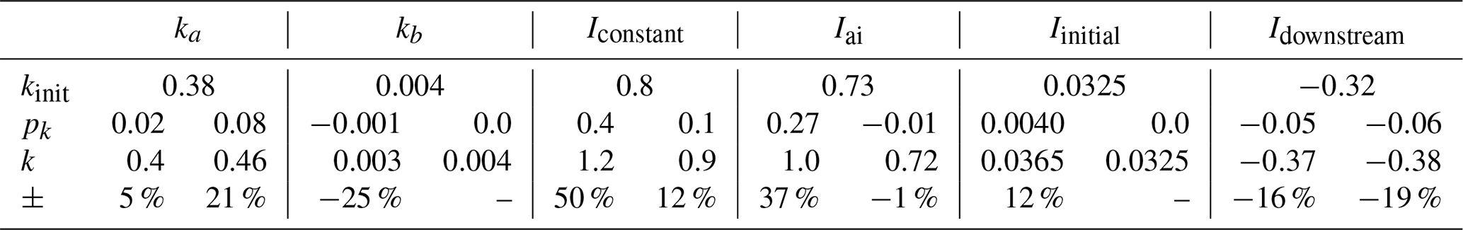
Next, the performance of the STL method was compared to the baseline untuned homogeneous-background case, considering the successive activation of the various correction terms. Figure 16a shows the reduction in the root mean square error defined by Eq. (34), suggesting a few interesting observations.

• The initial error for the baseline model is higher in the stable case than in the unstable one. This is to be expected, since wake and farm effects are more prominent in stable atmospheric conditions.

• The flow correction term produces, similarly to the Sedini case, the largest contribution to the improvement in the error. As for Sedini, even here this term contains clear land-induced effects, generated by the neighboring coastline. However, even more prominent effects are driven by the growth of the boundary layer over the farm because of its relatively large streamwise depth.

• In contrast to the Sedini case, the wind direction correction p_Γ plays only a very minor role here. This is due to the better quality of the yaw signals, which leads to more reliable wind direction estimates that do not suffer from a large bias.

Figure 16b and c show the error probability distributions for the various methods and for two wind speed regimes. Looking at the baseline cases with no parameter tuning, the error has a wide spread, and the flow model is mostly over-predicting wind farm power. Both in the stable and unstable conditions, tuning and learning were able to eliminate over-predictions, reducing the spread and centering the distributions around zero.

4 Conclusions

The present paper has formulated and demonstrated the STL method, which simultaneously calibrates and augments a steady-state parametric wind farm flow model; this work extends an earlier less general formulation first described in Schreiber et al. (2020a). The approach builds on the vast body of knowledge and experience embedded in available engineering wake models. However, it also acknowledges that any such model will always have limited predictive accuracy because of modeling approximations and missing physics. To correct for these deficiencies, a hybrid data-driven strategy is used in the STL approach, where the baseline (white) model is augmented with ad hoc (black-box) extra correction terms. Operational data from the farm are then used to concurrently tune the parameters of the white model and estimate the ones of the black one.

A decomposition of the wind farm flow field by temporal and causal effects forms the basis for the definition of the extra correction terms, together with their functional dependencies and assumed parametric discretizations. The formulation allows for the first time a two-dimensional heterogeneous background flow to be learned directly from operational data. In this sense, the whole wind farm is used as a distributed sensor, which detects the development of the flow within its own boundaries through the response of its wind turbines (which act as local flow sensors). The learned heterogeneous flow is influenced by ambient conditions, terrain orography, roughness, sea state, and plant-induced effects. The learned corrections are not limited to wind speed but can also include heterogeneous wind direction or turbulence intensity fields.

Tuning and learning result in a severely ill-posed identification problem because of the collinearity and/or lack of observability of the redundant unknown parameters. This problem is solved by an SVD-supported MLE. The SVD effectively performs a generalized modal decomposition of the whole solution, which includes the coupled effects of the heterogeneous flow field and of the other tunable model parameters. In this way, combinations of the parameters that are not visible – given the necessarily limited informational content of the available dataset – can be readily discarded, whereas only visible combinations are retained. As a byproduct of this analysis, the examination of the underlying coordinate transformation and resulting mode shapes can be used to reveal interesting features of the solution.

The methodology was showcased via two distinct applications.

For the onshore Sedini farm, the STL revealed the existence of a heterogeneous wind speed field. Augmenting the baseline model with this learned background correction, together with the site-specific tuning of the wake model, resulted in a very significant improvement to the prediction of power output throughout the farm, even when compared to the predictions of the ad hoc tuned baseline model. The learned corrections showed a significant correlation with the terrain elevation, suggesting that the observed heterogeneity of the flow is primarily driven by orographic features of the site. This was further confirmed by over-the-terrain CFD simulations, which also showed a good agreement with the learned corrections. Additionally, the CFD-computed flow field was used as an initial starting guess for the learned correction term; this, however, did not significantly change the results. Furthermore, the STL was able to identify a large bias in the wind direction presumably due to problems with the wind turbine yaw encoders.

For the much larger offshore Anholt farm, the STL revealed the existence of gradients in the inflow, as well as the presence of a strongly direction and stability-dependent highly heterogeneous intra-plant flow field. Comparison with WRF simulations confirmed the origin of the inflow gradients as being caused by the presence of coastlines in close proximity to the farm, as already observed by other authors. The intra-plant flow exhibited clear instances of local accelerations close to the farm edges, suggesting that the flow is “turning” around the obstacle represented by the farm. The observed intra-plant flow appears to be caused by the growth of the boundary layer over the farm. The flow appears to be very significantly influenced by the irregular shape of the farm and by the spacing of the turbines, which would be difficult to capture with simplified analytical models. However, the interpretation of the results was complicated by the effects caused by the interaction of multiple wakes towards the farm trailing edge. It was in fact observed that changes to the wake combination model can affect the identified background flow. Given the present dataset, it was not possible to disentangle the two effects, which remains an open problem that will necessitate further research. Notwithstanding this limitation, the STL was able to very significantly improve the prediction of power when compared to the tuned baseline, no matter what wake combination model was used.

Future work can further improve the STL approach.

On the white-box side of the problem, it would be interesting to add the most recent generation of intra-plant effects. This could help disentangle the causes for the observed heterogeneous background corrections in large farms. Similarly, one should explore more sophisticated wake combination models than the ones used here given their significant effects on the estimated background flow. Models that are parametric (i.e., that can be tuned) would be of particular interest given the “monolithic” parameter estimation performed by the STL.

On the black-box side of the problem, the use of richer datasets than the ones used here could really help illuminate some of the complexities of wind farm flows. For example, operational data accompanied with information on the ambient conditions could help in better discerning the effects of stability on phenomena such as boundary layer growth, blockage, gravity waves, and others. Additionally, extra measurements provided on site by met masts and/or long-range scanning lidars could be fused with the operational data, boosting the informational content of the dataset. Although the grey-box nature of the STL method means that the white-box component can compensate for the lack of information in the data, it is also true that what is not in the white box and not in the data can never be correctly represented by the model. Therefore, future improvements depend to some extent on the richness and quality of the datasets that will be available.

Finally, the STL method should be extended to incorporate unsteady effects by the use of a dynamic version of the baseline engineering wake model. It is envisioned that the steady-state STL could be used, as done here, to adapt the model to represent permanent features of the flow (for example, as caused by a hill), whereas the unsteady STL could be used to render any transient effects (for example, as caused by the finite-speed propagation downstream of set point or inflow changes).

Appendix A: CFD simulations of the flow over the terrain

For the Sedini case, RANS simulations were carried out in OpenFOAM (v2006, 2023) in neutral atmospheric conditions, with the goals of generating a term of comparison for the learned flow corrections (see Sect. 3.1.5) and of providing a non-uniform initial guess to the STL algorithm (Sect. 3.1.6).

The learned corrections ΔU_STL appeared to be independent of the inflow wind speed. In accordance with common practice in industrial applications (van der Laan et al., 2020), the same Reynolds independence was observed for the CFD simulations. The relative variation in wind speed at hub height was computed as

$$\begin{array}{}\text{(A1)}& \mathrm{\Delta }{\widehat{U}}_{\mathrm{CFD}}\left({\mathit{A}}_{\mathrm{0}},Q\right)={\displaystyle \frac{U_{\mathrm{CFD}}-U_{\mathrm{0},\mathrm{CFD}}}{U_{\mathrm{0},\mathrm{CFD}}}}.\end{array}$$

The reference speed U_0,CFD was obtained as the average at the free-stream turbine positions, similarly to the field data case. Due to the Reynolds independence and assumption of neutral conditions, wind direction is the only environmental dependency that was considered, i.e., A₀=Γ₀. One simulation was run for each of the directions ${\mathrm{\Gamma }}_{\mathrm{0}}\in [\mathrm{255},\mathrm{270},\mathrm{285},\mathrm{300}]$^∘.

A1 Domain and mesh generation

A rectangular domain was used because of its simpler mesh generation and clear identification of inlet and outlet compared to other shapes. For each different wind direction case, the terrain was rotated to align the domain with the inflow. Figure A1a shows the domain boundaries and the 2×3 km farm located at its center for the 270^∘ case. The terrain was modeled with satellite DEM data (ASTER, 2021) with a 55 m resolution. A smoothing kernel was applied to the terrain to promote the progressive growth of a boundary layer downstream of the inlet. This was obtained by modifying the terrain elevation (Sørensen et al., 2012) with the following function:

$$\begin{array}{}\text{(A2)}& f_k=\tanh \left[{\left({\displaystyle \frac{r}{R}}\right)}^{\mathrm{6}}\right],\end{array}$$

where R=6 km is the radius where the terrain elevation vanishes, obtaining the smoothed out domain shown in Fig. A1b. A domain height of only 3 km was found to be sufficient to ensure an undisturbed flow at the top of the domain, although this value is smaller than the one recommended by Sørensen et al. (2012).

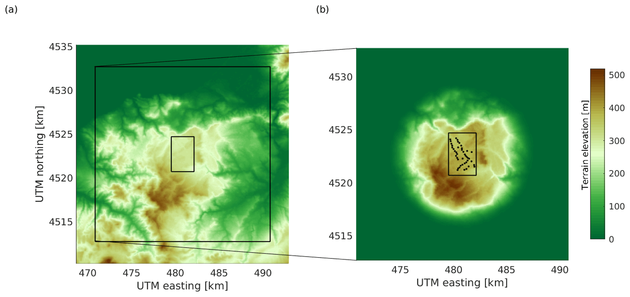
Figure A1 Terrain elevation around the Sedini wind farm (a). The large rectangle shows the CFD domain, whereas the small one shows the perimeter of the wind farm (visible in b). Terrain elevation after application of the smoothing kernel (b). The panels correspond to the 270^∘ wind direction case; for other directions, the computational domain was rotated accordingly.

A regular background mesh was generated with the blockMesh tool that is part of the OpenFOAM distribution. In the horizontal direction, $N_x=N_y=\mathrm{500}$ cells were used, resulting in a resolution of $\mathrm{\Delta }x=\mathrm{\Delta }y=\mathrm{40}$ m. In the vertical direction, the domain was divided in two parts at a height of 1 km. The top section had a constant vertical spacing of Δz_top=100 m. In the bottom section, a grading scheme was used to progressively increase the spacing from Δz_bott=5 m close to the ground to 25 m at the split section. An additional layer with a thickness of 2.7 m was added to further refine the region close to the ground, resulting in an average aspect ratio of the wall-adjacent cells equal to 14.8. Finally, the tool SnappyHexMesh was used to adapt the $\approx \mathrm{16.5}\times {\mathrm{10}}^{\mathrm{6}}$ cell grid to the terrain contour.

A2 Boundary conditions and numerical setup

As simulations were performed only for neutral conditions, buoyancy effects were not included. Furthermore, Coriolis effects were also neglected as only the velocity at hub height is of interest, which is very close to the surface. The k-ϵ model was used for turbulent stresses. As suggested by Richards and Hoxey (1993), the model constant σ_ϵ was set to the value of 1.11, which is typical of atmospheric flows, while the other model parameters were left at their default values (Launder and Spalding, 1974).

The domain boundary conditions were imposed as follows. A logarithmic velocity profile was imposed at the inlet, with a roughness length of z₀=0.01 – corresponding to open terrain, as the site has not much vegetation – and a hub-height speed of U_hh=8 m s⁻¹. The inlet profiles for turbulent kinetic energy k_turb, eddy viscosity ν_T, and dissipation of turbulent kinetic energy ϵ_turb were implemented with the ABL boundary conditions of OpenFOAM version v2006 (Release Notes v2006, 2020), based on Hargreaves and Wright (2007) and Yang et al. (2009). No-slip conditions and wall functions based on Hargreaves and Wright (2007) were used in proximity to the terrain. At the top of the domain, a constant shear stress was used to drive the flow, while symmetry conditions were applied to the side walls. At the outlet, the kinematic pressure was set to zero, while zero gradient conditions were imposed for all other variables.

A second-order accurate linear discretization scheme was used for the divergence terms. The problem was solved with simpleFoam, an implementation of the SIMPLE algorithm. The setup was first tested in an empty domain, where it was able to establish an equilibrium ABL with constant velocity profile from inlet to outlet. Simulations were run with 322 cores and converged after ca. 1200 iterations.

A3 Grid convergence

To investigate grid convergence, the mesh was progressively coarsened in both the horizontal and vertical directions (in the latter case, only in the bottom section of the domain), obtaining 10 %, 30 %, and 50 % fewer grid points, respectively. Table A1 lists the defining parameters for the fine and the coarser domains for the 270^∘ direction; similar results were obtained for the other directions. The average cell height in the bottom section of the domain is denoted 〈Δz_bott〉.

Figure A2 shows the average hub-height speed difference 〈ϵ_GL,i〉 for the three coarser cases with respect to the fine-grid solution, where ${\mathit{ϵ}}_{\mathrm{GL},i}=(U_{\mathrm{GL},\mathrm{base}}-U_{\mathrm{GL},i})/U_{\mathrm{GL},\mathrm{base}}$. The coarser solution, based on 50 % fewer grid points than the fine one, differs only by about 4 %. The curve trend indicates that the fine-grid solution can be considered to be at convergence.

Table A1 Mesh characteristics for the grid convergence study for the 270^∘ direction.

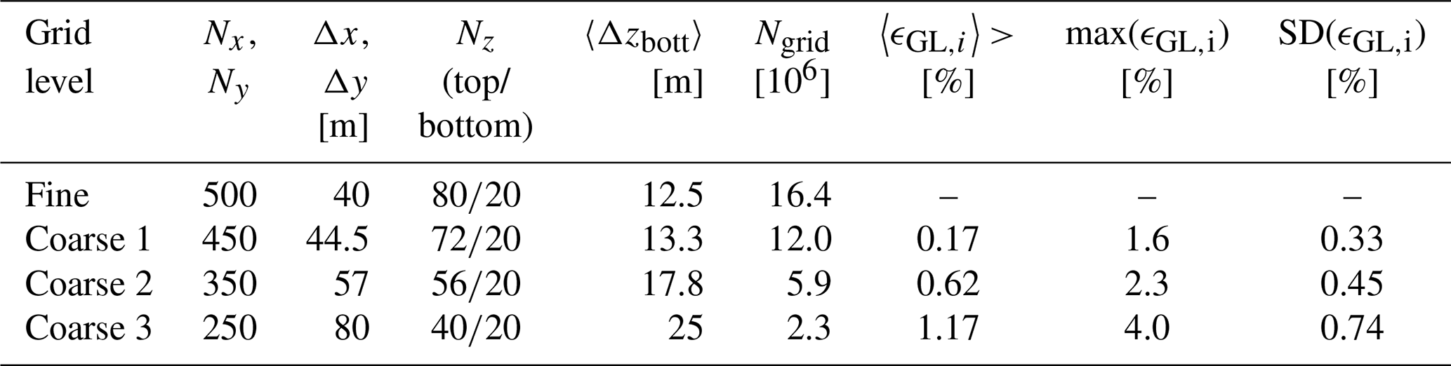
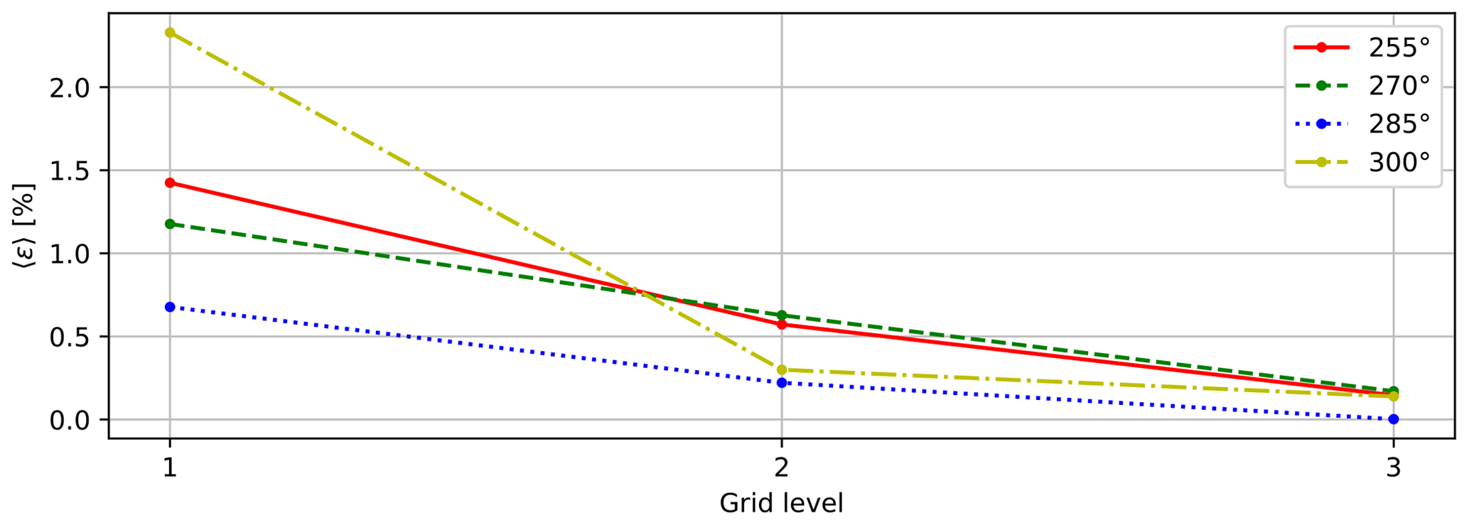
Figure A2 Average relative difference in hub-height speed for grids of increasing coarseness.

Appendix B: Results for the Sedini wind plant during day and nighttime operation

Figure B1 Normalized measured and calculated power for all turbines for all 5^∘ bins in the investigated 245–310^∘ sector for wind speeds in the range of 6–8 m s⁻¹ during daytime operation. Bins with <10 observations are not shown. The uncertainty band indicates the standard deviation in the bins. Δh is the foundation elevation difference with respect to the farm average, and it is indicated by the color of the frame of each subplot.

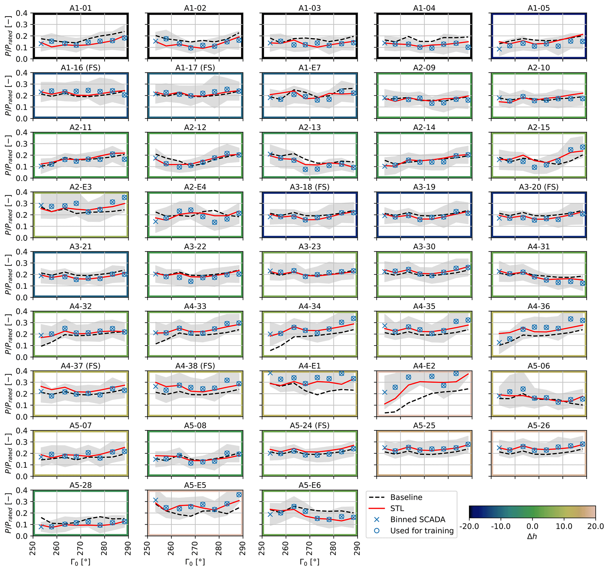
Figure B2 Normalized measured and calculated power for all 5^∘ bins in the investigated 245–310^∘ sector for wind speeds in the range of 6–8 ms ⁻¹ during nighttime operation.

Appendix C: Nomenclature

A	Vector of ambient state variables
E	Fisher matrix
F	Flow quantity
h	Elevation
I	Turbulence intensity
J	Cost function
k	Wake model parameter
L	Obukhov length
M	Sensitivity matrix
n	Shape function vector
N	Number of observations
Nt	Number of turbines
Np	Number of STL parameters
NID	Number of retained (i.e., identified)
	orthogonal parameters
p	Complete vector of free STL correction
	parameters
pF	Correction node values to model flow
	heterogeneity
pW	Correction parameters for wake model
	tuning
P	Turbine power
P	Inverse of the Fisher matrix
Q	Spatial position
r	Residual between measurement and model
	output
R	Measurement covariance matrix
s	Singular value
S	Matrix of singular values
U	Wind speed at hub height
U	Matrix of left singular vectors
v	Right singular vector
V	Matrix of right singular vectors
w	Measurement weight
y	Model output
z	Measurement
z0	Roughness length
Γ	Wind direction
ΔF	Heterogeneous flow quantity correction
ϵ	Error
θ	Orthogonal parameter
ρ	Density
ϱ	Correlation coefficient
σm	Measurement variance
σt	Observability threshold
Ψ	Matrix of eigenshapes
$\overline{(.)}$	Constant-in-time component
$\stackrel{\mathrm{̃}}{(.)}$	Slow component
$(.{)}^{\prime }$	Turbulent (fast) component
(.)0	Site-average quantity
$\widehat{(.)}$	Scaled quantity
〈.〉	Average operator
ABL	Atmospheric boundary layer

FLORIS	FLOw Redirection and Induction in
	Steady State
FLS	Freestream linear superposition
Lidar	Light detection and ranging
MLE	Maximum likelihood estimation
RANS	Reynolds-averaged Navier–Stokes
REWS	Rotor-equivalent wind speed
SCADA	Supervisory control and data acquisition
SOSFS	Sum of squared freestream superposition
STL	Simultaneous tuning and learning
SVD	Singular value decomposition
TI	Turbulence intensity
WRF	Weather Research and Forecasting model