Vortex model of the aerodynamic wake of airborne wind energy systems

Understanding and modeling the aerodynamic wake of airborne wind energy systems (AWESs) is crucial for estimating the performance and defining the design of such systems, as tight trajectories increase induced velocities and thus decrease the available power, while unnecessarily large trajectories increase power losses due to the gravitational potential energy exchange. The aerodynamic wake of crosswind AWESs flying circular trajectories is studied here with vortex methods. The velocities induced at the AWES from a generic helicoidal vortex filament, trailed by a position on the AWES wing, are modeled with an expression for the near vortex filament and one for the far vortex filament. The near vortex filament is modeled as the first half rotation of the helicoidal filament, with its axial component being neglected. The induced drag due to the near wake, built up from near vortex filaments, is found to be similar to the induced drag the AWES would have in forward flight. The far wake is modeled as two semi-infinite vortex ring cascades with opposite intensity. An approximate solution for the axial induced velocity at the AWES is given as a function of the radial (known) and axial (unknown) position of the vortex rings. An explicit and an implicit closure model are introduced to link the axial position of the vortex rings with the other quantities of the model. The aerodynamic model, using the implicit closure model for the far wake, is validated with the lifting-line free-vortex wake method implemented in QBlade. The model is suitable to be used in time-marching aero-servo-elastic simulations and in design and optimization studies.

1 Introduction

Airborne wind energy (AWE) refers to the field of wind energy in which tethered airborne systems are used to harvest wind power at high altitudes. Airborne wind energy systems (AWESs) are typically classified based on their flight operations, which can be crosswind, tether-aligned and rotational as described by Vermillion et al. (2021). Electric power is generated with onboard wind turbines and transferred to the ground through the tether (Fly-Gen) or generated directly on the ground by a moving or fixed ground station (Ground-Gen). This work focuses on crosswind AWESs, and the results are applicable to both Ground-Gen and Fly-Gen systems which are characterized by a single wing.

Loyd (1980) first derived the power equation for crosswind AWESs, based on given lift and drag coefficients of the AWES. To properly evaluate system performance, special care should be given to the estimation of the drag coefficient, as it includes contributions from the tether drag (see Trevisi et al., 2020a, for more details) and from the induced drag. The latter is the result of the induced velocities generated by the lifting surface and its wake on the lifting surface itself. For wind-harvesting devices, the induced velocities effectively reduce the incoming wind and thus the available power. Generating high aerodynamic lift could be counterproductive for power generation, as induced velocities grow consequently. For flying wings, the induced velocities effectively rotate the inflow field of an induced angle. As lift is, by its definition, perpendicular to the local velocity, it is rotated by this induced angle, generating an aerodynamic force component parallel to the motion, namely the induced drag. High aerodynamic lift then generates high induced drag, which needs to be compensated by the propulsive thrust.

As AWESs are wind-harvesting devices, the evaluation of the induced velocity is of extreme importance to properly estimate the power production. The effect of the induced velocity can be taken into account by reducing the incoming wind, as typically done for wind turbines, or by including them in the induced drag estimation, as typically done for flying wings.

Learning from conventional wind energy, the induced velocities for AWE are estimated in the literature with momentum-based and vortex-based methods. High-fidelity computational fluid dynamics (CFD) methods are typically used to study the wake characteristics and validate lower-fidelity models.

Initially, the applicability of momentum methods for AWE was doubted (Loyd, 1980; Archer, 2013; Costello et al., 2015), as the definition of swept area is not settled but by intuition way larger than the AWES wing. Recently, however, momentum methods have been developed for AWE, with De Lellis et al. (2018) and Kheiri et al. (2018, 2019) independently generalizing momentum theory to compute the induced velocity. This is derived by equating the aerodynamic lift of the AWES with the thrust applied to the annulus swept by the wing, with the momentum formulation. The power equations for Fly-Gen and Ground-Gen AWESs are then derived by reducing the incoming wind of the induced velocities. They find that Fly-Gen AWESs have higher power generation potential compared to Ground-Gen. Akberali et al. (2021) extend the derivation for AWESs with an elevation and a side-slip angle. Kaufman-Martin et al. (2021), Kheiri et al. (2022) and Karakouzian et al. (2022) study, with the aim of understanding the interaction of AWESs in a wind farm, the downstream AWES wake shape and characteristics with momentum and mass conservation considerations, finding a good agreement with CFD results.

Gaunaa et al. (2020) point out that using momentum theory to evaluate the induction of an AWES, which is described by 3D polars, is not physically consistent. Momentum theory is indeed used in wind turbine aerodynamics to compute the local velocity triangle of the airfoil (2D polars) in the wind turbine blade. If the AWES is described by 3D polars (i.e., the drag coefficient includes the induced drag coefficient that the AWES would have in a forward flight) in the momentum formulation, then a part of the wake would be counted twice. If, instead, momentum theory is used to evaluate the velocity triangle of an airfoil (2D polars) in the AWES wing, then root and tip corrections would be needed to take into account that the rotor is not a disc built up of an infinite number of wings but one single wing. The root and tip corrections for AWESs would however differ largely from conventional wind turbines corrections, as these are developed for blades extending almost to the rotation axis and need to be reworked. Gaunaa et al. (2020) then build a vortex-based engineering model, which is physically consistent, and it is tuned with CFD simulations. Another vortex method, based on the vortex tube model, is developed by Leuthold et al. (2019) for an AWE system composed of more wings flying in the same annulus to compute the induction at the AWESs mid-span. This model takes as inputs the system thrust coefficient, relative radius and reel-out factor.

As the field counts a limited number of prototypes with a limited number of flying hours, the benchmark of engineering models is typically done with higher-fidelity codes, instead of experiments. For aerodynamic models, CFD studies then represent the reference. Haas and Meyers (2017) describe the wake characteristics for a given aircraft in a Fly-Gen and Ground-Gen circular path with a large-eddy simulation (LES) setup. Aerodynamic forces, applied with an actuator line technique, are computed to impose an induction of $\mathrm{1}/\mathrm{3}$ at the kite location. Haas et al. (2019) further develop the same LES framework by including an optimal control problem for Ground-Gen AWESs in non-turbulent and turbulent sheared inflow conditions. Mehr et al. (2020) investigate the aerodynamic interaction of the onboard wind turbines with the main wing in a crosswind circular maneuver with a viscous vortex particle method. The main wing wake is however removed one span downstream from the trailing edge, not resolving the helicoidal wake. Branlard et al. (2022) extend the AeroDyn module of OpenFAST through the open-source lifting-line vortex code OLAF to support arbitrary collections of wings, rotors and towers. Complex geometries, such as AWESs, can then be handled by OLAF.

The present work builds on the considerations from Gaunaa et al. (2020) to develop a vortex-based engineering model, which is physically consistent. The use of vortex methods, described by Branlard (2017), allows for modeling the induction at the AWES due to its own wake. The goal of this work is to analytically study the wake produced by AWESs flying circular trajectories by modeling how geometrical and aerodynamic quantities influence the induced velocities. This model can be used to find how the induced velocities vary along the wing span and to refine the power equations.

An analytical model of the helicoidal wake will inform about the validity bounds of the assumption of a straight wake employed in the engineering models (Bauer et al., 2018; Trevisi et al., 2020b, among others) and in computational studies focusing on the aerodynamic characterization of the AWES (Viré et al., 2020; Castro-Fernández et al., 2021, among others).

Modeling the induced velocities along the wing span will instead improve the engineering aerodynamic models for load estimation (Damiani et al., 2019) and the flight dynamic models (Trevisi et al., 2021a).

A refined power equation, including the contribution from the helicoidal wake, will inform the designer in an intuitive way about the effects of changing geometrical and aerodynamic quantities on the overall performance. This could be used in low-fidelity system design and optimization studies (Bauer et al., 2018; Trevisi et al., 2021b, among others). The power equation refinement will be performed in an upcoming work to limit this paper's scope and length.

This paper is organized as follows: in Sect. 2, the modeling of the induction produced by a helicoidal vortex filament is introduced. The helicoidal vortex filament can be described as a near vortex filament, modeled by a half revolution of the filament in the rotor plane, and a far vortex filament, modeled by an infinite series of vortex rings. In Sect. 3, the near-wake model and the relative induced drag coefficient are derived. In Sect. 4, the far-wake model, which depends on the radial (known) and axial (unknown) position of the vortex rings, is derived. An explicit and an implicit model are proposed to find the axial position. In Sect. 5, the model is validated with QBlade, which uses a lifting-line free-vortex wake method. In Sect. 6, the main conclusions are discussed.

2 Modeling of a helicoidal vortex filament

In this section, the modeling framework of the induced velocities produced by a non-expanding helicoidal vortex filament is introduced. As the induced velocities at a given point are found by integrating the contributions of the vortex filaments composing the aerodynamic wake, they are first studied in this section. The formulation introduced in this section will be used to derive a near- and a far-wake model in the next sections.

AWESs flying crosswind typically follow a circular or a figure-of-eight pattern. The present work analyzes the wake produced by circular trajectories, which are contained in a plane perpendicular to the incoming wind, as in Fig. 1. It is here assumed that the AWES has a constant rotational speed, and its wings are on the rotational plane. This condition is also considered by the other studies concerning AWES wakes (e.g., De Lellis et al., 2018; Kheiri et al., 2018; Gaunaa et al., 2020; Kaufman-Martin et al., 2021). Moreover, Trevisi et al. (2022a) show that these are the optimal trajectories for a Fly-Gen maximizing thrust power with constant inflow. Optimal trajectories for a Fly-Gen maximizing electric power including wind shear can be understood as a perturbation of this solution. Additionally, one can study the flight mechanics of the AWES for this condition (Trevisi et al., 2021a).

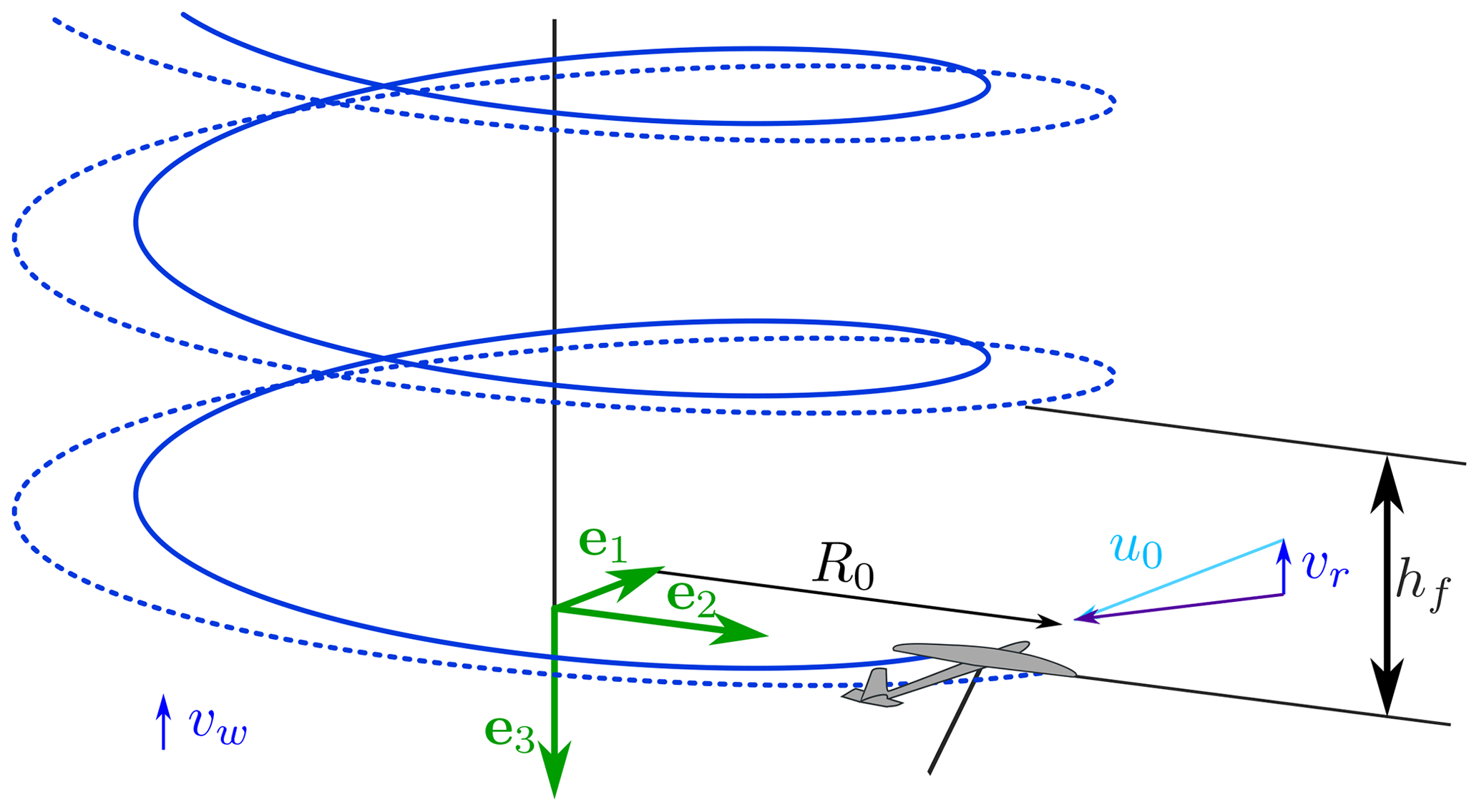
Figure 1 Wake structure of an AWES flying circular trajectories. The solid and dashed lines represent the left and right rolled-up vortices respectively.

Referring to Fig. 1, the AWES moves along a circular trajectory in the plane (e₁,e₂) with radius R₀. The versor e₃ points upwind, and therefore the wind velocity is ${\mathit{v}}_{\mathrm{w}}=-v_{\mathrm{w}}{\mathit{e}}_{\mathrm{3}}$. For Ground-Gen AWESs, the relative wind velocity at the AWES is ${\mathit{v}}_{\mathrm{r}}={\mathit{v}}_{\mathrm{w}}-{\mathit{v}}_{\mathrm{o}}$, where ${\mathit{v}}_{\mathrm{o}}=-v_{\mathrm{o}}{\mathit{e}}_{\mathrm{3}}$ is the reel-out velocity of the tether, assumed to be only along the axial direction. For Fly-Gen AWESs, the relative wind velocity at the AWES coincides with the wind speed v_r=v_w, as the tether is fixed at the ground station. The vortices trailed by the AWES are transported downwind by the wind and have a helicoidal shape. Following the assumptions of Prandtl and Goldstein in the derivation of the tip-loss correction for wind turbines, no distortion and no expansion of the wake are assumed (Branlard, 2017).

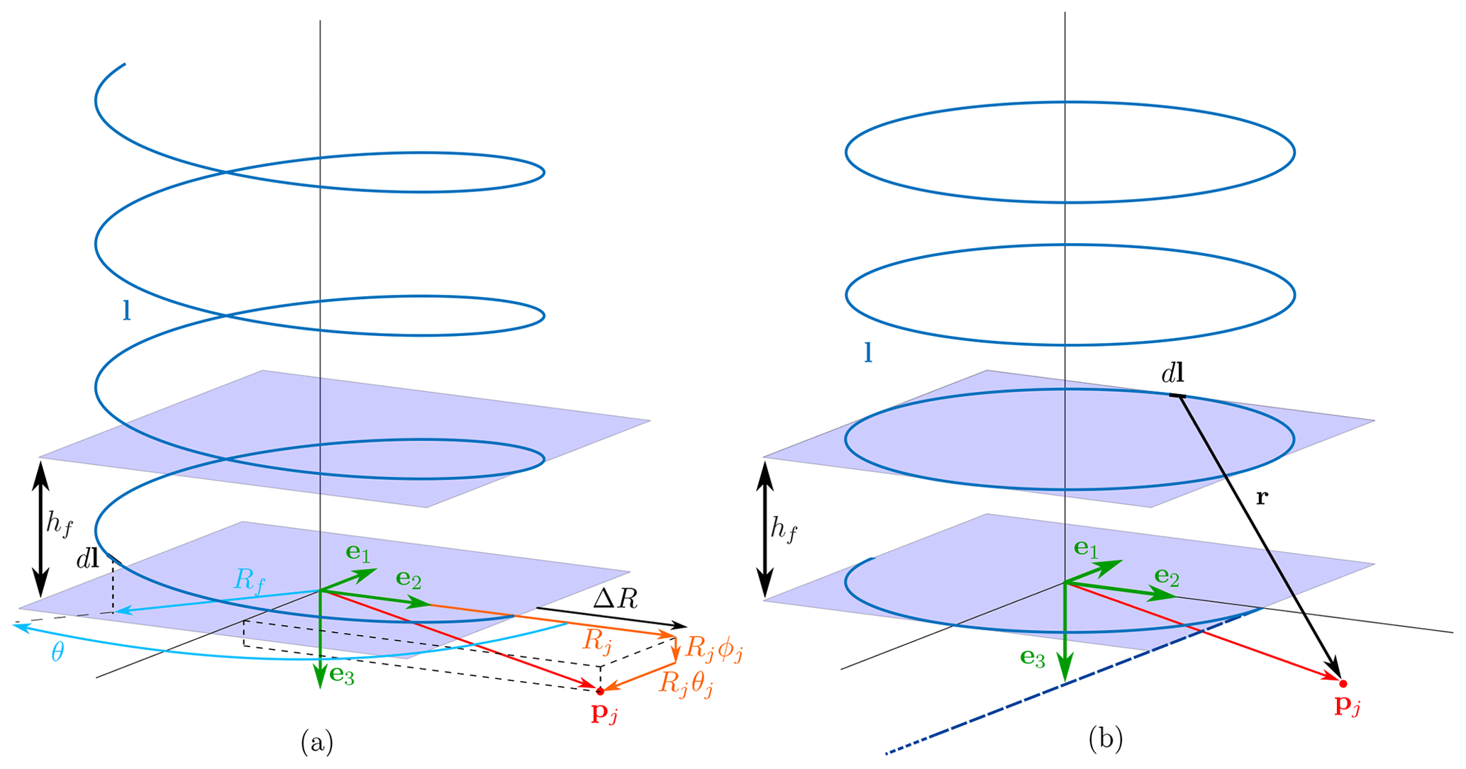
The geometry of the helicoidal vortex filament is shown in Fig. 2a. The radius of the filament is R_f, and the pitch is h_f. The induction is evaluated at a generic point p_j, with radius R_j. With these definitions, the radial difference ΔR between the evaluation point and the filament is

$$\begin{array}{}\text{(1)}& \mathrm{\Delta }R=R_j-R_{\mathrm{f}},\end{array}$$

and it is normalized with the evaluation radius as

$$\begin{array}{}\text{(2)}& \mathit{\eta }={\displaystyle \frac{\mathrm{\Delta }R}{R_j}}=\mathrm{1}-{\displaystyle \frac{R_{\mathrm{f}}}{R_j}}.\end{array}$$

Note that η=0 when ΔR=0, η=1 when $R_j\to +\mathrm{\infty }$ and $\mathit{\eta }\to -\mathrm{\infty }$ when R_j→0. The normalized position of the vortex filament with respect to the mid-span turning radius R₀ (see Fig. 1) is indicated as

$$\begin{array}{}\text{(3)}& {\mathit{\eta }}_{\mathrm{0}}={\displaystyle \frac{R_{\mathrm{0}}-R_{\mathrm{f}}}{R_{\mathrm{0}}}}=-{\displaystyle \frac{y_{\mathrm{f}}}{R_{\mathrm{0}}}},\end{array}$$

where y_f indicates the position of the vortex filament along the wing span direction. The filament radius R_f can then be expressed as

$$\begin{array}{}\text{(4)}& R_{\mathrm{f}}=R_j(\mathrm{1}-\mathit{\eta })=R_{\mathrm{0}}\left(\mathrm{1}-{\mathit{\eta }}_{\mathrm{0}}\right).\end{array}$$

Figure 2 (a) Helicoidal vortex filament and (b) relative modeling after assumptions.

The helix can be modeled as

$$\begin{array}{}\text{(5)}& \mathit{l}=\left[\begin{array}{l}-R_{\mathrm{f}}\sin \left(\mathit{\theta }\right)\\ R_{\mathrm{f}}\cos \left(\mathit{\theta }\right)\\ -\frac{h_f}{\mathrm{2}\mathit{\pi }}\mathit{\theta }\end{array}\right]=R_j(\mathrm{1}-\mathit{\eta })\left[\begin{array}{l}-\sin \left(\mathit{\theta }\right)\\ \cos \left(\mathit{\theta }\right)\\ -\frac{\mathrm{1}}{\mathrm{1}-{\mathit{\eta }}_{\mathrm{0}}}\frac{\mathit{\theta }}{{\mathit{\lambda }}_{\mathrm{0}}}\end{array}\right],\end{array}$$

where $\frac{R_{\mathrm{0}}}{R_j}=\frac{\mathrm{1}-\mathit{\eta }}{\mathrm{1}-{\mathit{\eta }}_{\mathrm{0}}}$ (Eq. 4), $\mathit{\theta }\in [\mathrm{0},\mathrm{\infty }[$ is the angular parameter of the helix and it is assumed that the helix pitch of any vortex filament h_f trailed by the wing is equal to the helix pitch h₀ of the vortex filament at the wing center. The normalized torsional parameter λ₀ (Branlard, 2017) is the ratio between the projected circumference length 2πR₀ and the helix pitch h₀ of the vortex filament:

$$\begin{array}{}\text{(6)}& {\mathit{\lambda }}_{\mathrm{0}}={\displaystyle \frac{\mathrm{2}\mathit{\pi }{R}_{\mathrm{0}}}{h_{\mathrm{0}}}}.\end{array}$$

The induced velocities w_j,f produced by the filament of vorticity Γ at a point p_j is found using the Biot–Savart law:

$$\begin{array}{}\text{(7)}& {\mathit{w}}_{j,\mathrm{f}}={\displaystyle \frac{\mathrm{\Gamma }}{\mathrm{4}\mathit{\pi }}}\underset{\mathrm{0}}{\overset{+\mathrm{\infty }}{\int }}{\displaystyle \frac{d\mathit{l}\times \mathit{r}}{|\mathit{r}{|}^{\mathrm{3}}}},\end{array}$$

where

$$\begin{array}{}\text{(8)}& d\mathit{l}=-R_j(\mathrm{1}-\mathit{\eta })\left[\begin{array}{l}\cos \left(\mathit{\theta }\right)\\ \sin \left(\mathit{\theta }\right)\\ \frac{\mathrm{1}}{\left(\mathrm{1}-{\mathit{\eta }}_{\mathrm{0}}\right){\mathit{\lambda }}_{\mathrm{0}}}\end{array}\right]d\mathit{\theta }\end{array}$$

and $\mathit{r}={\mathit{p}}_j-\mathit{l}$. As the vortex filaments are trailed by the wing and the evaluation point is typically on the aircraft itself, p_j is modeled as

$$\begin{array}{}\text{(9)}& {\mathit{p}}_j=\left[\begin{array}{l}-R_j{\mathit{\theta }}_j\\ R_j\\ R_j{\mathit{\varphi }}_j\end{array}\right],\end{array}$$

where θ_j and ϕ_j define the 3D position of the evaluation point and are assumed to be small (see Fig. 2a). r can then be expressed as

$$\begin{array}{}\text{(10)}& \begin{array}{rl}\mathit{r}& =R_j\left[\begin{array}{l}-{\mathit{\theta }}_j\\ \mathrm{1}\\ {\mathit{\varphi }}_j\end{array}\right]-R_j(\mathrm{1}-\mathit{\eta })\left[\begin{array}{l}-\sin \left(\mathit{\theta }\right)\\ \cos \left(\mathit{\theta }\right)\\ -\frac{\mathit{\theta }}{\left(\mathrm{1}-{\mathit{\eta }}_{\mathrm{0}}\right){\mathit{\lambda }}_{\mathrm{0}}}\end{array}\right]\\ & =-R_j\left[\begin{array}{l}{\mathit{\theta }}_j-(\mathrm{1}-\mathit{\eta })\sin \left(\mathit{\theta }\right)\\ (\mathrm{1}-\mathit{\eta })\cos \left(\mathit{\theta }\right)-\mathrm{1}\\ -{\mathit{\varphi }}_j-\frac{\mathrm{1}-\mathit{\eta }}{\mathrm{1}-{\mathit{\eta }}_{\mathrm{0}}}\frac{\mathit{\theta }}{{\mathit{\lambda }}_{\mathrm{0}}}\end{array}\right].\end{array}\end{array}$$

When looking for the axial induced velocity $w_{j,\mathrm{f}}={\mathit{w}}_{j,f}\cdot {\mathit{e}}_{\mathrm{3}}$, the third component of the numerator of Eq. (7) becomes

$$\begin{array}{}\text{(11)}& (d\mathit{l}\times \mathit{r})\cdot {\mathit{e}}_{\mathrm{3}}=-{\displaystyle \frac{R_j^{\mathrm{2}}}{\mathit{\eta }}}\underset{N_{\sim }}{\underbrace{\mathit{\eta }(\mathrm{1}-\mathit{\eta })\left(\cos (\mathit{\theta }-{\mathit{\theta }}_j)-(\mathrm{1}-\mathit{\eta })\right)}}d\mathit{\theta },\end{array}$$

where the subscript ∼ indicates a periodicity in θ.

The norm of r squared, removing the second-order terms in θ_j and ϕ_j and using the trigonometric relation $\cos (\mathit{\theta }-{\mathit{\theta }}_j)\approx \cos \left(\mathit{\theta }\right)+\sin \left(\mathit{\theta }\right){\mathit{\theta }}_j$, can be expressed as

$$\begin{array}{}\text{(12)}& \begin{array}{rl}|\mathit{r}{|}^{\mathrm{2}}& \approx R_j^{\mathrm{2}}\left[\underset{D_{\sim }}{\underbrace{\mathrm{1}-\mathrm{2}(\mathrm{1}-\mathit{\eta })\cos \left(\mathit{\theta }-{\mathit{\theta }}_j\right)+(\mathrm{1}-\mathit{\eta }{)}^{\mathrm{2}}}}\right.\\ & \left.+\underset{D_{/}}{\underbrace{\mathrm{2}{\mathit{\varphi }}_j\left({\displaystyle \frac{\mathrm{1}-\mathit{\eta }}{\mathrm{1}-{\mathit{\eta }}_{\mathrm{0}}}}{\displaystyle \frac{\mathit{\theta }}{{\mathit{\lambda }}_{\mathrm{0}}}}\right)+{\left({\displaystyle \frac{\mathrm{1}-\mathit{\eta }}{\mathrm{1}-{\mathit{\eta }}_{\mathrm{0}}}}{\displaystyle \frac{\mathit{\theta }}{{\mathit{\lambda }}_{\mathrm{0}}}}\right)}^{\mathrm{2}}}}\right],\end{array}\end{array}$$

where a distinction between the periodic D_∼ and the non-periodic part $D_{/}$ is made.

Finally, the Biot–Savart law (Eq. 7) can be written considering Eqs. (11) and (12) as

$$\begin{array}{}\text{(13)}& \begin{array}{rl}{w}_{j,\mathrm{f}}& =-{\displaystyle \frac{\mathrm{\Gamma }}{\mathrm{4}\mathit{\pi }\mathrm{\Delta }R}}\\ & \underset{\mathrm{0}}{\overset{+\mathrm{\infty }}{\int }}{\displaystyle \frac{N_{\sim }\left(\mathit{\eta },\left(\mathit{\theta }-{\mathit{\theta }}_j\right)\right)}{{\left(D_{\sim }\left(\mathit{\eta },\left(\mathit{\theta }-{\mathit{\theta }}_j\right)\right)+D_{/}\left({\mathit{\varphi }}_j,\left(\frac{\mathrm{1}-\mathit{\eta }}{\mathrm{1}-{\mathit{\eta }}_{\mathrm{0}}}\frac{\mathit{\theta }}{{\mathit{\lambda }}_{\mathrm{0}}}\right)\right)\right)}^{\frac{\mathrm{3}}{\mathrm{2}}}}}d\mathit{\theta }\\ & =-{\displaystyle \frac{\mathrm{\Gamma }}{\mathrm{4}\mathit{\pi }\mathrm{\Delta }R}}\mathrm{{\rm Y}},\end{array}\end{array}$$

where the term outside the integral models the induced velocity produced by a semi-infinite straight vortex filament pointing in the −e₁ direction (Fig. 2b) on the point ${\mathit{p}}_j({\mathit{\theta }}_j=\mathrm{0},{\mathit{\varphi }}_j=\mathrm{0})$ (Eq. 9). The integral, denoted with Υ, can be understood as a shape factor multiplying it.

By splitting the integration interval as $[\mathrm{0},+\mathrm{\infty }[=[\mathrm{0},\mathit{\pi }]\cup [\mathit{\pi },\mathrm{3}\mathit{\pi }]\cup [\mathrm{3}\mathit{\pi },\mathrm{5}\mathit{\pi }]\cup \mathrm{\dots }=[\mathrm{0},\mathit{\pi }]\cup {\bigcup }_{k=\mathrm{1}}^{\mathrm{\infty }}(\mathrm{2}\mathit{\pi }k+[-\mathit{\pi },+\mathit{\pi }\left]\right)$, the integral can be rewritten as an infinite summation of integrals. By properly rewriting the non-periodic terms, Eq. (13) becomes

$$\begin{array}{}\text{(14)}& \begin{array}{rl}{w}_{j,\mathrm{f}}& =-{\displaystyle \frac{\mathrm{\Gamma }}{\mathrm{4}\mathit{\pi }\mathrm{\Delta }R}}\\ & \left[\stackrel{{\mathrm{{\rm Y}}}^{\mathrm{n}}:\mathrm{near}\mathrm{vortex}\mathrm{filament}}{\overbrace{\underset{\mathrm{0}}{\overset{\mathit{\pi }}{\int }}{\displaystyle \frac{N_{\sim }\left(\mathit{\eta },\left(\mathit{\theta }-{\mathit{\theta }}_j\right)\right)}{{\left(D_{\sim }\left(\mathit{\eta },\left(\mathit{\theta }-{\mathit{\theta }}_j\right)\right)+D_{/}\left({\mathit{\varphi }}_j,\left(\frac{\mathrm{1}-\mathit{\eta }}{\mathrm{1}-{\mathit{\eta }}_{\mathrm{0}}}\frac{\mathit{\theta }}{{\mathit{\lambda }}_{\mathrm{0}}}\right)\right)\right)}^{\frac{\mathrm{3}}{\mathrm{2}}}}}d\mathit{\theta }}}\right.\\ & \left.+\underset{\mathrm{far}\mathrm{vortex}\mathrm{filament}}{\underbrace{\sum _{k=\mathrm{1}}^{\mathrm{\infty }}\underset{-\mathit{\pi }}{\overset{\mathit{\pi }}{\int }}{\displaystyle \frac{N_{\sim }\left(\mathit{\eta },\left(\mathit{\theta }-{\mathit{\theta }}_j\right)\right)}{{\left(D_{\sim }\left(\mathit{\eta },\left(\mathit{\theta }-{\mathit{\theta }}_j\right)\right)+D_{/}\left({\mathit{\varphi }}_j,\left(\frac{\mathrm{1}-\mathit{\eta }}{\mathrm{1}-{\mathit{\eta }}_{\mathrm{0}}}\frac{(\mathrm{2}\mathit{\pi }k+\mathit{\theta })}{{\mathit{\lambda }}_{\mathrm{0}}}\right)\right)\right)}^{\frac{\mathrm{3}}{\mathrm{2}}}}}d\mathit{\theta }}}\right].\end{array}\end{array}$$

In Eq. (14) a distinction between near and far vortex filament is made, noting that the near vortex filament (i.e., the first integral) models the induction produced by the first half revolution of the filament, whereas the far vortex is modeled through the infinite summation of integrals.

The integrals modeling the near and the far vortex filament have terms proportional to θ in the denominator. These terms physically represent the contribution to $\left|\mathit{r}\right|$ from the projection of r along e₃, and they have a maximum value at $\mathit{\theta }=\pm \mathit{\pi }$, which is also where the projection of r in the (e₁,e₂) plane is largest. This suggests that the overall contribution of the terms proportional to θ to the integral should be limited.

By neglecting the terms proportional to θ, the model of the helicoidal vortex filament in Fig. 2a reduces into the model of Fig. 2b (i.e., half a vortex ring plus a semi-infinite vortex ring cascade). Note that, with the split of the integration interval introduced in Eq. (14), the axial distance of the vortex rings corresponds to the helix pitch and the integration bounds of the far-wake integrals are symmetric.

The axial velocity at point p_j, induced by the idealized helicoidal vortex filament, is then approximated as

$$\begin{array}{}\text{(15)}& \begin{array}{rl}{w}_{j,\mathrm{f}}& \approx -{\displaystyle \frac{\mathrm{\Gamma }}{\mathrm{4}\mathit{\pi }\mathrm{\Delta }R}}\left[\underset{{\mathrm{{\rm Y}}}^{\mathrm{n}}}{\underbrace{\underset{\mathrm{0}}{\overset{\mathit{\pi }}{\int }}{\displaystyle \frac{N_{\sim }\left(\mathit{\eta },\left(\mathit{\theta }-{\mathit{\theta }}_j\right)\right)}{D_{\sim }{\left(\mathit{\eta },\left(\mathit{\theta }-{\mathit{\theta }}_j\right)\right)}^{\frac{\mathrm{3}}{\mathrm{2}}}}}d\mathit{\theta }}}+\sum _{k=\mathrm{1}}^{\mathrm{\infty }}\underset{-\mathit{\pi }}{\overset{\mathit{\pi }}{\int }}\right.\\ & \left.{\displaystyle \frac{N_{\sim }\left(\mathit{\eta },\left(\mathit{\theta }-{\mathit{\theta }}_j\right)\right)}{{\left(D_{\sim }\left(\mathit{\eta },\left(\mathit{\theta }-{\mathit{\theta }}_j\right)\right)+D_{/}\left({\mathit{\varphi }}_j,\left(\frac{\mathrm{1}-\mathit{\eta }}{\mathrm{1}-{\mathit{\eta }}_{\mathrm{0}}}\frac{\mathrm{2}\mathit{\pi }k}{{\mathit{\lambda }}_{\mathrm{0}}}\right)\right)\right)}^{\frac{\mathrm{3}}{\mathrm{2}}}}}d\mathit{\theta }\right],\end{array}\end{array}$$

which in its extended form is

$$\begin{array}{}\text{(16)}& \begin{array}{rl}{w}_{\mathrm{j},f}& \approx -{\displaystyle \frac{\mathrm{\Gamma }}{\mathrm{4}\mathit{\pi }\mathrm{\Delta }R}}\\ & \left[\underset{\mathrm{0}}{\overset{\mathit{\pi }}{\int }}{\displaystyle \frac{\mathit{\eta }(\mathrm{1}-\mathit{\eta })\left(\cos \left(\mathit{\theta }-{\mathit{\theta }}_j\right)-(\mathrm{1}-\mathit{\eta })\right)}{{\left(\mathrm{1}-\mathrm{2}(\mathrm{1}-\mathit{\eta })\cos \left(\mathit{\theta }-{\mathit{\theta }}_j\right)+(\mathrm{1}-\mathit{\eta }{)}^{\mathrm{2}}\right)}^{\frac{\mathrm{3}}{\mathrm{2}}}}}d\mathit{\theta }+\sum _{k=\mathrm{1}}^{\mathrm{\infty }}\underset{-\mathit{\pi }}{\overset{\mathit{\pi }}{\int }}\right.\\ & \left.{\displaystyle \frac{\mathit{\eta }(\mathrm{1}-\mathit{\eta })\left(\cos \left(\mathit{\theta }-{\mathit{\theta }}_j\right)-(\mathrm{1}-\mathit{\eta })\right)}{{\left(\mathrm{1}-\mathrm{2}(\mathrm{1}-\mathit{\eta })\cos \left(\mathit{\theta }-{\mathit{\theta }}_j\right)+(\mathrm{1}-\mathit{\eta }{)}^{\mathrm{2}}+\mathrm{2}{\mathit{\varphi }}_j\left(\frac{\mathrm{1}-\mathit{\eta }}{\mathrm{1}-{\mathit{\eta }}_{\mathrm{0}}}\frac{\mathrm{2}\mathit{\pi }k}{{\mathit{\lambda }}_{\mathrm{0}}}\right)+{\left(\frac{\mathrm{1}-\mathit{\eta }}{\mathrm{1}-{\mathit{\eta }}_{\mathrm{0}}}\frac{\mathrm{2}\mathit{\pi }k}{{\mathit{\lambda }}_{\mathrm{0}}}\right)}^{\mathrm{2}}\right)}^{\frac{\mathrm{3}}{\mathrm{2}}}}}d\mathit{\theta }\right].\end{array}\end{array}$$

In Fig. 3, the shape factor Υ of the helicoidal vortex filament in Fig. 2a (solid, Eq. 13) and of the vortex ring system of Fig. 2b (dashed, Eq. 15), computed for typical values of $\frac{\mathrm{1}}{\mathrm{1}-{\mathit{\eta }}_{\mathrm{0}}}\frac{\mathrm{1}}{{\mathit{\lambda }}_{\mathrm{0}}}$, is shown. A detailed analysis of λ₀ for the aerodynamic wake of AWESs is given in Sect. 4. Values of η in the figure are shown up to $\mathit{\eta }=-\mathrm{5}$, which corresponds to an evaluation radius of $R_j=\frac{\mathrm{1}}{\mathrm{6}}{R}_{\mathrm{f}}$. The velocities induced by the helicoidal vortex filament are well approximated by the vortex ring system. When looking at the velocities induced at the AWES by the vorticity trailed by AWES itself, values of η are expected to be close to 0, which is when the two models are the most similar. These results justify the decision of neglecting the terms proportional to θ in the modeling.

Figure 3 Shape factor Υ of the helicoidal vortex filament in Fig. 2a (solid, Eq. 13) and of the vortex ring system of Fig. 2b (dashed, Eq. 15), for different values of $\frac{\mathrm{1}}{\mathrm{1}-{\mathit{\eta }}_{\mathrm{0}}}\frac{\mathrm{1}}{{\mathit{\lambda }}_{\mathrm{0}}}$.

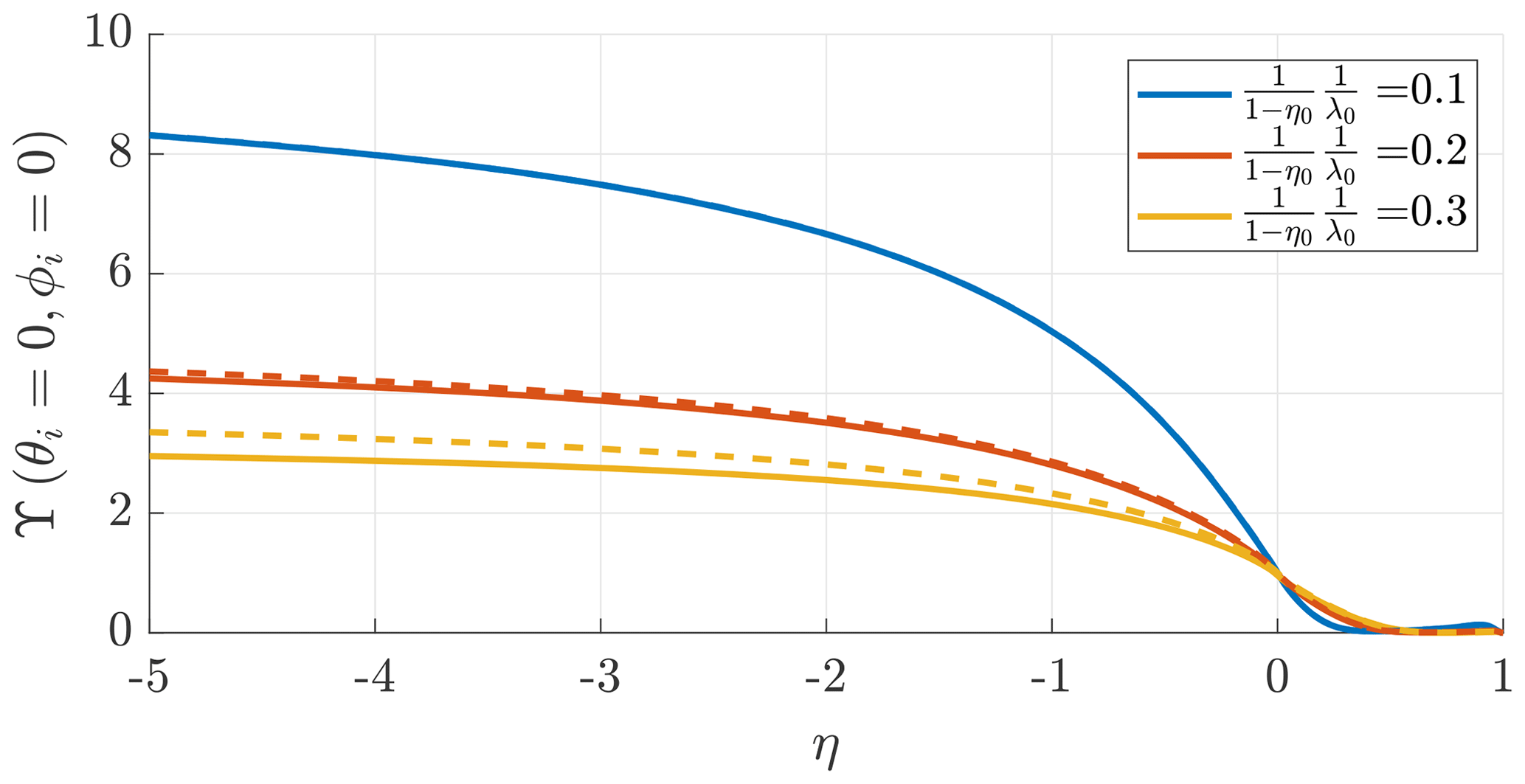
The integrals involved in Eq. (16) now have a closed-form solution, which will be used to derive a near- and a far-wake model in the next sections. This expression is derived by assuming that the angular distance of evaluation point p_j from the filament origin (i.e., θ_j and ϕ_j) is small, which is the case when the velocities induced by the vortex filaments trailed by the AWES are evaluated on the AWES itself, and by approximating the helicoidal vortex filament in Fig. 2a with the vortex ring system of Fig. 2b to compute the induction, which is a good idealization when the normalized torsional parameters λ₀ of the helicoidal vortex filament are large.

3 Near-wake model

In Sect. 2, the axial induced velocity produced by a helical vortex filament is modeled as half a vortex ring plus a semi-infinite vortex ring cascade, as in Fig. 2b. In this section, a near-wake model is developed based on this idealization. The velocities induced at the AWES by the near vortex filaments trailed by the AWES itself are studied here so that values of η (Eq. 2) are expected and consequently assumed to be small.

This section is organized as follows: in Sect. 3.1, the closed-form solution of the velocity induced by the near vortex filament and its linearized version are derived. In Sect. 3.2, the circulation of an elliptic wing flying in a circular trajectory is introduced to find the related trailed vorticity. In Sect. 3.3, the velocities induced by the trailed vortices on the lifting line of the elliptic wing are found. This allows for defining an induced drag coefficient modeling the near wake.

3.1 Velocity induced by the near vortex filament

The axial velocity at point p_j induced by the near vortex filament of intensity dΓ is (Eq. 16)

$$\begin{array}{}\text{(17)}& \begin{array}{rl}d{w}_{j,\mathrm{f}}^{\mathrm{n}}& =-{\displaystyle \frac{d\mathrm{\Gamma }}{\mathrm{4}\mathit{\pi }\mathrm{\Delta }R}}\\ & \underset{\mathrm{0}}{\overset{\mathit{\pi }}{\int }}{\displaystyle \frac{\mathit{\eta }(\mathrm{1}-\mathit{\eta })\left(\cos \left(\mathit{\theta }-{\mathit{\theta }}_j\right)-(\mathrm{1}-\mathit{\eta })\right)}{{\left(\mathrm{1}-\mathrm{2}(\mathrm{1}-\mathit{\eta })\cos \left(\mathit{\theta }-{\mathit{\theta }}_j\right)+(\mathrm{1}-\mathit{\eta }{)}^{\mathrm{2}}\right)}^{\frac{\mathrm{3}}{\mathrm{2}}}}}\mathrm{d}\mathit{\theta }\\ & =-{\displaystyle \frac{d\mathrm{\Gamma }}{\mathrm{4}\mathit{\pi }\mathrm{\Delta }R}}{\mathrm{{\rm Y}}}^{\mathrm{n}}\left(\mathit{\eta },{\mathit{\theta }}_j\right).\end{array}\end{array}$$

By changing the integration variable to ${\mathit{\theta }}^{*}=\mathit{\theta }-{\mathit{\theta }}_j$ and performing the integration, the shape factor of the near vortex filament Υⁿ has a closed-form solution:

$$\begin{array}{}\text{(18)}& \begin{array}{rl}{\mathrm{{\rm Y}}}^{\mathrm{n}}\left(\mathit{\eta },{\mathit{\theta }}_j\right)& =\underset{-{\mathit{\theta }}_j}{\overset{\mathit{\pi }-{\mathit{\theta }}_j}{\int }}{\displaystyle \frac{\mathit{\eta }(\mathrm{1}-\mathit{\eta })\left(\cos \left({\mathit{\theta }}^{*}\right)-(\mathrm{1}-\mathit{\eta })\right)}{{\left(\mathrm{1}-\mathrm{2}(\mathrm{1}-\mathit{\eta })\cos \left({\mathit{\theta }}^{*}\right)+(\mathrm{1}-\mathit{\eta }{)}^{\mathrm{2}}\right)}^{\frac{\mathrm{3}}{\mathrm{2}}}}}d{\mathit{\theta }}^{*}\\ & =-\left[{\displaystyle \frac{\mathit{\eta }}{\left|\mathit{\eta }\right|}}\left(K\left({\displaystyle \frac{{\mathit{\theta }}^{*}}{\mathrm{2}}}|m\right)+{\displaystyle \frac{\mathit{\eta }}{(\mathit{\eta }-\mathrm{2})}}E\left({\displaystyle \frac{{\mathit{\theta }}^{*}}{\mathrm{2}}}|m\right)\right)\right.\\ & {\left.-{\displaystyle \frac{\mathit{\eta }-\mathrm{1}}{\mathit{\eta }-\mathrm{2}}}{\displaystyle \frac{\mathrm{2}\sin \left({\mathit{\theta }}^{*}\right)}{\sqrt{{\mathit{\eta }}^{\mathrm{2}}+\mathrm{2}(\mathit{\eta }-\mathrm{1})\left(\cos \left({\mathit{\theta }}^{*}\right)-\mathrm{1}\right)}}}\right]}_{-{\mathit{\theta }}_j}^{\mathit{\pi }-{\mathit{\theta }}_j},\end{array}\end{array}$$

where $K\left(\frac{{\mathit{\theta }}^{*}}{\mathrm{2}}|m\right)$ is the incomplete elliptic integral of the first kind and $E\left(\frac{{\mathit{\theta }}^{*}}{\mathrm{2}}|m\right)$ is the incomplete elliptic integral of the second kind with $m=\mathrm{4}\frac{(\mathit{\eta }-\mathrm{1})}{{\mathit{\eta }}^{\mathrm{2}}}$. As θ_j is assumed to be small throughout all this work, Eq. (18) can be linearized with respect to θ_j as

$$\begin{array}{}\text{(19)}& \begin{array}{rl}{\mathrm{{\rm Y}}}^{\mathrm{n}}\left(\mathit{\eta },{\mathit{\theta }}_j\right)& \approx -{\displaystyle \frac{\mathit{\eta }}{\left|\mathit{\eta }\right|}}\left(K\left({\displaystyle \frac{\mathit{\pi }}{\mathrm{2}}}|m\right)+{\displaystyle \frac{\mathit{\eta }}{(\mathit{\eta }-\mathrm{2})}}E\left({\displaystyle \frac{\mathit{\pi }}{\mathrm{2}}}|m\right)\right)\\ & +{\displaystyle \frac{\mathit{\eta }-\mathrm{1}}{\mathit{\eta }-\mathrm{2}}}{\displaystyle \frac{\mathrm{2}{\mathit{\theta }}_j}{\sqrt{{\mathit{\eta }}^{\mathrm{2}}-(\mathit{\eta }-\mathrm{1}){\mathit{\theta }}_j^{\mathrm{2}}}}},\end{array}\end{array}$$

where $K\left(\frac{\mathit{\pi }}{\mathrm{2}}|m\right)$ and $E\left(\frac{\mathit{\pi }}{\mathrm{2}}|m\right)$ are the complete elliptic integral of the first and second kind respectively. Equation (19) can be linearized with respect to η, as its values for AWESs are expected to be small. Therefore, Υⁿ becomes

$$\begin{array}{}\text{(20)}& {\mathrm{{\rm Y}}}^{\mathrm{n}}\left(\mathit{\eta },{\mathit{\theta }}_j\right)\approx \mathrm{1}-\mathit{\eta }\left(\mathrm{1}-{\displaystyle \frac{\mathrm{1}}{\mathrm{4}}}\ln \left({\mathit{\eta }}^{\mathrm{2}}\right)\right)+{\displaystyle \frac{\mathit{\eta }-\mathrm{1}}{\mathit{\eta }-\mathrm{2}}}{\displaystyle \frac{\mathrm{2}{\mathit{\theta }}_j}{\sqrt{{\mathit{\eta }}^{\mathrm{2}}-(\mathit{\eta }-\mathrm{1}){\mathit{\theta }}_j^{\mathrm{2}}}}}.\end{array}$$

Figure 4 shows the trend of Υⁿ obtained with Eq. (18) (solid lines) and with the linearized version (Eq. 20) (dashed lines). The shape factor of the near vortex filament Υⁿ can be interpreted as a corrective factor to the solution of the straight vortex filament due to the filament curvature. If the evaluation point is in the same radial direction of the vortex filament origin (i.e., for θ_j=0), the following regions of η can be analyzed:

• η→1 is obtained for R_j≫R_f and Υⁿ→0, meaning that no velocities are induced;

• η>0 is obtained for R_j>R_f and Υⁿ<1, meaning that fewer velocities are induced compared to the straight-filament case;

• η→0 is obtained for R_j≈R_f or $(R_j\to \mathrm{\infty },R_{\mathrm{f}}\to \mathrm{\infty })$ and Υⁿ→1, meaning that the filament curvature is negligible and the solution coincides with the straight-filament case;

• η<0 is obtained for R_j<R_f and Υⁿ>1, meaning that more velocities are induced compared to the straight-filament case;

• $\mathit{\eta }\to -\mathrm{\infty }$ is obtained for R_j≪R_f and Υⁿ→π, as the evaluation point is close to the center of the half circle.

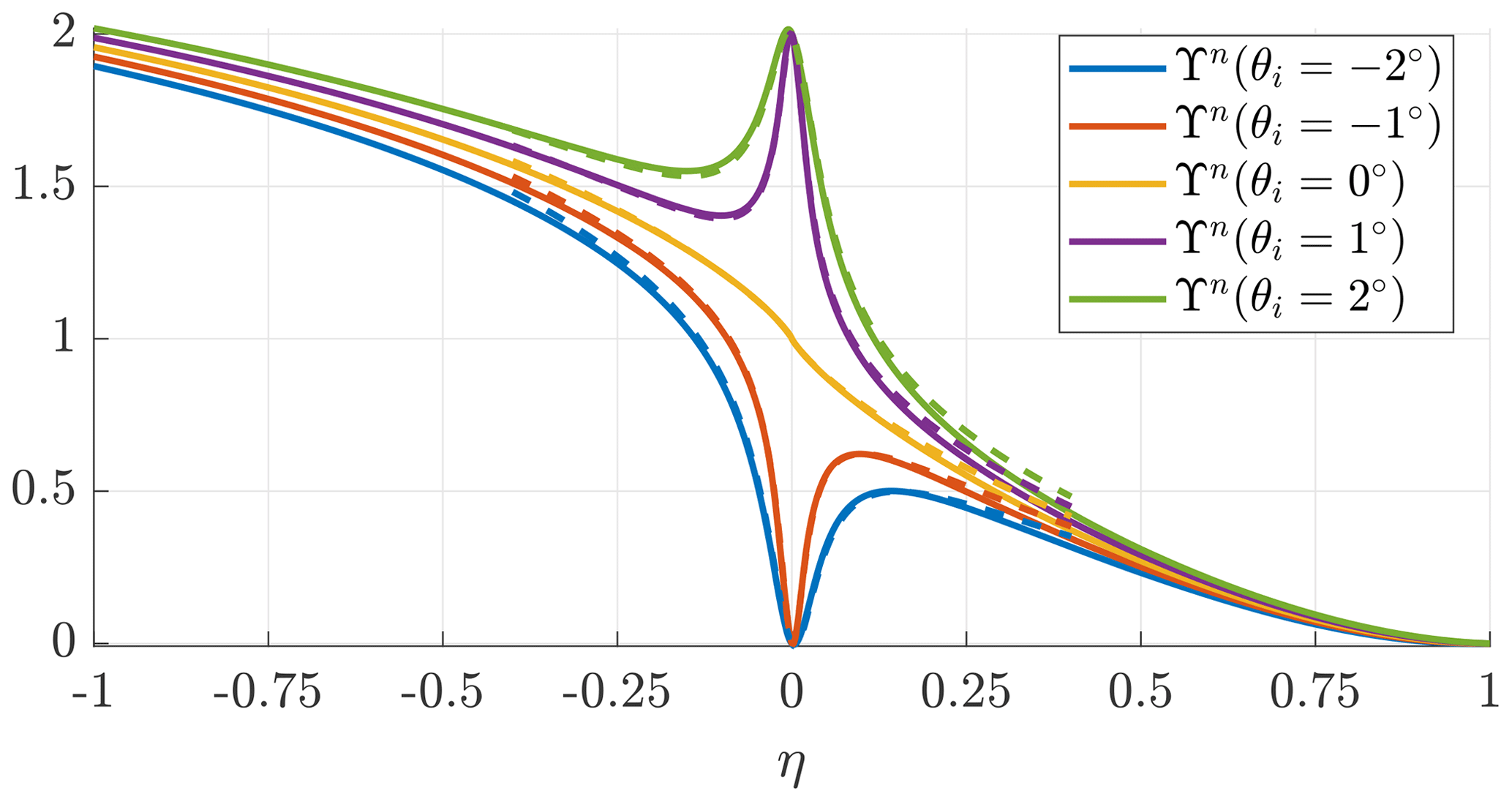
Figure 4 Shape factor of the near vortex filament Υⁿ as a function of η and θ_j for the complete solution (solid lines) and with the linearized version (dashed lines).

If the evaluation point is not in the same radial direction of the vortex filament origin (i.e., for θ_j≠0), the solution tends to Υⁿ(θ_j=0) when η→1 or $\mathit{\eta }\to -\mathrm{\infty }$ because the evaluation point is far from the filament, so the effect of θ_j vanishes. For θ_j>0, the evaluation point is downstream of the filament origin (see Fig. 2a) and Υⁿ→2 when η→0, meaning that twice the velocities induced by the semi-infinite straight filament (equivalent to one infinite straight filament) are found. For θ_j<0, the evaluation point is upstream of the filament origin and Υⁿ→0 when η→0, meaning that no velocities are induced.

3.2 Circulation trailed by an elliptic wing

Straight elliptical wings in forward flight have minimum induced drag and therefore are here chosen to analyze the near wake. To express the ratio between the wing coordinate $y_j=R_j-R_{\mathrm{0}}$ and the turning radius R₀, the parameter η_j is introduced as

$$\begin{array}{}\text{(21)}& {\mathit{\eta }}_j={\displaystyle \frac{y_j}{R_{\mathrm{0}}}}={\displaystyle \frac{R_j-R_{\mathrm{0}}}{R_{\mathrm{0}}}},\end{array}$$

for which at the outer wing tip $y_j=b/\mathrm{2}$ takes the value κ₀:

$$\begin{array}{}\text{(22)}& {\mathit{\kappa }}_{\mathrm{0}}={\displaystyle \frac{b/\mathrm{2}}{R_{\mathrm{0}}}},\end{array}$$

which is named the inverse turning ratio in this work.

The position of the trailed vorticity $y_{\mathrm{f}}=R_{\mathrm{f}}-R_{\mathrm{0}}$ is defined through the angular position α as

$$\begin{array}{}\text{(23)}& \cos \left(\mathit{\alpha }\right)={\displaystyle \frac{y_{\mathrm{f}}}{b/\mathrm{2}}}=-{\displaystyle \frac{{\mathit{\eta }}_{\mathrm{0}}}{{\mathit{\kappa }}_{\mathrm{0}}}},\end{array}$$

with η₀ defined in Eq. (3). The aerodynamic lift per unit length at the location of the trailed vorticity on the wing can be computed with the Kutta–Joukowski relation as

$$\begin{array}{}\text{(24)}& l\left(y_{\mathrm{f}}\right)=\mathit{\rho }u\mathrm{\Gamma },\end{array}$$

where ρ is the air density, Γ(y_f) is the bound circulation, and the velocity u is composed by the rigid-body velocity $u_{\mathrm{0}}\left(\frac{R_{\mathrm{0}}+y_{\mathrm{f}}}{R_{\mathrm{0}}}\right)=u_{\mathrm{0}}(\mathrm{1}-{\mathit{\eta }}_{\mathrm{0}})$ and the relative wind velocity v_r:

$$\begin{array}{}\text{(25)}& u\left(y_{\mathrm{f}}\right)=u_{\mathrm{0}}\left(\mathrm{1}-{\mathit{\eta }}_{\mathrm{0}}\right)\sqrt{\mathrm{1}+{\displaystyle \frac{v_{\mathrm{r}}^{\mathrm{2}}}{u_{\mathrm{0}}^{\mathrm{2}}{\left(\mathrm{1}-{\mathit{\eta }}_{\mathrm{0}}\right)}^{\mathrm{2}}}}},\end{array}$$

which can be approximated with the rigid-body velocity $u\left(y_{\mathrm{f}}\right)\approx u_{\mathrm{0}}(\mathrm{1}-{\mathit{\eta }}_{\mathrm{0}})$ for high wing speed ratios $\mathit{\lambda }=u_{\mathrm{0}}/v_{\mathrm{r}}$ and a small η₀. For the AWES to be in equilibrium, the total forces and moments needs to be null. Assuming that the roll moment ℒ is only due to the main wing lift¹, ℒ is

$$\begin{array}{}\text{(26)}& \mathcal{L}=\underset{-b/\mathrm{2}}{\overset{b/\mathrm{2}}{\int }}{y}_{\mathrm{f}}l\left(y_{\mathrm{f}}\right)\mathrm{d}{y}_{\mathrm{f}}=\mathit{\rho }{u}_{\mathrm{0}}\underset{-b/\mathrm{2}}{\overset{b/\mathrm{2}}{\int }}{y}_{\mathrm{f}}\left(\mathrm{1}-{\mathit{\eta }}_{\mathrm{0}}\right)\mathrm{\Gamma }\left(y_{\mathrm{f}}\right)\mathrm{d}{y}_{\mathrm{f}}=\mathrm{0}.\end{array}$$

The bound circulation Γ can be taken to set the lift distribution to be symmetric along the wing span:

$$\begin{array}{}\text{(27)}& \mathrm{\Gamma }={\displaystyle \frac{{\mathrm{\Gamma }}_{\parallel }}{\mathrm{1}-{\mathit{\eta }}_{\mathrm{0}}}}\approx {\mathrm{\Gamma }}_{\parallel }\left(\mathrm{1}+{\mathit{\eta }}_{\mathrm{0}}\right)={\mathrm{\Gamma }}_{\parallel }\left(\mathrm{1}-{\mathit{\kappa }}_{\mathrm{0}}\cos \mathit{\alpha }\right),\end{array}$$

where Γ_∥ is the symmetric circulation the wing would have in a straight motion and η₀ is assumed to be small. Note that loads are typically distributed along the wing span by means of ailerons, which create discontinuities in the lift distribution. The lift distribution is modeled here to be a continuous function for simplicity. The symmetric circulation the elliptic wing would have in forward flight Γ_∥ is (Anderson, 2017)

$$\begin{array}{}\text{(28)}& {\mathrm{\Gamma }}_{\parallel }={\mathrm{\Gamma }}_{\mathrm{0}}\sin \left(\mathit{\alpha }\right)=\mathrm{2}b{\displaystyle \frac{u_{\mathrm{0}}{C}_{\mathrm{L}}}{\mathit{\pi }\mathrm{AR}}}\sin \left(\mathit{\alpha }\right)=\mathrm{2}b{w}_{\parallel }\sin \left(\mathit{\alpha }\right),\end{array}$$

where C_L is the wing lift coefficient, AR is the wing aspect ratio and w_∥ is the induced velocity the same wing would have in forward flight.

The trailed vorticity, according to Helmholtz' law, is the derivative of the bound vorticity with respect to the wing span coordinate:

$$\begin{array}{}\text{(29)}& \mathit{\gamma }={\displaystyle \frac{\mathrm{d}\mathrm{\Gamma }}{\mathrm{d}{y}_{\mathrm{f}}}}={\mathrm{\Gamma }}_{\mathrm{0}}\left(\cos \left(\mathit{\alpha }\right)+{\mathit{\kappa }}_{\mathrm{0}}\left(\mathrm{1}-\mathrm{2}\cos (\mathit{\alpha }{)}^{\mathrm{2}}\right)\right){\displaystyle \frac{\mathrm{d}\mathit{\alpha }}{\mathrm{d}{y}_{\mathrm{f}}}}.\end{array}$$

3.3 Induced drag coefficient due to the near wake for an elliptic wing

The axial induced velocity $w_j^{\mathrm{n}}$ at a given point p_j along the lifting line (θ_j=0) due to the near wake is found by integrating the effects of the trailed vorticity γ along the wing span as

$$\begin{array}{}\text{(30)}& w_j^{\mathrm{n}}=-{\displaystyle \frac{\mathrm{1}}{\mathrm{4}\mathit{\pi }}}\underset{-b/\mathrm{2}}{\overset{b/\mathrm{2}}{\int }}{\displaystyle \frac{\mathit{\gamma }}{\mathrm{\Delta }R}}{\mathrm{{\rm Y}}}^{\mathrm{n}}\left(\mathit{\eta },{\mathit{\theta }}_j=\mathrm{0}\right)\mathrm{d}{y}_{\mathrm{f}}.\end{array}$$

The induced velocities on the lifting line can be found numerically and fitted between $y_j=-b/\mathrm{2}$ and $y_j=b/\mathrm{2}$. The induced velocity at a point on the lifting line given by the near wake is

$$\begin{array}{}\text{(31)}& w^{\mathrm{n}}\left({\mathit{\eta }}_j\right)=w_{\parallel }\left(\mathrm{1}-{\displaystyle \frac{\mathrm{3}}{\mathrm{2}}}{\mathit{\eta }}_j-{\mathit{\eta }}_j^{\mathrm{2}}+{\displaystyle \frac{{\mathit{\kappa }}_{\mathrm{0}}^{\mathrm{2}}}{\mathrm{4}}}\right).\end{array}$$

In Fig. 5, a comparison of the analytic approximation (Eq. 31) with the solutions obtained numerically is shown. The induction computed with straight vortex filaments or with the near vortex filaments are almost equivalent. This suggests that the development of lifting-line methods assuming straight trailed vortex filaments for time simulators (e.g., Damiani et al., 2019) or for flight dynamics analyses (e.g., Trevisi et al., 2021a) are a good approximation of the near wake for elliptic wings and for the inverse turning ratio κ₀ considered in the example or lower values. Recall that assuming straight trailed vortex filaments is equivalent to approximating ${\mathrm{{\rm Y}}}^{\mathrm{n}}(\mathit{\eta },{\mathit{\theta }}_j=\mathrm{0})$ in Eq. (30) with Υⁿ=1. Υⁿ goes to 1 for values of η going to 0, as shown in Fig. 4. Larger values of η in modulus are obtained for larger values of κ₀. For an increasing κ₀, the approximation of straight trailed vortex filaments is then expected to perform less well. Moreover, for wing types with more trailed vorticity near the wing tips (i.e., where values of η are larger in modulus), the approximation of straight trailed vortex filaments is also expected to perform less well.

Figure 5 Induced velocities computed analytically wⁿ (Eq. 31) and numerically with curved wake (Eq. 20 is used) and no-roll circulation w_∪(Γ), with straight wake and no-roll circulation w_∥(Γ), and with straight wake and symmetric circulation $w_{\parallel }\left({\mathrm{\Gamma }}_{\parallel }\right)$.

The induced change in the angle of attack for the local profile is

$$\begin{array}{}\text{(32)}& {\mathit{\alpha }}_i^{\mathrm{n}}\left({\mathit{\eta }}_j\right)={\displaystyle \frac{w^{\mathrm{n}}\left({\mathit{\eta }}_j\right)}{u\left({\mathit{\eta }}_j\right)}}={\displaystyle \frac{C_{\mathrm{L}}}{\mathit{\pi }\mathrm{AR}}}{\displaystyle \frac{\mathrm{1}}{\mathrm{1}+{\mathit{\eta }}_j}}\left(\mathrm{1}-{\displaystyle \frac{\mathrm{3}}{\mathrm{2}}}{\mathit{\eta }}_j-{\mathit{\eta }}_j^{\mathrm{2}}+{\displaystyle \frac{{\mathit{\kappa }}_{\mathrm{0}}^{\mathrm{2}}}{\mathrm{4}}}\right).\end{array}$$

Finally, the wing drag coefficient can be found by integrating the projection of the local lift coefficient along the velocity direction as

$$\begin{array}{}\text{(33)}& C_{\mathrm{Di}}^{\mathrm{n}}\approx {\displaystyle \frac{C_{\mathrm{L}}^{\mathrm{2}}}{\mathit{\pi }\mathrm{AR}}}\left(\mathrm{1}+{\displaystyle \frac{{\mathit{\kappa }}_{\mathrm{0}}^{\mathrm{2}}}{\mathrm{4}}}-{\displaystyle \frac{\mathrm{3}}{\mathrm{2}}}{\mathit{\kappa }}_{\mathrm{0}}^{\mathrm{3}}\right)\approx {\displaystyle \frac{C_{\mathrm{L}}^{\mathrm{2}}}{\mathit{\pi }\mathrm{AR}}},\end{array}$$

where κ₀ is assumed to be small. The induced drag of an elliptical wing, due to the near wake, is then found to be similar to the induced drag of the same wing in forward flight. The glide ratio related to the near-wake drag coefficient is

$$\begin{array}{}\text{(34)}& G^{\mathrm{n}}={\displaystyle \frac{C_{\mathrm{L}}}{C_{\mathrm{Di}}^{\mathrm{n}}}}\approx {\displaystyle \frac{\mathit{\pi }\mathrm{AR}}{C_{\mathrm{L}}}}.\end{array}$$

4 Far-wake model

In Sect. 2, the axial induced velocity produced by a helical vortex filament is modeled as half a vortex ring plus a semi-infinite vortex ring cascade, as in Fig. 2b. In Sect. 3, a near-wake model is built based on this idealization, while in this section a far-wake model is developed.

This section is organized as follows: in Sect. 4.1, an approximation of the velocities induced by two semi-infinite vortex ring cascades with opposite intensity is given as a function of their radial and axial distance. In Sect. 4.2, a drag coefficient modeling the far wake for an elliptic wing is found. In Sect. 4.3 an explicit closure model and in Sect. 4.4 an implicit closure model to find the vortex rings axial distance are introduced.

4.1 Velocity induced by the far vortex filaments

In the far wake, the wake is assumed to be already rolled up into two separate vortices, one for each of the wing tips. The velocities induced by the far wake are assumed to be constant over the wing span; therefore they are evaluated at the wing center of R_j=R₀. The velocity induced by the cascade of vortex rings of intensity Γ on the wing center is

$$\begin{array}{}\text{(35)}& \begin{array}{rl}{w}^{\mathrm{f}}& \approx -{\displaystyle \frac{\mathrm{\Gamma }}{\mathrm{4}\mathit{\pi }\mathrm{\Delta }R}}\sum _{k=\mathrm{1}}^{\mathrm{\infty }}\\ & \underset{{\mathrm{{\rm Y}}}_{z,k}^{\mathrm{f}}}{\underbrace{\underset{-\mathit{\pi }}{\overset{\mathit{\pi }}{\int }}{\displaystyle \frac{{\mathit{\eta }}_{\mathrm{0}}\left(\mathrm{1}-{\mathit{\eta }}_{\mathrm{0}}\right)\left(\cos \left(\mathit{\theta }\right)-\left(\mathrm{1}-{\mathit{\eta }}_{\mathrm{0}}\right)\right)}{{\left(\mathrm{1}-\mathrm{2}\left(\mathrm{1}-{\mathit{\eta }}_{\mathrm{0}}\right)\cos \left(\mathit{\theta }\right)+{\left(\mathrm{1}-{\mathit{\eta }}_{\mathrm{0}}\right)}^{\mathrm{2}}+{\left(\frac{\mathrm{2}\mathit{\pi }k}{{\mathit{\lambda }}_{\mathrm{0}}}\right)}^{\mathrm{2}}\right)}^{\frac{\mathrm{3}}{\mathrm{2}}}}}\mathrm{d}\mathit{\theta }}},\end{array}\end{array}$$

where ϕ_j in Eq. (16) is neglected. The integral has a closed-form solution, so ${\mathrm{{\rm Y}}}_{z,k}^{\mathrm{f}}$ takes the form

$$\begin{array}{}\text{(36)}& \begin{array}{rl}{\mathrm{{\rm Y}}}_{z,k}^{\mathrm{f}}\left({\mathit{\eta }}_{\mathrm{0}},{\mathit{\lambda }}_{\mathrm{0}}\right)=& {\displaystyle \frac{-\mathrm{2}{\mathit{\eta }}_{\mathrm{0}}}{{\left({\mathit{\eta }}_{\mathrm{0}}^{\mathrm{2}}+{\left(\frac{\mathrm{2}\mathit{\pi }k}{{\mathit{\lambda }}_{\mathrm{0}}}\right)}^{\mathrm{2}}\right)}^{\mathrm{1}/\mathrm{2}}}}\\ & \left(K\left(m\right)+{\displaystyle \frac{{\mathit{\eta }}_{\mathrm{0}}\left({\mathit{\eta }}_{\mathrm{0}}-\mathrm{2}\right)-{\left(\frac{\mathrm{2}\mathit{\pi }k}{{\mathit{\lambda }}_{\mathrm{0}}}\right)}^{\mathrm{2}}}{{\left({\mathit{\eta }}_{\mathrm{0}}-\mathrm{2}\right)}^{\mathrm{2}}+{\left(\frac{\mathrm{2}\mathit{\pi }k}{{\mathit{\lambda }}_{\mathrm{0}}}\right)}^{\mathrm{2}}}}E\left(m\right)\right),\end{array}\end{array}$$

with $m=\frac{\mathrm{4}({\mathit{\eta }}_{\mathrm{0}}-\mathrm{1})}{{\mathit{\eta }}_{\mathrm{0}}^{\mathrm{2}}+{\left(\frac{\mathrm{2}\mathit{\pi }k}{{\mathit{\lambda }}_{\mathrm{0}}}\right)}^{\mathrm{2}}}$².

The outer and inner trailed vortexes are assumed to be located at $R_{\mathrm{f}}=R_{\mathrm{0}}\pm y_{\mathrm{v}}$ such that $\mathrm{\Delta }R=\mp y_{\mathrm{v}}$ and ${\mathit{\eta }}_{\mathrm{0}}=\mp {\mathit{\eta }}_{\mathrm{v}}=\mp \frac{y_{\mathrm{v}}}{R_{\mathrm{0}}}$ with an intensity of $\mathrm{\Gamma }=\pm {\mathrm{\Gamma }}_{\mathrm{0}}$ respectively. The velocity at the wing center induced by the two vortex ring cascades is

$$\begin{array}{}\text{(37)}& \begin{array}{rl}{w}^{\mathrm{f}}& \approx {\displaystyle \frac{{\mathrm{\Gamma }}_{\mathrm{0}}}{\mathrm{4}\mathit{\pi }{y}_{\mathrm{v}}}}\left(\sum _{k=\mathrm{1}}^{\mathrm{\infty }}{\mathrm{{\rm Y}}}_{z,k}^{\mathrm{f}}\left({\mathit{\eta }}_{\mathrm{0}}=-{\mathit{\eta }}_{\mathrm{v}},{\mathit{\lambda }}_{\mathrm{0}}\right)\right.\\ & \left.+\sum _{k=\mathrm{1}}^{\mathrm{\infty }}{\mathrm{{\rm Y}}}_{z,k}^{\mathrm{f}}\left({\mathit{\eta }}_{\mathrm{0}}={\mathit{\eta }}_{\mathrm{v}},{\mathit{\lambda }}_{\mathrm{0}}\right)\right).\end{array}\end{array}$$

The summations can be solved numerically for different values of λ₀ and η_v, and its solution can be fitted as a function of these two parameters. The approximated solution of the summation is

$$\begin{array}{}\text{(38)}& \sum _{k=\mathrm{1}}^{\mathrm{\infty }}\left({\mathrm{{\rm Y}}}_{z,k}^{\mathrm{f}}\left(-{\mathit{\eta }}_{\mathrm{v}},{\mathit{\lambda }}_{\mathrm{0}}\right)+{\mathrm{{\rm Y}}}_{z,k}^{\mathrm{f}}\left({\mathit{\eta }}_{\mathrm{v}},{\mathit{\lambda }}_{\mathrm{0}}\right)\right)\approx {\displaystyle \frac{\mathrm{9}}{\mathrm{2}}}{\mathit{\eta }}_{\mathrm{v}}^{\mathit{\pi }/\mathrm{2}}{\left({\displaystyle \frac{{\mathit{\lambda }}_{\mathrm{0}}}{\mathrm{2}\mathit{\pi }}}\right)}^{\mathrm{3}/\mathrm{2}}.\end{array}$$

Figure 6 shows the comparison between the solution obtained numerically and the approximation given in Eq. (38).

Figure 6 Summation modeling the far-wake shape function obtained numerically (solid) and the fitted function (dashed).

4.2 Induced drag coefficient due to the far wake for an elliptic wing

For an elliptical wing, the rolled-up trailed vortices are located approximately at the center of trailed vorticity $y_{\mathrm{v}}=\frac{\mathit{\pi }}{\mathrm{8}}b$ (Gaunaa et al., 2020) for the outer and inner wing respectively such that their non-dimensional radial coordinate is ${\mathit{\eta }}_{\mathrm{v}}=\frac{\mathit{\pi }b}{\mathrm{8}{R}_{\mathrm{0}}}=\frac{\mathit{\pi }}{\mathrm{4}}{\mathit{\kappa }}_{\mathrm{0}}$. The approximate solution for the induced velocity, using the fitted solution of Eq. (38) into Eq. (37) and considering ${\mathrm{\Gamma }}_{\mathrm{0}}=\mathrm{2}b\frac{u_{\mathrm{0}}{C}_{\mathrm{L}}}{\mathit{\pi }\mathrm{AR}}$, is

$$\begin{array}{}\text{(39)}& w^{\mathrm{f}}\approx {\displaystyle \frac{\mathrm{1}}{\mathrm{4}\mathit{\pi }}}{\displaystyle \frac{u_{\mathrm{0}}{C}_{\mathrm{L}}}{\mathit{\pi }\mathrm{AR}}}{\mathit{\kappa }}_{\mathrm{0}}^{\mathit{\pi }/\mathrm{2}}{\mathit{\lambda }}_{\mathrm{0}}^{\mathrm{3}/\mathrm{2}},\end{array}$$

and the relative induced drag coefficient due to the far wake is

$$\begin{array}{}\text{(40)}& C_{\mathrm{Di}}^{\mathrm{f}}\approx {\displaystyle \frac{\mathrm{1}}{\mathrm{4}\mathit{\pi }}}{\displaystyle \frac{C_{\mathrm{L}}^{\mathrm{2}}}{\mathit{\pi }\mathrm{AR}}}{\mathit{\kappa }}_{\mathrm{0}}^{\mathit{\pi }/\mathrm{2}}{\mathit{\lambda }}_{\mathrm{0}}^{\mathrm{3}/\mathrm{2}}.\end{array}$$

The glide ratio related to the far-wake drag coefficient is

$$\begin{array}{}\text{(41)}& G^{\mathrm{f}}={\displaystyle \frac{C_{\mathrm{L}}}{C_{\mathrm{Di}}^{\mathrm{f}}}}\approx {\displaystyle \frac{\mathrm{4}\mathit{\pi }}{{\mathit{\kappa }}_{\mathrm{0}}^{\mathit{\pi }/\mathrm{2}}{\mathit{\lambda }}_{\mathrm{0}}^{\mathrm{3}/\mathrm{2}}}}{\displaystyle \frac{\mathit{\pi }\mathrm{AR}}{C_{\mathrm{L}}}}.\end{array}$$

As one of the final goals of this work is to model the system glide ratio G to refine a power equation by properly including the contribution from the wake, the correct drag coefficient shall include contributions from the near and far wake. The system glide ratio is therefore

$$\begin{array}{}\text{(42)}& G={\displaystyle \frac{C_{\mathrm{L}}}{C_{\mathrm{D}}}}={\displaystyle \frac{C_{\mathrm{L}}}{C_{\mathrm{D}\mathrm{0}}+C_{\mathrm{Di}}^{\mathrm{n}}+C_{\mathrm{Di}}^{\mathrm{f}}}}={\displaystyle \frac{\mathrm{1}}{\frac{\mathrm{1}}{G_{\mathrm{0}}}+\frac{\mathrm{1}}{G^{\mathrm{n}}}+\frac{\mathrm{1}}{G^{\mathrm{f}}}}},\end{array}$$

where C_D0 is the summation of the aircraft viscous and pressure drag C_D,v and the equivalent tether drag $C_{\mathrm{D},\mathrm{t}}=C_{⟂}\frac{D_{\mathrm{t}}{L}_{\mathrm{t}}}{\mathrm{4}A}$, where C_⟂ is the drag coefficient of the tether section, D_t and L_t are the tether diameter and length and A is the main wing area (Trevisi et al., 2020a).

The system glide ratio can be then seen as the sum of G₀, Gⁿ and G^f connected in parallel (as resistors connected in parallel in an electric circuit) as

$$\begin{array}{}\text{(43)}& G=G_{\mathrm{0}}\parallel G^{\mathrm{n}}\parallel G^{\mathrm{f}}={\displaystyle \frac{\mathrm{1}}{\frac{\mathrm{1}}{G_{\mathrm{0}}}+\frac{C_{\mathrm{L}}}{\mathit{\pi }\mathrm{AR}}+\frac{\mathrm{1}}{\mathrm{4}\mathit{\pi }}\frac{C_{\mathrm{L}}}{\mathit{\pi }\mathrm{AR}}{\mathit{\kappa }}_{\mathrm{0}}^{\mathit{\pi }/\mathrm{2}}{\mathit{\lambda }}_{\mathrm{0}}^{\mathrm{3}/\mathrm{2}}}}.\end{array}$$

Equation (43) models the system glide ratio of an AWES with an elliptic wing under the assumption of no wake expansion for a generic normalized torsional parameter λ₀. A closure model is then necessary to link λ₀ with the other aerodynamic and geometric parameters of the model. Two closure models are proposed in the following two sections.

4.3 Explicit closure model for the normalized torsional parameter

The first closure model assumes that the axial velocity of the vortex filaments is equal to the axial velocity at the AWES, similar to what assumed by de Vaal et al. (2014) in the derivation of a free-vortex wake model for wind turbines based on vortex ring elements. The axial velocity of the vortex filaments is assumed to be v_r(1−a_z), where a_z is the axial induction at the AWES wing center. The helix pitch h₀ can be approximated with the distance covered by the vortex filaments moving downwind in the revolution period. The revolution period is the ratio between the circumference length and the AWES mid-span tangential velocity $\frac{\mathrm{2}\mathit{\pi }{R}_{\mathrm{0}}}{u_{\mathrm{0}}}$:

$$\begin{array}{}\text{(44)}& h_{\mathrm{0}}=v_{\mathrm{r}}\left(\mathrm{1}-a_z\right){\displaystyle \frac{\mathrm{2}\mathit{\pi }{R}_{\mathrm{0}}}{u_{\mathrm{0}}}}={\displaystyle \frac{\mathrm{2}\mathit{\pi }{R}_{\mathrm{0}}}{\mathit{\lambda }}}\left(\mathrm{1}-a_z\right),\end{array}$$

where $\mathit{\lambda }=\frac{u_{\mathrm{0}}}{v_{\mathrm{r}}}$ is the wing speed ratio.

Considering the definition of the normalized torsional parameter ${\mathit{\lambda }}_{\mathrm{0}}=\frac{\mathrm{2}\mathit{\pi }{R}_{\mathrm{0}}}{h_{\mathrm{0}}}$ (Eq. 6), λ₀ can be linked to the wing speed ratio λ as

$$\begin{array}{}\text{(45)}& {\mathit{\lambda }}_{\mathrm{0}}={\displaystyle \frac{\mathit{\lambda }}{\left(\mathrm{1}-a_z\right)}}.\end{array}$$

The axial induction is the sum of the near-wake and the far-wake induced velocities, normalized with the relative wind speed:

$$\begin{array}{}\text{(46)}& a_z={\displaystyle \frac{w_{\mathrm{0}}^{\mathrm{n}}+w^{\mathrm{f}}}{v_{\mathrm{r}}}}=\mathit{\lambda }{\displaystyle \frac{C_{\mathrm{L}}}{\mathit{\pi }\mathrm{AR}}}\left(\mathrm{1}+{\displaystyle \frac{\mathrm{1}}{\mathrm{4}\mathit{\pi }}}{\mathit{\kappa }}_{\mathrm{0}}^{\mathit{\pi }/\mathrm{2}}{\mathit{\lambda }}_{\mathrm{0}}^{\mathrm{3}/\mathrm{2}}\right).\end{array}$$

By inserting the axial induction a_z into Eq. (45), the wing speed ratio λ is

$$\begin{array}{}\text{(47)}& \mathit{\lambda }={\mathit{\lambda }}_{\mathrm{0}}\left(\mathrm{1}-\mathit{\lambda }{\displaystyle \frac{C_{\mathrm{L}}}{\mathit{\pi }\mathrm{AR}}}\left(\mathrm{1}+{\displaystyle \frac{\mathrm{1}}{\mathrm{4}\mathit{\pi }}}{\mathit{\kappa }}_{\mathrm{0}}^{\mathit{\pi }/\mathrm{2}}{\mathit{\lambda }}_{\mathrm{0}}^{\mathrm{3}/\mathrm{2}}\right)\right),\end{array}$$

which can be rewritten as

$$\begin{array}{}\text{(48)}& \mathit{\lambda }={\displaystyle \frac{\mathrm{1}}{\frac{\mathrm{1}}{{\mathit{\lambda }}_{\mathrm{0}}}+\frac{C_{\mathrm{L}}}{\mathit{\pi }\mathrm{AR}}+\frac{\mathrm{1}}{\mathrm{4}\mathit{\pi }}\frac{C_{\mathrm{L}}}{\mathit{\pi }\mathrm{AR}}{\mathit{\kappa }}_{\mathrm{0}}^{\mathit{\pi }/\mathrm{2}}{\mathit{\lambda }}_{\mathrm{0}}^{\mathrm{3}/\mathrm{2}}}}.\end{array}$$

This equation links λ (wing speed ratio) to λ₀ (normalized torsional parameter of the helicoidal wake) and to the induced change in the angle of attack produced by the near wake $\frac{C_{\mathrm{L}}}{\mathit{\pi }\mathrm{AR}}$ and by the far wake $\frac{\mathrm{1}}{\mathrm{4}\mathit{\pi }}\frac{C_{\mathrm{L}}}{\mathit{\pi }\mathrm{AR}}{\mathit{\kappa }}_{\mathrm{0}}^{\mathit{\pi }/\mathrm{2}}{\mathit{\lambda }}_{\mathrm{0}}^{\mathrm{3}/\mathrm{2}}$.

Figure 7 Velocity triangles and force balance (a) if the effect of the induced velocities is taken into account by including induced drag terms and (b) if the effect of the induced velocities is taken into account by reducing the incoming wind.

For AWES flying crosswind in steady state the propulsive lift is balanced by the drag such that the force balance along the AWES longitudinal direction is null. The glide ratio G is then equal to the wing speed ratio λ (Fig. 7a). By setting equal Eqs. (43) and (48), G₀ is found to be equal to λ₀. This means that the normalized torsional parameter of the helicoidal wake λ₀ is equal to the glide ratio related to the constant drag term G₀. A graphical representation of this equality is given in Fig. 7b. λ₀ is the ratio between the AWES longitudinal velocity and the wind velocity reduced by the induced velocities at the AWES (Eq. 45). If the induced velocities due to the near and far wake are subtracted from the incoming wind, the induced drag related to the near and far wake should not be considered in the drag evaluation. Therefore, the only remaining drag term is related to the drag at zero lift. For the AWES to be in equilibrium along the longitudinal direction, λ₀ needs to be equal to G₀. Note that the two sketches in Fig. 7 show the same physics. In Fig. 7a the effect of the induced velocities is taken into account by including induced drag terms, as typically done for flying wings. In Fig. 7b the effect of the induced velocities is taken into account by reducing the incoming wind, as typically done for wind turbines. The resultant longitudinal velocity u₀ is equal for the two sketches.

The system glide ratio (Eq. 43) can then be formulated by considering λ₀=G₀, leading to a new definition:

$$\begin{array}{}\text{(49)}& G={\displaystyle \frac{\mathrm{1}}{\frac{\mathrm{1}}{G_{\mathrm{0}}}+\frac{C_{\mathrm{L}}}{\mathit{\pi }\mathrm{AR}}+\frac{\mathrm{1}}{\mathrm{4}\mathit{\pi }}\frac{C_{\mathrm{L}}}{\mathit{\pi }\mathrm{AR}}{\mathit{\kappa }}_{\mathrm{0}}^{\mathit{\pi }/\mathrm{2}}{G}_{\mathrm{0}}^{\mathrm{3}/\mathrm{2}}}}.\end{array}$$

The system glide ratio is now also dependent on the flight trajectory radius through the inverse turning ratio κ₀. For a large turning radius (i.e., small κ₀) the contribution from the far wake vanishes and Eq. (49) coincides with the glide ratio expression for the same wing in straight motion.

Figure 8 shows the ratio between the far- and near-wake induced drag (i.e., the expression $\frac{\mathrm{1}}{\mathrm{4}\mathit{\pi }}{\mathit{\kappa }}_{\mathrm{0}}^{\mathit{\pi }/\mathrm{2}}{G}_{\mathrm{0}}^{\mathrm{3}/\mathrm{2}}$). AWES designs tend to have high values of G₀, obtained by minimizing C_D0 and operating at high lift coefficient C_L, and to have a large κ₀ (i.e., small turning radius R₀). Small turning radii minimize the vertical height of the trajectory and therefore reduce the potential energy exchange over the loop, reducing power losses (Trevisi et al., 2022a). The induction of the far wake however penalizes solutions with high G₀ and high κ₀, highlighting the need of a trade-off between different disciplines in the design. These considerations, among others, justify the development of the multidisciplinary design, analysis and optimization framework T-GliDe (Trevisi et al., 2022b).

Figure 8 Ratio between the far- and near-wake induced drag as a function of the glide ratio related to C_D0 and the inverse turning ratio κ₀.

In Sect. 5, a comparison between the results produced by this closure model and by a lifting-line free-vortex wake method, implemented in QBlade, is performed. Unfortunately, the comparison does not show a satisfactory agreement between the two methods for high-loading cases. Therefore, an implicit closure model is proposed in the next section.

4.4 Implicit closure model for the normalized torsional parameter

The second proposed closure model for the normalized torsional parameter estimates the wake velocity by considering the axial and the radial induced velocities at the AWES. It is assumed that the velocity of the vortex filaments in the far wake is equal in modulus to their velocity when they are trailed (i.e., at the AWES). The velocity at the AWES is composed by the axial velocity v_r(1−a_z) and by the radial velocity v_ra_r. Note that the radial velocity is only due to velocities induced from the far wake. The helix pitch h₀ can then be found by considering that the axial velocity of the far vortex filaments is $v_{\mathrm{r}}\sqrt{(\mathrm{1}-a_z{)}^{\mathrm{2}}+a_{\mathrm{r}}^{\mathrm{2}}}$:

$$\begin{array}{}\text{(50)}& h_{\mathrm{0}}=v_{\mathrm{r}}\sqrt{{\left(\mathrm{1}-a_z\right)}^{\mathrm{2}}+a_{\mathrm{r}}^{\mathrm{2}}}{\displaystyle \frac{\mathrm{2}\mathit{\pi }{R}_{\mathrm{0}}}{u_{\mathrm{0}}}}={\displaystyle \frac{\mathrm{2}\mathit{\pi }{R}_{\mathrm{0}}}{\mathit{\lambda }}}\sqrt{{\left(\mathrm{1}-a_z\right)}^{\mathrm{2}}+a_{\mathrm{r}}^{\mathrm{2}}}.\end{array}$$

The normalized torsional parameter can then be written as

$$\begin{array}{}\text{(51)}& {\mathit{\lambda }}_{\mathrm{0}}={\displaystyle \frac{\mathit{\lambda }}{\sqrt{{\left(\mathrm{1}-a_z\right)}^{\mathrm{2}}+a_{\mathrm{r}}^{\mathrm{2}}}}},\end{array}$$

where a_z is given in Eq. (46) and a_r for an elliptic wing can be approximated as (see Appendix A for the derivation)

$$\begin{array}{}\text{(52)}& a_{\mathrm{r}}\approx \mathit{\lambda }{\displaystyle \frac{\mathrm{2}}{\mathrm{9}\mathit{\pi }}}{\displaystyle \frac{C_{\mathrm{L}}}{\mathit{\pi }\mathrm{AR}}}{\mathit{\kappa }}_{\mathrm{0}}^{\mathit{\pi }/\mathrm{2}}{\mathit{\lambda }}_{\mathrm{0}}^{\mathrm{1.1}}.\end{array}$$

The normalized torsional parameter (Eq. 51) can be found iteratively by considering the axial (Eq. 46) and the radial (Eq. 52) induction and the definition of the glide ratio (Eq. 43), which is equal to the wing speed ratio G=λ when the AWES is in equilibrium.

The estimation of radial induced velocities is important not only to compute the axial velocity of the far vortex filaments but also to estimate the AWES aerodynamic forces and moments. In the case of a straight wing with the wing span aligned with the radial direction (as in this paper), the radial induced velocities do not generate any aerodynamic force on the wing, as they are aligned with the span. On the contrary, the radial induced velocities generate aerodynamic forces and moments in the case of a straight wing with the span not aligned with the radial direction (i.e., the AWES is yawed or rolled) or in the case of a wing characterized by a dihedral and/or sweep angle. Moreover, the radial induced velocities also influence the angle of attack of the vertical stabilizer.

5 Comparison with a lifting-line free-vortex wake method

To validate the newly introduced aerodynamic model, a comparison with higher-fidelity code is needed. QBlade is chosen for the comparison, as it uses a thoroughly validated lifting-line free-vortex wake method (Marten et al., 2015) for the aerodynamic modeling of conventional wind turbines. The wake is modeled explicitly with Lagrangian vortex elements, resulting in a fully resolved velocity distribution around the AWES.

5.1 Lifting-line free-vortex wake setup

As QBlade is being used to validate the new model, the free-vortex wake model is idealized accordingly. The airfoils are described by idealized polars with constant drag coefficient C_D0 and a constant slope of the lift coefficient with respect to the angle of attack of $C_{l,\mathit{\alpha }}=\mathrm{2}\mathit{\pi }$. The AWES is modeled as a horizontal axis wind turbine with one blade and no tower. The hub radius of the wind turbine is set to be equal to the radial position of the inner wing tip. The elliptical wing is then defined in the blade definition. Large structural rigidity is given to avoid aeroelastic phenomena. Gravity is set to zero to look for steady results. The wing is discretized with 20 aerodynamic panels. For a given setup (C_D0, κ₀, AR), different lift coefficients can be obtained by pitching the wing. The wing is free to move on the circular trajectory so that its velocity is determined by the force equilibrium along the motion direction. Once quantities reach a constant value as a function of time, the wing speed ratio, which is equal to the glide ratio, is estimated from the rotational speed. The wing lift coefficient is obtained by knowing the thrust force produced and the rotational speed.

In Fig. 9, the wake shown in the graphic interface of QBlade is reported for a case with AR=20, κ₀=0.15, C_D0=0.05 and 0^∘ of pitch, which leads to C_L=0.55. A plane, defined by the AWES position and wake center, is used to visualize the axial velocity.

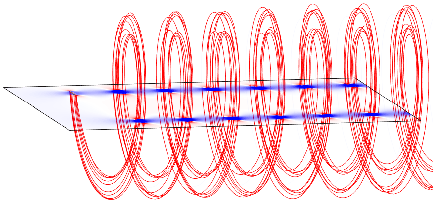
Figure 9 Wake shown in the graphic interface of QBlade for a case with AR=20, κ₀=0.15, C_D0=0.05 and C_L=0.55.

5.2 Comparison of the normalized torsional parameter

The first comparison concerns the downstream position of the vortices. The helix pitch can be found with $h_{\mathrm{0}}=\frac{\mathrm{2}\mathit{\pi }{R}_{\mathrm{0}}}{{\mathit{\lambda }}_{\mathrm{0}}}$ (Eq. 6), where λ₀ is the normalized torsional parameter. In this paper, an explicit (Sect. 4.3) and an implicit (Sect. 4.4) closure model for the normalized torsional parameter are proposed.

Figures 10 and 11 show the downstream vortex position, obtained by taking the curl of the velocity field, in the plane containing the AWES (see Fig. 9 for the plane illustration) for a setup with AR=20, κ₀=0.15 and C_D0=0.05. Figure 10 shows a low-loading case with C_L=0.55, while Fig. 11 shows a high-loading case with C_L=1.3. The blue vertical lines highlight the downstream position of the vortices predicted by the explicit model, while the black line is that of the implicit model. The dotted red lines highlight the radial position of the vortices assumed by the analytical model. For the low-loading case, both models accurately predict the vortex position. For the high-loading case, the implicit model greatly outperforms the explicit model, showing that the radial induced velocity at the AWES significantly contributes to the velocity of the far vortex filaments. In the high-loading case, the wake expands slightly due to the radial induced velocities. The wake expansion is neglected in the analytical modeling.

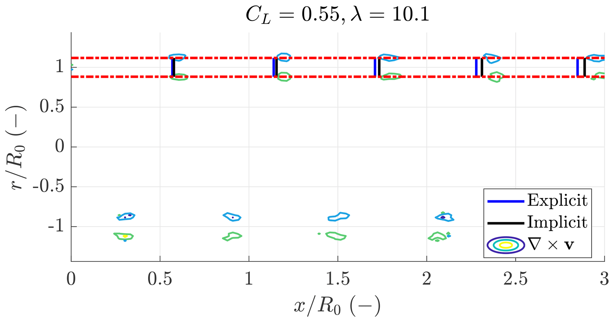
Figure 10 Downstream vortex position for a case with AR=20, κ₀=0.15 and C_D0=0.05 in a low-loading case with C_L=0.55 and λ=10.1.

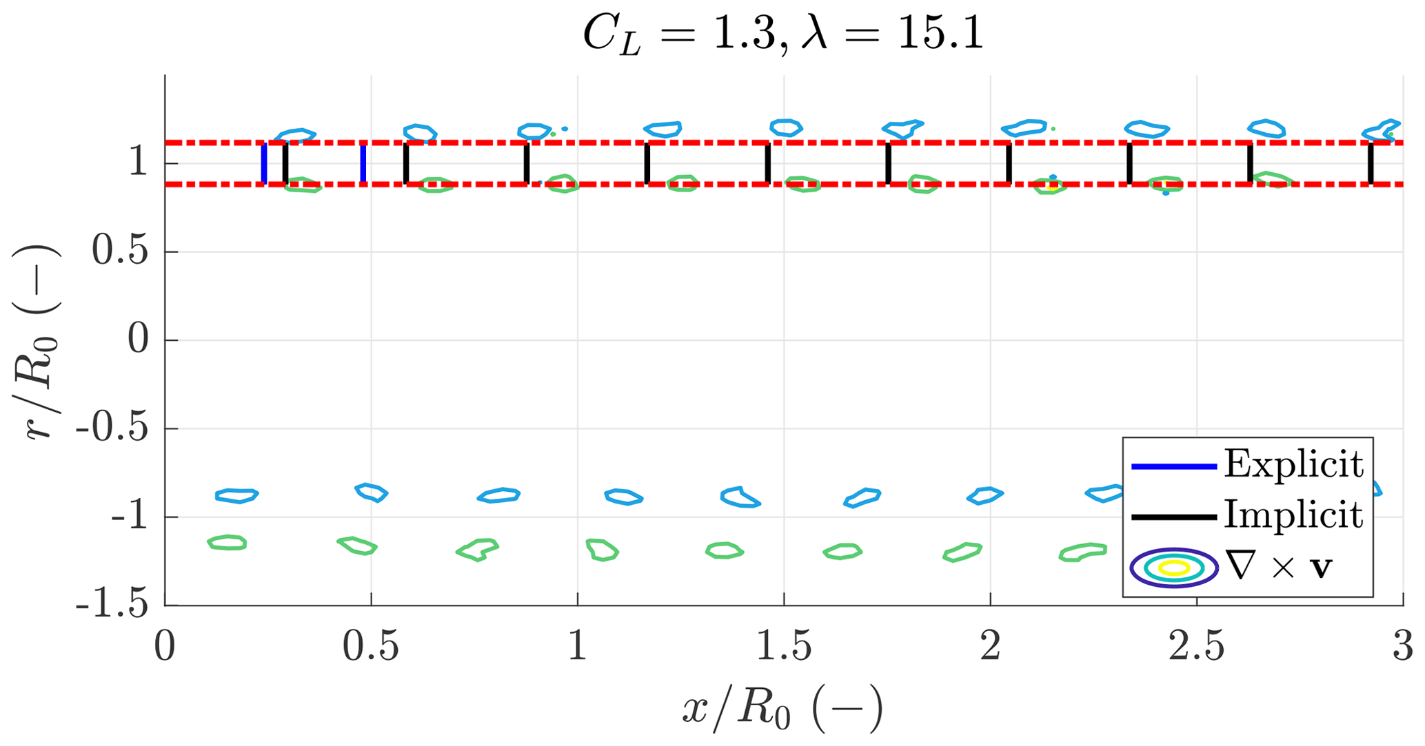
Figure 11 Downstream vortex position for a case with AR=20, κ₀=0.15 and C_D0=0.05 in a high-loading case with C_L=1.3 and λ=15.1. Only the position the first two vortices predicted by the explicit model is shown for clarity.

5.3 Comparison of axial induced velocities

In this section, the axial induced velocities computed with the analytical model just introduced and the implicit closure model are compared with the results of QBlade and two literature models related to the far wake. The high-loading case introduced in the previous section (AR=20, κ₀=0.15, C_D0=0.05 and C_L=1.3) is here used to show the results.

The bound circulation Γ is retrieved from QBlade, and the trailed vorticity γ can be obtained by differentiating the bound vorticity with respect to the spanwise coordinate. The induced velocities due to the near wake wⁿ can then be found by integrating Eq. (30) numerically. The induced velocities due to the far wake w^f are computed with Eq. (39).

The first model from the literature is the far-wake model by Gaunaa et al. (2020):

$$\begin{array}{}\text{(53)}& w_{\mathrm{G}.}^{\mathrm{f}}={\displaystyle \frac{u_{\mathrm{0}}{C}_{\mathrm{L}}}{\mathit{\pi }\mathrm{AR}}}{\displaystyle \frac{{\mathit{\kappa }}_{\mathrm{0}}^{\mathrm{2}}{G}^{\mathrm{2}}}{\mathrm{24}{\left(\mathrm{1}-\frac{\mathrm{4}G{C}_{\mathrm{L}}}{{\mathit{\pi }}^{\mathrm{3}}\mathrm{AR}}\right)}^{\mathrm{2}}}},\end{array}$$

where C_L is taken from QBlade and G is found iteratively. This model is coupled to the near-wake model introduced in this paper, as the near-wake model from Gaunaa et al. (2020) is tuned with CFD results and does not agree with the proposed near-wake model.

The second model from the literature, used to estimate the induction $a_{m.}^{\mathrm{f}}$, is the momentum-based model by Kheiri et al. (2018):

$$\begin{array}{}\text{(54)}& {\displaystyle \frac{a_{m.}^{\mathrm{f}}}{\mathrm{1}-a_{m.}^{\mathrm{f}}}}={\displaystyle \frac{{\mathit{\kappa }}_{\mathrm{0}}}{\mathrm{4}}}{\displaystyle \frac{C_{\mathrm{L}}}{\mathit{\pi }\mathrm{AR}}}{\left({\displaystyle \frac{C_{\mathrm{L}}}{C_{\mathrm{D},k}}}\right)}^{\mathrm{2}},\end{array}$$

where $C_{\mathrm{D},k}=C_{\mathrm{D}\mathrm{0}}+\frac{C_{\mathrm{L}}^{\mathrm{2}}}{\mathit{\pi }\mathrm{AR}}$ and C_L is taken from QBlade. Also this model is coupled to the near-wake model introduced in this paper such that $a_{m.}^{\mathrm{f}}$ can be seen as the induction applied to the 3D polars of the AWES.

Figure 12 shows the induction at the lifting line computed with QBlade, with the present model and with two models from the literature. The momentum-based model overestimates the induced velocities because a part of the wake is counted twice if the AWES is described by 3D polars, as explained by Gaunaa et al. (2020). The proposed model and the far wake from Gaunaa et al. (2020) coupled to the proposed near-wake model accurately predict the induction at the lifting line.

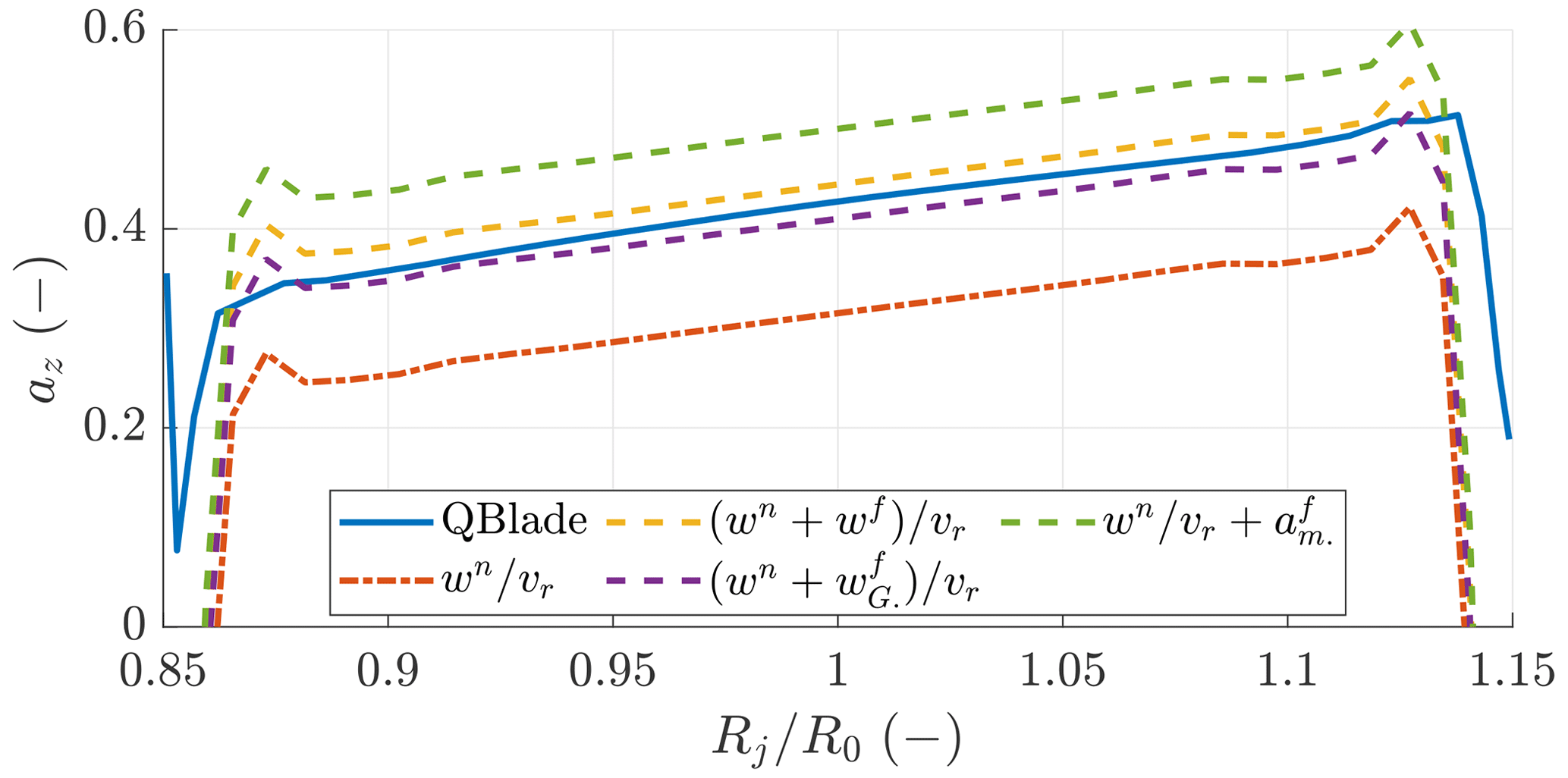
Figure 12 Axial induction at the lifting line obtained with QBlade (solid blue line), with the near-wake model introduced in this work $w^{\mathrm{n}}/v_{\mathrm{r}}$ coupled to the far-wake model introduced here $(w^{\mathrm{n}}+w^{\mathrm{f}})/v_{\mathrm{r}}$, to the far-wake model from Gaunaa et al. (2020) $(w^{\mathrm{n}}+w_{\mathrm{G}.}^{\mathrm{f}})/v_{\mathrm{r}}$ and to the momentum-based model $w^{\mathrm{n}}/v_{\mathrm{r}}+a_{m.}^{\mathrm{f}}$.

5.4 Comparison of radial induced velocities

In this section, the radial induced velocities computed with the analytical model (Eq. 52) are compared with the results of QBlade. Figure 13 shows the radial velocities for the high-loading case (AR=20, κ₀=0.15, C_D0=0.05 and C_L=1.3). A good agreement between the QBlade output and the analytic solution is found.

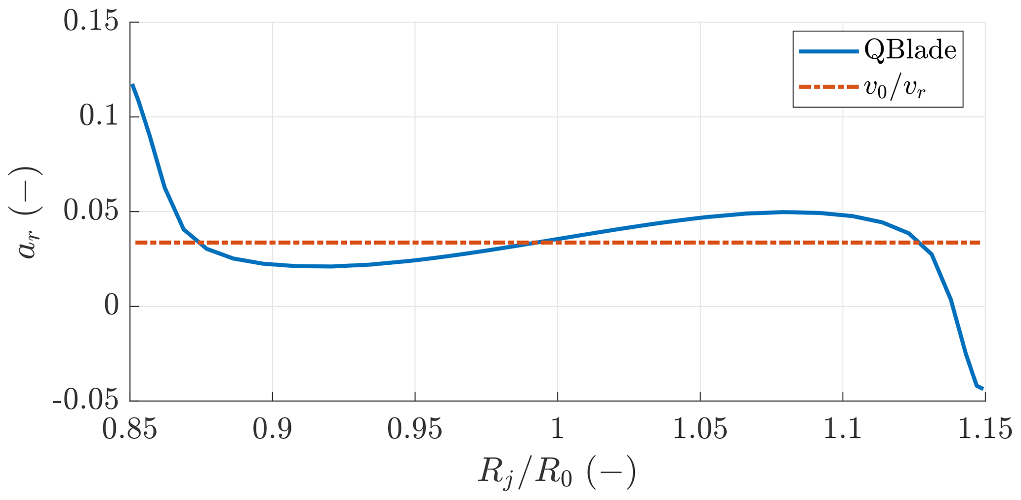
Figure 13 Radial induction at the lifting line obtained with QBlade (solid blue line) and with the analytic model (dash-dotted red line).

5.5 Comparison of axial induced velocities at the AWES tail

In this section, the axial induced velocities in the plane normal to the wing span passing by the center of the wing predicted with the proposed model and with a literature analytical model are compared with the results from QBlade.

The induced velocity in the symmetry plane of the AWES due to the trailed vorticity in the near wake can be found as a function of θ_j with

$$\begin{array}{}\text{(55)}& w_j^{\mathrm{n}}\left(\mathit{\eta }={\mathit{\eta }}_{\mathrm{0}},{\mathit{\theta }}_j\right)=-{\displaystyle \frac{\mathrm{1}}{\mathrm{4}\mathit{\pi }}}\underset{-b/\mathrm{2}}{\overset{b/\mathrm{2}}{\int }}{\displaystyle \frac{\mathit{\gamma }}{\mathrm{\Delta }R}}{\mathrm{{\rm Y}}}^{\mathrm{n}}\left(\mathit{\eta }={\mathit{\eta }}_{\mathrm{0}},{\mathit{\theta }}_j\right)\mathrm{d}{y}_{\mathrm{f}},\end{array}$$

where γ is taken from QBlade. To find the velocity field, the velocities induced by the bound vorticity Γ and from the far wake are considered too.

Phillips et al. (2002) study the velocities induced at the tail from a wing in forward flight. For an elliptical wing with no sweep, the induced velocities can be reformulated as

$$\begin{array}{}\text{(56)}& w_{\mathrm{i},\mathrm{Ph}.}=w_{\parallel }{\displaystyle \frac{\mathrm{8}}{{\mathit{\pi }}^{\mathrm{2}}}}\left(\mathrm{1}+{\displaystyle \frac{{\mathit{\theta }}_j^{\mathrm{2}}+{\left(\frac{\mathit{\pi }}{\mathrm{4}}{\mathit{\kappa }}_{\mathrm{0}}\right)}^{\mathrm{2}}}{{\mathit{\theta }}_j\sqrt{{\mathit{\theta }}_j^{\mathrm{2}}+{\left(\frac{\mathit{\pi }}{\mathrm{4}}{\mathit{\kappa }}_{\mathrm{0}}\right)}^{\mathrm{2}}}}}\right).\end{array}$$

As the velocities induced by the near wake are similar to the velocities induced by the wing in forward flight, the contribution from the far wake is added to this expression.

In Fig. 14, the induced change in the angle of attack found in QBlade is compared with the two solutions for the high-loading case (AR=20, κ₀=0.15, C_D0=0.05 and C_L=1.3). The proposed model is in good agreement with QBlade, and the model by Phillips et al. (2002) can still capture the main trend. These models can then be used to size the horizontal stabilizer.

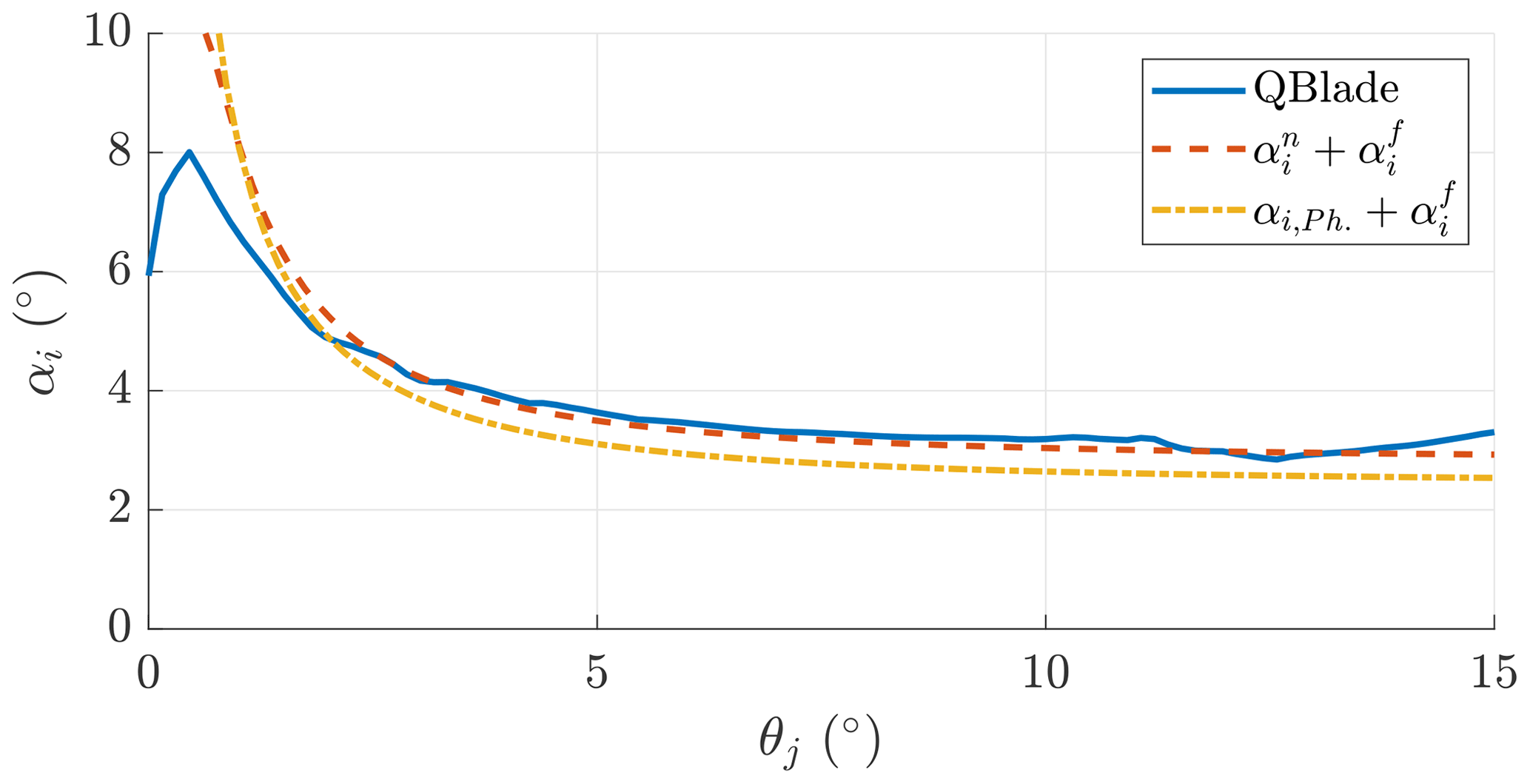
Figure 14 Induced change in the angle of attack from QBlade (solid blue line) compared with the proposed model (dashed red line) and the analytical solution from Phillips et al. (2002) (dash-dotted yellow line) for a wing in forward flight.

5.6 Comparison of glide ratios

The estimation of the system glide ratio is crucial for power production estimation. Figure 15 shows the glide ratio as a function of the lift coefficient for a case with AR=20, κ₀=0.15 and C_D0=0.05 computed considering straight wakes (G₀∥Gⁿ), the explicit model ($G_{\mathrm{0}}\parallel G^{\mathrm{n}}\parallel G_{\mathrm{expl}}^{\mathrm{f}}$, Eq. 49), the implicit model ($G_{\mathrm{0}}\parallel G^{\mathrm{n}}\parallel G_{\mathrm{impl}}^{\mathrm{f}}$, Sect. 4.4) and the far-wake model from Gaunaa et al. (2020) coupled to the proposed near wake ($G_{\mathrm{0}}\parallel G^{\mathrm{n}}\parallel G_{\mathrm{G}.}^{\mathrm{f}}$). The squares are the solutions obtained with QBlade. The explicit closure model results in a conservative glide ratio estimation for high loading, as it predicts the helix pitch to be smaller than what is found in QBlade. Using the implicit closure model and the model from Gaunaa et al. (2020) for the far wake results in accurate prediction of the results of QBlade.

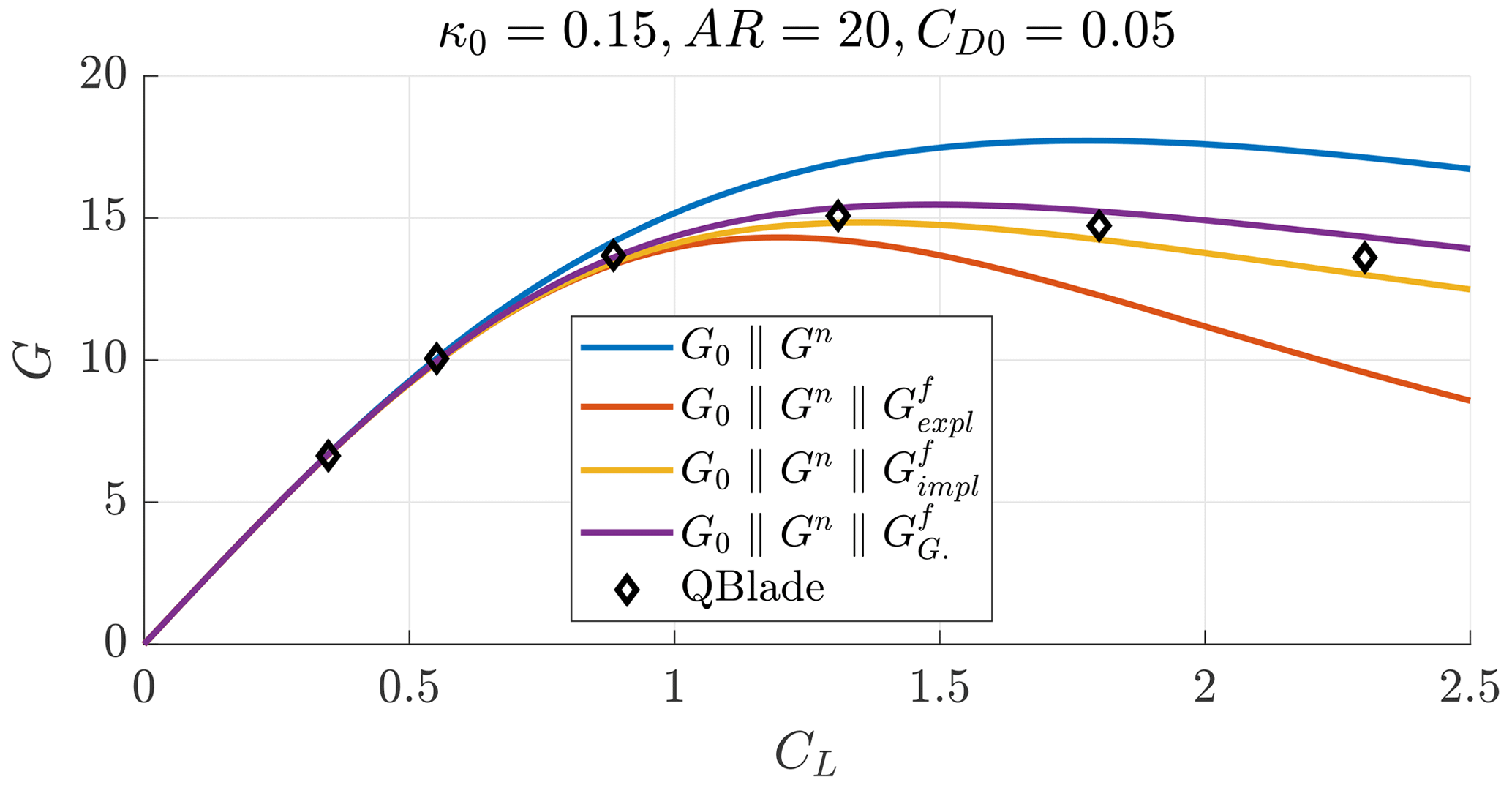
Figure 15 Glide ratio as a function of the lift coefficient for a case with AR=20, κ₀=0.15 and C_D0=0.05.

In Appendix B, more validation cases are reported. Generally, the implicit closure model results in an underestimation of the QBlade glide ratio estimation, while the model from Gaunaa et al. (2020) in an overestimation. The two methods are in accord and have the same computational cost.

6 Conclusions

In this work, a detailed analysis of the airborne wind energy system (AWES) aerodynamic wake is carried out with vortex methods and models to find the induced velocities at the AWES.

Under the assumption of steady crosswind operations and a non-expanding wake, the expression for the velocities induced in the neighborhood of the AWES from a helicoidal vortex filament, trailed by a position on the AWES wing, is divided into an expression modeling the near vortex filament and one for the far vortex filament.

The near vortex filament is modeled as the first half rotation of the helicoidal filament, where the axial component of the filament is neglected. The velocity induced by the near vortex filament is expressed in terms of elliptic integrals, and it is linearized to a more intuitive expression. The induced drag coefficient modeling the near wake, built up from the contributions of the near vortex filaments, is found to be similar to the drag coefficient the same wing would have in forward flight. This suggests that models assuming straight trailed vortex filaments are a good approximation of the near wake only.

The far wake is modeled as two semi-infinite vortex ring cascades with opposite intensity. The related induced velocities depend on the radial position of the rings, which is known, and on the axial distance of the rings, which is unknown. Two closure models are proposed to link the axial distance of the rings with the other physical quantities of the model. An explicit model is derived by assuming that the vortex filaments move downstream with the axial velocity at the AWES center. An implicit model is derived by assuming that the far-wake vortices move downstream with a velocity equal to the velocity, in modulus, at the AWES center. To find the modulus of the velocity at the wing center, the radial velocity induced by the far wake is also derived.

To validate the newly introduced model, a comparison with a lifting-line free-vortex wake method, implemented in QBlade, is performed. A good agreement between the implicit model and the free-vortex wake results is found.

The proposed aerodynamic model will be used to refine the power equations of Ground-Gen and Fly-Gen AWESs in an upcoming work. The model is suitable for time-marching aero-servo-elastic simulations of AWESs. Indeed, the near wake can be modeled with engineering vortex-based aerodynamic models, developed to take into account the curvature of the trailed vortex filaments, and the far-wake model can take as inputs the average values over the loop. Moreover, the model can be used in design and optimization studies.

Appendix A: Derivation of radial induction

The radial induction can be written as the radial velocity normalized with the relative wind velocity v_r as

$$\begin{array}{}\text{(A1)}& a_{\mathrm{r}}={\displaystyle \frac{v_{\mathrm{0}}}{v_{\mathrm{r}}}}.\end{array}$$

By using the modeling framework detailed in Sect. 2, the numerator of the Biot–Savart law (Eq. 7), when looking at the velocity component along e₂ for a case with ${\mathit{\theta }}_j={\mathit{\varphi }}_j=\mathrm{0}$, can be written as

$$\begin{array}{}\text{(A2)}& (\mathrm{d}\mathit{l}\times \mathit{r})\cdot {\mathit{e}}_{\mathrm{2}}=R_j^{\mathrm{2}}(\mathrm{1}-\mathit{\eta })\left(\sin \right(\mathit{\theta })-\cos (\mathit{\theta }\left)\mathit{\theta }\right){\displaystyle \frac{\mathrm{1}-\mathit{\eta }}{\mathrm{1}-{\mathit{\eta }}_{\mathrm{0}}}}{\displaystyle \frac{\mathrm{1}}{{\mathit{\lambda }}_{\mathrm{0}}}}\mathrm{d}\mathit{\theta },\end{array}$$

and the denominator is given in Eq. (12).

The induced velocities are evaluated at the wing center η=η₀ such that

$$\begin{array}{}\text{(A3)}& \begin{array}{rl}{v}_{\mathrm{0}}=& -{\displaystyle \frac{\mathrm{\Gamma }}{\mathrm{4}\mathit{\pi }\mathrm{\Delta }R}}\\ & \underset{\mathrm{0}}{\overset{+\mathrm{\infty }}{\int }}{\displaystyle \frac{{\mathit{\eta }}_{\mathrm{0}}\left(\mathrm{1}-{\mathit{\eta }}_{\mathrm{0}}\right)\left(\sin \right(\mathit{\theta })-\cos (\mathit{\theta }\left)\mathit{\theta }\right)\frac{\mathrm{1}}{{\mathit{\lambda }}_{\mathrm{0}}}}{{\left(\mathrm{1}-\mathrm{2}\left(\mathrm{1}-{\mathit{\eta }}_{\mathrm{0}}\right)\cos \left(\mathit{\theta }\right)+{\left(\mathrm{1}-{\mathit{\eta }}_{\mathrm{0}}\right)}^{\mathrm{2}}+{\left(\frac{\mathit{\theta }}{{\mathit{\lambda }}_{\mathrm{0}}}\right)}^{\mathrm{2}}\right)}^{\frac{\mathrm{3}}{\mathrm{2}}}}}\mathrm{d}\mathit{\theta }.\end{array}\end{array}$$

The integral, as previously done in Eq. (14), can be written as a summation of integrals, and the remaining terms proportional to θ can be neglected. The radial induced velocity, noting that the near wake does not contribute, is then

$$\begin{array}{}\text{(A4)}& \begin{array}{rl}{v}_{\mathrm{0}}\approx & -{\displaystyle \frac{\mathrm{\Gamma }}{\mathrm{4}\mathit{\pi }\mathrm{\Delta }R}}\sum _{k=\mathrm{1}}^{\mathrm{\infty }}\\ & \underset{{\mathrm{{\rm Y}}}_{\mathrm{r},k}}{\underbrace{{\mathit{\eta }}_{\mathrm{0}}\left(\mathrm{1}-{\mathit{\eta }}_{\mathrm{0}}\right){\displaystyle \frac{\mathrm{2}\mathit{\pi }k}{{\mathit{\lambda }}_{\mathrm{0}}}}\underset{-\mathit{\pi }}{\overset{\mathit{\pi }}{\int }}{\displaystyle \frac{\frac{\sin \left(\mathit{\theta }\right)}{\mathrm{2}\mathit{\pi }k}-\cos \left(\mathit{\theta }\right)}{{\left(\mathrm{1}-\mathrm{2}\left(\mathrm{1}-{\mathit{\eta }}_{\mathrm{0}}\right)\cos \left(\mathit{\theta }\right)+{\left(\mathrm{1}-{\mathit{\eta }}_{\mathrm{0}}\right)}^{\mathrm{2}}+{\left(\frac{\mathrm{2}\mathit{\pi }k}{{\mathit{\lambda }}_{\mathrm{0}}}\right)}^{\mathrm{2}}\right)}^{\frac{\mathrm{3}}{\mathrm{2}}}}}d\mathit{\theta }}}.\end{array}\end{array}$$

The integral has an analytic solution and the shape factor Υ_r,k is

$$\begin{array}{}\text{(A5)}& \begin{array}{rl}{\mathrm{{\rm Y}}}_{\mathrm{r},k}=& {\displaystyle \frac{\mathrm{2}{\mathit{\eta }}_{\mathrm{0}}\left(\frac{\mathrm{2}\mathit{\pi }k}{{\mathit{\lambda }}_{\mathrm{0}}}\right)}{{\left({\mathit{\eta }}_{\mathrm{0}}^{\mathrm{2}}+{\left(\frac{\mathrm{2}\mathit{\pi }k}{{\mathit{\lambda }}_{\mathrm{0}}}\right)}^{\mathrm{2}}\right)}^{\mathrm{1}/\mathrm{2}}}}\\ & \left(F\left(m\right)-{\displaystyle \frac{\mathrm{1}+{\left(\mathrm{1}-{\mathit{\eta }}_{\mathrm{0}}\right)}^{\mathrm{2}}+{\left(\frac{\mathrm{2}\mathit{\pi }k}{{\mathit{\lambda }}_{\mathrm{0}}}\right)}^{\mathrm{2}}}{{\left({\mathit{\eta }}_{\mathrm{0}}-\mathrm{2}\right)}^{\mathrm{2}}+{\left(\frac{\mathrm{2}\mathit{\pi }k}{{\mathit{\lambda }}_{\mathrm{0}}}\right)}^{\mathrm{2}}}}E\left(m\right)\right)\end{array}\end{array}$$

with $m=\frac{\mathrm{4}({\mathit{\eta }}_{\mathrm{0}}-\mathrm{1})}{{\mathit{\eta }}_{\mathrm{0}}^{\mathrm{2}}+{\left(\frac{\mathrm{2}\mathit{\pi }k}{{\mathit{\lambda }}_{\mathrm{0}}}\right)}^{\mathrm{2}}}$.

As previously done for the axial induced velocity, the outer and inner trailed vortexes are assumed to be located at $R_{\mathrm{f}}=R_{\mathrm{0}}\pm y_{\mathrm{v}}$ such that $\mathrm{\Delta }R=\mp y_{\mathrm{v}}$ and ${\mathit{\eta }}_{\mathrm{0}}=\mp {\mathit{\eta }}_{\mathrm{v}}=\mp \frac{y_{\mathrm{v}}}{R_{\mathrm{0}}}$, with an intensity of $\mathrm{\Gamma }=\pm {\mathrm{\Gamma }}_{\mathrm{0}}$ respectively. The velocity at the wing center induced by the two vortex ring cascades is

$$\begin{array}{}\text{(A6)}& v_{\mathrm{0}}\approx {\displaystyle \frac{{\mathrm{\Gamma }}_{\mathrm{0}}}{\mathrm{4}\mathit{\pi }{y}_{\mathrm{v}}}}\left(\sum _{k=\mathrm{1}}^{\mathrm{\infty }}{\mathrm{{\rm Y}}}_{\mathrm{r},k}\left({\mathit{\eta }}_{\mathrm{0}}=-{\mathit{\eta }}_{\mathrm{v}},{\mathit{\lambda }}_{\mathrm{0}}\right)+\sum _{k=\mathrm{1}}^{\mathrm{\infty }}{\mathrm{{\rm Y}}}_{\mathrm{r},k}\left({\mathit{\eta }}_{\mathrm{0}}={\mathit{\eta }}_{\mathrm{v}},{\mathit{\lambda }}_{\mathrm{0}}\right)\right).\end{array}$$

The summation can be solved numerically for different values of λ₀ and η_v, and its solution can be fitted as a function of these two parameters. The approximated solution of the summation is

$$\begin{array}{}\text{(A7)}& \sum _{k=\mathrm{1}}^{\mathrm{\infty }}{\mathrm{{\rm Y}}}_{\mathrm{r},k}\left({\mathit{\eta }}_{\mathrm{0}}=-{\mathit{\eta }}_{\mathrm{v}},{\mathit{\lambda }}_{\mathrm{0}}\right)+\sum _{k=\mathrm{1}}^{\mathrm{\infty }}{\mathrm{{\rm Y}}}_{\mathrm{r},k}\left({\mathit{\eta }}_{\mathrm{0}}={\mathit{\eta }}_{\mathrm{v}},{\mathit{\lambda }}_{\mathrm{0}}\right)\approx {\displaystyle \frac{\mathit{\pi }}{\mathrm{12}}}{\mathit{\eta }}_{\mathrm{v}}^{\mathit{\pi }/\mathrm{2}}{\mathit{\lambda }}_{\mathrm{0}}^{\mathrm{1.1}}.\end{array}$$

Figure A1 shows the comparison between the solution obtained numerically and the approximation given in Eq. (A7).

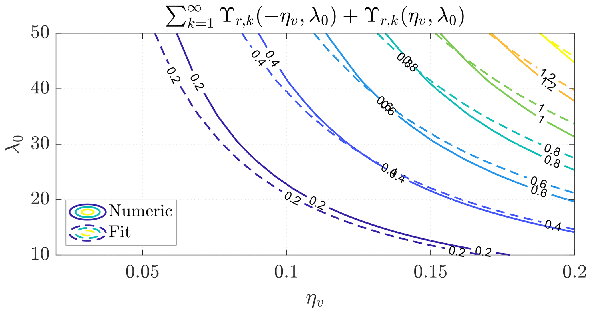
Figure A1 Summation modeling the far-wake radial shape function obtained numerically (solid lines) and the fitted function (dashed lines).

For an elliptic wing, ${\mathit{\eta }}_{\mathrm{v}}=\frac{\mathit{\pi }}{\mathrm{4}}{\mathit{\kappa }}_{\mathrm{0}}$ and ${\mathrm{\Gamma }}_{\mathrm{0}}=\mathrm{2}b\frac{u_{\mathrm{0}}{C}_{\mathrm{L}}}{\mathit{\pi }\mathrm{AR}}$. The radial induction is then

$$\begin{array}{}\text{(A8)}& a_r\approx \mathit{\lambda }{\displaystyle \frac{\mathrm{2}}{\mathrm{9}\mathit{\pi }}}{\displaystyle \frac{C_{\mathrm{L}}}{\mathit{\pi }\mathrm{AR}}}{\mathit{\kappa }}_{\mathrm{0}}^{\mathit{\pi }/\mathrm{2}}{\mathit{\lambda }}_{\mathrm{0}}^{\mathrm{1.1}}.\end{array}$$

Appendix B: Comparison of glide ratios

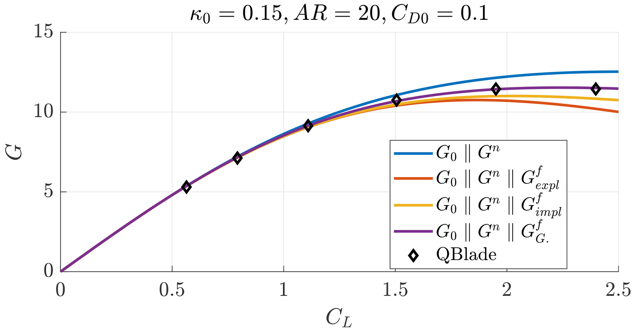
Figure B1 Glide ratio as a function of the lift coefficient for a case with AR=20, κ₀=0.15 and C_D0=0.1.

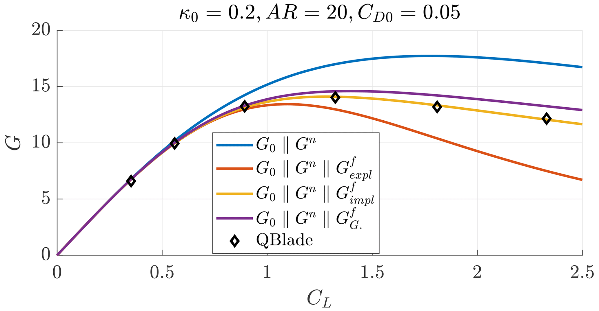
Figure B2 Glide ratio as a function of the lift coefficient for a case with AR=20, κ₀=0.2 and C_D0=0.05.

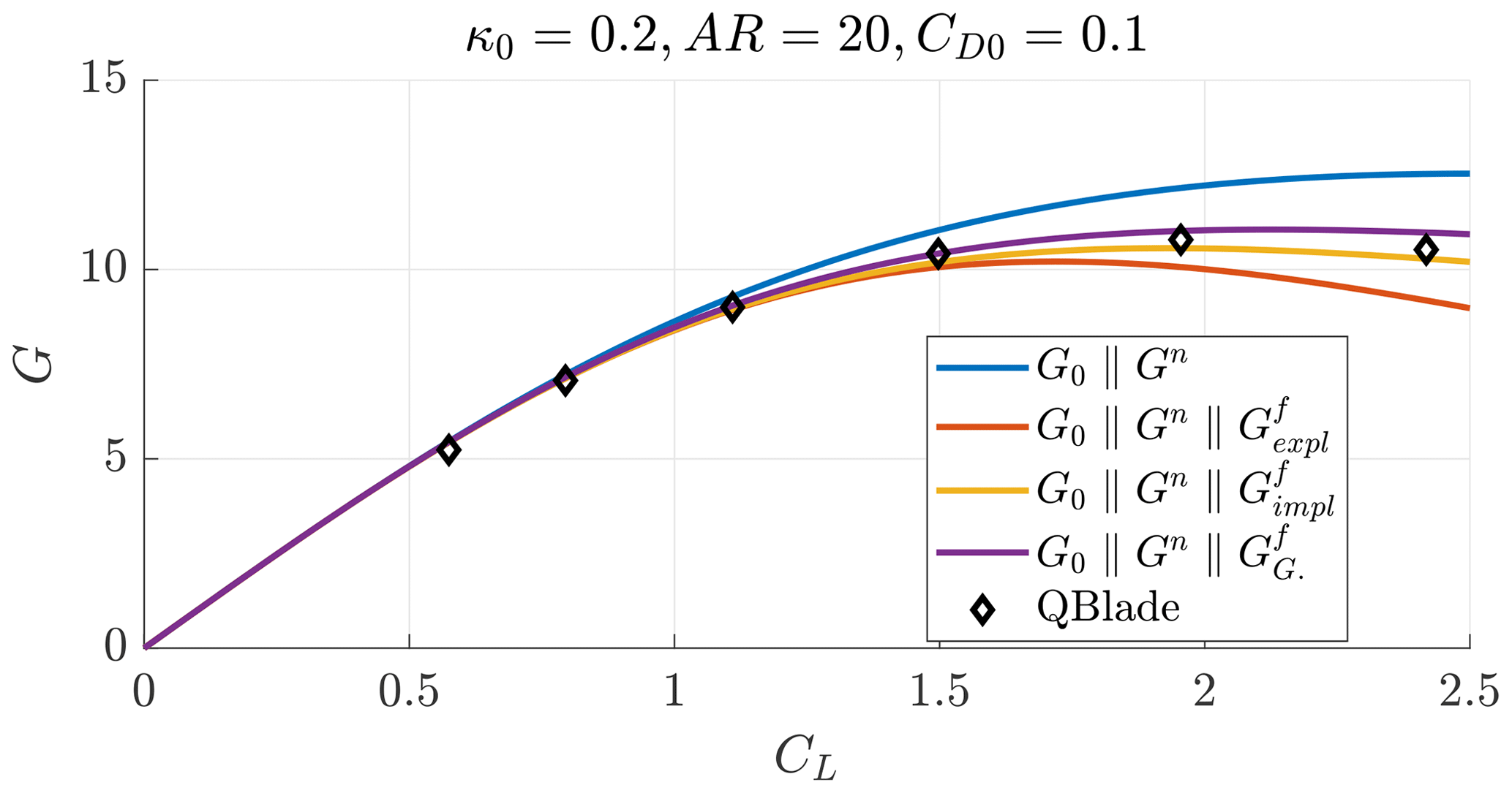
Figure B3 Glide ratio as a function of the lift coefficient for a case with AR=20, κ₀=0.2 and C_D0=0.1.

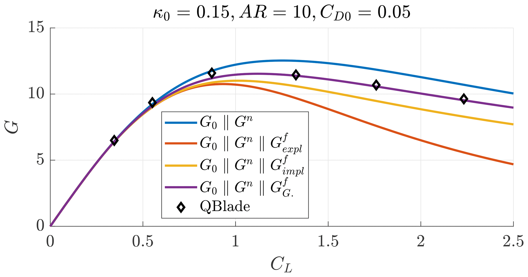
Figure B4 Glide ratio as a function of the lift coefficient for a case with AR=10, κ₀=0.15 and C_D0=0.05.

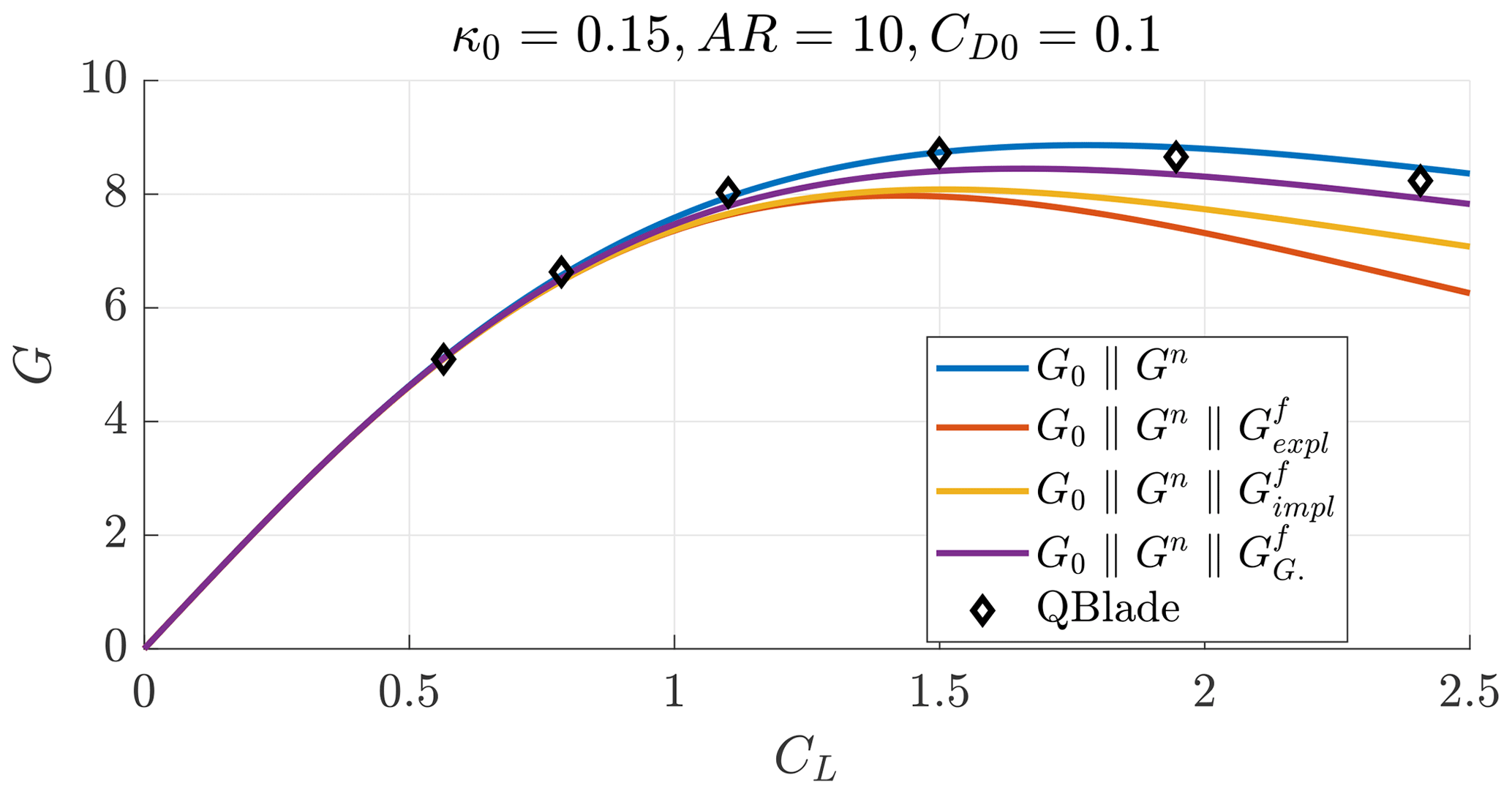
Figure B5 Glide ratio as a function of the lift coefficient for a case with AR=10, κ₀=0.15 and C_D0=0.1.

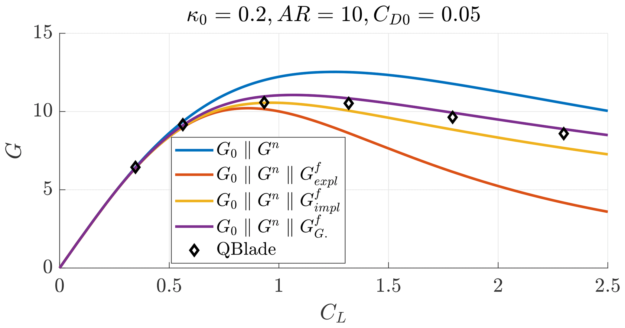
Figure B6 Glide ratio as a function of the lift coefficient for a case with AR=10, κ₀=0.2 and C_D0=0.05.

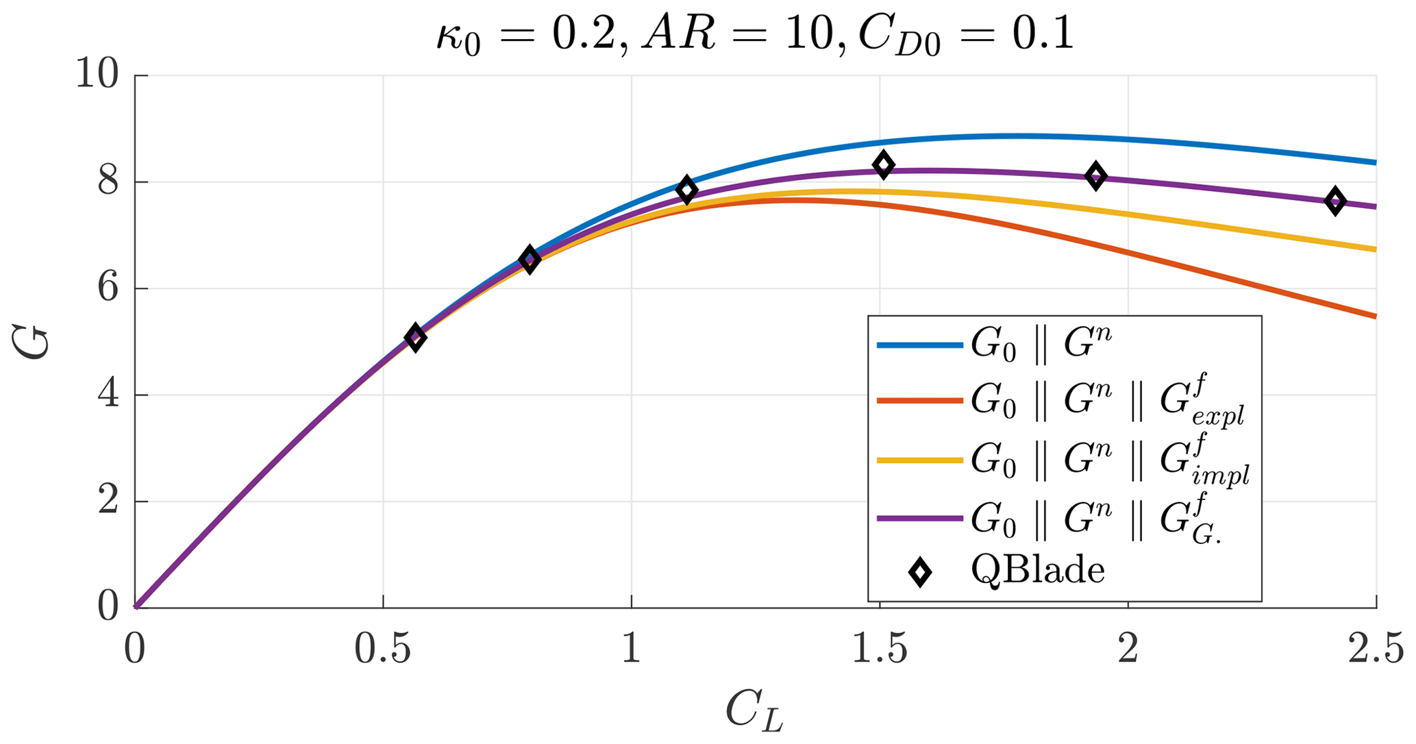
Figure B7 Glide ratio as a function of the lift coefficient for a case with AR=10, κ₀=0.2 and C_D0=0.1.

Appendix C: Nomenclature

Latin symbols
A	Wing area
ar	Radial induction
az	Axial induction
AR	Wing aspect ratio
b	Wing span
CD	System drag coefficient
CD0	System drag coefficient at zero lift
CDi	Induced drag coefficient
CL	Wing lift coefficient
G	$C_{\mathrm{L}}/C_{\mathrm{D}}$: glide ratio

Latin symbols
G0	$C_{\mathrm{L}}/C_{\mathrm{D}\mathrm{0}}$: glide ratio related to the drag
	coefficient at zero lift
Gf	$C_{\mathrm{L}}/C_{\mathrm{Di}}^{\mathrm{f}}$: glide ratio related to the far-
	wake drag coefficient
Gn	$C_{\mathrm{L}}/C_{\mathrm{Di}}^{\mathrm{n}}$: glide ratio related to the near-
	wake drag coefficient
h0	Helicoidal wake pitch
pj	Evaluation point
R0	Mid-span turning radius
Rf	Radius of the helicoidal vortex filament
Rj	Evaluation point radius
u0	AWES longitudinal velocity
v0	Radial induced velocity at the wing
	center
vo	Reel-out velocity
vr	Relative wind speed
vw	Wind speed
w	Axial induced velocity
w0	Axial induced velocity at the wing
	center
yf	Rf−R0: vortex filament spanwise
	position
yj	Rj−R0: evaluation point spanwise
	position
Greek symbols
αi	Induced change in the angle of attack
ΔR	Rj−Rf
η	$\mathrm{\Delta }R/R_j$
η0	$-y_{\mathrm{f}}/R_{\mathrm{0}}$
ηj	$y_j/R_{\mathrm{0}}$
Γ	Bound vorticity
γ	Trailed vorticity
Γ0	Intensity of the rolled-up trailed
	vortices
κ0	$b/\left(\mathrm{2}{R}_{\mathrm{0}}\right)$: inverse turning ratio
λ	$u_{\mathrm{0}}/v_{\mathrm{r}}$: wing speed ratio
λ0	Normalized torsional parameter of the
	helicoidal wake
ϕj	Angular position of the evaluation point
	pj around e1 starting from e2
ρ	Air density
θ	Angular parameter of the helix
θj	Angular position of the evaluation point
	pj around e3 starting from e2
Υn	Shape factor modeling the near-wake
	axial induction
${\mathrm{{\rm Y}}}_{z,k}^{\mathrm{f}}$	Shape factor modeling the axial
	induction produced by the kth vortex
	ring
Υr,k	Shape factor modeling the radial
	induction produced by the kth vortex
	ring