the Creative Commons Attribution 4.0 License.
the Creative Commons Attribution 4.0 License.
 | 08 Jan 2024
A digital twin solution for floating offshore wind turbines validated using a full-scale prototype
Emmanuel Branlard
Jason Jonkman
Cameron Brown
Jiatian Zhang
In this work, we implement, verify, and validate a physics-based digital twin solution applied to a floating offshore wind turbine. The digital twin is validated using measurement data from the full-scale TetraSpar prototype. We focus on the estimation of the aerodynamic loads, wind speed, and section loads along the tower, with the aim of estimating the fatigue lifetime of the tower. Our digital twin solution integrates (1) a Kalman filter to estimate the structural states based on a linear model of the structure and measurements from the turbine, (2) an aerodynamic estimator, and (3) a physics-based virtual sensing procedure to obtain the loads along the tower. The digital twin relies on a set of measurements that are expected to be available on any existing wind turbine (power, pitch, rotor speed, and tower acceleration) and motion sensors that are likely to be standard measurements for a floating platform (inclinometers and GPS sensors). We explore two different pathways to obtain physics-based models: a suite of dedicated Python tools implemented as part of this work and the OpenFAST linearization feature. In our final version of the digital twin, we use components from both approaches. We perform different numerical experiments to verify the individual models of the digital twin. In this simulation realm, we obtain estimated damage equivalent loads of the tower fore–aft bending moment with an accuracy of approximately 5 % to 10 %. When comparing the digital twin estimations with the measurements from the TetraSpar prototype, the errors increased to 10 %–15 % on average. Overall, the accuracy of the results is promising and demonstrates the possibility of using digital twin solutions to estimate fatigue loads on floating offshore wind turbines. A natural continuation of this work would be to implement the monitoring and diagnostics aspect of the digital twin to inform operation and maintenance decisions. The digital twin solution is provided with examples as part of an open-source repository.
- Article
(8362 KB) - Full-text XML
- BibTeX
- EndNote


This work was authored in part by the National Renewable Energy Laboratory, operated by Alliance for Sustainable Energy, LLC, for the US Department of Energy (DOE) under contract no. DE-AC36-08GO28308. The US Government retains and the publisher, by accepting the article for publication, acknowledges that the US Government retains a nonexclusive, paid-up, irrevocable, worldwide license to publish or reproduce the published form of this work, or allow others to do so, for US Government purposes.
The offshore floating wind turbine market is expected to grow in the coming decades as the technology gains in maturity, with several floating wind turbine prototypes already tested and commissioned, such as the TetraSpar, developed by Stiesdal Offshore (Stiesdal Offshore, 2022). Operation and maintenance (O&M) costs can account for approximately one-third of offshore wind farm life cycle expenditures for a fixed-bottom project and are expected to be higher for remote (floating) projects (Castella, 2020). Reducing the O&M costs is therefore an impactful and effective means to lower the costs of floating offshore projects. Digital twin solutions are increasingly being used to follow products during their life cycle to assess component conditions, guide predictive maintenance, and thereby reduce O&M costs. A review of digital twins for power systems is found in Song et al. (2023). Digital twins often include a virtual sensing component that provides information not measured by the physical system and a structural health monitoring component to assess the condition of the system. Virtual sensing technology is usually achieved using physics-based or data-driven approaches, with both approaches relying on measurements from the physical system to infer and extrapolate information about its current state. Physics-based approaches use a numerical model of the system, whereas data-driven approaches use either ad hoc algorithms or machine-learning techniques. Machine-learning approaches can be trained using high-fidelity models or measurements, leading to potentially high accuracies while maintaining low computational time, but their training requirements imply that a technology cannot be readily transferred from one platform to another. Physics-based models often require low-fidelity models to achieve computational times low enough for digital twins to run in real time. They nevertheless offer the advantage that they provide tractable and insightful results, and they can be applied to a same family of wind turbine concepts because they do not require a training dataset. Currently, there is no definite case as to which approach can lead to the best digital twin implementation, and it is possible that future approaches will combine physics-based with data-driven techniques. This work presents the development, verification, and validation of a physics-based digital twin for floating wind turbines as a proof of concept for future maturation of the technology.
Digital twins for wind turbine applications have recently become a topic of research interest. The authors explored the topic of physics-based digital twins in previous work, in which a method to estimate tower loads on land-based turbines was developed (Branlard et al., 2020a, b). The approach relied on a Kalman filter model (Kalman, 1960; Zarchan and Musoff, 2015) that combines a linear physics-based model of the structure with measurements from the turbine to perform a virtual sensing of the tower section loads and estimate the fatigue of this component. The measurement data were taken from the supervisory control and data acquisition (SCADA) system using sensors readily available on most turbines. The approach used a mix between an augmented Kalman filter approach (Lourens et al., 2012), where the loads are estimated with the states of the system, and a physics-based aerodynamic estimator for aerodynamic thrust. Bilbao et al. (2022) used a Gaussian process latent force model to estimate the forcing of the system and thereby obtain the section loads along the tower. Drivetrains are another component for which a digital twin has been applied, with physics-based approaches presented in Mehlan et al. (2022, 2023) and data-driven models presented in Kamel et al. (2023).
Despite the recent popularity of the term “digital twin”, the concept is heavily based on the fields of structural health monitoring and load estimations (or, more generally, virtual sensing), which have long been topics of research. For instance, Iliopoulos et al. (2016) used physics-based modal decomposition to estimate the dynamic response on the substructure of a fixed-bottom wind turbine. Neural networks have been used to establish transfer functions or surrogate models based on SCADA data to obtain wind turbine loads with the aim of performing conditional monitoring (see, e.g., Cosack, 2010; Schröder et al., 2018). Kalman filters were introduced in fields other than wind energy to perform load estimation (Auger et al., 2013; Ma and Ho, 2004; Eftekhar Azam et al., 2015; Lourens et al., 2012). Kalman filtering has been extensively used in wind energy to estimate rotor loads and improve wind turbine control (Boukhezzar and Siguerdidjane, 2011; Selvam et al., 2009; Bottasso and Croce, 2009; Bossanyi, 2003). Load estimations were also achieved using hybrid techniques combining physics based on SCADA data by Noppe et al. (2016). Other load estimation techniques may be used, such as lookup tables (Mendez Reyes et al., 2019), modal expansion (Iliopoulos et al., 2016), machine learning (Evans et al., 2018), neural networks (Schröder et al., 2018), polynomial chaos expansion (Dimitrov et al., 2018), deconvolution (Jacquelin et al., 2003), or load extrapolation (Ziegler et al., 2017).
In this work, we build on our previous work related to fixed-bottom turbines and present a digital twin solution for floating wind turbines that relies on physics-based models and a Kalman filter. We apply the digital twin to the TetraSpar structure and use measurements from the full-scale prototype. Achieving computational efficiency is crucial to be able to run the digital twin online; therefore, a reduced-order model with few selected degrees of freedom is used. Developing digital twins for floating wind turbines presents a set of challenges compared to our previous work on fixed-bottom foundations. The potentially large motions undergone by the platform may affect the aerodynamics and accelerometer signals. The models developed for fixed-bottom foundations need to be augmented to be able to predict the aerodynamics when the platform experiences large pitching motions. The dynamics of the platform motion needs to be well captured for the tower-top accelerometer to be used and for estimating the loading in the station-keeping system. In both floating and fixed-bottom wind turbines, hydrodynamic loads need to be estimated to capture member-level loads in the substructure, but they can be omitted as a first approximation if only the tower loads are estimated, as in this study.
In Sect. 2, we provide an overview of our digital concept, the vision for future application, and the TetraSpar prototype on which the digital twin is applied. In Sect. 3, we present the individual components of the digital twin and run some isolated verification studies on them. In Sect. 4, we present results from the digital twin application first using numerical experiments and then using measurements from the TetraSpar prototype before concluding. To avoid lengthening the main text, we provide derivations (some of which are important contributions of this work) and additional results in appendices.
In this section, we provide an overview of our digital twin concept and how it is applied in this study.
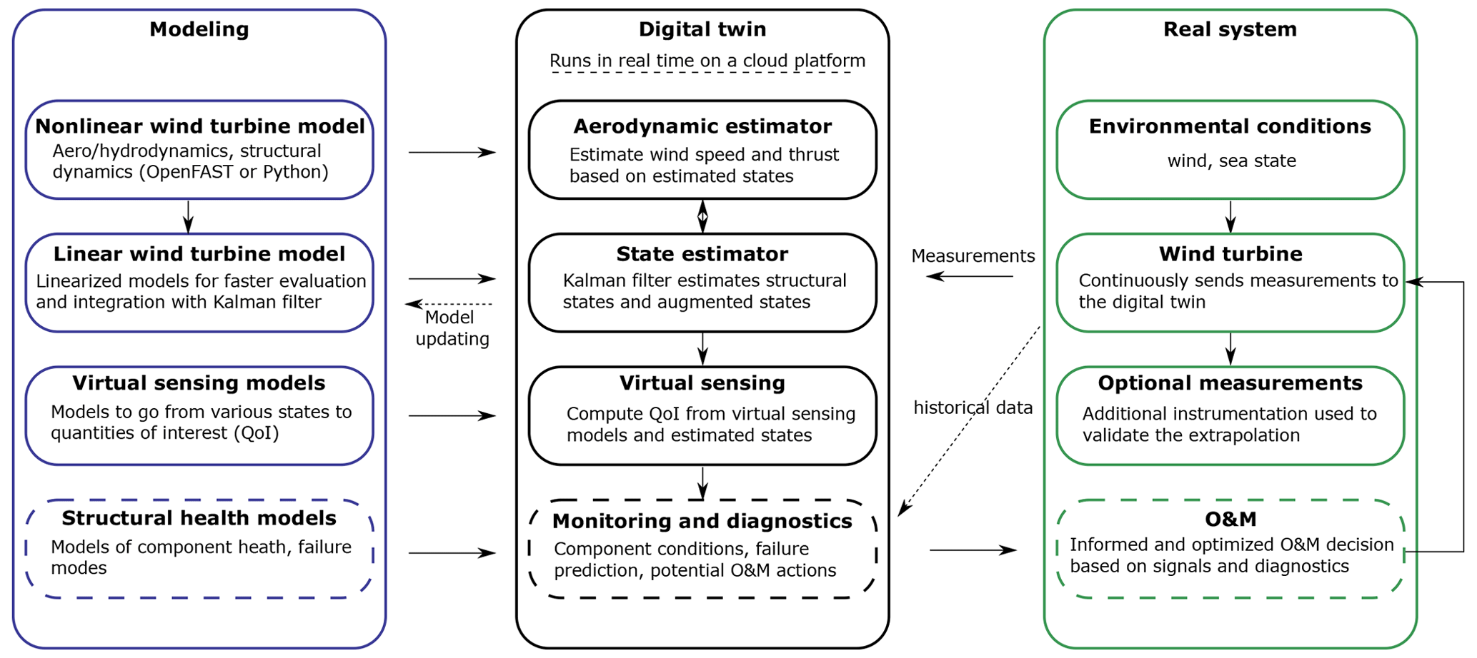
Figure 1Overview of the digital twin concept. Dashed lines indicate features that are outside the current scope.
2.1 Long-term vision of the digital twin concept
Many definitions and applications of digital twins are possible. The vision for the concept discussed in this work is to follow the life cycle of a wind turbine in real time and ultimately provide tangible signals to inform O&M decisions. Our goal is to achieve this by relying only on measurements expected to be available on most wind turbines, thereby avoiding the extra cost of adding sensors. In this work, we leave open the question as to whether the installation of an additional set of optimally placed and selected sensors can further improve the predictions of the digital twin, further reducing the long-term O&M costs, and thereby warranting the additional costs of adding the sensors.
We illustrate our approach and vision in Fig. 1.
The digital twin is intended to run in real time on a cloud platform. It combines a set of models (on the left of the figure) with data from the real system (on the right) to perform the estimation of various states and eventually produce diagnostics that can be used to inform the O&M. The data from the real system are taken from high-frequency measurements from the SCADA system (e.g., power, pitch, rotor speed). The states estimated by the digital twin include aerodynamic states (wind speed, thrust) and motions of the structure (e.g., surge, pitch, tower deflection). The core algorithm in the estimation is a Kalman filter that uses a linear wind turbine model. The estimated states are used in a virtual sensing step to produce quantities of interests (QoIs), such as the loads at key locations of the structure. The QoIs are then intended to be postprocessed by a monitoring and diagnostic tool to generate the data needed to perform condition-based O&M.
2.2 Narrowed scope
The boxes in Fig. 1 with dashed-line borders – structural health modeling, monitoring and diagnostics, and O&M decisions – are postponed to future work, even though they are essential steps to achieve our final vision. Dashed lines and arrows indicate options that may be exploited in the future but are also outside of our scope: the use of historical data to assist in the diagnostics, the use of estimates to perform model updating, and real-time implementation.
This work therefore focuses on the estimation of states and environmental conditions under the assumption that the estimated quantities can replace costly measurements and eventually be used for O&M decisions. We intend to provide a proof of concept that paves the way for future commercial applications. A detailed description of each of the boxes surrounded with solid lines is given in Sect. 3.
2.3 System studied
2.3.1 The TetraSpar prototype
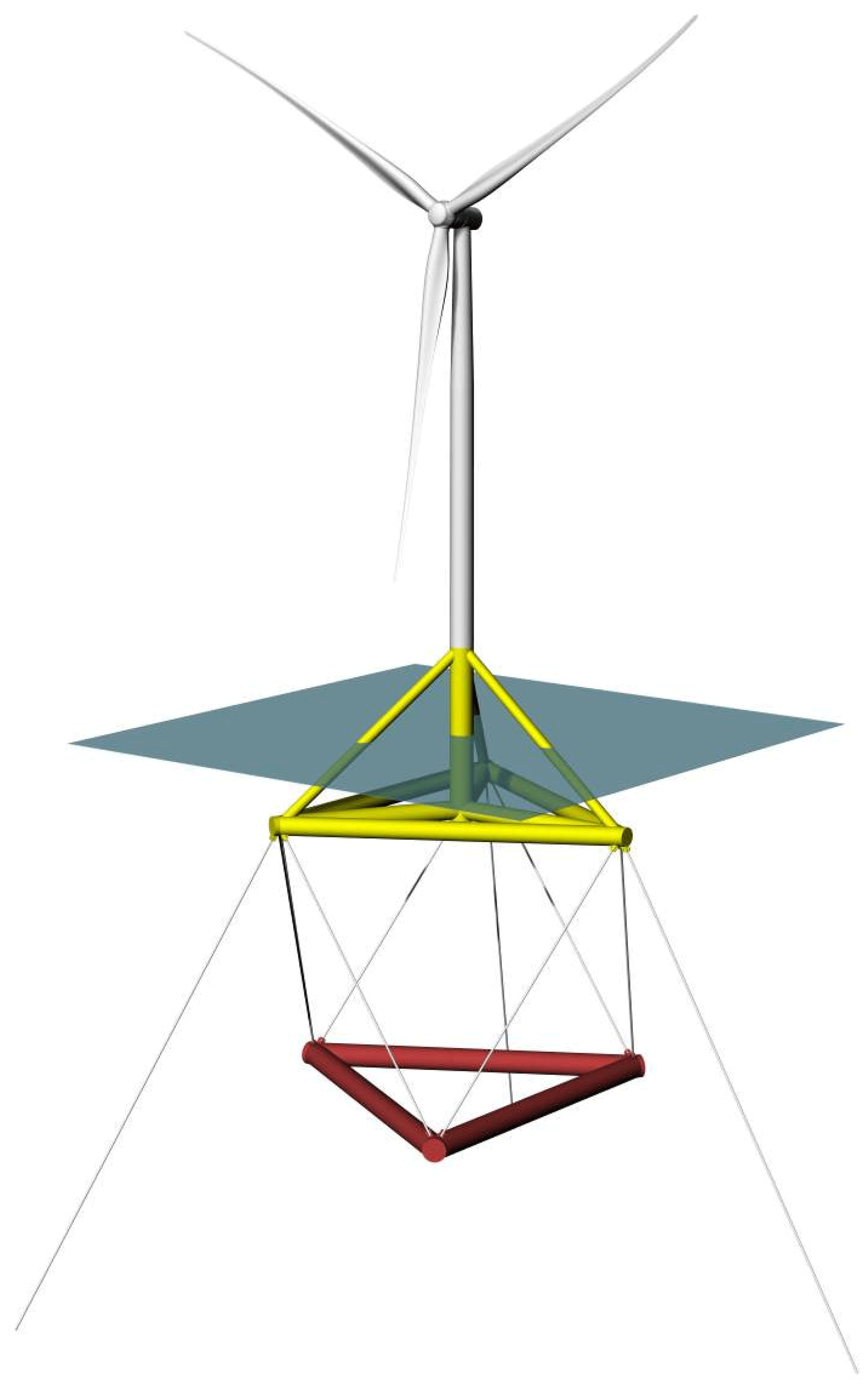
The system studied for this article is the TetraSpar floating offshore prototype. The system consists of a floating platform and station-keeping system developed by Stiesdal Offshore in collaboration with partners Shell, RWE, and TEPCO Renewable Power, as well as a 3.6 MW wind turbine with a rotor diameter of 130 m developed by Siemens Gamesa Renewable Energy. A sketch of the system is provided in Fig. 2.
The prototype was installed off the coast of Norway and commissioned in November 2021. The prototype turbine is equipped with additional sensors (labeled “Optional measurements” in Fig. 1), which we use to validate the estimated QoIs.
2.3.2 Numerical experiments
Prior to using measurement data, we use simulations (referred to as “numerical experiments”) in place of the real system to feed data to the digital twin. The advantage of this approach is that the QoIs are directly accessible and can be compared to the estimates for verification purposes.
Data for the numerical experiments are obtained using OpenFAST simulations (Jonkman et al., 2023a, b). A model of the TetraSpar floating platform and the wind turbine was implemented in OpenFAST based on data provided by the manufacturers. All the members of the substructure are modeled using the strip-theory approach (Morison equation) because the inherent long-wavelength assumption of the strip theory has been shown to be sufficiently accurate for this structure with relatively slender members. The OpenFAST model is complemented with NREL's Reference OpenSource Controller (ROSCO, Abbas et al., 2022). The controller parameters are tuned so that OpenFAST simulations match the operating conditions of the turbine extracted from SCADA data (pitch, rotor speed, and power). The nacelle velocity feedback option of ROSCO is used to reduce the platform pitching motion. Using trial and error, the frequency and damping ratio of the pitch PI controller are set to ωp=0.05 rad s−1 and ζp=7 %, and the values for the torque controller are set ωQ=0.15 rad s−1 and ζQ=7 %. The gain scheduling of the pitch controller is obtained using the tuning feature of ROSCO. We note that the controller is only needed to perform verifications of the digital twin with realistic time series of the turbine responses, but the controller itself is not used for the design of the digital twin. We use the following modules of OpenFAST (Jonkman et al., 2023a, b): MAP (mooring lines), HydroDyn (hydrodynamics), ElastoDyn (tower and blade elasticity; rigid floater), AeroDyn (aerodynamics), InflowWind (wind inflow), and ServoDyn (controller interface).
For the numerical experiments, we use synthetic turbulent wind fields generated using TurbSim (Jonkman and Buhl, 2006). In particular, we often use the same wind field, which we refer to as the “turbulent step”, where a deterministic ramp and drop are added to a turbulent field. The advantage of this 10 min wind field is that it covers all the operating regions of the turbine in a challenging way because the variations of the wind speed are sudden. The wind speed at hub height for the turbulent step can be seen in Fig. 6.
2.3.3 Main aspects of the structural model
We model the structure using a set of 8 degrees of freedom (DOFs), as illustrated in Fig. 3.
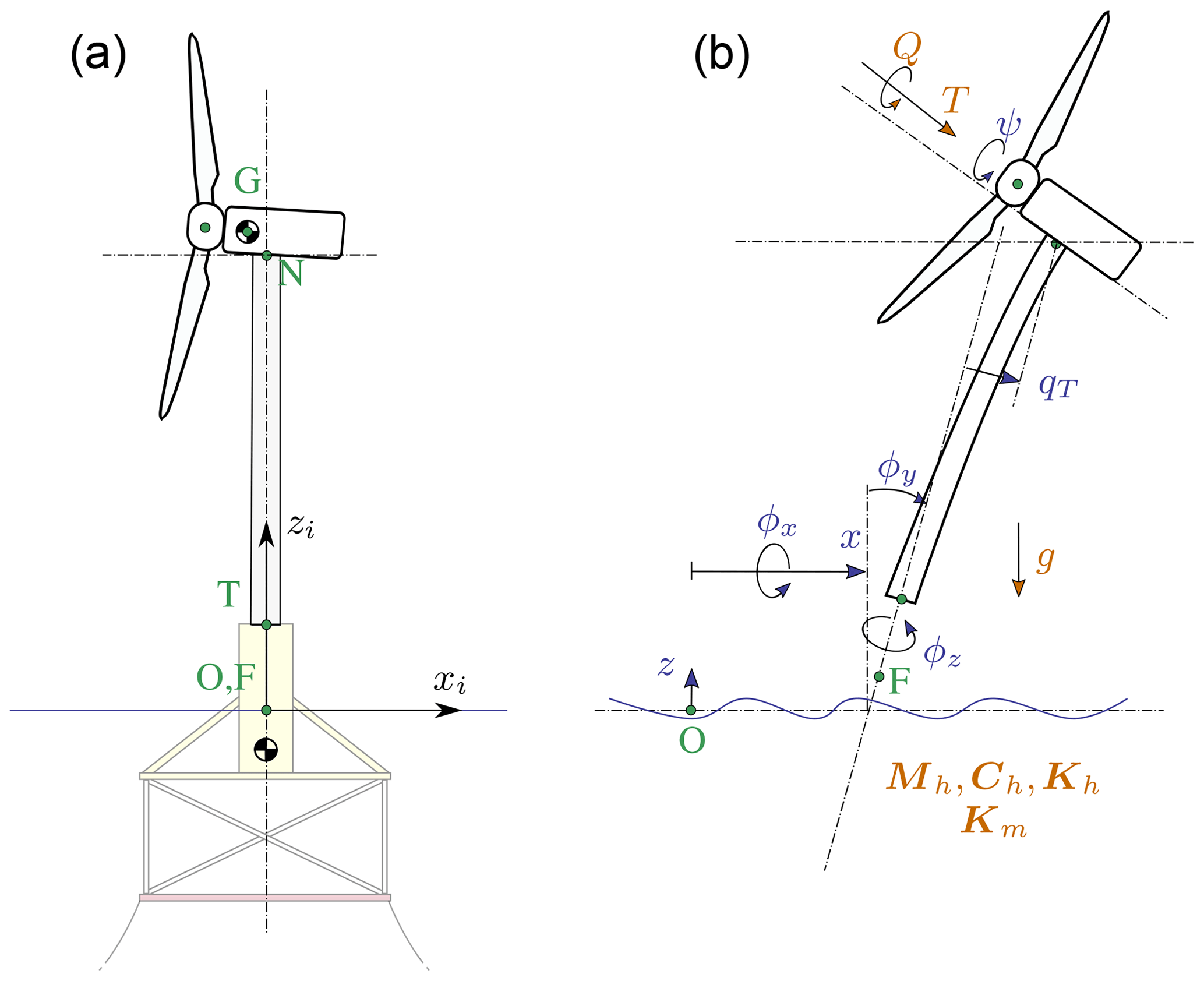
Figure 3Notations for the structural modeling of the floating wind turbine, assuming no yawing of the nacelle. (a) Main points () and inertial coordinate system (i). (b) Degrees of freedom () and main loads: aerodynamics (T,Q), hydrodynamics (6×6 mass and damping and stiffness matrices, Mh, Ch, Kh; wave-excitation force neglected), mooring (6×6 stiffness matrix, Km), and gravity (g).
The platform is represented as a rigid body, and its motion is described using 6 DOFs: surge, sway, heave, roll, pitch, and yaw, respectively noted , and ϕz. The tower bending in the fore–aft direction is represented using 1 generalized DOF, qt, associated with a Rayleigh–Ritz shape function, taken as the first fore–aft mode shape of the tower (Branlard, 2019). The side–side tower bending can be added in a similar way, but for simplicity, it was not considered in this study. The shape function along the tower height, zt, is written as Φ(zt), with Φ(0)=0 at the tower bottom and Φ(LT)=1 at the tower top, where LT is the tower length. The shaft rotation is noted ψ, so that the rotation speed of the rotor is , where the dot notation indicates differentiation with respect to time. The rotor–nacelle assembly is modeled as a rigid body. The full vector of DOFs is therefore . The equations of motion will be recast into a first-order form by concatenating the vector of DOFs and its time derivative, . The selected set of DOFs captures the first-order effects as it is the minimal set required to capture the full motion of the floater (necessary to compute restoring loads and tower loads), the tower flexibility (necessary to capture tower loads), and the rotor motion (necessary to capture the aerodynamics). Additional degrees of freedom could be considered to increase the modeling accuracy, in particular to include floater flexibility for internal calculation of substructure member loads. This would increase the computational requirement and only contribute to second-order effects, and it is therefore postponed to future work.
In this work, we perform simplifying assumptions, e.g., neglecting the influence of nacelle yaw on the system. The measurement data are conveniently provided in the fore–aft and side–side system of the nacelle. The main assumption is therefore that we assume a rotational symmetry of the platform and mooring system about the yaw axis. We intend to lift this assumption in future work. Some of the consequences of this assumption is that we do no capture changes of inertial properties due to asymmetry of the support structure and changes of stiffness of the mooring system. In the case of the TetraSpar, the mass matrix of the floater does not vary significantly with the yawing of the coordinate system, and the assumption is fair. We note that if the structure had perfect 120∘ symmetry about the yaw axis, then its inertia would be invariant by yaw rotation. For the restoring stiffness of the mooring system, the diagonal terms do not vary significantly as the coordinate system yaws, but some of the coupling terms vary by 50 % to 200 %. The couplings between the platform DOFs are likely wrongly estimated under the rotational symmetry assumption. The impact is nevertheless limited because most of the platform DOFs (, and ϕy) are measured and therefore observable by the Kalman filter.
In this section, we describe and verify the individual components of the digital twin presented in Fig. 1. In Sect. 4, we present applications of the digital twin where all the individual components are combined together.
3.1 Wind turbine measurements
The measurements used as inputs to the digital twin are listed in Table 1.
Table 1Measurements used as inputs to the digital twin.
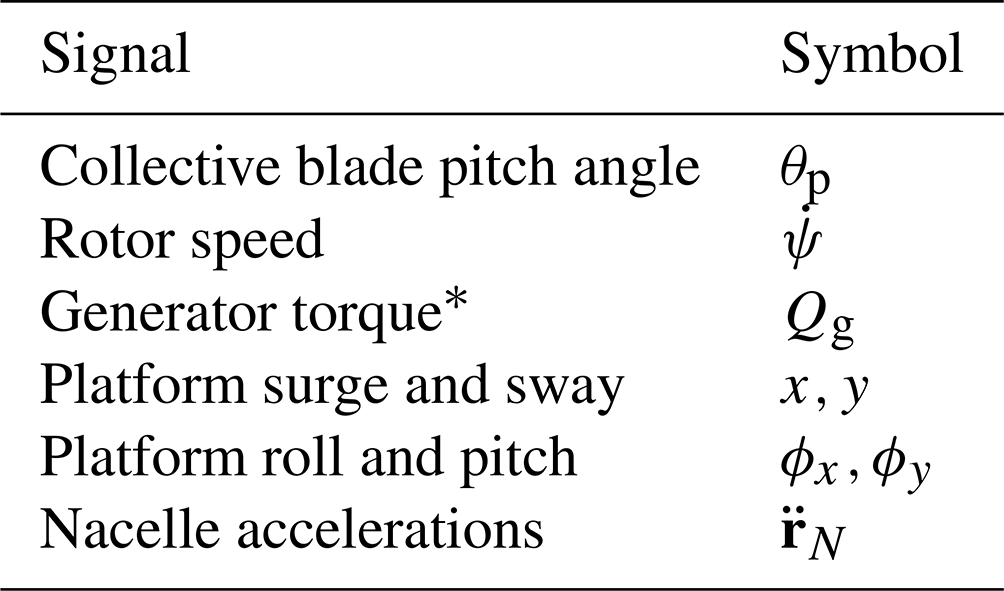
* Obtained from the power measurement using Eq. (2).
These outputs are stored in a database at a sampling rate of 25 Hz. We expect these measurements to be standard sensors for any floating wind turbine. The TetraSpar prototype is equipped with additional measurements that are used to validate the implementation of the digital twin (see Sect. 4).
3.2 Nonlinear wind turbine models
3.2.1 Overview
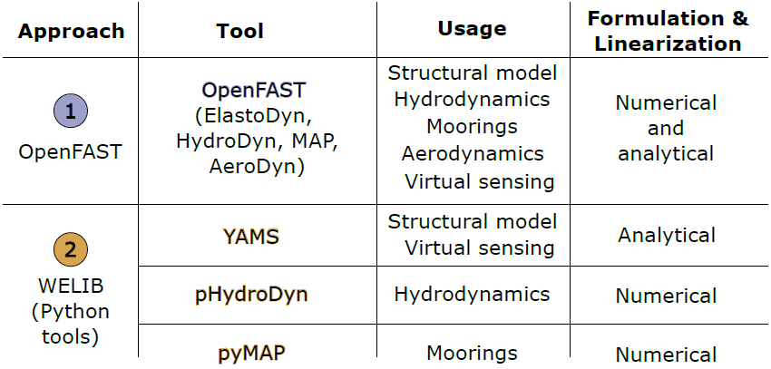
Similar to our previous work (Branlard et al., 2020b), we use two different pathways to obtain nonlinear and linear models of floating wind turbines: OpenFAST and WELIB (Wind Energy LIBrary, Branlard, 2023c, d). The OpenFAST approach was described in Sect. 2.3.2, it is compared to the WELIB approach in Table 2, and the WELIB toolset is further discussed below. In the next sections, we will show that the results from both approaches are consistent with each other so that either of the two can be used to obtain nonlinear and linear reduced-order models. Ultimately, in Sect. 4, a mix of the two approaches is used for the digital twin: linear OpenFAST models for the state-space equations (Sect. 3.5) and WELIB for the virtual sensing step (Sect. 3.6).
3.2.2 WELIB tools
The WELIB approach consists of a set of dedicated open-source Python tools that are similar to the ElastoDyn, HydroDyn, and MAP modules of OpenFAST. We developed these tools to offer additional modularity and granularity: the tools can be called individually or together; their states, inputs, and outputs can be accessed and manipulated at each time step; and the Python scripting eases the manipulation of the models. For instance, this allows for
-
analytical linearization of the structural dynamics,
-
simple linearization of the hydrodynamics (obtention of 6×6 matrices),
-
linearization of hydrodynamics with respect to wave elevation,
-
linearization with respect to parameters (Jonkman et al., 2022), and
-
interactive time stepping of the linear and nonlinear model.
In this work, we mostly use the first two features listed above, and their usage will be described in Sect. 3.3.2. Results from time-stepping simulations will be presented in Sect. 3.3.3. We expect to exploit the additional features of WELIB in future digital twin implementations. For this work, we implemented the following tools in WELIB: (1) YAMS, a symbolic structural dynamics package to obtain the equations of motion of an assembly of rigid and flexible bodies analytically and allow for their analytical linearization (Branlard and Geisler, 2022); (2) pHydroDyn, a Python version of the module HydroDyn (with a subset of HydroDyn's functionality) to determine the hydrodynamic loads; and (3) pyMAP, a wrapper around the MAP module of OpenFAST to obtain the mooring quasi-statics. With these three additions, it is possible to perform nonlinear simulations of floating wind turbines using WELIB and perform comparisons with OpenFAST.
3.2.3 Differences between the two nonlinear approaches
Currently, no controller or aerodynamic module is present in WELIB. Therefore, nonlinear time-stepping simulations with WELIB are limited to free-decay simulations or prescribed loads. Another shortcoming is that WELIB does not cover the full range of options available with OpenFAST, which is a continuously evolving, extensively verified and validated tool. Such options include the potential flow representation of hydrodynamic bodies, the flexibility of the floating structure, and aerodynamic and control features. One benefit of WELIB over OpenFAST is the possibility to perform interactive time stepping, that is, to change the states and inputs dynamically during the simulation. We do not use this approach in this work, but it can be considered for nonlinear digital twin applications, for instance, using an extended Kalman filter algorithm. Another benefit is the possibility to obtain analytical linear models of the structure, which avoids using finite differences and therefore reduces the associated numerical errors. In the WELIB approach, the individual modules are linearized separately before being combined into the final linear model, and it is therefore easier to understand where each term in the Jacobians of the linear models comes from and thereby gain physical intuitiveness on the model. Ultimately, the linear models obtained by both approaches are similar and differ mostly based on differences in the structural dynamics equations and the implementation of rotational transformation matrices. Results comparing time simulations using both approaches will be presented in Sect. 3.3.
3.3 Linear wind turbine models
As part of our digital twin concept, we have chosen to use linear wind turbine models and a Kalman filter for the core of the state estimation (see Sect. 3.5). Nonlinear models and an extended Kalman filter could be considered in future iterations. In this section, we describe how the linear models from OpenFAST and WELIB are obtained.
3.3.1 OpenFAST linearization
OpenFAST can provide full-system linearization of its underlying nonlinear models by using a mix of analytically and finite-difference-derived Jacobians (Jonkman and Jonkman, 2016; Jonkman et al., 2018). The linearization process provides the state-space model () and output equation () for small perturbations (indicated with δ) of the internal states (x), inputs (u), and outputs (y) of OpenFAST, around a selected operating point. OpenFAST provides the linear model for the entire set of states, inputs, and outputs present in the model (including virtual sensor-type outputs typically written to an output file and not used internally). In this work, we extract subsets of the A, B, C, and D matrices and combine them to form the linear model of the state estimator (see Sect. 3.5).
3.3.2 WELIB linearization
WELIB performs the linearization of the structure, hydrodynamics, and moorings independently before combining them into one model. The aerodynamic loads are not linearized because a dedicated aerodynamic estimator is used in this work (see Sect. 3.4). The steps are as follows.
-
The structural equations are linearized analytically using our symbolic framework (Branlard and Geisler, 2022). We introduced a notion of “augmented inputs” to linearize the equations of motion without explicit knowledge of the external forces. The process is described in Sect. A.
-
We compute the 6×6 linearized rigid-body hydrodynamics matrices (mass matrix Mh, damping matrix Ch, and stiffness matrix Kh) corresponding to the six rigid-body motions of the platform. At the time of this study, these matrices could not be obtained directly from OpenFAST. While working on this issue, we ended up devising multiple ways to obtain them. They can now be obtained using (1) full-system linearization of the HydroDyn module, (2) the Python implementation of the HydroDyn module by performing rigid-body perturbations of the full platform, or (3) an upgraded version of the OpenFAST HydroDyn driver that also uses rigid-body perturbations. The first approach uses baseline OpenFAST functionalities but requires additional postprocessing scripts and derivations. The full-system linearization of OpenFAST provides Jacobians of the hydrodynamic loads as a function of motions of the individual hydrodynamic analysis nodes (of which models often have hundreds to thousands of). To transfer these individual Jacobians to the reference point and obtain the 6×6 matrices, we developed and used the method presented in Sect. B. The process is involved and prone to errors. In comparison, the second and third approaches are straightforward to implement and are several orders of magnitude faster. The Python version was implemented first and then ported over to Fortran so that it can be readily available to the OpenFAST community. The consistency between the different approaches was verified, and because of its ease of use, the second approach is retained in this study. We note that in this study, all members are modeled using the Morison equation and the hydrodynamic drag is set to zero during the linearization process. There is therefore no frequency-dependent damping, and the effect of hydrodynamic drag is assumed to be part of the modeling uncertainty of the state estimator (see Sect. 3.5).
-
The linearized 6×6 mooring stiffness matrix, Km, is obtained by calling the linearization feature of the MAP module and transferring the Jacobian to the reference point using the method outlined in Sect. B.
-
The linearized equations of motion are assembled as
where the matrices with subscript 0 originate from the linearization of the structure (see Sect. A). The matrix Q0, of dimension 8×6, maps the subset of the 6 rigid-body platform DOFs (), used for the definitions of Mh, Ch, Kh, and Km, to the full vector of DOFs, q. The term δfa is an approximation of the aerodynamic loads and will be discussed in Sect. 3.4. The term δfh is an approximation of the hydrodynamic wave-excitation loads. In this work, δfh is mapped into the inherent model noise of the Kalman filter (see Sect. 3.5). Assuming that the loading is part of the model noise is a crude approximation that is expected to be fair as long as the loading has a zero mean value, which is expected to be the case for the wave loading but not for the wind or current loading (here omitted). This modeling choice is not very influential in this work because the motions of the platform measured by the inclinometers and GPS sensors inherently carry information about the wave loading. Improvements could be obtained by including a model for the wave-excitation loads and further limiting the wave load signal such that it remains within a certain frequency band.
For instance, we could introduce a hydrodynamic state analog to the wave elevation or a set of states that scales different hydrodynamic shape functions so that the hydrodynamic load can be obtained as a linear superposition of scaled shape functions. In our application (tower section loads), such modeling did not appear necessary, but it will be considered in future work as it can be relevant to estimate substructure loads.
-
We recast Eq. (1) into a first-order system to obtain the state matrix A.
3.3.3 Verification of the linear models
In this section, we compare results from the OpenFAST nonlinear model, the OpenFAST linear model, and the WELIB linear model for free-decay simulations of the TetraSpar structure. Free-decay simulations are sufficient because wave and aerodynamic loads are purposely not included in the linear models used by the digital twin. The OpenFAST linear model is obtained about the operating point defined by q0=0 and rpm. All models (including the OpenFAST nonlinear model) use 8 DOFs. The initial conditions are set to (in m and ∘) and rpm, after which the structure is free to move.
First, simulation without hydrodynamics (structure only) is considered to isolate and verify the structural dynamics part of the models. The time responses from the linear and nonlinear models are in strong agreement when only the structure is considered (see results in Sect. C). Then, we consider results for a model that includes hydrodynamics but without wind or external waves (still water). We set the hydrodynamic drag to zero due to the difficulty in linearizing this term and let the state estimator account for this modeling uncertainty. Results of the free-decay simulation are given in Fig. 4 for a time period of 153 s corresponding to the surge frequency. When hydrodynamics is included, the time responses from the linear models are in strong agreement with the nonlinear OpenFAST results for the surge, heave, pitch, and tower fore–aft DOFs. The sway, roll, and rotor speed responses tend to drift as the simulation time advances, which we assume can be attributed to inherent differences between linear and nonlinear models. The coefficient of determination (R2) is indicated in Fig. 4, comparing the linear models to the reference OpenFAST simulations for each response. In all cases, the OpenFAST linear model is closer to the nonlinear OpenFAST model than the WELIB model. The consistency between the linear and nonlinear OpenFAST model is expected because they are obtained from the same code base. The WELIB linear model had difficulty capturing the yaw response. We believe that some of the error in the yaw signal is due to differences between the formulations of the three-dimensional rotations in OpenFAST and WELIB. The difference in yaw results in a difference of coupling between the DOFs, which can explain the differences observed in the sway, roll, and rotor speed signals.
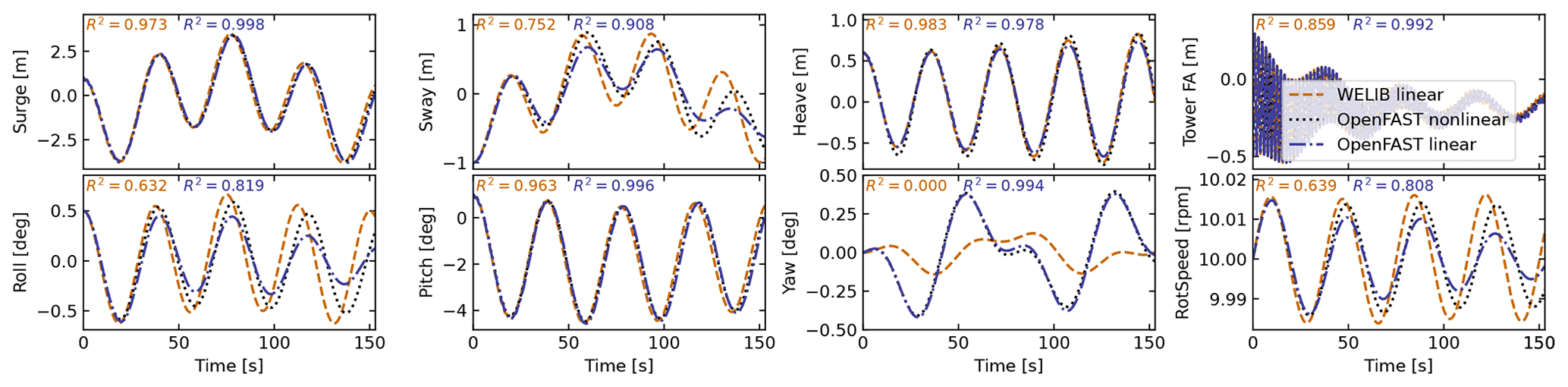
Figure 4Free decay of the structure using nonlinear and linear models for a case including moorings and hydrodynamics (still water). Time series of the main DOFs. RotSpeed stands for rotor speed.
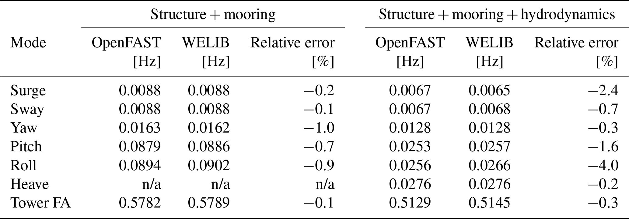
o further quantify the differences between the models, we compare the natural frequencies obtained using the OpenFAST linear and WELIB linear models in Table 3. Overall, the frequencies between the two linear formulations agree very well (less than 2.5 % relative error), except for the roll frequencies (4 % error) with hydrodynamics. Given the results of this section, we will continue this study using the OpenFAST linear model. We expect that continuous development of WELIB will further narrow the gap with OpenFAST in the future.
Table 3Comparison of system frequencies obtained using the WELIB and OpenFAST linear models with and without hydrodynamics (no added mass, damping, hydrostatics, or wave excitation). n/a stands for not applicable.
3.4 Aerodynamic estimator
In Sect. 3.3, we indicated that the linear models were derived without accounting for aerodynamics. Instead, we choose to include the aerodynamic contribution separately within the digital twin. The reason for this choice is that the determination of the aerodynamic loads is essential to capturing the main loading and deflections of the structure, in particular the tower, and the aerodynamic loads vary significantly over the range of operating conditions. Therefore, separating this contribution limits the need to obtain different linearized models for different operating conditions. We have successfully applied this approach in the past (Branlard et al., 2020a). In this work, we extend this approach to accommodate the floating wind application. The different elements of the aerodynamic estimator consist of a torque estimator, aerodynamic maps, and a wind speed estimator.
3.4.1 Kalman filter for torque estimation
We assume that the power and rotor speed are reliable measurement signals, and we further assume that the generator torque (relative to the low-speed shaft) can be inferred from the power signal as
where ηDT is the drivetrain (gearbox and generator) efficiency and n is the gear ratio. For the TetraSpar, n=1, and we assume ηDT=1. The dynamics equation of the drivetrain is modeled as
where JDT is the inertia of the drivetrain about the shaft axis. If we assume that the generator torque is a measurement, then an augmented Kalman filter (Lourens et al., 2012) can be used to estimate the aerodynamic torque Q, using the following state equation:
A random walk approach is used for the evolution of the torque, that is, , and the Kalman filter adds further model noise to this equation. The measurement equation of the Kalman filter is
In the following, we write , the aerodynamic torque obtained using the method outlined above. We present verification results in Sect. 3.4.4.
3.4.2 Aerodynamic maps
It is commonly accepted that the aerodynamic performance of a wind turbine mostly depends on the tip-speed ratio and the pitch angle of the blade. With compliant structures, the bending of the blade, the bending of the tower, and the motions of the floating platform (in particular, the platform pitch) will also affect the aerodynamic performance. These motions are to a large extent a function of the mean wind speed. Therefore, we recommend tabulating the aerodynamic performance as a function of wind speed (U), rotor speed (), blade pitch (θp), and platform pitch (ϕy, assumed to be in the fore–aft direction). The power and thrust coefficients, respectively noted CP and CT, are precomputed using aeroelastic simulations in OpenFAST for a discrete set of values of the four input parameters. In the simulations, the blade and tower elasticity are accounted for. To limit the number of simulations, only the points that are within reasonable proximity of the regular operating conditions of the wind turbine are computed. The 4D aerodynamic maps are precomputed as follows:
The precomputed values are stored in a database.
3.4.3 Wind speed estimation
The digital twin uses the aerodynamic map database to estimate the wind speed and aerodynamic thrust. For a given air density (ρ), rotor radius (R), and measurements , the aerodynamic torque and thrust are readily obtained as a function of wind speed from the database:
where SI units are assumed for all variables. For a given estimated torque (), the estimated wind speed () is found such that
As illustrated in Fig. 5, multiple values of can potentially satisfy Eq. (10) because the aerodynamic torque is a nonlinear function of the wind speed. In such cases, we use the steady-state operating condition curve of the turbine to choose between the multiple solutions (typically two) by selecting the point closest to this curve (see Fig. 5). A relaxation scheme is also used, based on the previous estimate, to alleviate sudden jumps of the estimated wind speed.
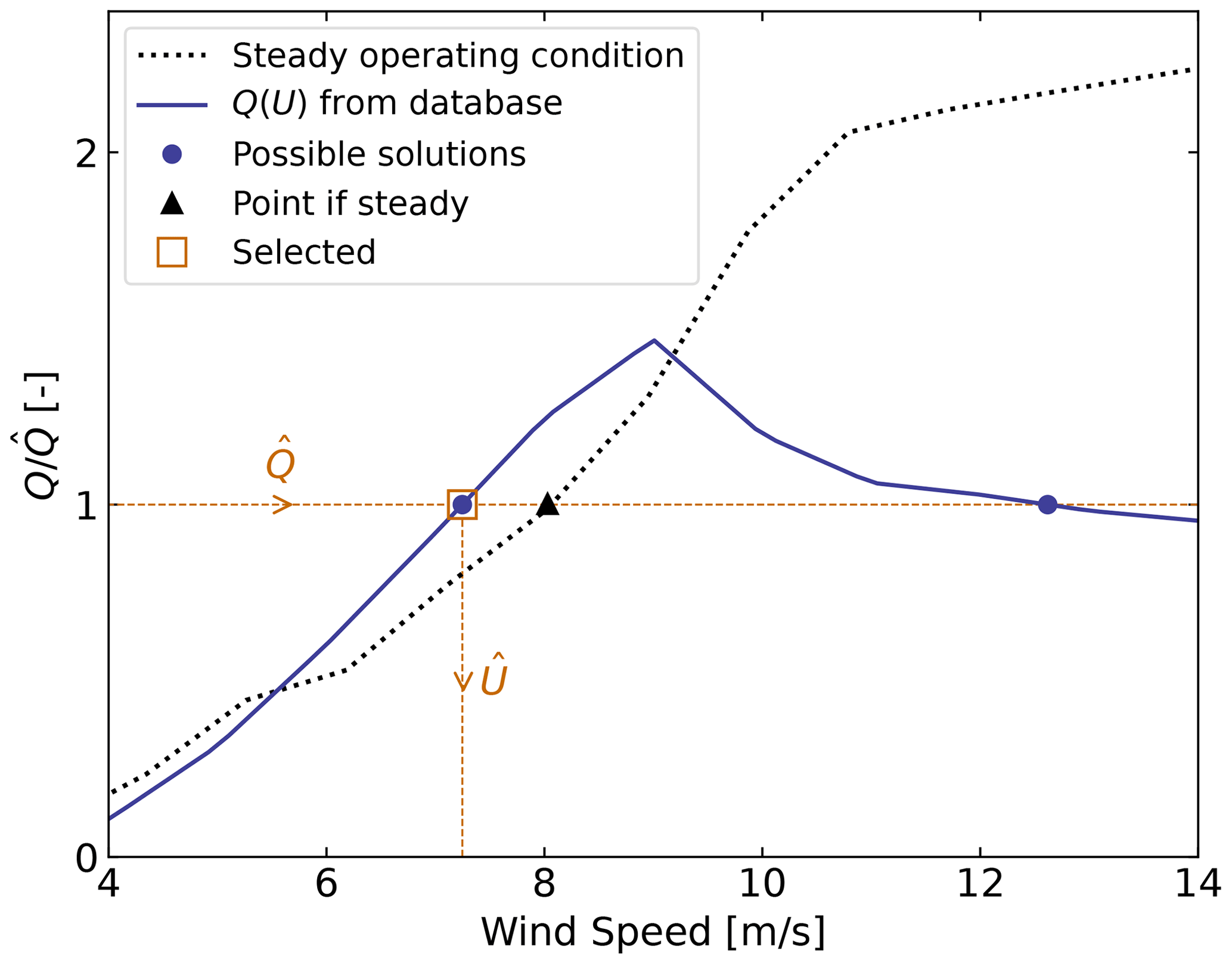
Figure 5Illustration of wind speed estimation in the case where multiple wind speed values match the target torque value .
3.4.4 Verification of the aerodynamic estimator
To verify the aerodynamic estimator, we ran an OpenFAST simulation of the TetraSpar with the turbulent step wind field mentioned in Sect. 2.3.2 and irregular waves computed with a significant wave height of Hs=6 m and a peak spectral period of Tp=14, which represent a fairly extreme sea state for the site of the TetraSpar prototype. The simulated values of , θp, ϕy, and Qg are used as direct input to the aerodynamic estimator. Comparisons of the estimates with the OpenFAST outputs are shown in Fig. 6. The shaded areas on the graphs represent the areas where the generator torque is zero (turbine spinning up); therefore, the wind speed estimator is not expected to work in that region. The tops of the plots indicate the ratio of standard deviations, the mean relative error (ϵ), and the coefficient of determination (R2). Throughout this article, we define the mean relative error of a quantity x as
where xest is the estimated signal, xref is the reference signal, and x[i] is the value of a signal at time step i. Using the mean of in the denominator avoids issues related to signals crossing 0. It results in lower mean relative error than if the instantaneous value were used, but the metric is still indicative of how far the two signals are on average.
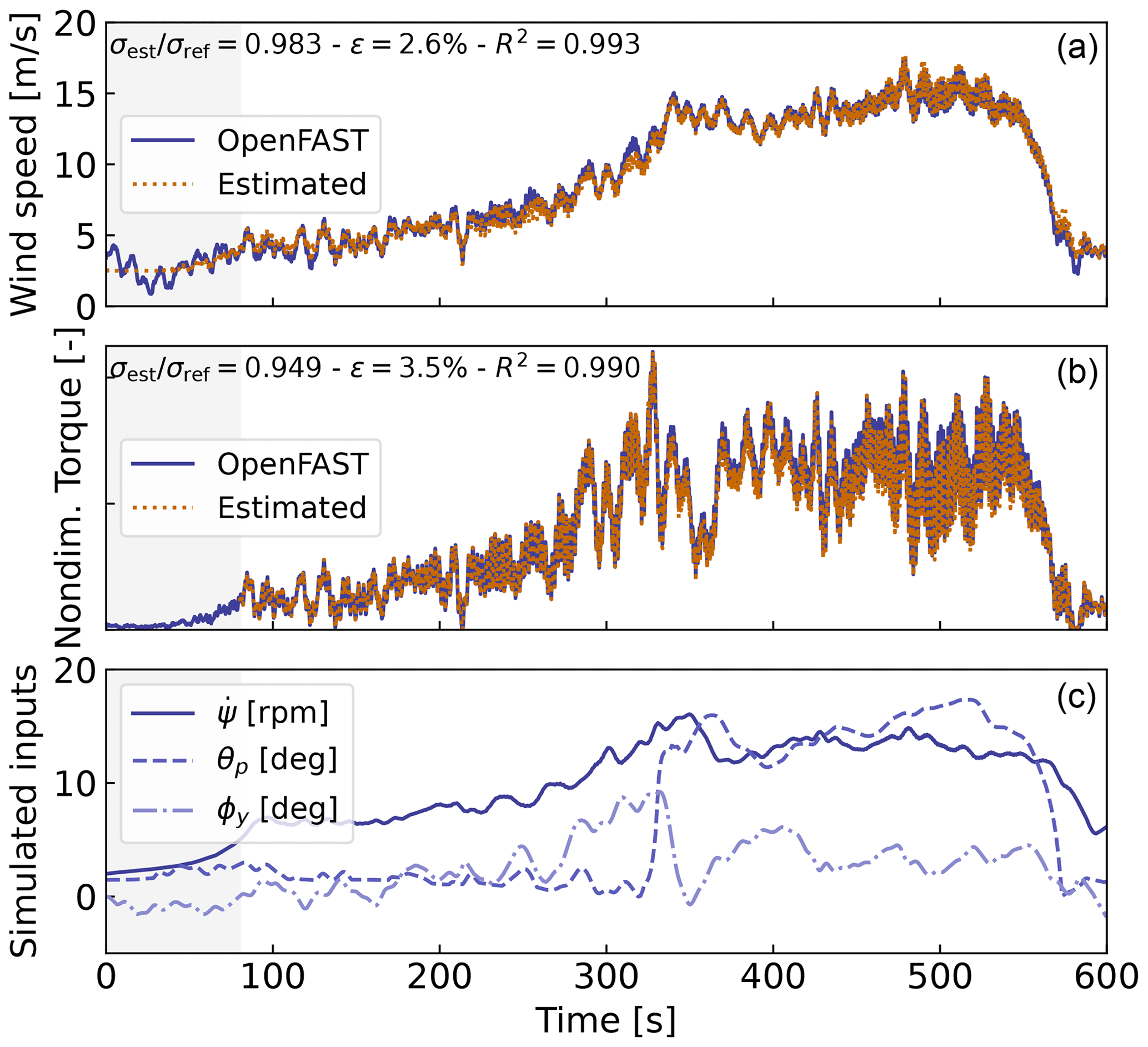
Figure 6Example of aerodynamic estimation using simulated measurements from OpenFAST. (a) Wind speed. (b) Dimensionless torque. c) Structural inputs from the OpenFAST simulation provided to the estimator.
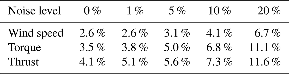
To quantify the performance of the estimator, we reproduce the simulation above but add different noise levels to the measurements to account for measurement errors by the sensors. A Gaussian noise signal of zero mean and standard deviation rσ is added to each input, where r is the noise level and σ is the standard deviation of the clean input. The results are shown in Table 4. As expected, the error in the estimation increases with increasing noise levels. This numerical experiment provides a rough quantification of the errors that can be expected from the aerodynamic estimator.
Table 4Mean relative error (ϵ) of the wind speed, torque, and thrust estimates for increasing noise levels.
3.5 State estimator
In this work, we follow a similar approach to our previous work (Branlard et al., 2020a), where an augmented Kalman filter is used to estimate states and loads. The Kalman filter used in the aerodynamic estimator (Sect. 3.4) is augmented with additional states and outputs. The Kalman filter uses two linear models: a state equation, describing the time evolution of the states, and an output equation, describing how the measurements are related to the states and inputs. The state and output equations are written as
where δxKF, δuKF, and δyKF are the state, input, and output,1 respectively; Xx, Xu, Yx, and Yu are the system matrices that relate the different system vectors; and wx and wy are Gaussian processes representing modeling noise. The output vector, δyKF, is also referred to as the “measurement” vector because it corresponds to the measured signals. At a given time step, the Kalman filter algorithm uses the system matrices, a set of measurements, and an a priori knowledge of the model and measurement uncertainties to estimate the state vector (Kalman, 1960; Zarchan and Musoff, 2015).
In this work, we design the state estimator such that the state vector contains the structural degrees of freedom (δq and ) and the aerodynamic torque (Q), and the input vector consists of the thrust (obtained with the aerodynamic estimator) and the generator torque (obtained from the power). These design choices were guided by our previous work on the topic. For this choice of state and input variables, we build linear models for the state and output equations. We use the linear models described in Sect. 3.3 (the A, B, C, and D matrices) to populate the system matrices of the Kalman filter. Additional details on how the relevant Jacobians are extracted are given in Sect. 3.6.1. Given our choice of system vectors, the state equation is
where A12 and A22 are the two lower blocks of the A matrix, and I is the identity matrix. The Jacobians with respect to the loads are extracted from the B and D matrices. A random walk approach is used for the evolution of the torque Q (that is, we set ). The output equation, which effectively relates the measurements to the system states and inputs, is set as
where is the vector of nacelle accelerations, and is the measurements of surge, sway, roll, and pitch as given in Table 1.
The state and output equations are used as part of a Kalman filter algorithm implemented in WELIB, which continuously takes as input the measurements from the wind turbine (corresponding to the left-hand side of Eq. 15). The process and covariance matrices used within the Kalman filter algorithm (determining the values of wx and wy) are populated based on the estimated standard deviations of the different states and outputs. At each time step, the thrust is estimated using the aerodynamic torque of the previous time step and used as input. The result of the Kalman filter is the estimated states and outputs at each time step. Sample simulation results are provided in Sect. 4.
3.6 Virtual sensing
Once the states are estimated by the Kalman filter, the virtual sensing step is used to derive quantities of interest (see Fig. 1). In this work, we focus on the estimation of the sectional loads along the tower using a physics-based model. We investigate two methods to obtain these loads.
3.6.1 OpenFAST linearization outputs
The first method consists of using the linearization outputs of OpenFAST, namely, using a subset of the equation (see Sect. 3.3.1). In general, if a quantity of interest is present in the output vector of OpenFAST, it can be retrieved as follows. If the variable is located at the row index k in the vector y, then this variable can be obtained from the states and inputs as
where [⋅]k indicates that the row k of the matrix or column vector is used. In our case, [y]k in Eq. (16) would be the sectional fore–aft bending moment at the height zj along the tower, noted ℳy(zj). The advantages of using this method are multiple:
-
the method is directly applicable to any other outputs computed by OpenFAST,
-
the calculation procedure is linear and therefore computationally efficient,
-
if strain measurements are available at given heights, the rows [C]k an[D]k could be included in the output equation of the Kalman filter (Eq. 15) to provide information about the model's expectation of these measurements, and
-
the underlying linear model is consistent with the nonlinear model of OpenFAST.
The downside of the method is its linearity, in the sense that it is only valid close to the operating point and could lack important nonlinear effects. The values of [C]k, [D]k, and [y0]k would potentially need to be reevaluated if the system operates away from the linearized operating point. One possible solution is to introduce gain scheduling to continuously modify the linear system based on the estimated wind speed. In this work, we used one operating point only and obtained results with fair accuracy (see Sect. 4). We nevertheless expect that to better represent the different operating regions of a pitch-regulated wind turbine, three to five linear models stitched together through gain scheduling would be needed.
3.6.2 Nonlinear calculation (WELIB)
An alternative method consists of computing the section loads based on first principles using the formulation presented in Branlard (2019). The calculation requires knowledge of the tower-top loads and the full kinematics of the tower and nacelle (position, velocity, and acceleration). At a given time step, the kinematics are computed based on q, , and . The tower-top loads are estimated based on the aerodynamic loads and the inertial loads of the rotor–nacelle assembly. We describe the method in more detail in Sect. D. The advantages are that nonlinearities are accounted for and the model is valid irrespective of the operating condition. The downside is that this method does not provide any of the four advantages offered by the OpenFAST linearization method.
3.6.3 Verification of the section load calculation
To verify the calculation of the section loads, we use the same turbulent step wind field and irregular sea state that were used in Sect. 3.4.4. We assume that the time series of q, and are entirely known, extracted from the OpenFAST simulation. These time series are provided to the two section loads algorithms: the WELIB nonlinear algorithm and the OpenFAST linear algorithm.
We run two sets of virtual sensing. In the “ideal” set, the loads at the tower top are extracted from OpenFAST results and provided to the two virtual sensing algorithms. In this ideal case, the linearized operating points of the OpenFAST linear model are set as the mean of each of the OpenFAST time series values. Results for the ideal case are illustrated in Fig. 7. The two algorithms are able to reproduce the section loads of OpenFAST with relatively high accuracy, which verifies our two calculation procedures.
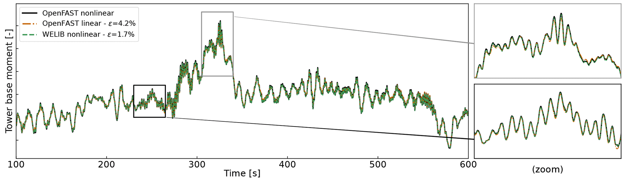
Figure 7Tower fore–aft bending moment for the turbulent step and an irregular sea state as calculated by OpenFAST and compared to the WELIB nonlinear and OpenFAST linear method. The motion of the structure is determined by OpenFAST and provided to the two algorithms. The tower-top loads are also provided to the algorithms (ideal case, as opposed to Fig. 8).
In the second set, labeled “unknown thrust”, the tower-top loads are not provided to the algorithms; instead, the aerodynamic estimator mentioned in Sect. 3.4.4 is used to estimate the aerodynamic loads. This time, we do not set the linearized operating point of the OpenFAST linear model to the mean value of the time series; we set it to the static equilibrium (without loading).
The results are illustrated in Fig. 8. The accuracy of the section load calculation is seen to deteriorate when the aerodynamic loads are estimated with the aerodynamic estimator, which is expected. The damage equivalent load computed with a Wöhler slope of m=5 is found to be 3.7 % lower with the OpenFAST linear method and 1.2 % lower with the YAMS nonlinear method compared to the value for reference signal.
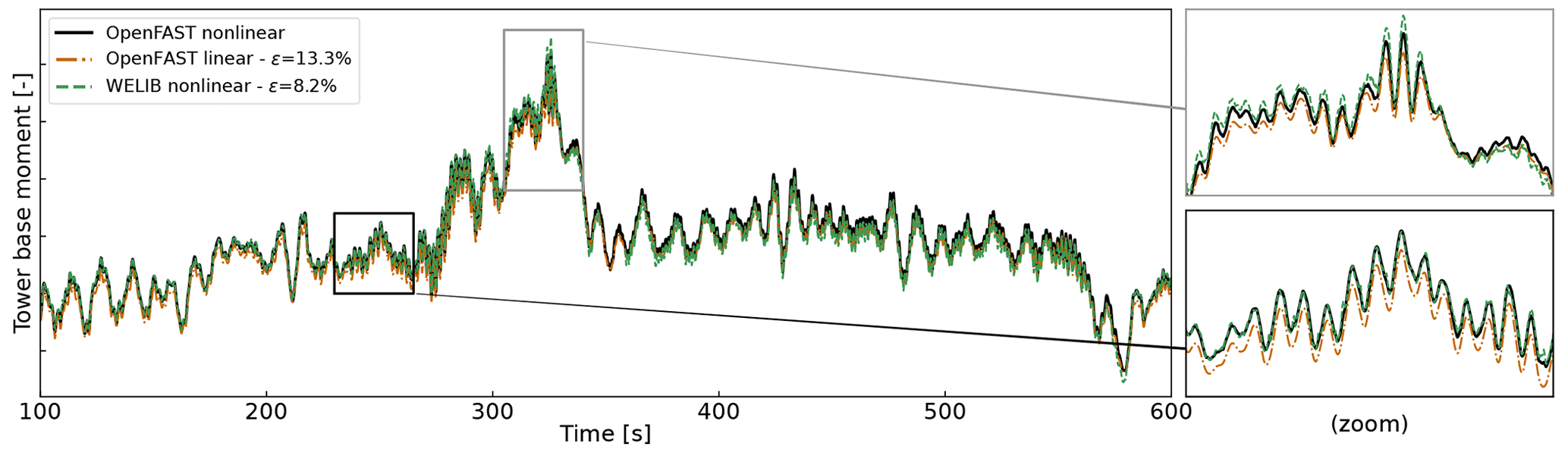
Figure 8Tower fore–aft bending moment for the turbulent step and an irregular sea state as calculated by OpenFAST and compared to the WELIB nonlinear and the OpenFAST linear method. The motion of the structure is determined by OpenFAST and provided to the two other algorithms. The tower-top loads are estimated using the aerodynamic estimator (unknown thrust case, as opposed to the ideal case presented in Fig. 7).
The performance of both algorithms remains satisfactory because the extrapolated signals follow the reference OpenFAST nonlinear simulation. The relative error obtained with the OpenFAST linear algorithm is higher (13.3 %) than the one obtained using the WELIB nonlinear method (8.2 %). The main source of error in the linear model is associated with the fact that the linearization point was not tuned for this specific simulation. It is our simplifying design choice to use only one linearization operating point throughout. Because of the loss of accuracy associated with this design choice, we use the WELIB nonlinear algorithm in the digital twin for the calculation of section loads.
After performing a sensitivity analysis on the inputs and states of the system, we observed that the variables that most affect the fore–aft section loads are the platform pitch (ϕy), the tower fore–aft bending degree of freedom (qt), and the aerodynamic thrust. In this section, we assumed that all the states were known (including ϕy and qt), leading to great accuracy in the estimation of the section loads. The final verification step involves providing estimated states to the algorithm, which is the topic of the next section.
In Sect. 3 we discussed how the different components of the digital twin were introduced and tested using increasing complexity. In this section, we discuss combining the different components to form the digital twin. We begin using numerical experiments from OpenFAST (see Sect. 2.3.2), similar to what was done previously, before using measurements from the TetraSpar prototype.
4.1 Numerical experiment
First, we use the same turbulent step wind field and sea state that was used throughout Sect. 3. The augmented states of the system are determined at each time step using the state estimator described in Sect. 3.5. The measurements (see Table 1) are taken from the nonlinear OpenFAST simulation. The wind speed and aerodynamic loads are estimated using the aerodynamic estimator described in Sect. 3.4. The linear model is derived from linearized OpenFAST, and the section loads in the tower are obtained using the WELIB virtual sensing algorithm described in Sect. 3.6. The estimates from the digital twin are compared with the reference nonlinear OpenFAST simulation results in Fig. 9. A visual inspection of the time series reveals that the digital twin is able to capture the main trends and fluctuations of the different signals. The match can be considered remarkable given that only the sensors provided in Table 1 are used by the digital twin. Metrics such as mean relative error (ϵ) and coefficient of determination (R2) are indicated on the figure. Despite the visually appealing match, the metrics indicate that the tower-bottom moment has a mean error of ϵ=21 %. The damage equivalent load of the tower-bottom moment is underestimated by %, where we define
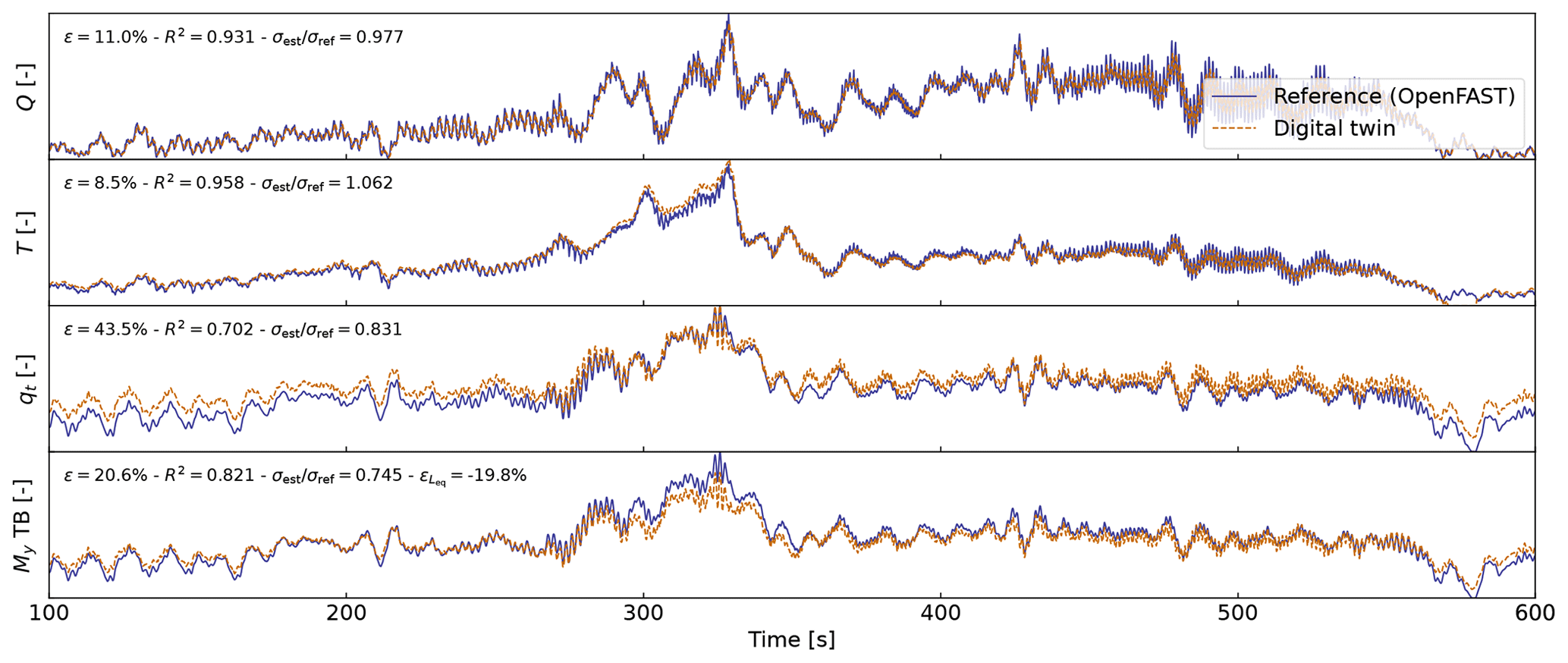
Figure 9Estimated signals from the digital twin compared to results from a nonlinear OpenFAST simulation using the turbulent-step numerical experiment. From top to bottom: aerodynamic torque (Q), aerodynamic thrust (T), tower-top position (qt), and tower-bottom fore–aft bending moment (My, TB). Results are made dimensionless for confidentiality reasons.
Differences in damage equivalent loads typically indicate differences in the frequency content of the signals. We compare the frequency content of the estimated signals with the reference signals in Fig. 10. The low-frequency content (below 1 Hz) is captured well, in line with the visual inspection of Fig. 9. Unfortunately, no clear trend is found for the high-frequency content: the power spectra of the aerodynamic loads indicate an underestimation, whereas the spectra of the tower-top position and tower-bottom bending moment tend to have higher energy content. As shown in previous studies (Branlard et al., 2020a), filtering of the input measurements can be used to tune the energy content at high frequencies. The method is yet unsatisfactory because it acts as an artificial rebalancing of energy content to achieve the desired DEL value. Both low- and high-frequency content contribute to the DEL values; therefore, we believe that systematic improvement is only possible through modeling improvements and higher observability of the states by the Kalman filter.
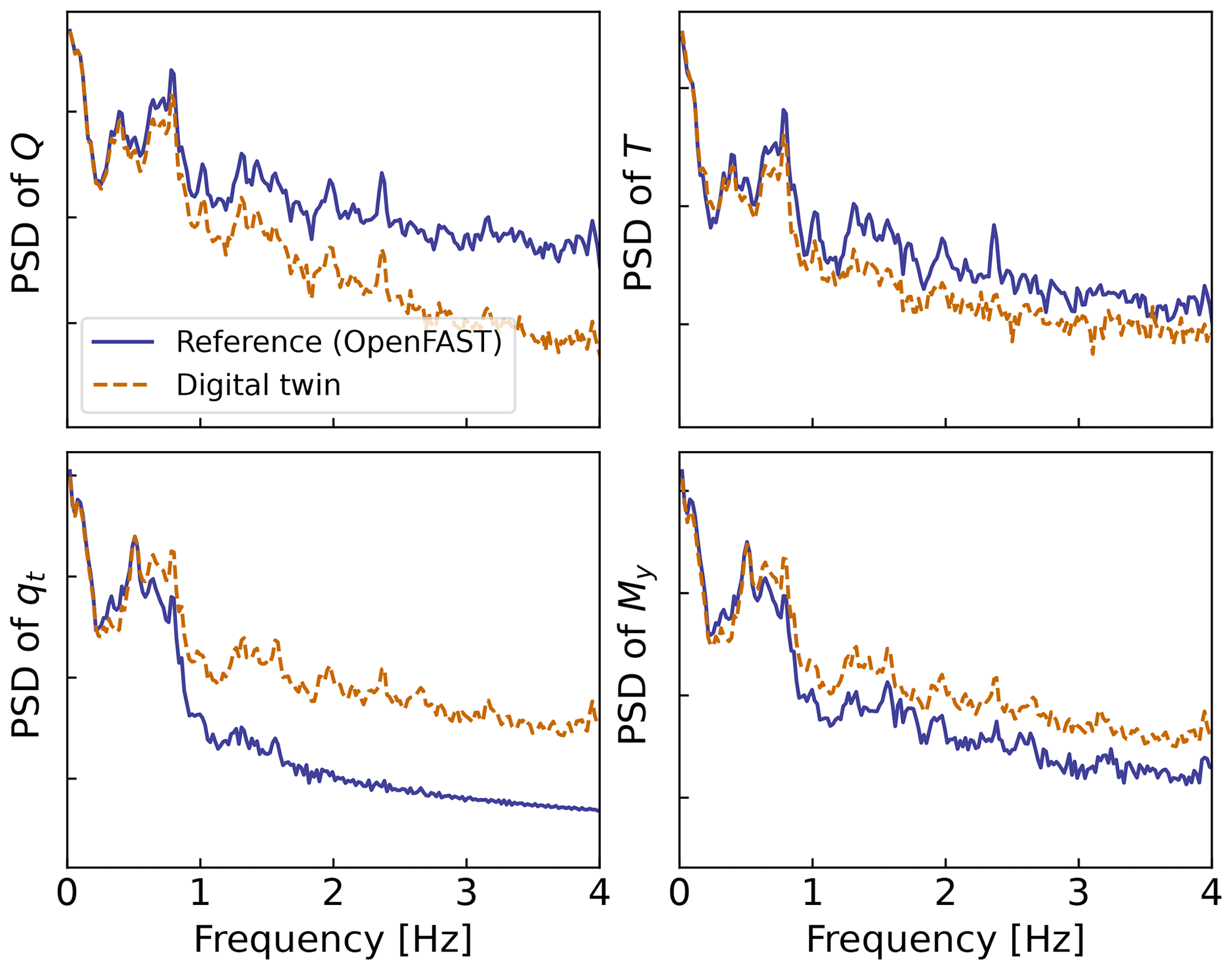
Figure 10Power spectral density (PSD) of the time series presented in Fig. 9. A logarithmic scale is used on the y axis.
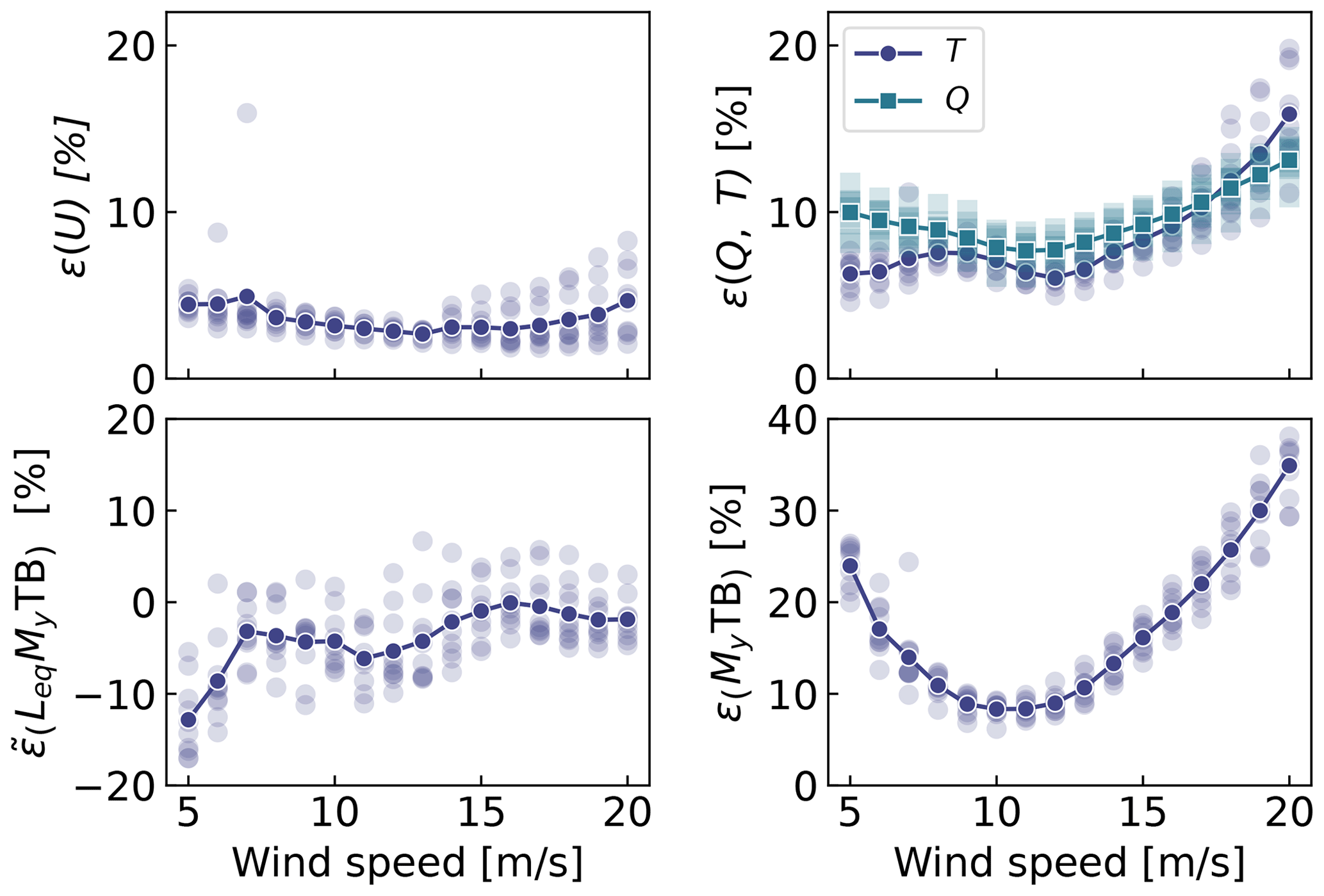
Figure 11Mean relative error of estimated signals for various wind speed and seeds. Clockwise from top left: wind speed (U), aerodynamic loads, tower-bottom moment (My TB), and damage equivalent load of the tower-bottom moment ( TB). The individual simulations are indicated by transparent markers. The average over each seed is indicated using solid lines.
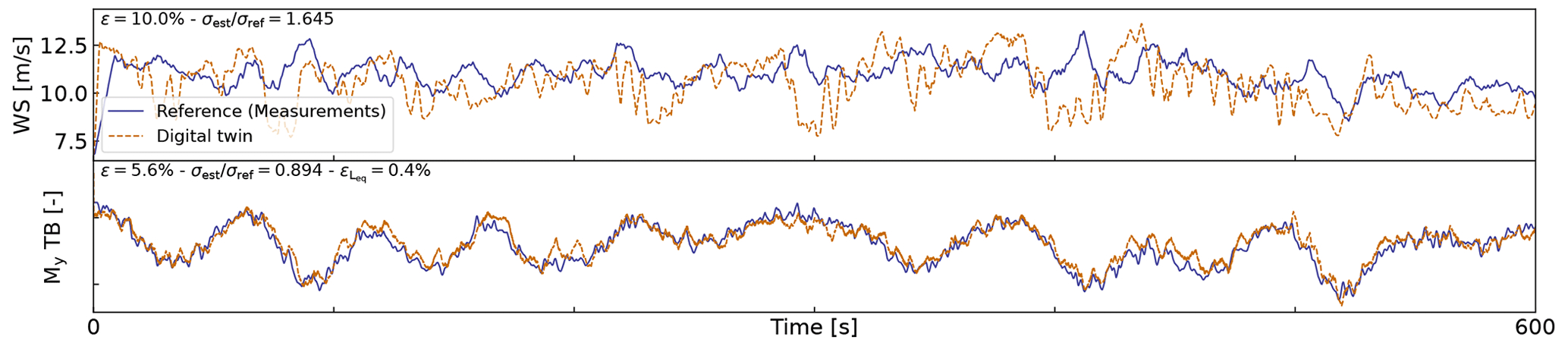
Figure 12Comparison of digital twin outputs with wind speed and tower-bottom moment measurements from the TetraSpar prototype. The measured wind speed comes from a nacelle anemometer and therefore is expected to differ from the rotor-averaged value estimated by the digital twin.
To quantify the errors in the estimation under a wider set of operating conditions, we run 10 min simulations for a set of wind speeds under normal turbulent conditions and sea states. We select wind speeds from 5 to 20 m s−1 using 10 different seeds per bin of wind speed. The seeds are used to randomize the turbulent field and sea states. The wind speed range is selected so as to avoid cut-in and cut-out events where the aerodynamic estimator is not expected to perform well. The turbulence intensity is selected based on the normal turbulence model for a turbine of class A. The wave height and wave period are set as a function of the wind speed as and . The Hs and Tp relationships were obtained by performing a linear regression on the sea state and wind measurements at the test site. OpenFAST simulations are run for each case, and then the digital twin is run using these numerical measurements. A summary of the mean relative error on some key estimated quantities is given in Fig. 11. We observe that the mean relative error of the wind speed and aerodynamic loads is between 5 % and 15 % with a tendency for larger errors on the aerodynamic loads at low and high wind speeds. The error further propagates within the system, and the tower-bottom moment is estimated with a relative error between 10 % and 40 %. The error levels indicate that the aerodynamic estimator, which is based on quasi-steady rotor-averaged aerodynamics, cannot fully capture the dynamic aerodynamic state of the rotor in floating conditions. In general, the digital twin lacks sufficient information to fully capture the tower-top loads and the frequency content of the system. It is expected that the placement of additional sensors, such as accelerometers or load cells, along the tower can significantly improve the estimation of the tower loads (in that case, we would either use OpenFAST linearization outputs or an extended Kalman filter and a nonlinear model for the outputs). As seen in Fig. 11, the relative error levels on the damage equivalent loads are between −10 % and 5 %, with the loads being either overestimated or underestimated depending on the wind speed. The structural health monitoring system could potentially use the estimated error levels indicated in Fig. 11 to provide a confidence interval on the fatigue lifetime of the tower. We note that these error levels represent a best-case scenario because we assumed that no noise or biases were present in the measurements. We expect the error levels to increase with additional measurement noise.
4.2 Estimations using measurements from the full-scale prototype
In this section, we use measurements from the full-scale TetraSpar prototype installed off the Norwegian coast. Four days of data were selected based on data availability; a wide range of wind speeds are present in the time series (ranging from 4 to 24.5 m s−1 with an overall mean of 8.9 m s−1). Two days were selected in summer and two in winter to account for potential seasonality. Apart from these criteria, the selection of time series can be considered random. The measurement data are stored as 10 min time series sampled at 25 Hz. The total number of 10 min samples used over the four days is 576. The measurement data are provided to the digital twin to perform the state estimation and virtual sensing. The prototype is equipped with load cells at the tower top, middle, and bottom and nacelle wind speed measurements. We use these measurements to compare with the digital twin estimates.
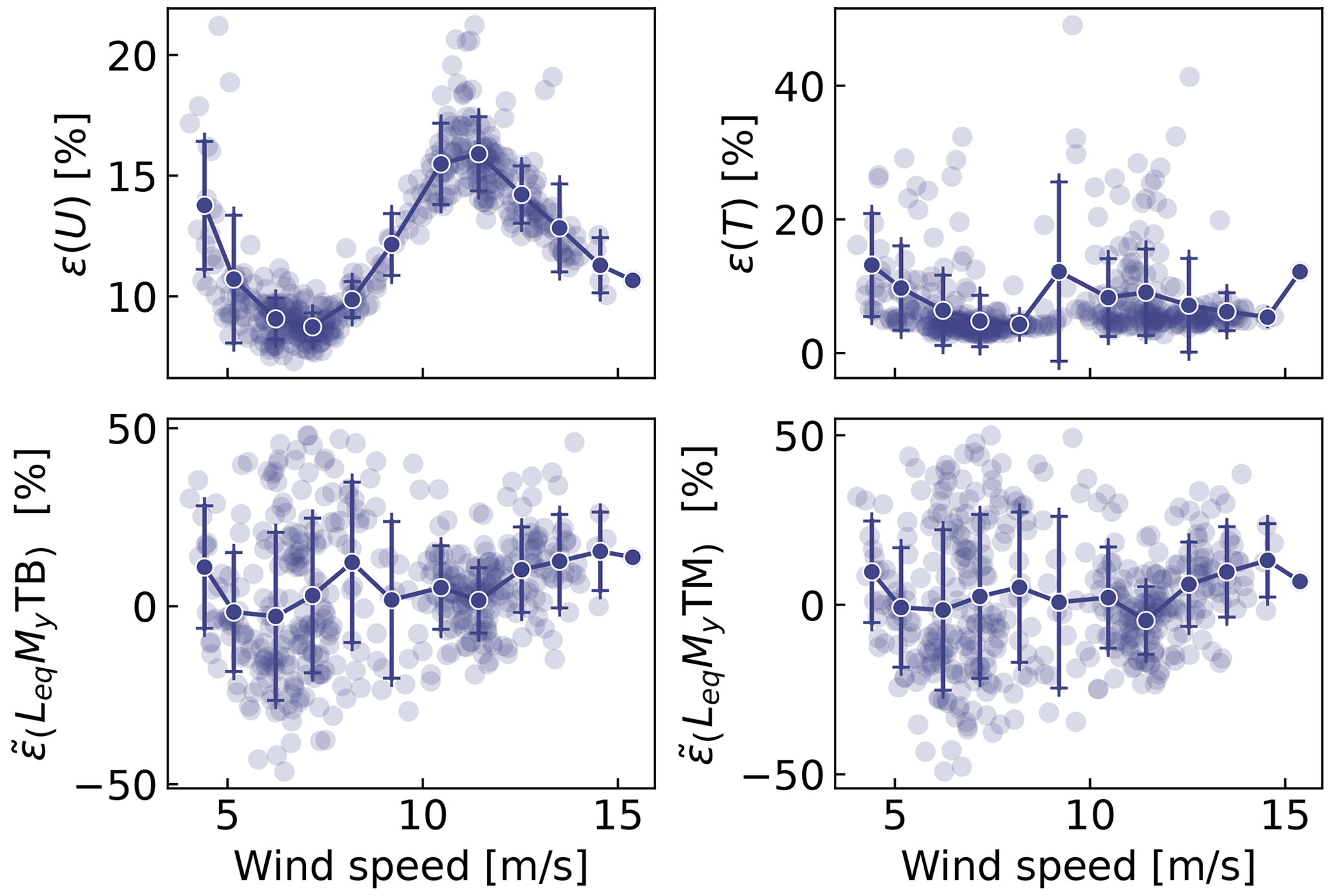
Figure 13Similar to Fig. 11 but using measurements from the TetraSpar prototype. Each marker indicates a 10 min simulation result. Solid lines are bin averages. The whiskers indicate the standard deviation in each bin. The bottom plots are for the tower-bottom (TB) and tower-middle (TM) bending moments.
We begin by highlighting the computational time of the current procedure, as computational efficiency is crucial to achieve our digital twin vision. The state estimation is currently 10 times faster than real time. The virtual sensing step is twice as fast as real time, but computational improvements are possible, in particular, by using a compiled language instead of Python. For reference, OpenFAST simulations of the full TetraSpar model (with substructure flexibility) typically run 3 times slower than real time, and a reduced-order OpenFAST model with 8 DOFs runs 1.1 times slower. Currently, real time estimation cannot be achieved with OpenFAST. Reduced-order modeling techniques, such as the ones presented in this article, are necessary to implement an online digital twin. Yet, if the digital twin is run as a postprocessing step, then parallelization using multiple CPUs could be used, e.g., processing different time periods of the day.
A sample of results is provided in Fig. 12. The figure illustrates a selected case where the estimation of the tower load is reasonably accurate, with an error on the damage equivalent load of only 0.4 %. We note that the wind speed from the measurement is a point measurement (from the nacelle anemometer, in the wake of the turbine, and moving with the nacelle), and it is therefore not expected to be in strong agreement with the digital twin estimate, which is representative of a rotor-averaged wind speed.
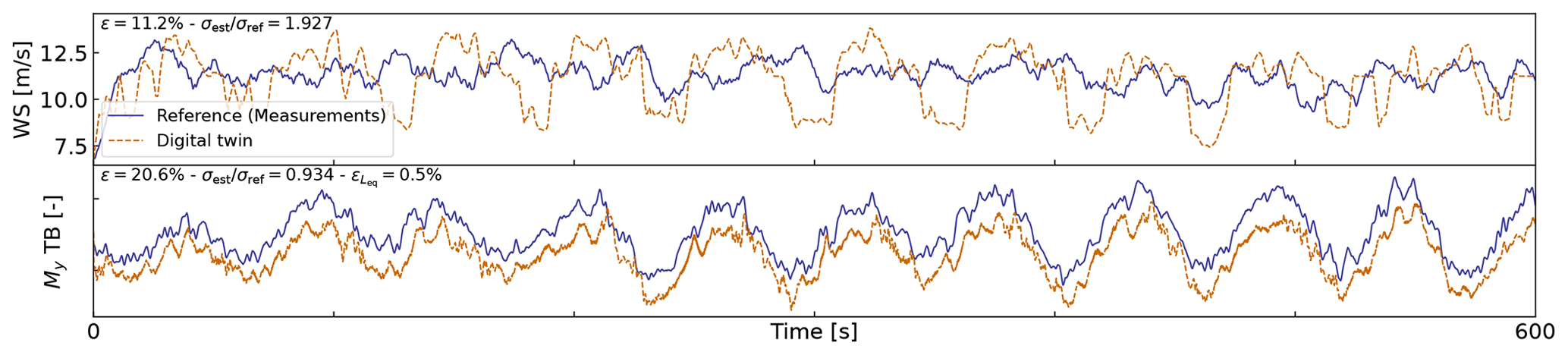
Figure 14Similar to Fig. 12 but for a case where a clear offset is present in the tower loads.
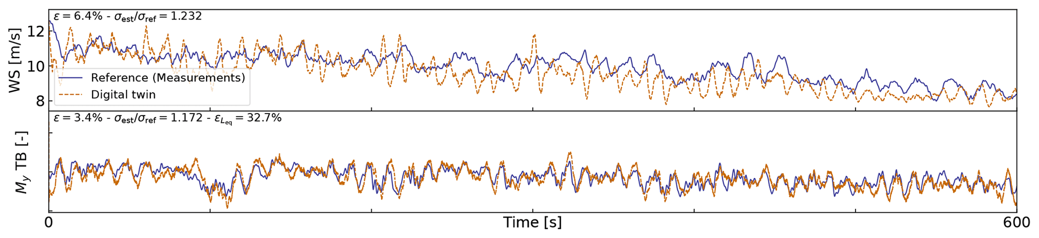
Figure 15Similar to Fig. 12 but for a case where a large error in damage equivalent load is observed.
An aggregate of results from all the 10 min digital twin runs is illustrated in Fig. 13. The figure shows relative errors in wind speed, thrust, and damage equivalent loads at the tower bottom and tower middle. As indicated previously, the wind speed from the digital twin and the measurements are different quantities, but the level of error obtained indicates that the digital twin is able to capture the main level of wind speed. The aerodynamic thrust from the aerodynamic estimator is compared with the load cell at the tower top in the fore–aft direction. This is a crude first-order approximation (e.g., neglecting inertial and gravitational loads, nacelle tilting, and shaft bending), but the overall estimated levels appear to be, on average, around 10 % of those obtained from the measured ones. The tower damage equivalent loads are, on average, within ±10 % of the values obtained from the measurements, but some cases show errors ranging between ±50 %. To give perspective on the large error values taken by the metrics, we illustrate two cases with large errors in Figs. 14 and 15. In both cases, we observe that the estimator is capturing the trends and low frequencies with accuracy that, from a pure qualitative perspective, would appear satisfactory. As seen in Fig. 14, an offset is present in the signal, which indicates that some physics might be missing from the load virtual sensing or that the state estimator is failing. Measurement errors could also affect the results, but no systematic error was detected over the time period investigated. It is therefore difficult to conclude as to what is the main source of error. In Fig. 14, the overall load level is captured well, but the error in the damage equivalent load is is 33 %. As illustrated in Fig. 10, our current method fails at capturing the high-frequency content of the signals, which can have a significant impact on the accuracy of the damage equivalent loads. Despite these challenges, the average accuracy of 10 % is promising and indicates that the current methodology can be used to reconstruct some structural and environmental signals from a limited number of readily available sensors.
In this work, we implemented, verified, and validated a physics-based digital twin solution applied to a floating offshore wind turbine. The work focused on the estimation of the aerodynamic loads and the section loads along the tower, using a set of measurements that we expect to be available on any existing wind turbine (power, pitch, rotor speed, and tower acceleration) and motion sensors that are likely to be standard measurements for a floating platform (inclination and GPS sensors). The key concept behind our approach uses
-
a Kalman filter to estimate the structural states based on a linear model of the structure and measurements from the turbine,
-
an aerodynamic estimator, and
-
a physics-based virtual sensing procedure to obtain the loads along the tower.
An important part of the work was developing the methodology and implementing the tools and models necessary for the aerodynamic estimation, state estimation, and load virtual sensing. We explored two different pathways to obtain models: a suite of Python tools and OpenFAST linearization. We used components from both approaches for the digital twin.
Using numerical experiments, we found that the accuracy of the individual models was typically on the order of 5 %. When comparing the digital twin estimations with the measurements from the TetraSpar prototype, the errors increased to 10 %–15 % on average for the quantities of interest. Overall, the accuracy of the results appeared promising given the scope of our work, which aimed to illustrate a proof of concept for a floating wind turbine digital twin. We observed a non-negligible scatter of results for the estimation of the tower damage equivalent loads that we attributed to the difficulty of capturing high-frequency content.
Future work should therefore explore possible improvements of the method to address this issue.
Additional improvements could include
-
gain scheduling of the linear models to extend the domain of validity of the linear models used and reduce the modeling error;
-
using nonlinear models and extended Kalman filtering techniques to lift the linear assumptions that challenge the aerodynamics, hydrodynamics, and structural dynamics;
-
introducing additional degrees of freedom and a full account of the yawing of the nacelle to increase the fidelity of the models and account for the flexibility of the floater;
-
adding a model to account for wave-excitation forces to account for hydrodynamic loads and likely improve the estimation of member-level loads;
-
introducing additional measurements to improve the state estimation and increase the observability of the state;
-
improving the robustness of the aerodynamic estimator in particular, beyond the cut-in and cut-out wind speeds, to apply the digital twin when the turbine is not operating; and
-
expanding the virtual sensing steps to estimate additional signals.
In this section, we describe the procedure used to linearize the structural equations of motion without knowledge of the external loads, which is used to obtain Eq. (1). We write the implicit form of the equations of motion as
where q, , , and are the degrees of freedom, velocities, accelerations, and augmented inputs of the model, respectively. The term augmented input is used because the external loads are included in this vector. The external loads are (in general) a function of the degrees of freedom. Therefore, we write the augmented input vector as
where u is the vector of inputs in the classical sense, that is, consisting of system inputs that do not depend on the degrees of freedom (for instance, the wave elevation). The operating point is written using the subscript “0” and is defined as
We perturb each variable, as , , etc., where δ indicates a small perturbation of the quantities. The perturbation of the augmented input is then
where |0 indicates that the expressions are evaluated at the operating point. The linearized equations are obtained using a Taylor-series expansion:
with
and where M0, C0, and K0 are the linear mass, damping, and stiffness matrices, and Q0 is the linear forcing vector, also called the input matrix.
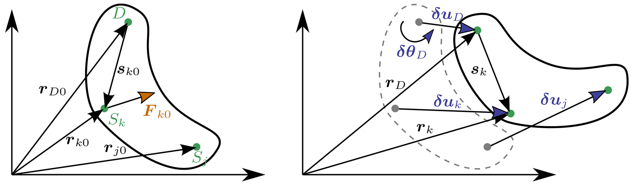
The Jacobians provided by OpenFAST and MAP are provided at given nodes of the structure (e.g., the hydrodynamic nodes, or the fairleads). In this section, we highlight the procedure to transfer these Jacobians to another node (the platform reference point) assuming a rigid-body relationship between the nodes. The procedure is used in this work to compute the linear 6×6 matrix for the hydrodynamics and mooring dynamics in Sect. 3.3.2. We obtain different relationships depending on whether the destination point is assumed to be displaced or not (see different subsections below).
B1 Transfer of Jacobians between two points
We consider a point source (noted S) and a destination point (noted D). The notations are illustrated in Fig. B1. We assume that the two points belong to a rigid body. The forces and moments at the destination and source are related as follows:
where is the vector from destination point to the source point; FS and MS are the force and moments, respectively, at point S; and the tilde notation refers to the skew symmetric matrix, which is a matrix representation of the cross product. We seek to linearize Eqs. (B1) and (B2) for small displacements and rotations of the destination and source nodes. In particular, we seek to express the Jacobians at the destination node as a function of the source node, assuming a rigid-body relationship between the two. The rigid-body relationship linking the small displacements (δu) and small rotations (δθ) of the source and destination points is
where s0 is the vector between the source and destination points at the operating point (prior to the perturbation). The Jacobians of the transformations given in Eq. (B3) and its inverse are
To linearize Eqs. (B1) and (B2), we introduce the following perturbations:
where the subscript 0 indicates values at the operating point. At the operating point, Eqs. (B1) and (B2) are satisfied; that is,
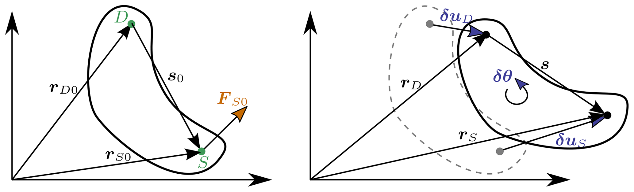
Figure B1Rigid-body kinematics with the loads from one source point (S) transferred to a destination point (D), assuming small motion of the points.
B1.1 Transfer of forces
Inserting Eq. (B5) into Eq. (B1) leads to
which, using Eq. (B7), leads to
The Jacobians of the loads at node D with respect to the displacements at node D are then obtained by applying the chain rule to Eq. (B10) and making use of the Jacobian of the displacements given on the right of Eq. (B4). For instance, for the force,
For the transfer of the moments, the relationship will be different whether the moments are transferred at the undisplaced destination point or the displaced destination point.
B1.2 Moments at the undisplaced destination point
In this section, the moments are transferred to the undisplaced destination point. The vector from the undisplaced destination point to the displaced source is
Introducing Eqs. (B6) and (B12) into Eq. (B2) and temporarily using the “×” notation instead of the tilde notation leads to
Making use of Eq. (B8), neglecting the nonlinear term (δuS×δFS), and reintroducing the tilde notation leads to
The Jacobians of the moments at the undisplaced node D with respect to the displacements at node D are then obtained by applying the chain rule to Eq. (B14):
and
B1.3 Jacobian relationships at the undisplaced destination point
Equations (B11), (B16), and (B15) can be gathered in matrix form to relate the different Jacobians between the source point and the undisplaced destination point:
B1.4 Moments at the displaced destination point
In this section, the moments are transferred to the displaced destination point. The vector from the displaced destination point to the displaced source is
Introducing Eqs. (B6) and (B18) into Eq. (B2) and temporarily using the “×” notation instead of the tilde notation leads to
Making use of Eq. (B8), neglecting the nonlinear term (), and reintroducing the tilde notation leads to
The Jacobians of the loads at the displaced node D with respect to the displacements at node D are then obtained by applying the chain rule to Eq. (B20) and making use of the Jacobian of the displacements given on the right of Eq. (B4).
and
B2 Relationships at the displaced destination point for multiple source points
We now consider the case where multiple point sources are present. The derivation can be seen as a generalization of the previous case between two points, but special care is needed when summing the contributions from the different nodes. The notations are illustrated in Fig. B2. The loads at the destination points are obtained as
where k is an index looping over all points of the rigid structure. To shorten notations, we define the vector between the destination point and a given point as
where sk is the vector between the displaced points and is the vector prior to the displacement. Due to the rigid-body assumption, the elementary displacements of the points are related as follows:
from which one obtains the relationships
Using a similar Taylor expansion as for the case with two nodes, the perturbation loads are obtained as
The chain rule for a given quantity of interest (Q) is obtained by summing over all the elementary variables:
For instance, applying the chain rule to FD and using Eq. (B30) leads to
Eventually, the Jacobians at the displaced destination node are obtained as
In this section, we supplement the results given in Sect. 3.3.3 by showing free-decay results without hydrodynamics (no added mass, damping, hydrostatics). In Fig. C1, we show results with the structure only, and results with the structure and moorings are reported in Fig. C2. These results also include the nonlinear WELIB formulation. A strong agreement is found between the nonlinear OpenFAST and WELIB models and between the linear OpenFAST and WELIB models. The yaw degree of freedom appears to be more challenging to capture for the linear models. We recall that OpenFAST and WELIB use a different definition of the transformation matrices between the degrees of freedom, which results in different structural dynamic equations.
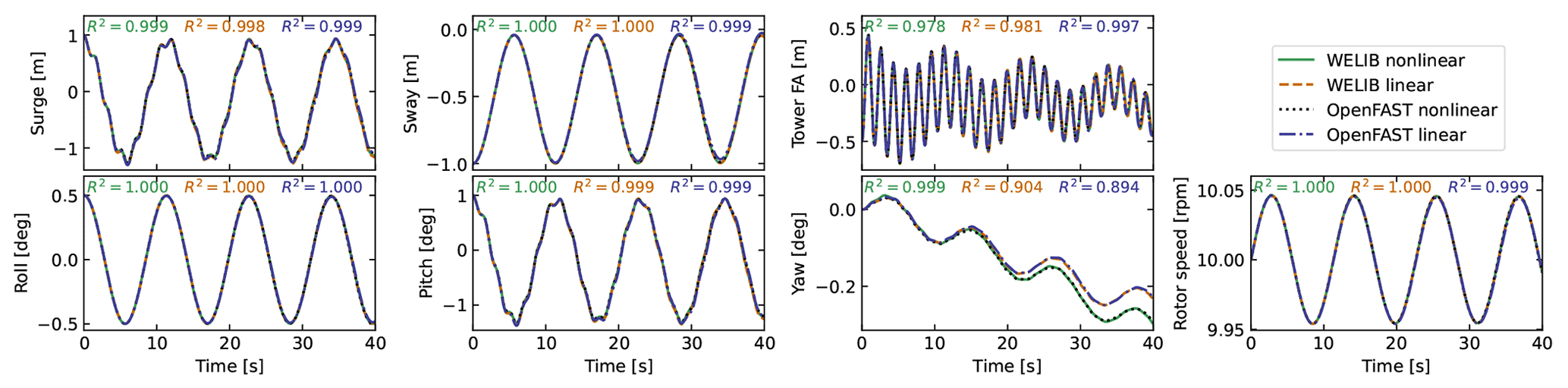
Figure C1Free decay of the structure using nonlinear and linear models for a case including only the structure (no moorings, no hydrodynamics). Time series of the main DOFs.
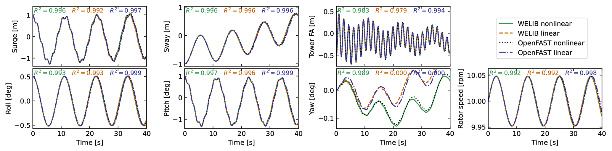
Figure C2Free decay of the structure using nonlinear and linear models for a case including moorings (no hydrodynamics). Time series of the main DOFs.
In this section, we describe the nonlinear calculation procedure used in Sect. 3.6.2 to assess the section loads along the tower based on estimates of the structure kinematics and the loads at the tower top. For conciseness, in this appendix, we use x and z for the coordinates along the tower fore–aft and tower height, respectively, instead of xT and zT.
D1 Tower fore–aft bending moment and shear force
The fore–aft and side–side moments are computed in the same way; therefore, this section focuses on the fore–aft direction. The sectional fore–aft bending moment at a given tower height z is determined as
Here, ℳy,top is the fore–aft bending moment at the tower top, and Sx is the shear force in the x direction, obtained as
where px,all is the force per unit length acting on the tower section in the fore–aft direction, including contributions from the external loads (aerodynamic loads on the structure), inertial loads due to the acceleration of the structure (including gravity), and nonlinear correction terms from the loads in the z direction (p−Δ effect, including self-weight effects). The different contributions are written as follows:
In this work, we neglect the external loads on the tower, (aerodynamic loads on the tower are typically small relative to rotor-thrust loads for an operating wind turbine). The acceleration contribution is , where m is the mass per length along the beam, ax,struct(z) is the acceleration of the section, determined based on the rigid-body acceleration of the floater and the elastic motion of the tower ( and ), and ax,grav is the acceleration of gravity in the x direction. The p−Δ correction term due to the vertical loading is computed as (see Branlard, 2019)
where pz is the vertical load per unit length (mostly consisting of the self-weight), ℱz,k is the kth vertical force acting at point zk, δ is the Dirac function, and Φ is the shape function used to describe the tower displacement field (see Sect. 2.3.3). In our case, only the vertical force acting on top of the tower is present, z1=LT, and . The procedure to compute the section loads in the y direction (using the p−Δ correction as well) is similar.
D2 Tower and rotor–nacelle assembly kinematics
The determination of the tower section loads requires knowledge of the tower kinematics, to compute astruct, and of the rotor–nacelle assembly (RNA) kinematics, to compute the inertial contribution to the tower-top loads (see Sect. D3). The position, linear velocity, linear acceleration, rotational speed, and rotational acceleration of the floater (point F, body f) are given respectively by
where the notation i indicates that the coordinates of the vector are expressed in the inertial coordinate system. The transformation matrix from the floater to the inertial frame is obtained as , where R is a function computing the rotation matrix. The tower base (point T, body t) kinematics are obtained from the floater motion using rigid-body kinematics:
where rFT is the vector from the floater point to the tower base. The kinematics of a given tower section (point S, at height z) are given by
where is the vector from the tower base to the undeflected section, and uS, , and are the elastic motions of the section computed based on the shape function and the generalized coordinates, e.g., (see Branlard and Geisler, 2022). We note that OpenFAST also includes a vertical motion associated with the deflection (referred to as a “geometric nonlinearity”), which we neglect in this work. The transformation matrix from the section to the tower is , where uS,y and uS,x are the components of uS in the tower coordinate system, and the prime notation indicates the differentiation with respect to z. The rotation speed and acceleration of the tower section with respect to the tower base are
The kinematics of the tower-top point and nacelle (point N, body n) are taken from the last section node (point S with z=LT). Yawing, tilting, and rolling of the tower top would change the orientation matrix, rotational velocity, and rotational acceleration of the nacelle. These kinematics are omitted here for conciseness. The kinematics of the center of mass of the RNA (point G) are obtained using rigid-body kinematics – identical to what was used between point F and T.
D3 Tower-top loads
The tower-top loads are computed as follows:
where the aerodynamic loads are transferred to the tower top and where the inertial loads from the rigid-body RNA are
where rNG is the vector from the tower top to the center of mass of the RNA, MRNA is the mass of the RNA, JG is the inertia tensor of the RNA at its center of mass, aG is the linear acceleration of the center of mass of the RNA, ωn is the rotational acceleration of the RNA, and is the rotational acceleration of the nacelle. The load calculation is first done in the coordinate system of the nacelle and then transferred to the coordinate system of the tower where Eq. (D1) is defined.
The source code of the digital twin and examples using a generic spar turbine are provided in the GitHub repository (https://github.com/NREL/wtDigiTwin, Branlard, 2023a) and https://doi.org/10.5281/zenodo.8048549 (Branlard, 2023b).
The wind turbine model and measurement data for the TetraSpar are not publicly available. The source code repository (see “Code availability”) contains open-source models of the NREL 5 MW for testing purposes.
EB implemented the digital twin and wrote the main corpus of this paper. JJ, CB, and JZ provided continuous feedback on the project and reviewed the article.
At least one of the (co-)authors is a member of the editorial board of Wind Energy Science. The peer-review process was guided by an independent editor, and the authors also have no other competing interests to declare.
Publisher's note: Copernicus Publications remains neutral with regard to jurisdictional claims made in the text, published maps, institutional affiliations, or any other geographical representation in this paper. While Copernicus Publications makes every effort to include appropriate place names, the final responsibility lies with the authors.
The views expressed in the article do not necessarily represent the views of the DOE or the US Government.
This research has been supported by the US Department of Energy Office of Energy Efficiency and Renewable Energy Wind Energy Technologies Office, under the Technology Commercialization Fund grant no. TCF-21-20 24800.
This paper was edited by Alessandro Croce and reviewed by Alessandro Fontanella and three anonymous referees.
Abbas, N. J., Zalkind, D. S., Pao, L., and Wright, A.: A reference open-source controller for fixed and floating offshore wind turbines, Wind Energ. Sci., 7, 53–73, https://doi.org/10.5194/wes-7-53-2022, 2022. a
Auger, F., Hilairet, M., Guerrero, J. M., Monmasson, E., Orlowska-Kowalska, T., and Katsura, S.: Industrial Applications of the Kalman Filter: A Review, IEEE Trans. Indust. Elect., 60, 5458–5471, https://doi.org/10.1109/TIE.2012.2236994, 2013. a
Bilbao, J., Lourens, E.-M., Schulze, A., and Ziegler, L.: Virtual sensing in an onshore wind turbine tower using a Gaussian process latent force model, Data-Cent. Eng., 3, e35, https://doi.org/10.1017/dce.2022.38, 2022. a
Bossanyi, E. A.: Individual Blade Pitch Control for Load Reduction, Wind Energy, 6, 119–128, https://doi.org/10.1002/we.76, 2003. a
Bottasso, C. and Croce, A.: Cascading Kalman Observers of Structural Flexible and Wind States for Wind Turbine Control, Tech. rep., Scientific Report DIA-SR 09-02, Dipartimento di Ingegneria Aerospaziale, Politecnico di Milano, Milano, Italy, https://www.researchgate.net/publication/228941698 (last access: January 2024), 2009. a
Boukhezzar, B. and Siguerdidjane, H.: Nonlinear Control of a Variable-Speed Wind Turbine Using a Two-Mass Model, IEEE Trans. Energ. Convers., 26, 149–162, https://doi.org/10.1109/TEC.2010.2090155, 2011. a
Branlard, E.: Flexible multibody dynamics using joint coordinates and the Rayleigh-Ritz approximation: The general framework behind and beyond Flex, Wind Energy, 22, 877–893, https://doi.org/10.1002/we.2327, 2019. a, b, c
Branlard, E.: wtDigiTwin GitHub repository, GitHub [code], https://github.com/NREL/wtDigiTwin (ast access: June 2023), 2023a. a
Branlard, E.: Digital twin modeling framework for wind turbines, Zenodo [code], https://doi.org/10.5281/zenodo.8048549, 2023b. a
Branlard, E.: WELIB, Wind Energy Library, GitHub [code], http://github.com/eBranlard/welib/ (last access: June 2023), 2023c. a
Branlard, E.: welib (1.0), Zenodo [code], https://doi.org/10.5281/zenodo.8048349, 2023d. a
Branlard, E. and Geisler, J.: A symbolic framework to obtain mid-fidelity models of flexible multibody systems with application to horizontal-axis wind turbines, Wind Energ. Sci., 7, 2351–2371, https://doi.org/10.5194/wes-7-2351-2022, 2022. a, b, c
Branlard, E., Giardina, D., and Brown, C. S. D.: Augmented Kalman filter with a reduced mechanical model to estimate tower loads on a land-based wind turbine: a step towards digital-twin simulations, Wind Energ. Sci., 5, 1155–1167, https://doi.org/10.5194/wes-5-1155-2020, 2020a. a, b, c, d
Branlard, E., Jonkman, J., Dana, S., and Doubrawa, P.: A digital twin based on OpenFAST linearizations for real-time load and fatigue estimation of land-based turbines, J. Phys.: Con. Ser., 1618, 022030, https://doi.org/10.1088/1742-6596/1618/2/022030, 2020b. a, b
Castella, X. T.: Operations and maintenance costs for offshore wind farm analysis and strategies to reduce O&M costs, MS thesis, Universitat Politècnica de Catalunya, and National Taiwan University of Science and Technology, https://upcommons.upc.edu/bitstream/handle/2117/329731/master-thesis-xavier-turc-castell-.pdf (last access: January 2024), 2020. a
Cosack, N.: Fatigue Load Monitoring with Standard Wind Turbine Signals, PhD thesis, Universität Stuttgart, https://d-nb.info/1009926721/34 (last access: January 2024), 2010. a
Dimitrov, N., Kelly, M. C., Vignaroli, A., and Berg, J.: From wind to loads: wind turbine site-specific load estimation with surrogate models trained on high-fidelity load databases, Wind Energ. Sci., 3, 767–790, https://doi.org/10.5194/wes-3-767-2018, 2018. a
Eftekhar Azam, S., Chatzi, E., and Papadimitriou, C.: A dual Kalman filter approach for state estimation via output-only acceleration measurements, Mech. Syst. Sig. Process., 60–61, 866–886, https://doi.org/10.1016/j.ymssp.2015.02.001, 2015. a
Evans, M., Han, T., and Shuchun, Z.: Development and validation of real time load estimator on Goldwind 6 MW wind turbine, J. Phys.: Conf. Ser., 1037, 032021, https://doi.org/10.1088/1742-6596/1037/3/032021, 2018. a
Iliopoulos, A., Shirzadeh, R., Weijtjens, W., Guillaume, P., Hemelrijck, D. V., and Devriendt, C.: A modal decomposition and expansion approach for prediction of dynamic responses on a monopile offshore wind turbine using a limited number of vibration sensors, Mech. Syst. Sig. Process., 68–69, 84–104, https://doi.org/10.1016/j.ymssp.2015.07.016, 2016. a, b
Jacquelin, E., Bennani, A., and Hamelin, P.: Force reconstruction: analysis and regularization of a deconvolution problem, J. Sound Vibrat., 265, 81–107, https://doi.org/10.1016/S0022-460X(02)01441-4, 2003. a
Jonkman, B. and Buhl, M.: TurbSim User's Guide, Tech. Rep. NREL/TP-500-39797, National Renewable Energy Laboratory, Golden, Colorado, USA, https://doi.org/10.2172/965520, 2006. a
Jonkman, B., Mudafort, R. M., Platt, A., Branlard, E., Sprague, M., Jonkman, J., Vijayakumar, G., Buhl, M., Ross, H., Bortolotti, P., Masciola, M., Ananthan, S., Schmidt, M. J., Rood, J., Damiani, R., Mendoza, N., Hall, M., and Corniglion, R.: OpenFAST v3.4.1. Open-source wind turbine simulation tool, GitHub [code], http://github.com/OpenFAST/OpenFAST/ (last access: January 2024), 2023a. a, b
Jonkman, B., Mudafort, R. M., Platt, A., Branlard, E., Sprague, M., Jonkman, J., Ross, H., HaymanConsulting, Hall, M., Vijayakumar, G., Buhl, M., Bortolotti, P., Ananthan, S., Michael, S., Rood, J., rdamiani, nrmendoza, sinolonghai, pschuenemann, … and Gonzalez Salcedo, A.: OpenFAST/openfast: v3.4.1 (v3.4.1), Zenodo [code], https://doi.org/10.5281/zenodo.7632926, 2023b. a, b
Jonkman, J. M. and Jonkman, B. J.: FAST modularization framework for wind turbine simulation: full-system linearization, J. Phys.: Conf. Ser., 753, 082010, https://doi.org/10.1088/1742-6596/753/8/082010, 2016. a
Jonkman, J. M., Wright, A. D., Hayman, G. J., and Robertson, A. N.: Full-System Linearization for Floating Offshore Wind Turbines in OpenFAST, in: vol. ASME 2018 1st International Offshore Wind Technical Conference of International Conference on Offshore Mechanics and Arctic Engineering, 4–7 November 2018, San Francisco, California, USA, v001T01A028, https://doi.org/10.1115/IOWTC2018-1025, 2018. a
Jonkman, J. M., Branlard, E., and Jasa, J. P.: Influence of wind turbine design parameters on linearized physics-based models in OpenFAST, Wind Energ. Sci., 7, 559–571, https://doi.org/10.5194/wes-7-559-2022, 2022. a
Kalman, R. E.: A new approach to linear filtering and prediction problems, J. Basic Eng., 12, 35–45, 1960. a, b
Kamel, O., Kretschmer, M., Pfeifer, S., Luhmann, B., Hauptmann, S., and Bottasso, C.: Data-driven virtual sensor for online loads estimation of drivetrain of wind turbines, Forschung im Ingenieurwesen, Springer, 1–8, https://doi.org/10.1007/s10010-023-00615-4, 2023. a
Lourens, E., Reynders, E., Roeck, G. D., Degrande, G., and Lombaert, G.: An augmented Kalman filter for force identification in structural dynamics, Mech. Syst. Sig. Process., 27, 446–460, 2012. a, b, c
Ma, C.-K. and Ho, C.-C.: An inverse method for the estimation of input forces acting on non-linear structural systems, J. Sound Vibrat., 275, 953–971, https://doi.org/10.1016/S0022-460X(03)00797-1, 2004. a
Mehlan, F., Nejad, A. R., and Gao, Z.: Digital Twin Based Virtual Sensor for Online Fatigue Damage Monitoring in Offshore Wind Turbine Drivetrains, J. Offshore Mech. Arct. Eng., 144, 1–9, https://doi.org/10.1115/1.4055551, 2022. a
Mehlan, F., Keller, J., and Nejad, A. R.: Virtual sensing of wind turbine hub loads and drivetrain fatigue damage, Forschung im Ingenieurwesen, Springer, 1–12, https://doi.org/10.1007/s10010-023-00627-0, 2023. a
Mendez Reyes, H., Kanev, S., Doekemeijer, B., and van Wingerden, J.-W.: Validation of a lookup-table approach to modeling turbine fatigue loads in wind farms under active wake control, Wind Energ. Sci., 4, 549–561, https://doi.org/10.5194/wes-4-549-2019, 2019. a
Noppe, N., Iliopoulos, A., Weijtjens, W., and Devriendt, C.: Full load estimation of an offshore wind turbine based on SCADA and accelerometer data, J. Phys.: Conf. Ser., 753, 072025, https://doi.org/10.1088/1742-6596/753/7/072025, 2016. a
Schröder, L., Dimitrov, N. K., Verelst, D. R., and Sørensen, J. A.: Wind turbine site-specific load estimation using artificial neural networks calibrated by means of high-fidelity load simulations, J. Phys.: Conf. Ser., 1037, 062027, https://doi.org/10.1088/1742-6596/1037/6/062027, 2018. a, b
Selvam, K., Kanev, S., van Wingerden, J. W., van Engelen, T., and Verhaegen, M.: Feedback – feedforward individual pitch control for wind turbine load reduction, Int. J. Robust Nonlin. Control, 19, 72–91, https://doi.org/10.1002/rnc.1324, 2009. a
Song, Z., Hackl, C., Anand, A., Thommessen, A., Petzschmann, J., Kamel, O., Braunbehrens, R., Kaifel, A., Roos, C., and Hauptmann, S.: Digital Twins for the Future Power System: An Overview and a Future Perspective, Sustainability, 15, 5259, https://doi.org/10.3390/su15065259, 2023. a
Stiesdal Offshore: The TetraSpar full scale demonstration project, https://www.stiesdal.com/offshore-technologies/the-tetraspar-full-scale-demonstration-project/ (last access: January 2024), 2022. a
Zarchan, P. and Musoff, H.: Fundamentals of Kalman filtering : a practical approach, Fourth Edition, in: AIAA, Progress in astronautics and aeronautics, American Institute of Aeronautics, ISBN 9781624102769, 2015. a, b
Ziegler, L., Smolka, U., Cosack, N., and Muskulus, M.: Brief communication: Structural monitoring for lifetime extension of offshore wind monopiles: can strain measurements at one level tell us everything?, Wind Energ. Sci., 2, 469–476, https://doi.org/10.5194/wes-2-469-2017, 2017. a
- Abstract
- Copyright statement
- Introduction
- Overview of the digital twin concept
- Individual components of the digital twin
- Applications of the digital twin
- Conclusions
- Appendix A: Linearization of the equations of motion with augmented inputs
- Appendix B: Transfer of a Jacobian from one destination point to another
- Appendix C: Verification of the linear models
- Appendix D: Computation of section loads
- Code availability
- Data availability
- Author contributions
- Competing interests
- Disclaimer
- Financial support
- Review statement
- References