Simulating low-frequency wind fluctuations

Large-scale flow structures are vital in influencing the dynamic response of floating wind turbines and wake meandering behind large offshore wind turbines. It is imperative that we develop an inflow wind turbulence model capable of replicating the large-scale and low-frequency wind fluctuations occurring in the marine atmosphere since the current turbulence models do not account well for this phenomenon. Here, we present a method to simulate low-frequency wind fluctuations. This method employs the two-dimensional (2D) spectral tensor for low-frequency, anisotropic wind fluctuations presented by Syed and Mann (2024) to generate stochastic wind fields. The simulation method generates large-scale 2D spatial wind fields for the longitudinal u and lateral v wind components, which can be converted into a frequency domain using Taylor's frozen turbulence hypothesis. The low-frequency wind turbulence is assumed to be independent of the high-frequency turbulence; thus, a broad spectral representation can be obtained just by superposing the two turbulent wind fields. The method is tested by comparing the simulated and theoretical spectra and co-coherences of the combined low- and high-frequency fluctuations. Furthermore, the low-frequency wind fluctuations can also be subjected to anisotropy. The resulting wind fields from this method can be used to analyze the impact of low-frequency wind fluctuations on wind turbine loads and dynamic response and to study the wake meandering behind large offshore wind farms.

1 Introduction

Several models are available for generating high-frequency wind fluctuations within a three-dimensional (3D) space. These models can generate realistic wind fields that can be used for load estimation on structures such as bridges, wind turbines, and buildings. For wind turbine design and load calculations, the International Electrotechnical Commission (IEC) standards (IEC, 2019) recommend two commonly used models: the Mann uniform shear model (Mann, 1994, 1998) and Kaimal spectral and coherence model (Kaimal et al., 1972; Veers, 1988). A notable advantage of these two models is simulating realistic small-scale turbulence without exorbitant computational time and resources. In contrast, large eddy simulation (LES) or other numerical solutions of the Navier–Stokes equations have proven to be computationally expensive and unfeasible for the wind turbine design process.

While high-frequency fluctuations have more influence on the stresses and fatigue loads experienced by the blades and tower of a wind turbine, low-frequency fluctuations can significantly affect the overall energy production and capacity factor of a wind farm. In the context of floating offshore wind turbines, low-frequency wind fluctuations may be of significant importance in terms of dynamic response and loading since these structures can have very low natural frequencies (Nybø et al., 2022). Low-frequency fluctuations are also crucial for meandering wakes behind wind farms, affecting power fluctuations and dynamic loads. The dynamic wake meandering model of Larsen et al. (2008) uses the low-frequency turbulence to move the wake deficit, but it uses a normal turbulence spectrum that does not take into account the excess power spectral energy at low frequencies often seen offshore (Sathe et al., 2013; de Maré and Mann, 2014; Cheynet et al., 2018). Thus, we need a fast method for simulating realistic low-frequency wind fluctuations that can be easily integrated with high-frequency wind fields to get a comprehensive spectral range representation.

Here, we present a method for simulating low-frequency wind fluctuations based on the two-dimensional (2D) spectral tensor introduced in Syed and Mann (2024). At low frequencies, only the longitudinal (u) and lateral (v) wind components have strong fluctuations since, at least close to the ground, the presence of the land or sea blocks the vertical large-scale movements. Thus, the vertical wind (w) fluctuations at low frequencies attenuate or weaken considerably, rendering the turbulence 2D. The 2D turbulence model only describes the u and v fluctuations in the low-frequency range and assumes that these fluctuations do not vary in the vertical direction. The algorithm to generate stochastic wind fields from the 2D turbulence model is similar to the one described in Mann (1998). The 2D wind field is represented as a discrete Fourier series, which takes the mean squared amplitude of the Fourier coefficients from the 2D spectral model. These coefficients are then multiplied by a random Gaussian field. Subsequently, the resulting product's inverse discrete Fourier transform yields the stochastic wind field.

Section 2 of this paper describes the low-frequency, 2D turbulence model, along with model validation details. Section 3 outlines the process for simulating 2D wind fields containing 2D turbulence. Section 4 describes combining 2D and 3D wind fluctuations to create turbulence boxes that represent a wide spectral range. Finally, a discussion regarding the effect of anisotropy on the 2D turbulence and some basic guidelines to generate 2D wind fields for the wind turbine design load process is presented in Sect. 5.

2 Low-frequency turbulence model

The 2D, incompressible, and isotropic turbulence has the spectral tensor form of (Batchelor, 1953)

$$\begin{array}{}\text{(1)}& {\mathit{\varphi }}_{ij}(k_{\mathrm{1}},k_{\mathrm{2}})={\displaystyle \frac{E\left(k\right)}{\mathit{\pi }k}}\left({\mathit{\delta }}_{ij}-{\displaystyle \frac{k_i{k}_j}{k^{\mathrm{2}}}}\right),\end{array}$$

where E(k) is the energy spectrum, k is the magnitude of the horizontal wave vector $k=\left|\mathit{k}\right|=\sqrt{k_{\mathrm{1}}^{\mathrm{2}}+k_{\mathrm{2}}^{\mathrm{2}}}$, and δ_ij is the Kronecker delta. The assumption of incompressibility is an approximation. Alcayaga et al. (2022) observe some divergence in a horizontal plane at wind-turbine-relevant heights. We assume that the energy spectrum is given by

$$\begin{array}{}\text{(2)}& E\left(k\right)={\displaystyle \frac{c{k}^{\mathrm{3}}}{{\left(L_{\mathrm{2}\mathrm{D}}^{-\mathrm{2}}+k^{\mathrm{2}}\right)}^{\mathrm{7}/\mathrm{3}}}},\end{array}$$

where c is a constant and a scaling parameter, and L_2D is the corresponding length scale of low-frequency fluctuations. This particular shape of Eq. (2) is inspired by the von Kármán (1948) spectra. The variance of any horizontal velocity component can be found by

$$\begin{array}{}\text{(3)}& {\mathit{\sigma }}^{\mathrm{2}}={\mathit{\sigma }}_{\mathrm{11}}^{\mathrm{2}}={\mathit{\sigma }}_{\mathrm{22}}^{\mathrm{2}}=\underset{\mathrm{0}}{\overset{\mathrm{\infty }}{\int }}E\left(k\right)={\displaystyle \frac{\mathrm{9}}{\mathrm{8}}}c{L}_{\mathrm{2}\mathrm{D}}^{\mathrm{2}/\mathrm{3}}.\end{array}$$

Due to isotropy, the variance is the same for both wind components. Now, let us introduce scale-independent anisotropy in the energy spectrum. We replace the horizontal wave vector $k=\left|\mathit{k}\right|=\sqrt{k_{\mathrm{1}}^{\mathrm{2}}+k_{\mathrm{2}}^{\mathrm{2}}}$ with κ, where

$$\begin{array}{}\text{(4)}& {\mathit{\kappa }}^{\mathrm{2}}=\mathrm{2}(k_{\mathrm{1}}^{\mathrm{2}}{\cos }^{\mathrm{2}}\mathit{\psi }+k_{\mathrm{2}}^{\mathrm{2}}{\sin }^{\mathrm{2}}\mathit{\psi }),\end{array}$$

and $\mathrm{0}<\mathit{\psi }<\mathit{\pi }/\mathrm{2}$ is the anisotropy parameter. Now, the energy spectrum with anisotropy parameter takes the form of

$$\begin{array}{}\text{(5)}& E\left(\mathit{\kappa }\right)={\displaystyle \frac{c{\mathit{\kappa }}^{\mathrm{3}}}{{\left(L_{\mathrm{2}\mathrm{D}}^{-\mathrm{2}}+{\mathit{\kappa }}^{\mathrm{2}}\right)}^{\mathrm{7}/\mathrm{3}}}}.\end{array}$$

When $\mathit{\psi }=\mathit{\pi }/\mathrm{4}$, k=κ and Eq. (5) takes the form in Eq. (2). By inserting E(κ) into Eq. (1) we can obtain two-point cross-spectra ${\mathit{\chi }}_{ij}^{\mathrm{2}\mathrm{D}}$ and one-point spectra $F_{ij}^{\mathrm{2}\mathrm{D}}$ using

$$\begin{array}{}\text{(6)}& {\mathit{\chi }}_{ij}^{\mathrm{2}\mathrm{D}}(k_{\mathrm{1}},\mathrm{\Delta }y)=\underset{-\mathrm{\infty }}{\overset{\mathrm{\infty }}{\int }}{\mathit{\varphi }}_{ij}(k_{\mathrm{1}},k_{\mathrm{2}})\exp (-i{k}_{\mathrm{2}}\mathrm{\Delta }y)d{k}_{\mathrm{2}},\end{array}$$

where $F_{ij}^{\mathrm{2}\mathrm{D}}\left(k_{\mathrm{1}}\right)={\mathit{\chi }}_{ij}^{\mathrm{2}\mathrm{D}}(k_{\mathrm{1}},\mathrm{0})$ is the one-point cross- or auto-spectrum depending on whether the component indices i and j are different or equal. The anisotropy parameter ψ determines the spectral distortion in the wavenumber domain and the spectrum magnitudes of longitudinal and transverse wind components. When the 2D turbulence is isotropic ($\mathit{\psi }=\mathit{\pi }/\mathrm{4}$), $F_{\mathrm{11}}^{\mathrm{2}\mathrm{D}}=\frac{\mathrm{3}}{\mathrm{5}}{F}_{\mathrm{22}}^{\mathrm{2}\mathrm{D}}$ in the $k_{\mathrm{1}}^{-\mathrm{5}/\mathrm{3}}$ range. For the anisotropic cases, the ratio can be found using

$$\begin{array}{}\text{(7)}& {\displaystyle \frac{F_{\mathrm{11}}^{\mathrm{2}\mathrm{D}}}{F_{\mathrm{22}}^{\mathrm{2}\mathrm{D}}}}={\displaystyle \frac{\mathrm{3}}{\mathrm{5}}}{\cot }^{\mathrm{2}}\mathit{\psi }.\end{array}$$

The anisotropy parameter can be obtained from measured spectra at frequencies below $\sim {\mathrm{10}}^{-\mathrm{3}}$ Hz. As observed from the analysis of real offshore measurements in Syed and Mann (2024), the subrange below $f<{\mathrm{10}}^{-\mathrm{3}}$ Hz follows a $S\left(f\right)\propto f^{-\mathrm{5}/\mathrm{3}}$ relation, where S(f) is the velocity spectrum in terms of frequency. Thus, ψ can be evaluated as

$$\begin{array}{}\text{(8)}& \mathit{\psi }=\arctan \left(\sqrt{{\displaystyle \frac{\mathrm{3}}{\mathrm{5}}}{\displaystyle \frac{S_v\left(f\right)}{S_u\left(f\right)}}}\right),\end{array}$$

for $f<{\mathrm{10}}^{-\mathrm{3}}$ Hz, corresponding to fluctuations with a period longer than approximately 16 min. The energy spectrum must be attenuated at the wavenumbers corresponding to small-scale 3D turbulence. This is necessary because we assume low-frequency fluctuations are independent of high-frequency fluctuations, and at very high wavenumbers, only small-scale 3D turbulence is present. This high wavenumbers range is referred to as the inertial subrange. The turbulence is isotropic in this range and follows a power law (Pope, 2000). For practical reasons, we attenuate the low-frequency turbulence at wavenumbers higher than $\mathrm{1}/z_i$, where z_i is the boundary-layer height. This implies that any eddy with a length scale smaller than the boundary-layer height would be considered 3D turbulence. The attenuated E(κ) can be defined as

$$\begin{array}{}\text{(9)}& E\left(\mathit{\kappa }\right)={\displaystyle \frac{c{\mathit{\kappa }}^{\mathrm{3}}}{{\left(L_{\mathrm{2}\mathrm{D}}^{-\mathrm{2}}+{\mathit{\kappa }}^{\mathrm{2}}\right)}^{\mathrm{7}/\mathrm{3}}}}{\displaystyle \frac{\mathrm{1}}{\mathrm{1}+{\mathit{\kappa }}^{\mathrm{2}}{z}_i^{\mathrm{2}}}}.\end{array}$$

Here, the attenuation factor $\mathrm{1}/(\mathrm{1}+{\mathit{\kappa }}^{\mathrm{2}}{z}_i^{\mathrm{2}})$ is an activation function that ensures the energy spectrum smoothly drops to zero for wavenumbers greater than $\mathrm{1}/z_i$. This drop is accelerated due to an increased negative slope of the spectrum for $\mathit{\kappa }>\mathrm{1}/z_i$, i.e., $E\left(\mathit{\kappa }\right)\propto {\mathit{\kappa }}^{-\mathrm{11}/\mathrm{3}}$. Sigmoid functions such as a hyperbolic tangent or a logistic function can also be used as an attenuation factor. From Eq. (6) we can obtain $F_{ij}^{\mathrm{2}\mathrm{D}}$ as follows:

$$\begin{array}{}\text{(10)}& \begin{array}{rl}{F}_{\mathrm{11}}^{\mathrm{2}\mathrm{D}}\left(k_{\mathrm{1}}\right)& =c\left({\displaystyle \frac{\begin{array}{c}\mathrm{\Gamma }\left(\frac{\mathrm{11}}{\mathrm{6}}\right)L_{\mathrm{2}\mathrm{D}}^{\frac{\mathrm{11}}{\mathrm{3}}}\mathit{\{}-p{}_{\mathrm{2}}{F}_{\mathrm{1}}\left(\frac{\mathrm{5}}{\mathrm{6}},\mathrm{1};\frac{\mathrm{1}}{\mathrm{2}};p\right)\\ -\mathrm{7}{}_{\mathrm{2}}{F}_{\mathrm{1}}\left(\frac{\mathrm{5}}{\mathrm{6}},\mathrm{1};\frac{\mathrm{1}}{\mathrm{2}};p\right)+\mathrm{2}{}_{\mathrm{2}}{F}_{\mathrm{1}}\left(-\frac{\mathrm{1}}{\mathrm{6}},\mathrm{1};\frac{\mathrm{1}}{\mathrm{2}};p\right)\mathit{\}}\end{array}}{\mathrm{10}\sqrt{\mathrm{2}\mathit{\pi }}\mathrm{\Gamma }\left(\frac{\mathrm{7}}{\mathrm{3}}\right)\left(L_{\mathrm{2}\mathrm{D}}^{\mathrm{2}}-z_i^{\mathrm{2}}\right){\sin }^{\mathrm{3}}\left(\mathit{\psi }\right)a^{\frac{\mathrm{5}}{\mathrm{6}}}}}\right.\\ & \left.+{\displaystyle \frac{L_{\mathrm{2}\mathrm{D}}^{\frac{\mathrm{14}}{\mathrm{3}}}\sqrt{b}}{\mathrm{2}\sqrt{\mathrm{2}}{d}^{\frac{\mathrm{7}}{\mathrm{3}}}{z}_i^{\mathrm{3}}{\sin }^{\mathrm{3}}\left(\mathit{\psi }\right)}}\right),\end{array}\end{array}$$

and

$$\begin{array}{}\text{(11)}& \begin{array}{rl}& F_{\mathrm{22}}^{\mathrm{2}\mathrm{D}}\left(k_{\mathrm{1}}\right)=c{k}_{\mathrm{1}}^{\mathrm{2}}(-{\displaystyle \frac{z_i^{\mathrm{4}}{a}^{\frac{\mathrm{1}}{\mathrm{6}}}{L}_{\mathrm{2}\mathrm{D}}^{\frac{\mathrm{11}}{\mathrm{3}}}\mathrm{\Gamma }\left(\frac{\mathrm{17}}{\mathrm{6}}\right)}{\mathrm{55}\sqrt{\mathrm{2}\mathit{\pi }}{\left(L_{\mathrm{2}\mathrm{D}}^{\mathrm{2}}-z_i^{\mathrm{2}}\right)}^{\mathrm{2}}b\mathrm{\Gamma }\left(\frac{\mathrm{7}}{\mathrm{3}}\right)\sin \left(\mathit{\psi }\right)}}\\ & \left(-\mathrm{9}-\mathrm{26}{}_{\mathrm{2}}{F}_{\mathrm{1}}\left(-{\displaystyle \frac{\mathrm{1}}{\mathrm{6}}},\mathrm{1};{\displaystyle \frac{\mathrm{1}}{\mathrm{2}}};p\right)\right.\\ & +p^{\mathrm{2}}\mathit{\{}\mathrm{15}-\mathrm{30}{}_{\mathrm{2}}{F}_{\mathrm{1}}\left(-{\displaystyle \frac{\mathrm{1}}{\mathrm{6}}},\mathrm{1};{\displaystyle \frac{\mathrm{1}}{\mathrm{2}}};p\right)-\mathrm{59}{}_{\mathrm{2}}{F}_{\mathrm{1}}\left({\displaystyle \frac{\mathrm{5}}{\mathrm{6}}},\mathrm{1};{\displaystyle \frac{\mathrm{1}}{\mathrm{2}}};p\right)\mathit{\}}\\ & +\mathrm{35}{}_{\mathrm{2}}{F}_{\mathrm{1}}\left({\displaystyle \frac{\mathrm{5}}{\mathrm{6}}},\mathrm{1};{\displaystyle \frac{\mathrm{1}}{\mathrm{2}}};p\right)+\mathrm{15}{p}_{\mathrm{2}}^{\mathrm{3}}{F}_{\mathrm{1}}\left({\displaystyle \frac{\mathrm{5}}{\mathrm{6}}},\mathrm{1};{\displaystyle \frac{\mathrm{1}}{\mathrm{2}}};p\right)\\ & +p\mathit{\{}-\mathrm{54}+\mathrm{88}{}_{\mathrm{2}}{F}_{\mathrm{1}}\left(-{\displaystyle \frac{\mathrm{1}}{\mathrm{6}}},\mathrm{1};{\displaystyle \frac{\mathrm{1}}{\mathrm{2}}};p\right)+\mathrm{9}{}_{\mathrm{2}}{F}_{\mathrm{1}}\left({\displaystyle \frac{\mathrm{5}}{\mathrm{6}}},\mathrm{1};{\displaystyle \frac{\mathrm{1}}{\mathrm{2}}};p\right)\mathit{\}})\\ & -\left.{\displaystyle \frac{L_{\mathrm{2}\mathrm{D}}^{\frac{\mathrm{14}}{\mathrm{3}}}}{\sqrt{\mathrm{2}b}{d}^{\frac{\mathrm{7}}{\mathrm{3}}}{z}_i\sin \left(\mathit{\psi }\right)}}\right),\end{array}\end{array}$$

where

$$\begin{array}{ll}{\displaystyle }a& {\displaystyle }=\mathrm{1}+\mathrm{2}{k}_{\mathrm{1}}^{\mathrm{2}}{L}_{\mathrm{2}\mathrm{D}}^{\mathrm{2}}{\cos }^{\mathrm{2}}\left(\mathit{\psi }\right),\\ {\displaystyle }b& {\displaystyle }=\mathrm{1}+\mathrm{2}{k}_{\mathrm{1}}^{\mathrm{2}}{z}_i^{\mathrm{2}}{\cos }^{\mathrm{2}}\left(\mathit{\psi }\right),\\ {\displaystyle }p& {\displaystyle }={\displaystyle \frac{L_{\mathrm{2}\mathrm{D}}^{\mathrm{2}}b}{z_i^{\mathrm{2}}a}},\end{array}$$

Γ is the Gamma function, and ₂F₁ is the hypergeometric function. The two-point cross-spectra ${\mathit{\chi }}_{\mathrm{11}}^{\mathrm{2}\mathrm{D}}(k_{\mathrm{1}},\mathrm{\Delta }y)$ and ${\mathit{\chi }}_{\mathrm{22}}^{\mathrm{2}\mathrm{D}}(k_{\mathrm{1}},\mathrm{\Delta }y)$ for the attenuated energy spectrum in Eq. (9) to our knowledge do not have any analytical solution but can be obtained through numerical integration techniques. An example of F₁₁ with and without attenuation at high wavenumbers is shown in Fig. 1.

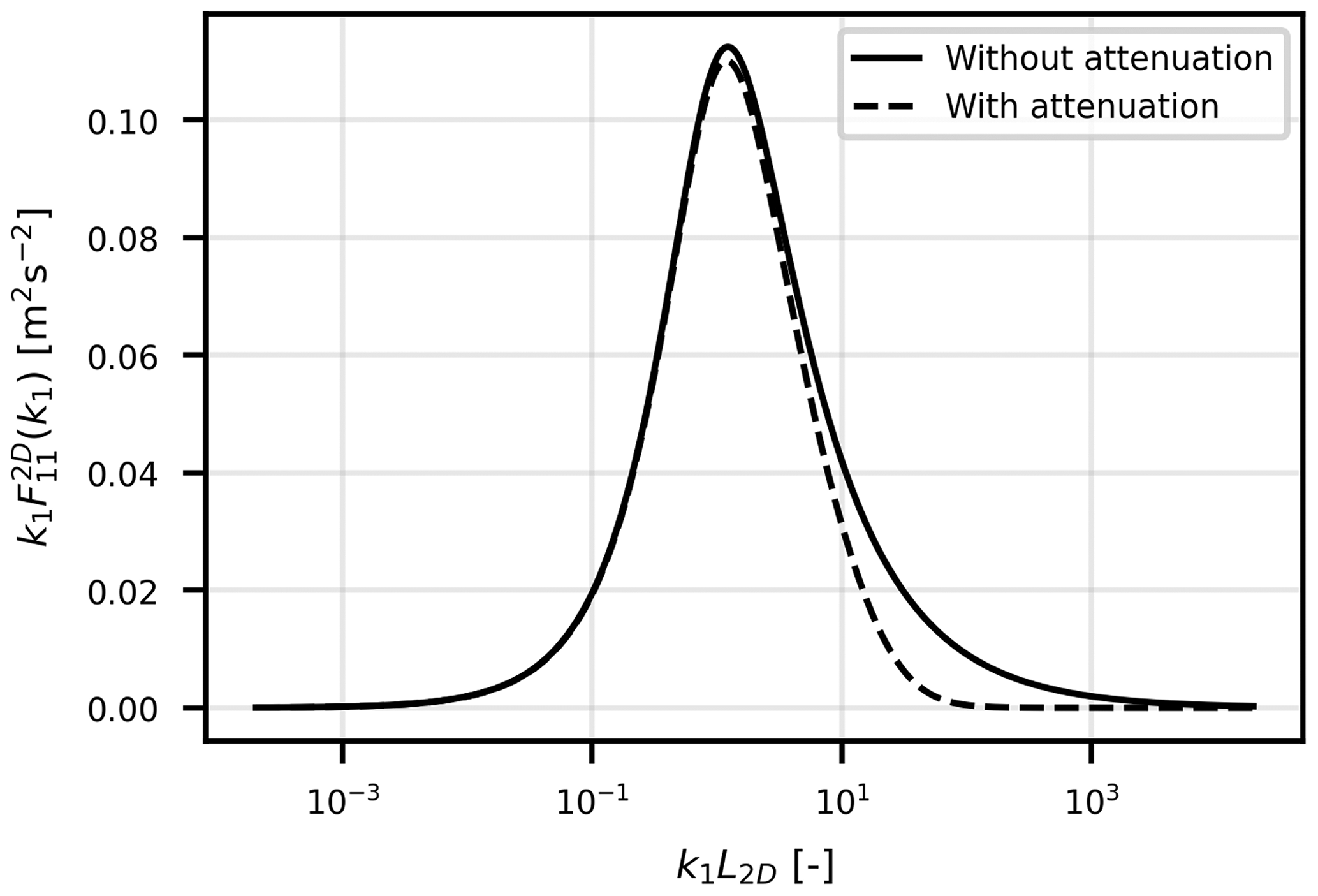
Figure 1 Effect of attenuation at high wavenumbers on F₁₁ spectrum. Here the model parameters are L_2D=20 km, z_i=500 m, and ψ=43°.

It is important to note that although this model utilizes the wavenumber information to generate a spatial field containing large-scale fluctuations, Taylor's frozen turbulence hypothesis can be used to sweep the spatial field into a frequency domain. More intricate models, such as those presented by Wilczek et al. (2015) and de Maré and Mann (2016), characterize spatiotemporal turbulence structures as a function of both wavenumber and frequency. However, for the sake of simplicity, the model presented here disregards the temporal variation or distortion of eddies.

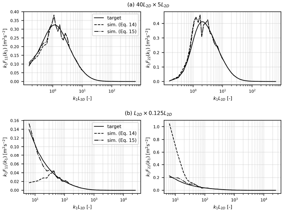
Figure 2 Simulated and target F₁₁ and F₂₂ spectra for 2D rectangular grids having dimensions of (a) 40L_2D×5L_2D and (b) L_2D×0.125L_2D. Solid lines represent the target spectrum, dashed lines represent simulated spectra from C_ij(k) obtained using Eq. (15), and dash–dotted lines represent C_ij(k) obtained using Eq. (16). The simulated spectra are obtained from the mean of 10 realizations. Other parameters are σ²=2 m² s⁻², z_i=500 m, and ψ=45°.

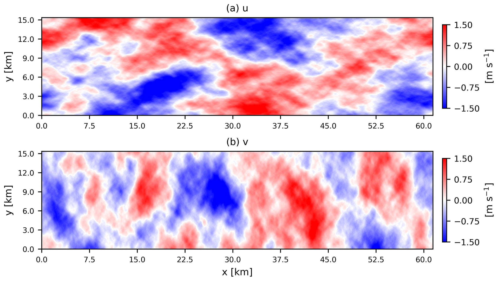
Figure 3 Simulated low-frequency fluctuations in longitudinal u and transverse v wind components. Here the input parameters are L_2D=15 km, σ²=0.6 m² s⁻², z_i=500 m, and ψ=43°.

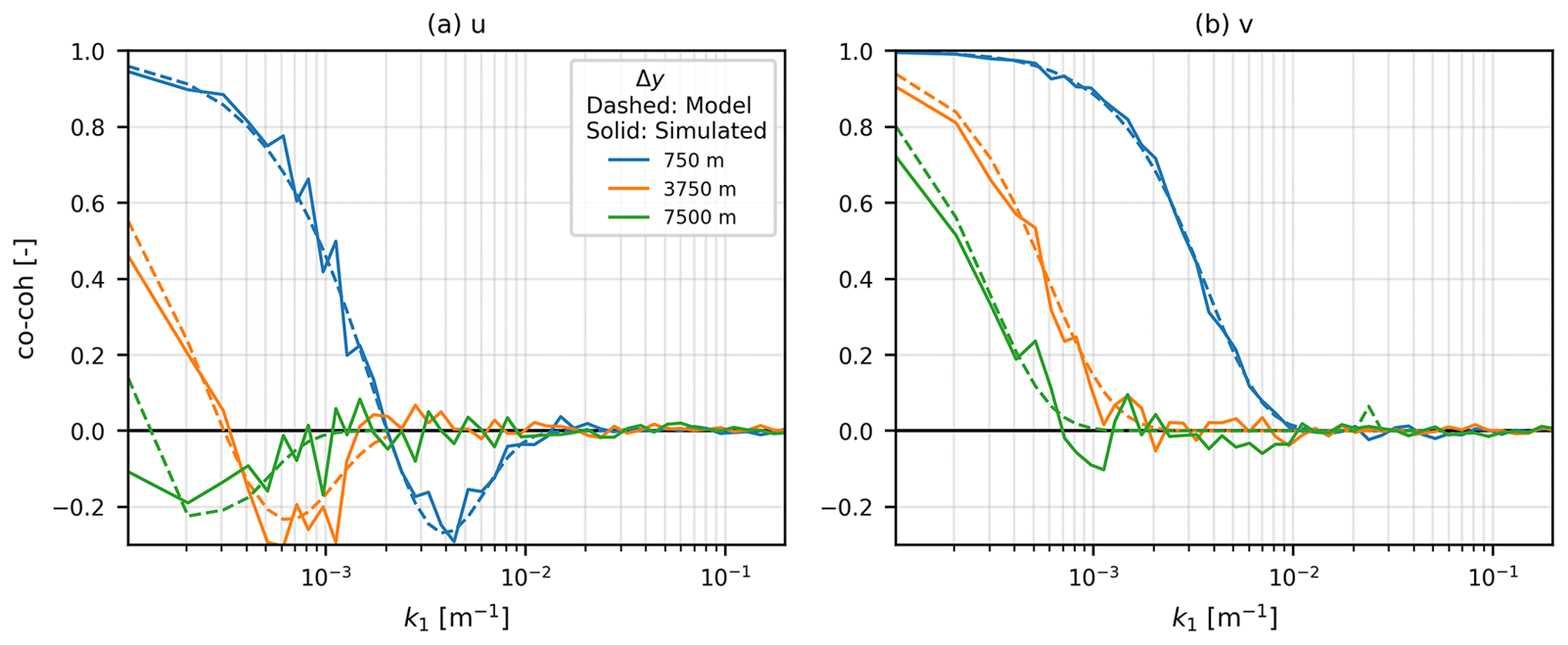
Figure 4 Co-coherence of u and v fluctuations at different Δy separations for the 2D wind field shown in Fig. 3. The dashed curves show theoretical values, and solid curves show simulated values.

The 2D turbulence model (Syed and Mann, 2024) combined with the Mann uniform shear model for 3D turbulence was validated against measurements from two offshore sites: 10 Hz ultrasonic measurements from the FINO1 research platform in the North Sea and line-of-sight (LOS) wind measurements from a forward-looking nacelle lidar in the Hywind Scotland offshore wind farm. The corresponding model parameters that fit the measurements at these two sites can be found in Syed and Mann (2024). A good agreement was recorded between observed and predicted auto-spectra, cross-spectra, and co-coherences. The measured data were classified into different atmospheric stability classes, and it was found that for a 1 h time series, low-frequency fluctuations existed in all stability classes. However, the relative strength of 2D turbulence, compared to 3D turbulence, was more dominant during stable stratification. For the 1 h time series, the mesoscale turbulence peak corresponding to L_2D was also not observed. At both sites, the low-frequency turbulence was in the $F\left(k\right)\propto k_{\mathrm{1}}^{-\mathrm{5}/\mathrm{3}}$ range. For the FINO1 site, the measured value of ψ was close to 45° in the low-frequency range, representing isotropic 2D turbulence. At Hywind Scotland, we observed ψ<40° reflecting the anisotropy in the 2D turbulence.

In summary, the low-frequency turbulence model has four input parameters:

1. ${\mathit{\sigma }}_{\mathrm{2}\mathrm{D}}^{\mathrm{2}}$ the variance exhibited by low-frequency fluctuations (excluding the attenuation);

2. L_2D the length scale corresponding to the peak of mesoscale turbulence;

3. ψ the anisotropy parameter; and

4. z_i the attenuation length, which is assumed to be the boundary-layer height.

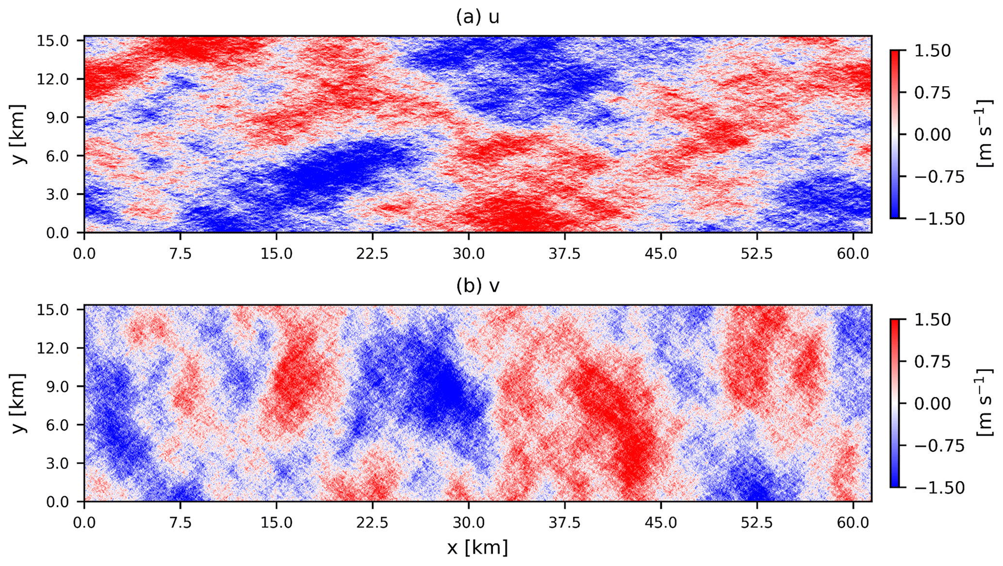
Figure 5 Combined 2D + 3D fluctuations in longitudinal u and transverse v wind components. The 2D turbulence parameters are the same as in Fig. 3. The 3D turbulence parameters are $\mathit{\alpha }{\mathit{ϵ}}^{{}^{\mathrm{2}}/\mathrm{3}}=\mathrm{0.01}$ m${}^{\mathrm{4}/\mathrm{3}}$ s⁻², L_3D=50 m, and Γ=2.5.

Figure 6 Same as Fig. 5 but a vertical slice of combined 2D + 3D fluctuations.

3 2D wind field simulation

Here, we follow the procedure of Mann (1998) to simulate low-frequency, anisotropic wind fields. The 2D turbulence is assumed to be statistically homogeneous in horizontal directions and constant in the vertical direction. Taylor's frozen turbulence hypothesis is also employed to convert the wavenumber domain into the frequency domain. The wind field will be simulated on a horizontal grid with N₁ and N₂ grid points in the longitudinal and transverse directions, respectively. The length of the grid in two directions would be $L_{\mathrm{1}}=N_{\mathrm{1}}\cdot \mathrm{d}x$ and $L_{\mathrm{2}}=N_{\mathrm{2}}\cdot \mathrm{d}y$. Following Mann (1998), the incompressible, homogeneous, 2D velocity field can be written as a sum of discrete Fourier modes:

$$\begin{array}{}\text{(12)}& u_i\left(\mathit{x}\right)=\sum _{\mathit{k}}\exp (\mathit{\iota }\mathit{k}\mathbf{\cdot }\mathit{x})C_{ij}\left(\mathit{k}\right)n_j\left(\mathit{k}\right),\end{array}$$

where ∑_k denotes the sum over all wave vectors k, where $k_i=m\mathrm{2}\mathit{\pi }/L_i$ for $m=-N_i/\mathrm{2},\mathrm{\dots },N_i/\mathrm{2}$. C_ij(k) are the Fourier coefficients, and n_j(k) are independent Gaussian stochastic variables. Here, the summation over repeated indices is assumed. The solution to Eq. (12) is approximately

$$\begin{array}{}\text{(13)}& C_{ij}\left(\mathit{k}\right)n_j\left(\mathit{k}\right)={\displaystyle \frac{\mathrm{1}}{L_{\mathrm{1}}{L}_{\mathrm{2}}}}\underset{A}{\int }{u}_i\left(\mathit{x}\right)\exp (-\mathit{\iota }\mathit{k}\mathbf{\cdot }\mathit{x})\mathrm{d}\mathit{x},\end{array}$$

where ∫_Adx is integration over the area L₁×L₂. The process of obtaining C_ij involves multiplying Eq. (13) with its complex conjugate, which gives

$$\begin{array}{}\text{(14)}& C_{ij}^{*}\left(\mathit{k}\right)C_{ij}\left(\mathit{k}\right)=\int {\mathit{\varphi }}_{ij}\left({\mathit{k}}^{\mathbf{\prime }}\right)\prod _{(l=\mathrm{1})}^{\mathrm{2}}{\text{sinc}}^{\mathrm{2}}\left({\displaystyle \frac{(k_l-k_l^{\prime })L_l}{\mathrm{2}}}\right)\mathrm{d}{\mathit{k}}^{\mathbf{\prime }},\end{array}$$

where $\text{sinc}x\equiv \left(\sin x\right)/x$. In the case if L_l≫L_2D, where $l=\mathrm{1},\mathrm{2}$, Eq. (14) can be simplified to

$$\begin{array}{}\text{(15)}& C_{ij}^{*}\left(\mathit{k}\right)C_{ij}\left(\mathit{k}\right)={\displaystyle \frac{(\mathrm{2}\mathit{\pi }{)}^{\mathrm{2}}}{L_{\mathrm{1}}{L}_{\mathrm{2}}}}{\mathit{\varphi }}_{ij}\left(\mathit{k}\right).\end{array}$$

The length scale L_2D corresponding to the mesoscale turbulence peak is quite large, usually on the order of 10⁵ to 10⁶ m. Simulating a high-resolution wind field containing the wavenumbers corresponding to L_2D would be costly in terms of computation time. Usually, L₂≪L_2D when simulating wind fields for single wind turbine load calculations. So, the simplified relation in Eq. (15) no longer holds true. We have observed that if we simplify the sinc² function for L₁ and replace it with $\mathrm{2}\mathit{\pi }/L_{\mathrm{1}}$ but integrate the sinc² function for L₂, we would get simulated spectra much closer to the target spectra.

$$\begin{array}{}\text{(16)}& C_{ij}^{*}\left(\mathit{k}\right)C_{ij}\left(\mathit{k}\right)={\displaystyle \frac{\mathrm{2}\mathit{\pi }}{L_{\mathrm{1}}}}\int {\mathit{\varphi }}_{ij}(k_{\mathrm{1}},k_{\mathrm{2}}^{\prime }){\text{sinc}}^{\mathrm{2}}\left({\displaystyle \frac{(k_{\mathrm{2}}-k_{\mathrm{2}}^{\prime })L_{\mathrm{2}}}{\mathrm{2}}}\right)\mathrm{d}{k}_{\mathrm{2}}^{\prime }\end{array}$$

To speed up the numerical integration, the limits of integration are $k_{\mathrm{2}}-\mathrm{2}\mathit{\pi }/L_{\mathrm{2}}$ to $k_{\mathrm{2}}+\mathrm{2}\mathit{\pi }/L_{\mathrm{2}}$. A correction factor is multiplied, compensating for the loss in variance due to the limited integration interval. This problem with discretization has been discussed in detail by Mann (1998). The Fourier coefficients obtained from Eq. (15) or Eq. (16) after taking a matrix square root are then multiplied by a random Gaussian field. The resulting product's inverse discrete Fourier transform would yield the wind field.

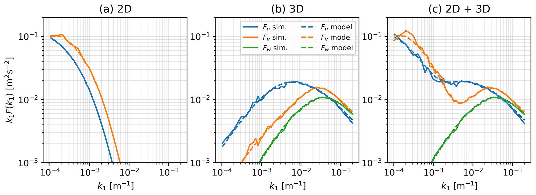
Figure 7 Spectra of 2D, 3D, and combined 2D + 3D fluctuations in longitudinal u and transverse v wind components. Solid lines present the simulated spectra, and dashed lines reflect the theoretical spectra. The w spectra for 3D turbulence are also shown.

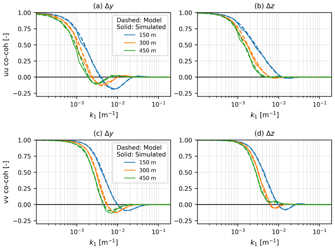
Figure 8 The u and v co-coherences at different Δy and Δz values for combined 2D + 3D fluctuations. The dashed curves show theoretical values, and solid curves show simulated values.

Figure 2 illustrates the effect of discretization on the simulated spectra. In Fig. 2b when L₂≪L_2D, C_ij(k) obtained via Eq. (15) underestimate F₁₁(k₁) and overestimate F₂₂(k₁) at very low k₁ values. In such cases, C_ij(k) must be evaluated using Eq. (16).

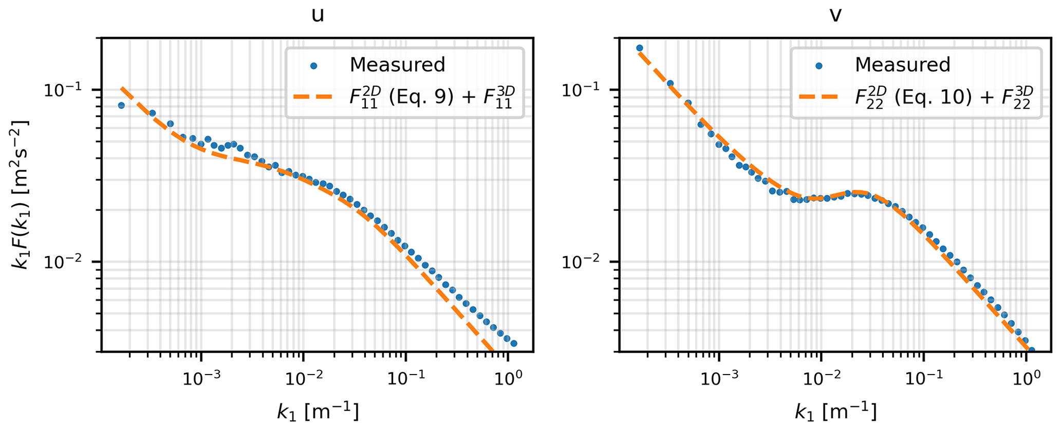
Figure 3 shows the simulated u and v low-frequency fluctuations, where the input parameters are L_2D=15 km, σ²=0.6 m² s⁻², z_i=500 m, and ψ=43°. These parameters, with the exception of L_2D, are representative of typical neutral conditions for $\mathrm{8}<\stackrel{\mathrm{‾}}{U}<$10 ms⁻¹ at the FINO1 offshore site. Here, large-scale coherent structures can be identified along the longitudinal axis for the u component. We can also observe the almost equal variance in the u and v fluctuations due to ψ being close to the isotropic value of 45°. The one-dimensional (1D) spectra of this simulated 2D wind field are illustrated in Fig. 7a. The spectra derived from the simulated wind field are in excellent agreement with the theoretical spectra mentioned in Eqs. (10) and (11). Normalized cross-spectra (co-coherence, the real part of the cross-spectrum divided by the auto-spectrum) for the simulated 2D wind field components are also compared with the theoretical expression in Eq. (6). In Fig. 4, co-coherence of u and v is plotted as a function of k₁ for separations ranging from 750 to 7500 m. Once the lateral separation distance Δy approaches L_2D (in this case 15 km), the normalized cross-spectra decrease significantly.

4 Combining 2D and 3D fluctuations

Mann (1994) presented the uniform shear model for small-scale turbulence in the neutral atmosphere. We combine the two models, assuming that the large-scale and small-scale fluctuations are independent. Combining the mesoscale and microscale turbulence in the frequency or wavenumber domain requires an assumption of weak or no correlation between the two scales. Högström et al. (2002) provided a qualitative framework for combining the spectra at large and small scales in the atmosphere by a simple superposition method. On a similar pattern, Kim and Adrian (1999) noted that the 1D spectrum of streamwise velocity in a turbulent pipe flow has a bimodal representation of high- and low-wavenumber modes. These two modes are associated with small- and large-scale turbulent motions, respectively. Superposing these two modes gives a good general representation of the measured spectra over the whole wavenumber domain since the two modes are uncorrelated.

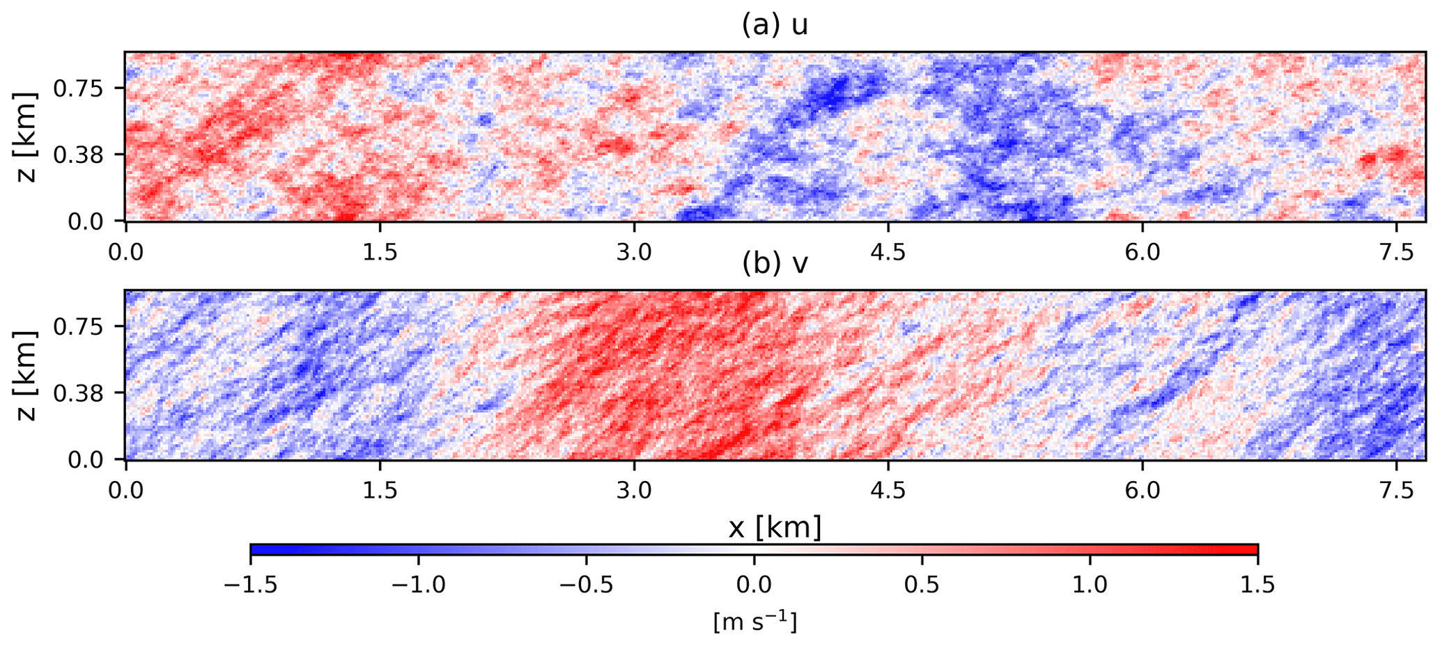
Figure 5 displays a 2D + 3D turbulence wind field of u and v wind components for relatively smaller dimensions. The 3D wind field is generated by the Mann uniform shear turbulence model, which has three input parameters: the dissipation parameter $\mathit{\alpha }{\mathit{ϵ}}^{\mathrm{2}/\mathrm{3}}=\mathrm{0.01}$ m${}^{\mathrm{4}/\mathrm{3}}$ s⁻², the turbulence length scale L_3D=50 m, and the anisotropy parameter Γ=2.5. The values of the parameters selected here are typical of offshore wind conditions at the FINO1 site for neutral conditions (Syed and Mann, 2024). The 3D turbulent wind field is also generated by the procedure presented in Mann (1998). Since the wind fields are assumed statistically independent, they can be added to get the combined fluctuations. In this case, the 2D wind field components are directly added to all the vertical planes of the corresponding 3D turbulence box. We can observe the increased variance in the combined 2D and 3D wind fluctuations. The large-scale coherent structures are still dominant, but we now also observe smaller structures. A smaller vertical slice of the same wind field is illustrated in Fig. 6. Here, one can observe the large shear in the v component compared to the u component. This implies that the phase difference between v fluctuations at different heights is higher (φ_v>φ_u), as observed in atmospheric turbulence measurements at multiple sites (Chougule et al., 2012; Syed and Mann, 2024). The 1D two-sided spectra of the 3D turbulence wind field by itself and combined with the low-frequency fluctuations are shown in Fig. 7b and c, respectively. The resulting spectra add individual 2D and 3D wind field spectra over the wavenumber domain.

The u and v co-coherences of simulated combined 2D + 3D wind field at different lateral and vertical separations are illustrated in Fig. 8. The co-coherences are plotted for lateral and vertical separations ranging from 150 to 450 m. At lower k values, the low-frequency fluctuations are fully coherent for all vertical Δz separations, and we obtain co-coherence values close to 1. This is because the low-frequency fluctuations are assumed to be constant in the vertical direction at any instant. The same can not be said about the lateral Δy separations, as we have observed a decrease in the u co-coherence of low-frequency fluctuations for increasing lateral separations in Fig. 8a.

5 Discussion

5.1 The effect of anisotropy parameter on 2D turbulence

As mentioned earlier, ψ=45° represents isotropic 2D wind fields. Altering the ψ parameter by decreasing or increasing it from 45° leads to the elongation of significant coherent structures, extending them longitudinally and laterally, respectively. The effect of changing the anisotropy parameter ψ can be observed in Fig. 9. Here u and v fluctuations are shown on a 15 km × 15 km grid for different values of ψ. Figure 9a shows the u and v fluctuations for ψ=20°, and we can observe the large-scale coherent structures in the longitudinal direction. These structures exhibit significantly larger values of fluctuations, i.e., ${\mathit{\sigma }}_u^{\mathrm{2}}>{\mathit{\sigma }}_v^{\mathrm{2}}$. Figure 9b illustrates the isotropic case when both u and v fluctuations have similar strength and ${\mathit{\sigma }}_u^{\mathrm{2}}={\mathit{\sigma }}_v^{\mathrm{2}}$. By increasing the value of ψ to 70° (Fig. 9c), the large-scale coherent structures in the lateral direction get stretched, and we also observe ${\mathit{\sigma }}_u^{\mathrm{2}}<{\mathit{\sigma }}_v^{\mathrm{2}}$.

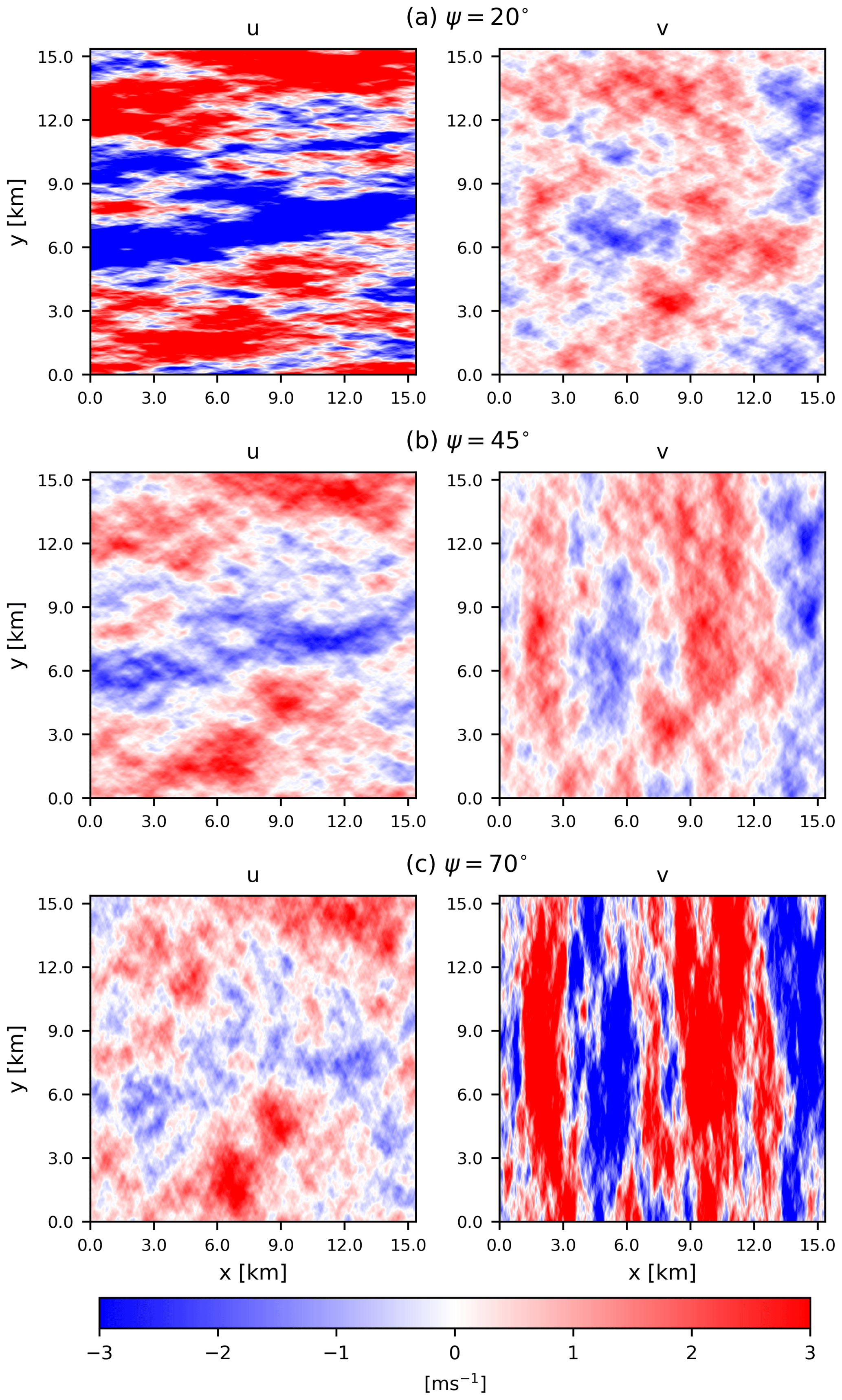
Figure 9 Effect of anisotropy parameter ψ on the wind field: (a) ψ=20°, (b) ψ=45° (isotropic turbulence), and (c) ψ=70°. Here the other input parameters are L_2D=5 km, σ²=1 m² s⁻², and z_i=100 m.

Figure 10 An example of theoretical spectra plotted over measured spectra obtained from FINO1 at z=81 m and $\stackrel{\mathrm{‾}}{U}=\mathrm{10}$ ms⁻¹. Equations (10) and (11) are plotted with L_2D=150 km and z_i=100 m.

Figure 11 An example of periodicity in 2D wind field simulations.

The length scales of the two velocity components can be determined by identifying the maximum of $k_i{F}_{ii}^{\mathrm{2}\mathrm{D}}\left(k_i\right)$ for $i=\mathrm{1},\mathrm{2}$. Let $L_{i,k_i}\equiv \mathrm{1}/k_{\max ,i}$, where k_max,i denotes the wavenumber at the peak of $k_i{F}_{ii}^{\mathrm{2}\mathrm{D}}\left(k_i\right)$. These length scales can be computed numerically. At ψ=45°, the ratio $L_{u,k_{\mathrm{1}}}/L_{v,k_{\mathrm{2}}}$ equals 1, indicating that the length scales of u and v are equivalent in the k₁ and k₂ directions, respectively. When ψ<45°, turbulence structures elongate in the longitudinal direction, resulting in $L_{u,k_{\mathrm{1}}}/L_{v,k_{\mathrm{2}}}>\mathrm{1}$. Conversely, for ψ>45°, the inverse holds true. Moreover, the ratios $L_{u,k_{\mathrm{1}}}/L_{v,k_{\mathrm{1}}}$ and $L_{v,k_{\mathrm{2}}}/L_{u,k_{\mathrm{2}}}$ are independent of the anisotropy parameter. It is noted that these length-scale ratios are approximately equal to $\sqrt{\mathrm{3}}$, or about 1.73.

5.2 Guidelines for simulating 2D wind fields

Usually ${\mathit{\sigma }}_{\mathrm{2}\mathrm{D}}^{\mathrm{2}}$ and ψ are obtainable at a specific site through fitting Eqs. (10) and (11) to the measured spectra. For z_i, some advanced measurements like ground-based remote sensing tools such as a ceilometer can be used or obtained through reanalysis data sets or simply estimated. To obtain L_2D through measurements, we would need a time series spanning from 10 d to 1 month (see Fig. 3 in Larsén et al., 2016). This suggests L_2D to be on the order of 10⁵–10⁶ m. Such extremely low frequencies corresponding to L_2D are not interesting for the wind turbine design process. For fitting Eqs. (10) and (11) to the measured spectra we can assume L_2D→∞. But for wind field simulation purposes, this is not realistic since it would lead to ${\mathit{\sigma }}_{\mathrm{2}\mathrm{D}}^{\mathrm{2}}\to \mathrm{\infty }$. For load estimation on wind turbine structures, a 1 h time series is usually sufficient for estimating the impact of low-frequency fluctuations. Hence, an arbitrarily high value of L_2D can be used to simulate low-frequency wind fluctuations. An example of this is shown in Fig. 10 where a value of L_2D=150 km is used to plot the theoretical spectra in Eqs. (10) and (11) over the u and v spectra measured at the FINO1 test site.

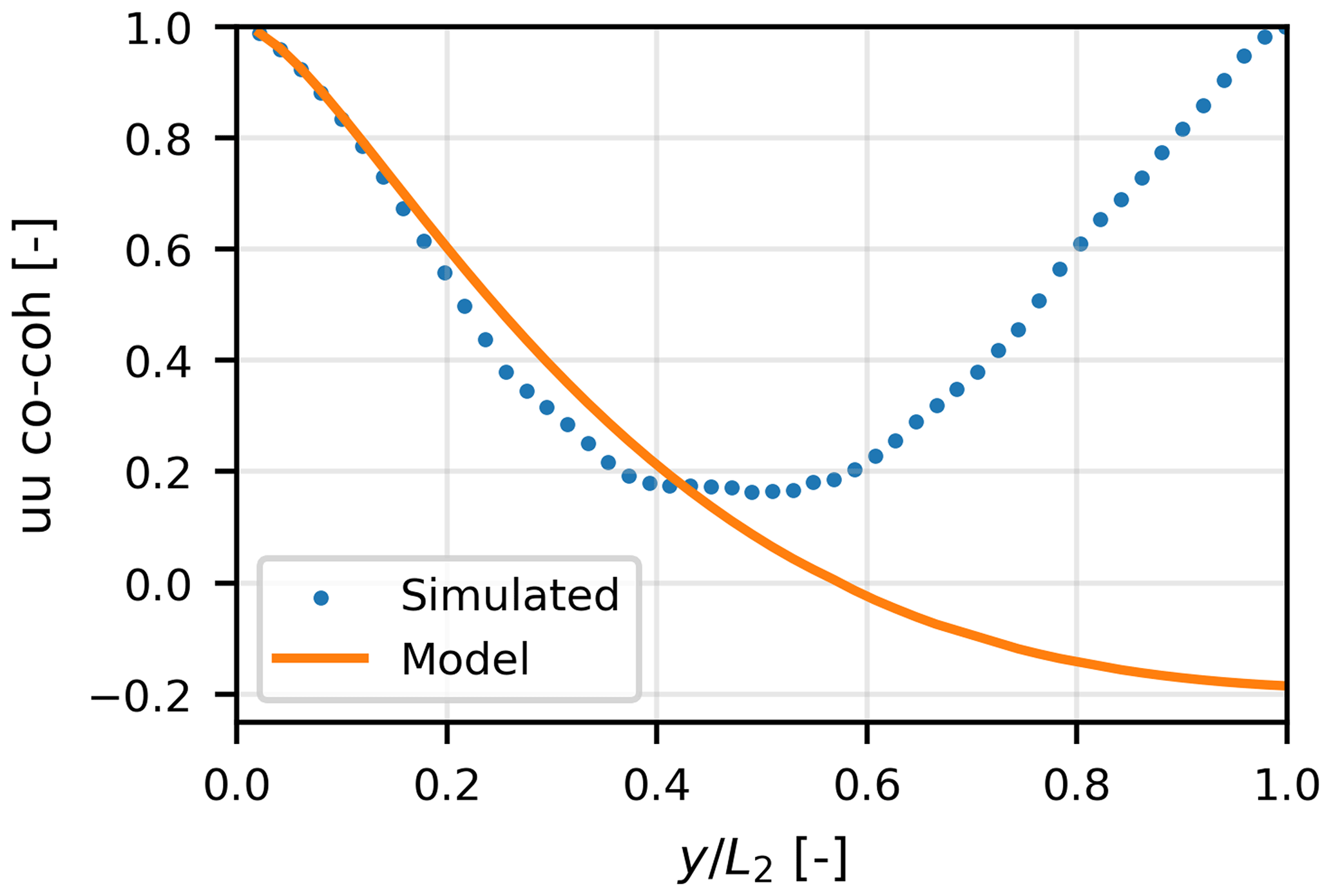
An unwanted effect of the simulation method presented here is the periodicity in wind fluctuations, which was also discussed by Mann (1998). The periodicity implies that wind fluctuations at grid points on either side of the box j and $N_{\mathrm{2}}-j+\mathrm{1}$ for small j are coherent. This behavior is shown in Fig. 11 where co-coherence of u fluctuations is plotted as a function of lateral distance. It can be observed that both the simulated and model co-coherence values decrease when y approaches $L_{\mathrm{2}}/\mathrm{2}$. Due to periodicity, the simulated co-coherence increases for $y>L_{\mathrm{2}}/\mathrm{2}$. The solution to this problem is choosing L₂ to be at least twice the characteristic length of the structure under analysis. In the case of wind turbines, L₂ should be at least greater than twice the rotor diameter of the wind turbine. A good practice is to simulate the low-frequency fluctuations on a much larger grid than the high-frequency fluctuations. To combine the 2D and 3D turbulence, a smaller section of the 2D wind field, equal in length and grid points to the 3D turbulence plane, is added to all the vertical levels of the 3D turbulence box.

6 Conclusions

A method to generate the low-frequency wind fluctuations is introduced. This method utilizes the spectral tensor presented by Syed and Mann (2024) to generate 2D stochastic wind fields for the longitudinal u and lateral v wind components. The generated wind fields contain large-scale and low-frequency wind fluctuations called 2D turbulence. The model employs four input parameters: (i) the variance characterizing low-frequency fluctuations ${\mathit{\sigma }}_{\mathrm{2}\mathrm{D}}^{\mathrm{2}}$, (ii) a length scale corresponding to large-scale flow structures L_2D, (iii) an anisotropy parameter ψ, and (iv) a cutoff or attenuation length z_i. The simulation method uses the wind field presented as a discrete Fourier series, where Fourier coefficients are derived from the 2D spectral model. The coefficients are then multiplied by a random Gaussian field. Subsequently, the product's inverse discrete Fourier transform yields a 2D wind field featuring low-frequency, anisotropic wind fluctuations. Issues arising from the discretization, such as underestimation of the spectral density at very low wavenumbers and periodicity, are also addressed in this study. Some guidelines to simulate the wind fields containing 2D turbulence are also provided in the context of wind energy applications.

The 2D turbulence wind field can be added to a 3D turbulence field to get the spectral representation over a wide frequency range. We combined the 2D turbulence wind field with a 3D turbulence field generated using the Mann uniform shear turbulence model. The spectra and co-coherences from the combined simulated 2D + 3D turbulence wind are compared with the theoretical expressions, and an excellent agreement was observed. The 2D turbulence simulation program is open-source and can be accessed via the link in the “Code availability” section.