Machine-learning-based estimate of the wind speed over complex terrain using the long short-term memory (LSTM) recurrent neural network

Accurate estimation of the wind speed profile is crucial for a range of activities such as wind energy and aviation. The power law and the logarithmic-based profiles have been widely used as universal formulas to extrapolate the wind speed profile. However, these traditional methods have limitations in capturing the complexity of the wind flow, mainly over complex terrain. In recent years, the machine-learning techniques have emerged as a promising tool for estimating the wind speed profiles. In this study, we used the long short-term memory (LSTM) recurrent neural network and observational lidar datasets from three different sites over complex terrain to estimate the wind profile up to 230 m. Our results showed that the LSTM outperformed the power law as the distance from the surface increased. The coefficient of determination (R²) was greater than 90 % up to 100 m for input variables up to a 40 m height only. However, the performance of the model improved when the 60 m wind speed was added to the input dataset. Furthermore, we found that the LSTM model trained on one site with 40 and 60 m observational data and when applied to other sites also outperformed the power law. Our results show that the machine-learning techniques, particularly LSTM, are a promising tool for accurately estimating the wind speed profiles over complex terrain, even for short observational campaigns.

1 Introduction

Machine-learning techniques are increasingly being adopted as powerful tools in environmental sciences. We see many examples of this method applied for different purposes to forecast meteorological variables and their derivative products (Musyimi et al., 2022; Jiang et al., 2022; Mustakim et al., 2022; Jesemann et al., 2022). However, the use of the machine-learning techniques is not restricted to the local or regional scales. Liu et al. (2022), for example, proposed a multi-level circulation pattern classification to identify large-scale weather or climate disaster events. The forecasting and monitoring disasters were also the subject of Soria-Ruiz et al. (2022). They got high performance by applying machine-learning algorithms to remote sensing datasets to detect the recurrent floods over the Gulf of Mexico coastline and the central and southeastern part of Mexico. Among the methods evaluated, Song and Wang (2020) concluded that the neural networks are superior to produce monthly wildfire predictions 1 year in advance, providing thus a valuable information for long-range fire planning and management. Adding the principal component analysis (PCA), Zhang et al. (2022) improved the accuracy for the visibility prediction at Sichuan (China). Among the six machine-learning algorithms evaluated, they found that the neural network performed best. Cheng and Tsai (2022) proposed a hybrid methodology based on variable selection and autoregressive distributed lag to forecast the pollutant concentrations, which improved the results when compared to the full and without-lag dataset. The support vector regression (SVR), which is a supervised algorithm, performed better than the other four algorithms tested. Those are only a few examples of innovative works adopting the machine-learning techniques in the environmental sciences.

Wind forecasts underpin wind power prediction, which is essential to support wind energy production in the short term. Although winds have been traditionally forecasted with numerical weather prediction models, the use of machine learning has become more widespread not only to correct the biases derived from the highly variable nature of the winds, but also as stand-alone prediction models. Wang et al. (2021) showed that their multi-layer cooperative combined forecasting system, which is based on a novel adaptive weighting scheme, overcame the limitations of the current single and combined forecasting methods and provided a more accurate and stable forecast. In their review paper, Bali et al. (2019) analyzed a few studies produced during this century and concluded that the techniques for the wind speed forecast have limitations, such as low efficiency and high computational cost. They proposed the use of long short-term memory (LSTM) to improve wind speed forecasting for power prediction. Tukur et al. (2022) analyzed works produced between 2010 and 2020 and concluded that ensemble and hybrid methods achieve high accuracy because they present more abilities to model complex functions than the linear models. They agreed with Bali et al. (2019) that the LSTM looks promising in forecasting the wind speed whilst recommending further investigation on the capabilities of hybrid model approaches. Dalton and Bekker (2022) showed the improvement when considering other meteorological variables in the modeling. Their results pointed to the vertical wind and divergence as important predictors to the wind speed. In this way, He et al. (2022) included the 2 m temperature and surface pressure to train their dual-attention mechanism multi-channel convolutional LSTM model with the ERA5 dataset to forecast the 10 m wind speed. Zhou et al. (2023) also used the ERA5 dataset to investigate the grid-to-site conversion models, considering altitude, land use and seasonality effects. The deep learning models outperformed the linear interpolation and the regression models to estimate the 10 m wind speed. The aforementioned works briefly exemplify that efforts have been made with the wind speed forecast theme; however, the methods to estimate its vertical profile are still limited.

According to Pintor et al. (2022), extrapolating the wind speed to higher heights is still a challenge, and of the two most widely used methods (the power law and the logarithmic-based profile) they found that the power law is more accurate for a wide variety of landscapes. The Met Office (United Kingdom) developed the Virtual Met Mast (VMM) tool (Standen et al., 2016) to assess the wind profile; however, this technique requires high-spatial-resolution weather numerical prediction (Schwegmann et al., 2023). Only recently have machine-learning techniques been used to forecast the wind speed profile. Türkan et al. (2016) evaluated seven different machine-learning methods to estimate the 30 m wind speed at Kütahya (Türkiye) and concluded that the SVR produced the most realistic results compared to the other six. Al-Shaikhi et al. (2022) proposed the particle swarm optimization (PSO) with the LSTM method and compared their results with other optimization algorithms for an experiment carried out at Dhahran (Saudi Arabia). Their model needs at least four different levels of observational data as input. Similarly, Nuha et al. (2022) proposed the regularized extreme learning machine (RELM) to extrapolate the wind speed to higher heights. With the same dataset of Dhahran, Mohandes and Rehman (2018) used the restricted Boltzmann machine (RBM) method and observations at four different heights as input. They showed that their method improved the wind speed forecast. Bodini and Optis (2020a) and Bodini and Optis (2020b) found that random forests outperform standard wind extrapolation approaches, using a round-robin validation method. They highlighted the benefits of including observational data capturing the diurnal variability of the atmospheric boundary layer, namely the Obukhov length, turbulence kinetic energy and time of the day, all of them measured at a 4 m height. Vassallo et al. (2020) also improved their results, including meteorological variables in the input dataset of their artificial neural network (ANN) model, advising to carefully select the input data and emphasizing the importance of normalization. Even the VMM data are improved with machine-learning methods (Schwegmann et al., 2023). Bodini and Optis (2020a) and Bodini and Optis (2020b) conducted their experiments over low-complexity terrain (Great Plains – US) and stressed the need of performing the same kind of analysis in more complex terrains. To the best of our knowledge, most studies on vertical wind speed extrapolation were conducted for low-complexity orographies, except for Vassallo et al. (2020), who analyzed different types of terrain complexity, and Standen et al. (2016) and Schwegmann et al. (2023), who conducted their studies through the VMM tool.

2 Data and methods

2.1 The LSTM recurrent neural network

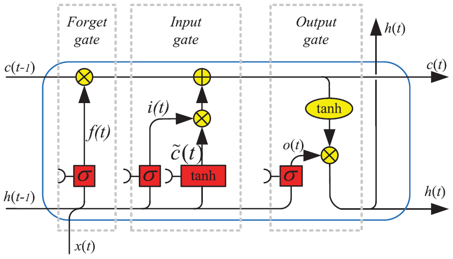
Recurrent neural networks (RNNs) are a type of artificial neural network where the output of one time step is used as an input in the subsequent time step to then build a memory of time series events. The RNNs are specifically designed to work, learn and predict sequential data (Medsker and Jain, 1999). Long short-term memory (LSTM) is a type of RNN that is considered a state-of-the-art tool for processing sequential and temporal data nowadays. The main advantage of the LSTM over the other RNNs is that the presence of internal memory allows maintaining long-term dependencies, avoiding the vanishing- or exploding-gradient problems (Smagulova and James, 2019). This was done by introducing a forget gate into the standard recurrent sigma cell of the RNNs. The forget gate can decide what information will be discarded (Yu et al., 2019) and makes the LSTM system a robust model that compensates for the imperfections in the input data (Sherstinsky, 2020). The LSTM cells are mathematically expressed by

$$\begin{array}{}\text{(1)}& {\displaystyle }& {\displaystyle }{f}_t=\mathit{\sigma }\left(W_{fh}{h}_{t-\mathrm{1}}+W_{fx}{x}_t+b_f\right),\text{(2)}& {\displaystyle }& {\displaystyle }{i}_t=\mathit{\sigma }\left(W_{ih}{h}_{t-\mathrm{1}}+W_{ix}{x}_t+b_i\right),\text{(3)}& {\displaystyle }& {\displaystyle }{\stackrel{\mathrm{̃}}{c}}_t=\tanh \left(W_{\stackrel{\mathrm{̃}}{c}h}{h}_{t-\mathrm{1}}+W_{\stackrel{\mathrm{̃}}{c}x}{x}_t+b_{\stackrel{\mathrm{̃}}{c}}\right),\text{(4)}& {\displaystyle }& {\displaystyle }{c}_t=f_t\cdot c_{t-\mathrm{1}}+i_t\cdot {\stackrel{\mathrm{̃}}{c}}_t,\text{(5)}& {\displaystyle }& {\displaystyle }{o}_t=\mathit{\sigma }\left(W_{oh}{h}_{t-\mathrm{1}}+W_{ox}{x}_t+b_o\right),\text{(6)}& {\displaystyle }& {\displaystyle }{h}_t={\mathit{\sigma }}_t\tanh \left(c_t\right),\end{array}$$

where x_t and h_t are the inputs and the recurrent information at time t; c_t is the cell state of the LSTM; f_t, i_t and o_t are the forget, input and output gates; W_f, W_i, $W_{\stackrel{\mathrm{̃}}{c}}$ and W_o are the weights; b is the bias; and the operator “⋅” is the pointwise multiplication of two vectors. Figure 1 illustrates the LSTM compounds and architecture.

Figure 1 LSTM schematical diagram (Yu et al., 2019).

We run the LSTM using the Keras library (version 2.9) from Python (version 3.8.16) through Colab (the Google Research platform). The missing data were interpolated using the interpolate Pandas function through a linear method. Afterwards, the data were normalized through the StandardScaler function from the Sklearn library (Pedregosa et al., 2011). The StandardScaler function normalizes by removing the mean and scaling to the standard deviation:

$$\begin{array}{}\text{(7)}& z=(x-u)/s,\end{array}$$

where x is observed data, u is the mean, s is the standard deviation and z is the normalized data.

We identified the optimal hyperparameters by using the KerasTuner (O'Malley et al., 2019) with the Hyperband algorithm. Table A1 exhibits the tuned hyperparameters for each experiment. We maintained the default configuration of Keras for the other LSTM arguments (Keras, 2023). See Table A2.

2.2 Doppler lidar

We employed the Windcube v2 Doppler lidar, from Leosphere, during the field campaigns at three different sites. For the Windcube v2 technical specifications, see Beu and Landulfo (2022). The information of the field campaigns is listed in Table 1.

Table 1 Information of the field campaigns.

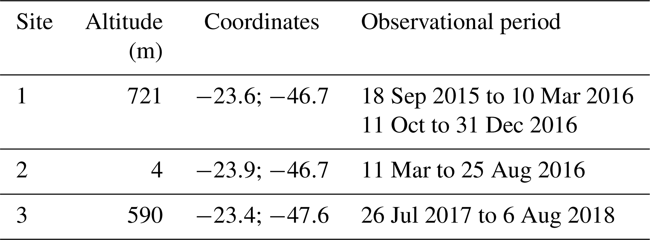
The lidar was set up for 12 levels, as follows: 40, 60, 80, 100, 120, 140, 160, 180, 200, 230, 260 and 290 m; it was also set up to retrieve information every 10 min. The Windcube v2 system automatically discards data when the carrier-to-noise (CNR) ratio is under −23 dB, and we removed data that presented availability less than 80 % over 10 min.

See in Table A3 that the data availability is over 99 % for all the three sites up to a 160 m height. Above 160 m, the availability decreases to 98 % at Site 2 and 94 % at Site 3 at a 230 m height.

We considered the observed data at 40 m to estimate the wind speed at higher heights (from 60 up to 230 m). Beyond the 10 min mean wind speed (v40), we also considered the wind direction (dir40), the hour, and the standard deviation of the horizontal (σ_u+σ_v) and vertical (σ_w) wind speed to forecast the wind speed at higher heights. With the wind speed standard deviation, we estimated the turbulence kinetic energy (TKE), which is the sum of the wind speed variances (Stull, 1988) and is expressed by

$$\begin{array}{}\text{(8)}& \mathrm{TKE}={\displaystyle \frac{\mathrm{1}}{\mathrm{2}}}\left({\mathit{\sigma }}_u^{\mathrm{2}}+{\mathit{\sigma }}_v^{\mathrm{2}}+{\mathit{\sigma }}_w^{\mathrm{2}}\right).\end{array}$$

As already discovered, including cyclical variables improves the wind speed forecast (Bodini and Optis, 2020a, b; Baquero et al., 2022). The diurnal cycle is a strong feature of the sites under research, and we will discuss this further. Since surface observations are not available, the 40 m TKE could indirectly transmit information related to temperature and stability, improving the modeling with respect to diurnal variability. This step is referred to as Experiment 1. Afterwards, we also added the 60 m wind speed as input to forecast the heights above, and this step is referred to as Experiment 2. Following the advice of Bodini and Optis (2020a) and Bodini and Optis (2020b), we conducted two more experiments (Experiment 3 and Experiment 4), which consisted in swapping a trained model for another environment and evaluating its performance. In this way, the trained model for Site 1 was applied to Sites 2 and 3. In addition, the trained model for Site 2 was applied to Sites 1 and 3, and the trained model for Site 3 was used for Sites 1 and 2. In Table A4, we summarize the input variables of each experiment.

2.3 The power law

According to Pintor et al. (2022), the power law (PL) is the simplest and generally the most effective way to extrapolate the wind speed. The PL is given by

$$\begin{array}{}\text{(9)}& V=V_{\mathrm{r}}{\left({\displaystyle \frac{z}{z_{\mathrm{r}}}}\right)}^{\mathit{\alpha }},\end{array}$$

where V and V_r are the wind speed at height z and at reference height z_r, respectively. α is the wind shear coefficient. The authors state that α<0.1 corresponds to unstable conditions, $\mathrm{0.1}<\mathit{\alpha }<\mathrm{0.2}$ is typical of the neutral profile and α>0.2 describes a stable atmosphere.

2.4 Evaluation

For evaluating the model performances, we chose verification metrics like those used in Zhou et al. (2022) and Baquero et al. (2022), because those metrics have been largely applied to wind forecast through machine-learning methods. For further information on these metrics, see Zhou et al. (2022) and Baquero et al. (2022).

• Coefficient of determination (R²): the R² tells us how much the model differs from the original data, and it is related to the correlation coefficient.

  $$\begin{array}{}\text{(10)}& R^{\mathrm{2}}=\mathrm{1}-{\displaystyle \frac{{\mathrm{\Sigma }}_{i=\mathrm{1}}^N{\left(y_i-\widehat{y_i}\right)}^{\mathrm{2}}}{{\mathrm{\Sigma }}_{i=\mathrm{1}}^N{\left(y_i-\stackrel{\mathrm{‾}}{y}\right)}^{\mathrm{2}}}}\end{array}$$

• Mean squared error (MSE):

  $$\begin{array}{}\text{(11)}& \mathrm{MSE}={\displaystyle \frac{\mathrm{1}}{N}}{\mathrm{\Sigma }}_{i=\mathrm{1}}^N{\left(y_i-\widehat{y_i}\right)}^{\mathrm{2}}.\end{array}$$

• Root mean squared error (RMSE):

  $$\begin{array}{}\text{(12)}& \mathrm{RMSE}=\sqrt{{\displaystyle \frac{\mathrm{1}}{N}}{\mathrm{\Sigma }}_{i=\mathrm{1}}^N{\left(y_i-\widehat{y_i}\right)}^{\mathrm{2}}}.\end{array}$$

• Mean absolute error (MAE):

  $$\begin{array}{}\text{(13)}& \mathrm{MAE}={\displaystyle \frac{\mathrm{1}}{N}}{\mathrm{\Sigma }}_{i=\mathrm{1}}^N|y_i-\widehat{y_i}|.\end{array}$$

• Mean absolute percentage error (MAPE):

  $$\begin{array}{}\text{(14)}& \mathrm{MAPE}={\displaystyle \frac{\mathrm{100}\mathit{\%}}{N}}{\mathrm{\Sigma }}_{i=\mathrm{1}}^N{\displaystyle \frac{y_i-\widehat{y_i}}{\max \left(\mathit{ϵ},\left|y_i\right|\right)}}.\end{array}$$

Here y_i, $\stackrel{\mathrm{‾}}{y}$ and $\widehat{y_i}$ are the actual value, the mean of the observed data and the predicted value. N is the total number of data points, and ϵ is an arbitrarily small but strictly positive number to avoid undefined results when y_i is zero.

Lastly, we applied the bootstrapping technique (Efron and Tibshirani, 1994) to estimate the error bars for R². For this purpose, we used the bootstrap function from the SciPy library (Virtanen et al., 2020), with a confidence level of 0.95 and number of resamples equal to 100 times the data points.

2.5 Observational campaigns

The observational campaigns took place over a 3-year period (Table 1) on the southeastern portion of Brazil (Fig. 2). All three observational sites are within 140 km from the coast and clearly marked on the map. Despite the proximity between sites (see the description of Fig. 2), the types of terrain are completely different, namely the height and surface roughness (Table 1). Site 1 is inside the Metropolitan Region of São Paulo, which is characterized by a densely mixed urban matrix.

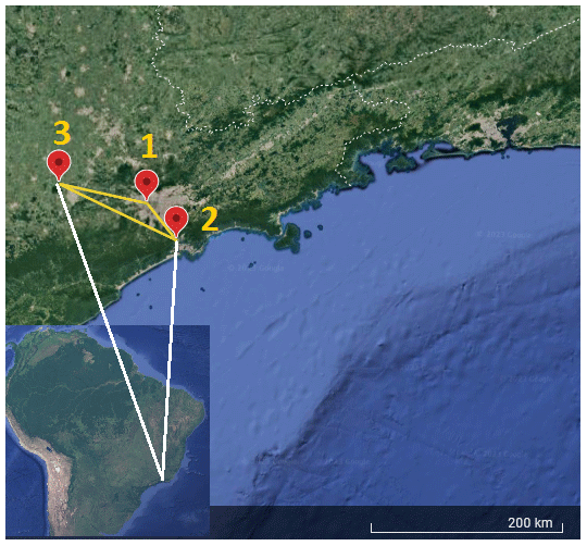
Figure 2 Sites of the observational campaigns. The distance (yellow line) is 47 km between Sites 1 and 2, 131 km between Sites 2 and 3, and 90 km between Sites 1 and 3. Distance estimated by the Google Earth tool (© Google Earth 2023).

Site 2 is a coastal municipality called Cubatão. Beyond the industrial zone, Cubatão is surrounded by natural parks of the Atlantic Rain Forest (Morellato and Haddad, 2000), residential areas and a high mountain range, called Serra do Mar, on its north boundary. At this point, Serra do Mar rises sharply, up to more than a 700 m height; is 5 km wide across; and acts as an important barrier to the atmospheric circulation. Vieira and Gramani (2015) provide a technical description of the Cubatão and Serra do Mar features.

Site 3, the Iperó municipality, is more than 130 km away from the coast, as shown in Fig. 2. It is inside a predominantly rural area and about 10 km away from the urban zone of the Sorocaba municipality. Another important characteristic of this site is the Araçoiaba hill to the southeast, rising up to more than a 300 m height up to 900 m altitude. The Araçoiaba hill is inside a Federal Conservation Unit called Ipanema National Forest.

3 Results

The surface strongly affects the atmospheric circulation within the planetary boundary layer (PBL). Thus, we plotted the wind rose for the first observational level (40 m) as an attempt to identify similarities and differences among the three sites. In this study, the wind rose shows the direction where the wind blows from (as typically used in meteorology). The circulation patterns are similar between Sites 1 and 3 (Figs. 3 and 5). Both of them present a diurnal cycle of winds turning 360°. We see this diurnal cycle in Fig. A1, which illustrates a 30 d wind direction temporal series. Most of the time, the wind turns throughout the day, except for short periods identified by the red circles, when the winds remain mainly from south–southeast and are related with postfrontal events. The sea breeze (southeast wind) is one of the main reasons for the pattern of Fig. 3 at Site 1 (Ribeiro et al., 2018). According to Ribeiro et al. (2018), there are two main conditions that inhibit the sea breeze reaching the São Paulo Metropolitan Region (SPMR): the prefrontal circulation and the cloudiness. The cloudiness decreases the thermal contrast between the sea and the land, and the prefrontal circulation is opposed to the sea breeze. Thus, excluding those two conditions, the sea breeze advances over the SPMR often throughout the year and justifies the wind rose pattern (Fig. 3). Even at 40 m above the surface, the winds are weak and rarely reach 8 m s⁻¹. However, the low-level jet (LLJ) is a typical feature of the SPMR (Sánchez et al., 2022), and the power and logarithmic law fail in extrapolating the wind speed profile in the LLJ environment when compared to machine-learning methods (Bodini and Optis, 2020a, b).

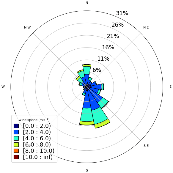
Figure 3 Observed wind at 40 m – Site 1 (normalized wind rose). The wind speed is indicated by the legend (m s⁻¹).

At Site 2 (Fig. 4), for this observational period, north and northeast winds were disproportionately more frequent than the other directions. However, it is also possible to identify a diurnal cycle, as observed in Fig. A2. Except for the postfrontal events, identified by the red circles, the wind direction is variable throughout the day. Klockow and Targa (1998) illustrated a conceptual model (their Fig. 2) and explained in a simplified way the local atmospheric circulation, where the sea and the land breezes play an important role. This frequent wind direction reversal, due to the sea–land contrast and the orography reported by Klockow and Targa (1998), may prejudice the model performance. Compared to Site 1, the wind speed is weaker. Vieira-Filho et al. (2015) also observed a similar pattern of Fig. A2 (rotating 360° throughout the day) for the surface winds and emphasized the influences of the orography and the ocean on the local circulation. They detected around 20 % of calms (wind speed < 1 m s⁻¹), occurring preferably at nighttime, and mean wind speed around 2.4 m s⁻¹.

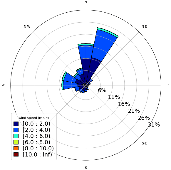
Figure 4 Observed wind at 40 m – Site 2 (normalized wind rose). The wind speed is indicated by the legend (m s⁻¹).

The diurnal cycle at Site 3 (Fig. A3) is mainly related to the mountain–valley circulation since the valley (Tietê River valley) becomes deeper towards northwest. Thus, the local circulation generally turns 360° throughout the day, resulting in the wind rose shown in Fig. 5. See that the seasonal pattern in Fig. A4 is comparable to that in Fig. 5. The circulation is also influenced by the frontal passages, and the postfrontal condition generates stronger south and southeast winds than the prefrontal condition, which generates weaker north and northwest winds. The LLJs are a recurrent feature observed at this site (de Oliveira et al., 1995) and can form very near the surface (Beu and Landulfo, 2022). Winds are slightly stronger than the other two sites but rarely reach 10 m s⁻¹ (Fig. 5).

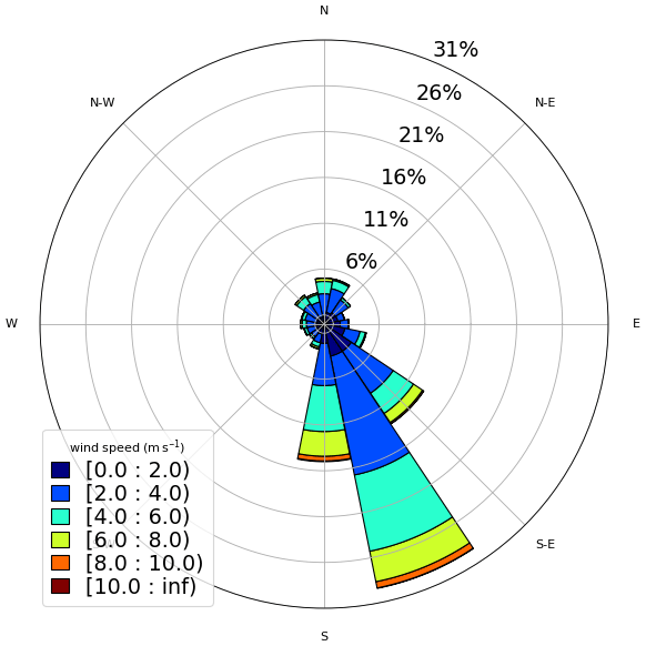
Figure 5 Observed wind at 40 m – Site 3 (normalized wind rose). The wind speed is indicated by the legend (m s⁻¹).

We carried out more than 60 experiments, testing different machine-learning models with multiple configurations, namely random forest trees (Breiman, 2001) applied by Bodini and Optis (2020a) and Bodini and Optis (2020b); SVR (Smola and Schölkopf, 2004); its two different implementations – nuSVR and LinearSVR (Pedregosa et al., 2011); multi-layer perceptron (Almeida, 1997); and complete ensemble empirical mode decomposition with adaptive noise – CEEMDAN (Torres et al., 2011). In their work, Türkan et al. (2016) used the SVR, the multi-layer perceptron and the random forest trees algorithms. CEEMDAN (Torres et al., 2011) has already been applied for wind speed forecasts (Wang et al., 2021). The LSTM RNN outperformed the SVR, nuSVR, LinearSVR, random forest trees, multi-layer perceptron and CEEMDAN. Results also improved when 10 min mean data were used as input instead of 30 min mean or 1 h mean. Here we only present results for the best-performing model LSTM RNN (Bali et al., 2019; Al-Shaikhi et al., 2022).

3.1 Experiment 1

Data from Site 3 was first used to train the model, starting with wind speeds at 40 m to predict speeds at higher heights. The entire dataset contains more than 50 000 data points for each variable. As we were working at Colab, for each new test it was necessary to upload the dataset. Inputting the whole dataset for training and testing the model consumes much processing time. Considering we were working at Google Colab, for each new test it was necessary to upload the dataset again. Despite this, running machine learning on Colab is advantageous, in the sense that many libraries are easily accessible and do not require installation at the local machine. The Google Colab also eases the team work, since the code can be safely shared with the group members. Surprisingly, we found that model improvement plateaued without using all of the data points of record. During this phase we conducted tests changing the dataset size and hyperparameters and evaluated the improvement through the metrics (Eqs. 10 to 14).

For Site 3, we found that the ideal dataset size was 8 000 data points, taking 90 % for the training. As the time series is comprised of 10 min temporal averages, that corresponds to roughly 2 months of observational data. We proceeded to test the inclusion of other variables, such as wind direction, hour and TKE (Eq. 8), because those data give information about the diurnal cycle and improve the model. Tables 2–4 and Figs. 6–8 present the results reached by the LSTM model and the power law (PL), according to Eq. (9) and α=0.25, as we found that this value provides the best correlation for our datasets. See Table A1 for the dataset sizes and hyperparameters. For all three sites, the R² is similar for estimates with the PL and the LSTM at the first level (60 m); however, as the distance from the surface increases, the LSTM estimates outperform the PL. That behavior was also observed by Liu et al. (2023). This happens because the PL has a universal nature and cannot simulate features like the LLJ (Bodini and Optis, 2020a).

Table 2 Site 1 – assessment of the wind speed estimated by the PL and the LSTM model (Experiment 1) up to 230 m.

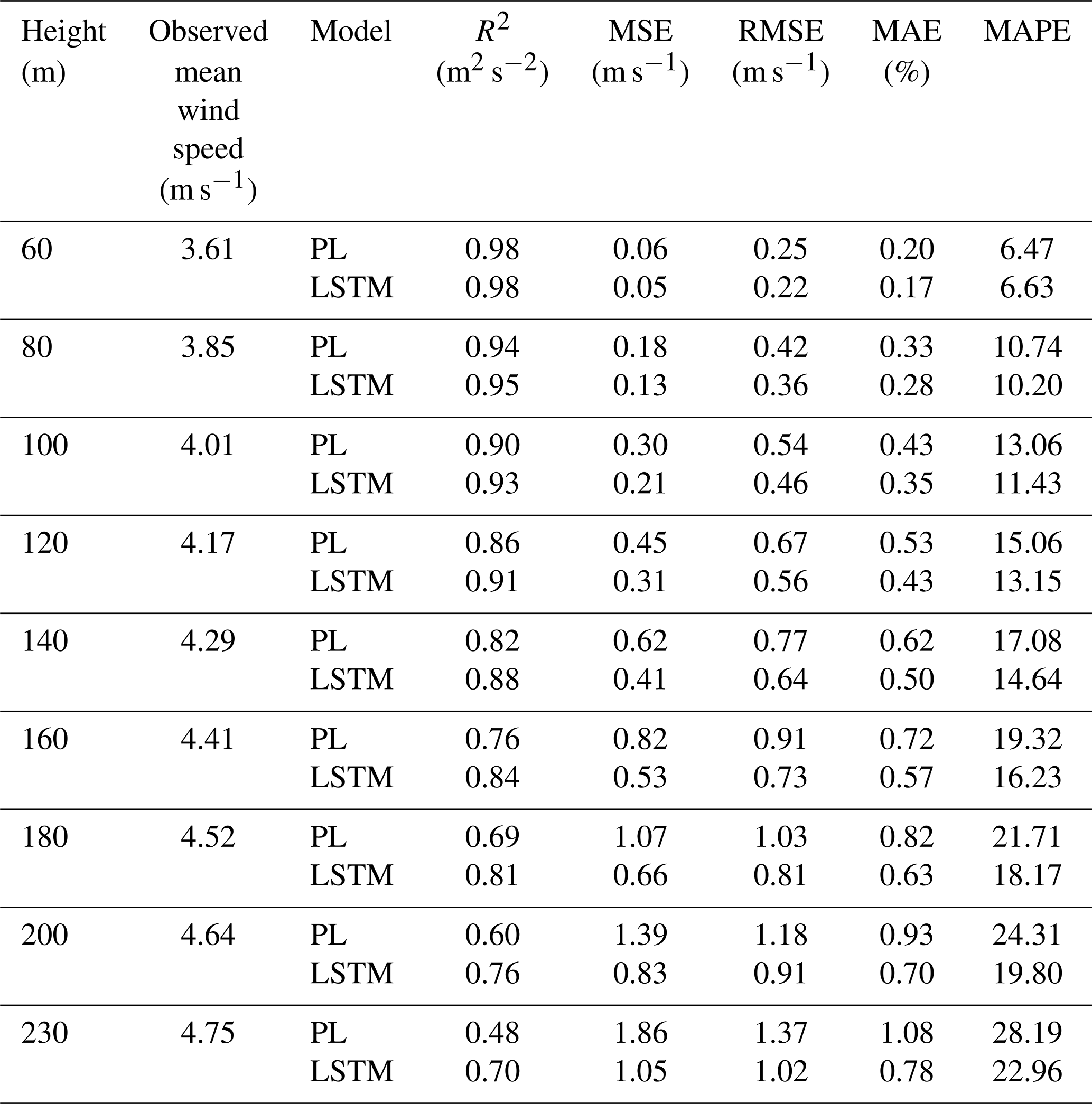
Table 3 Site 2 – assessment of the wind speed estimated by the PL and the LSTM model (Experiment 1) up to 230 m.

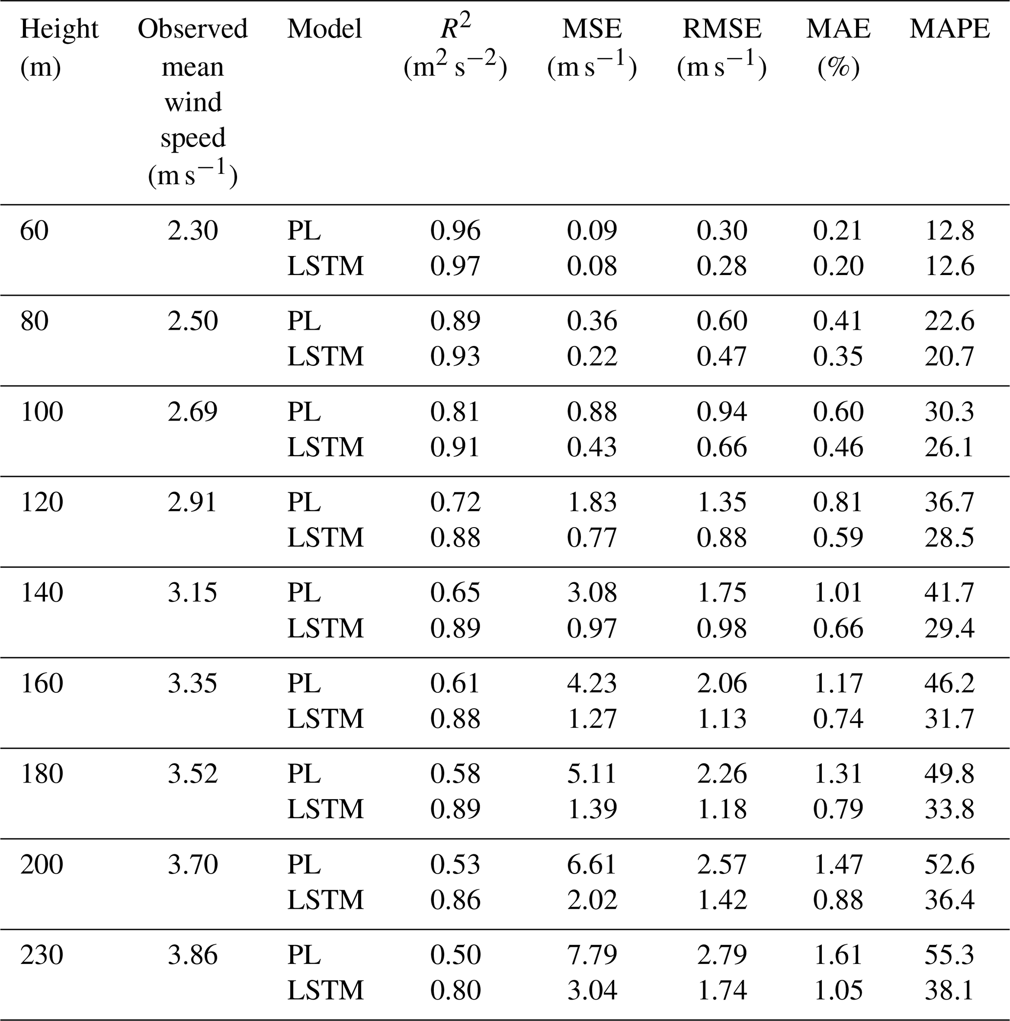
Table 4 Site 3 – assessment of the wind speed estimated by the PL and the LSTM model (Experiment 1) up to 230 m.

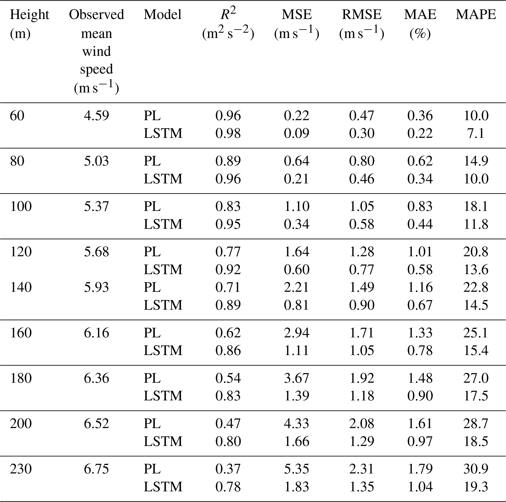
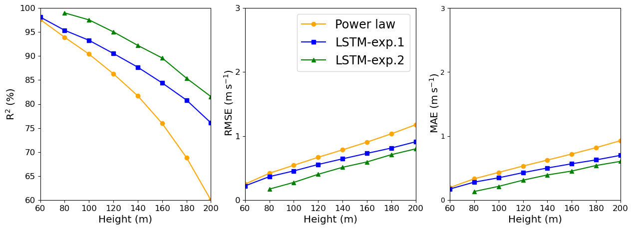
Figure 6 LSTM and power law R², RMSE, and MAE estimates: Site 1. In the legend, exp.1 and exp.2 stand for Experiment 1 and Experiment 2, respectively.

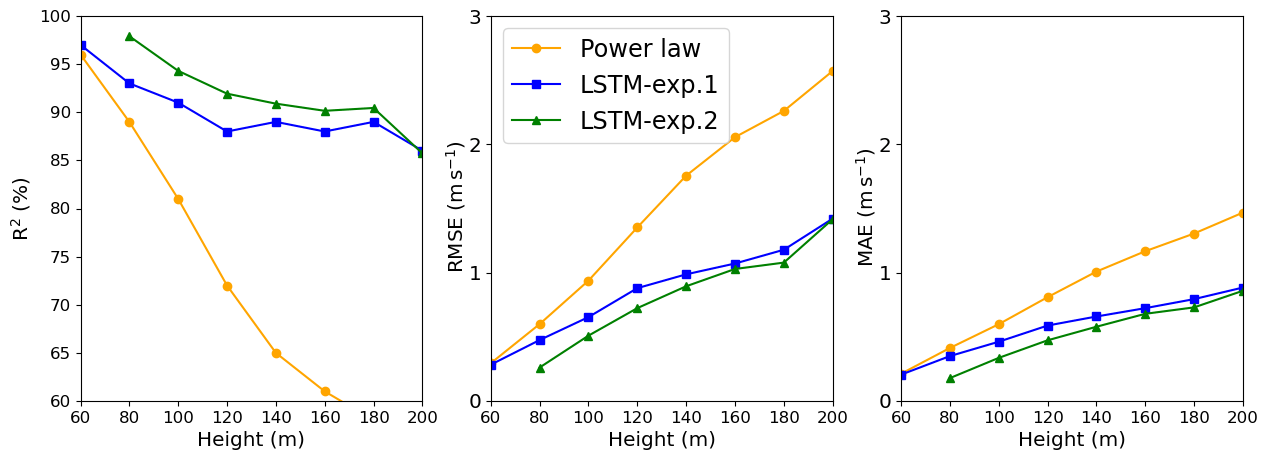
Figure 7 LSTM and power law R², RMSE, and MAE estimates: Site 2. In the legend, exp.1 and exp.2 stand for Experiment 1 and Experiment 2, respectively.

Figure 8 LSTM and power law R², RMSE, and MAE estimates: Site 3. In the legend, exp.1 and exp.2 stand for Experiment 1 and Experiment 2, respectively.

For Site 1, we reached the best result with a temporal series with 10 000 data points. This is approximately a 70 d observational campaign. When only 40 m variables are used as predictors, we obtain R²>90 % up to 120 m (Table 2). The MSE and MAE also confirm the superiority of the LSTM model over the PL. Even the MAPE is greater for the PL estimates than for the LSTM estimates.

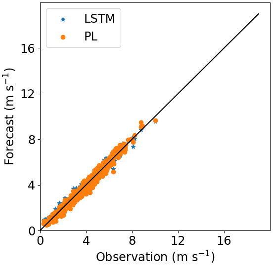
Comparing Site 1 and Site 3, we see through Figs. 6 and 8 that the PL performance decreases faster at Site 3 than at Site 1. At 160 m, the R²=62 % at Site 3 and R²=76 % at Site 1. For Site 2, the PL performance also exhibits a rapid decrease with the height (Fig. 7), similarly to Site 3. Summarizing, we see from Figs. 6–8 that the PL works better close to the surface. Looking at the scatter plot for Site 1, we see that the PL performance compares to the LSTM (Fig. 9) at 60 m, but at 230 m we see stronger winds underestimated by the PL (the red circle on Fig. 10).

Figure 9 LSTM and PL forecasts (Site 3) for 60 m – results from Experiment 1.

Figure 10 LSTM and PL forecasts (Site 3) for 230 m – results from Experiment 1.

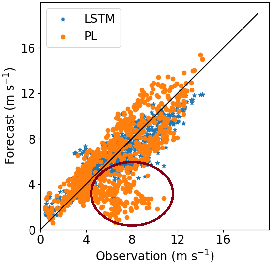
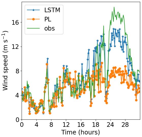
Site 2, which has weaker winds (see Table 3, column 2), presents better performance for the LSTM forecast from 140 m upwards than the other two sites. As shown by Fig. 7, R² remains almost constant above 140 m, while for the PL, the R² decreases faster than the Site 1 curve. The PL underestimates winds stronger than 8 m s⁻¹ as illustrated by the scatter plot (Fig. 11) and are associated with abrupt changes as indicated by the temporal series (Fig. 12). The causes of that strengthening of the wind profile are unknown and remain as suggestion for a future investigation. The LSTM also underestimates the stronger winds (mainly the winds that exceed 12 m s⁻¹), as we see from the scatter plot, but it captures the pattern better than the PL (Fig. 12).

Figure 11 Site 2: 160 m wind speed forecast (Experiment 1).

Figure 12 Site 2: 160 m wind speed temporal series (Experiment 1).

The metrics show a similar behavior between Site 1 and Site 3. Despite the complex topography, perhaps the better performance of the LSTM model for Site 2 for the levels above 140 m is related to the absence of the LLJ. To the best of our knowledge, LLJs so close to the surface have not been reported there yet; on the contrary, they are a common feature of Sites 1 and 3 (Sánchez et al., 2022; de Oliveira et al., 1995; Beu and Landulfo, 2022).

3.2 Experiment 2

Some studies (e.g., Vassallo et al., 2020; Mohandes and Rehman, 2018) already showed that adding input variables from different heights below the extrapolation height improves the machine-learning performances. Thus, we added the 60 m wind speed observations to the input dataset of Experiment 1 to estimate the above heights. Adding the 60 m wind speed observations to the input dataset improved the results, as we see in Figs. 6,–8 (green line). For Site 1 we see an increasing along the entire R² curve, reaching 99 % at 80 m, while the MAE decreased by 50 %. At 200 m, the R² increased by 6 % and the MAE decreased by more than 8 %. The improvement was more pronounced at the lower heights for Site 2 (compare the blue and green lines in Fig. 7). The R² increased to 98 % against the 93 % from Experiment 1 at 80 m, and the MAPE was reduced by 70 %, but for the higher levels, the improvement gradually decreases, as we see from Fig. 7.

For Site 3, Experiment 2 also outperformed Experiment 1, and the improvement is constant with the height, just slightly better at 80 m as we see from the greater distance between the green and blue lines (Fig. 8). The R² increased 2.5 % at 80 m and only 1.5 % at 200 m. Performing the bootstrapping method (Figs. A5–A7), it is evident that the variability is higher for the PL estimate for Sites 2 and 3, mainly. For Site 1, despite the LSTM-exp.2 exhibiting similar error bars, the R² is higher.

We also found that the performance is kept if we change the sample size for the tests. For the tests, we evaluated the R² for three different samples beyond those from Table A1. Tests were done for 2000, 4000 and 7000 data points. For the PL estimate, the α was computed taking the 40 and 60 m wind speed. The results for the 80 and 180 m forecasts are shown in Fig. A8. We see that the R² values are comparable for the LSTM and PL estimates and remain almost constant for the 80 m forecast for the tests conducted with 2000, 4000 and 7000 data points at Site 1. For the 180 m forecast, the LSTM performance slightly increases when the sample dataset increases from 2000 to 7000. For the Site 3 case, the 80 m forecast presented only slight variation, and LSTM and PL performances are also comparable. Site 2 forecasts exhibited a slight improvement when the test dataset increased from 2000 to 7000 data points at 80 m. In this case, the PL performance was worse than the LSTM. The 180 m forecast for Site 2 is not shown because the original dataset reported an atypical pattern, with the 180 m wind speed weaker than the 40 m wind speed. Because of that atypical pattern, even the PL estimate failed. The PL estimates at 180 m for Sites 1 and 2 were also worse than the LSTM forecast and are not shown because they are out of the figure scale.

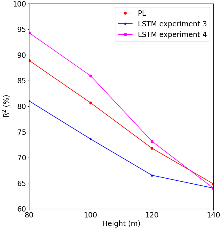
3.3 Experiment 3

Bodini and Optis (2020b) advised about the importance of applying the machine-learning models to different sites than where they were trained. Following their advice, we applied each trained model to the other two sites (Figs. 13–15).

Figure 13 Comparison between Experiment 1 and Experiment 3, where S1 is the result of Experiment 1, S1(S2) is the forecast for Site 1 run with the model of Site 2, and S1(S3) is the forecast for Site 1 run with the model of Site 3.

Figure 14 Comparison between Experiment 1 and Experiment 3, where S2 is the result of Experiment 1, S2(S1) is the forecast for Site 2 run with the model of Site 1, and S2(S3) is the forecast for Site 2 run with the model of Site 3.

Figure 15 Comparison between Experiment 1 and Experiment 3, where S3 is the result of Experiment 1, S3(S1) is the forecast for Site 3 run with the model of Site 1, and S3(S2) is the forecast for Site 3 run with the model of Site 1.

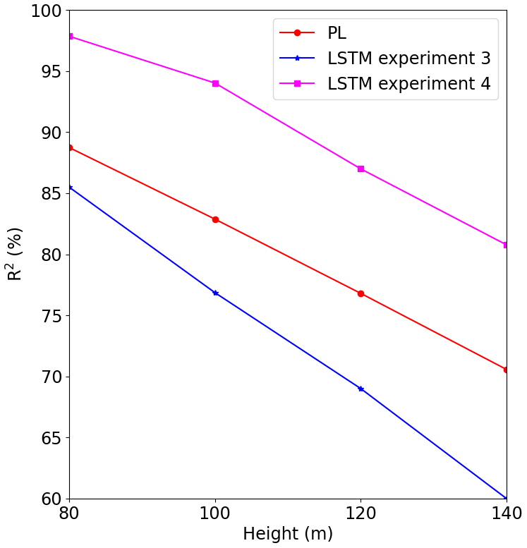
For Site 1 (Fig. 13) we see that the Site 3 model (blue line) performed better than the Site 2 model (green line), but its performance was worse than the original model (S1, which was trained and validated at Site 1). It is also clear from this figure that the performance quickly decreases with the height. The behavior is the same for Site 3 (Fig. 15), where the model trained for Site 2 presented the worst result. The tests of the models trained at Site 1 and Site 3 for Site 2 presented poor performance as indicated by the fast R² reduction with the height (Fig. 14).

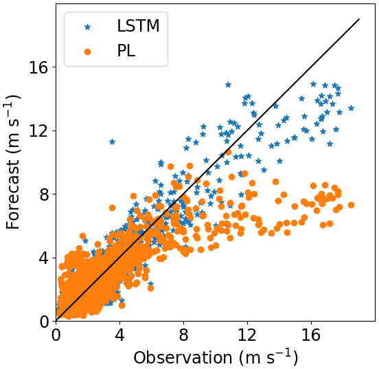
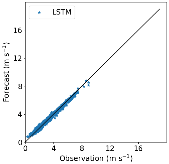
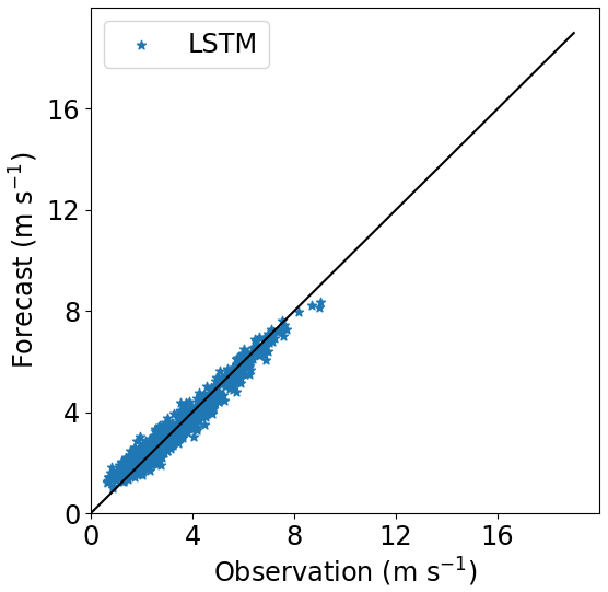
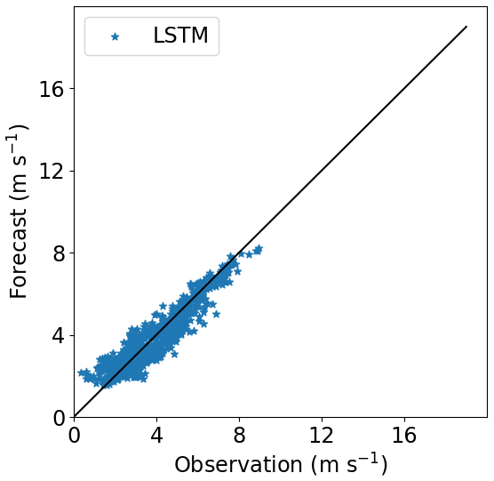
Figures 16–18 show the correlation between observed and forecasted wind speed for 80, 100 and 140 m for the forecast of Site 1 with the model trained at Site 3.

Figure 16 Correlation between forecasted and observed data for Site 1 with the model trained at Site 3. Height: 80 m.

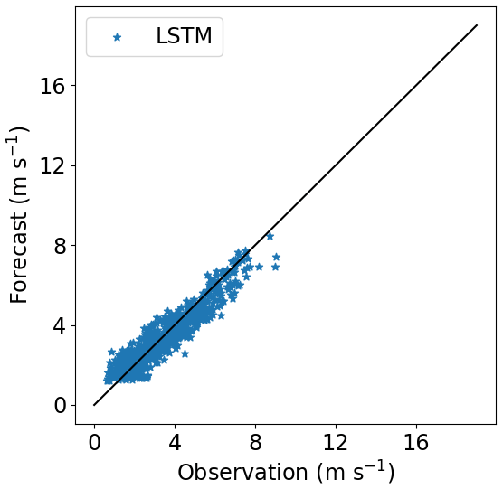
Figure 17 Correlation between forecasted and observed data for Site 1 with the model trained at Site 3. Height: 100 m.

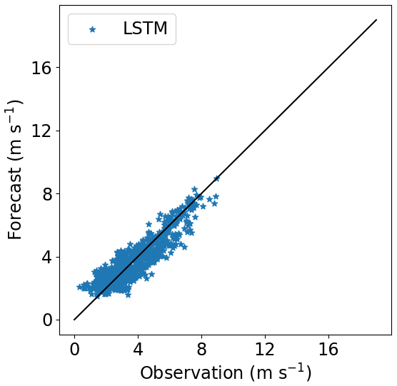
Figure 18 Correlation between forecasted and observed data for Site 1 with the model trained at Site 3. Height: 140 m.

3.4 Experiment 4

For this step, we took the best result from the previous experiment (Experiment 3) and added the 60 m wind speed to the input dataset. That means, for the Site 1 case, we took the model trained at Site 3.

The forecast for Site 1 highly improves when the 60 m wind speed is included on the input dataset for training the model at Site 3, as we see in Fig. 19, and it outperforms the PL forecast. The R² increased by 7 % if compared with the LSTM forecast with only the 40 m observations (Experiment 3) for the 80 m height. The R² reached 90.6 % and 84.9 % at 120 and 140 m, respectively. This result is almost as good as Experiment 1. Figures 22–24 illustrate the improvement (compared to Figs. 16–18) when the 60 m wind speed observation was added to the training phase.

Figure 19 Site 1: comparison for the PL, Experiment 3 and Experiment 4 estimates.

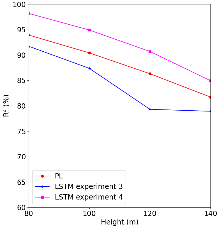
We also observe a strong improvement for Site 3 (Fig. 21) compared to the PL estimate. At 80 m, the R² increased by 9 % compared to the PL estimate, while at 140 m, we observed an increase of 16 %.

For Site 2 we used the model trained at Site 1, since that one performed best, as indicated by Fig. 14. In this case, we see improvement up to 120 m (Fig. 20), but it was less than the other two cases. It is obvious that adding more observational levels to the input dataset would improve the results; however, it is not clear if this method should be applied if the surfaces are too different as Site 2 is in relation to Site 1 and Site 3. We recommend more tests for the complex terrain scenarios.

Figure 20 Site 2: comparison for the PL, Experiment 3 and Experiment 4 estimates.

Figure 21 Site 3: comparison for the PL, Experiment 3 and Experiment 4 estimates.

Figure 22 As Fig. 16, except the 60 m wind speed was added to the input dataset.

Figure 23 As Fig. 17, except the 60 m wind speed was added to the input dataset.

Figure 24 As Fig. 18, except the 60 m wind speed was added to the input dataset.

4 Conclusions

Nowadays, the machine-learning techniques produce successful results to forecast environmental processes. However, forecasting the wind speed is still a challenge due its random nature, and researchers are dedicating considerable time and efforts to reach confident results. Comparative studies showed the superiority of the LSTM to forecast the wind speed against other machine-learning techniques. Adding more meteorological variables has also improved the results. Ensemble and hybrid methods are strategies that also contribute to the model performances.

Only recently have machine-learning techniques been applied to extrapolate the wind speed to higher heights. The models generally require large datasets with some observational heights. After testing some commonly used algorithms for the wind speed forecast (random forest trees, support vector regression and multi-layer perceptron), we found the LSTM outperformed all of them. The LSTM outperformed even the decomposition methods.

We also evaluated different dataset sizes and found that the model did not improve even if the dataset size increases beyond that presented in Table A1; however, the model is sensitive to the training data percentage. In this study, taking 90 % of the dataset for training produced the best result. The tests also showed best results for 10 min mean as input data compared to 30 min or 1 h mean.

Including the 40 m wind direction, TKE and the hour in the input dataset improved the model, which outperformed the power law as the distance from the surface increases. Adding the 60 m wind speed observations to the dataset improved the results, as expected from results of previous studies. However, the improvement was better for Sites 1 and 2 than for Site 3. The causes should be investigated in future work.

Even over complex terrain and with a relatively short dataset (an observational campaign shorter than 3 months), the LSTM outperformed the power law. The power law cannot reproduce features like the LLJs that are often observed, at least over Sites 1 and 3. Site 2 is strongly influenced by the sea and land breezes, and the LSTM model captured the abrupt changes of the wind profile better than the power law.

The results found in this observational campaign, albeit short, show the benefits of Doppler lidars in improving model results to estimate winds at height. This is particularly relevant to help support the energy transition and net zero targets. Despite the costs associated with Doppler lidars, the authors would encourage further strategic collaborations to drive observational data improvements leading to advances in model prediction.

As future work, we intend to follow two different approaches. As we got better results with 10 min mean than with 1 h mean observational data, we want to test the LSTM recurrent neural network providing a higher-temporal-resolution dataset, like 1 or 5 min means, instead of 10 min means, as provided for this study. Even if this requires a new observational campaign, we could evaluate the benefits of increasing the temporal resolution of the dataset. As a second approach we would like to evaluate the benefits of adding other sources, like reanalysis data or more observational data, such as surface pressure, surface temperature, and 2 and 10 m wind data. Concerning machine-learning techniques, we suggest a deeper investigation through hybrid and ensemble methods.

Appendix A

Table A1 Dataset size and hyperparameters.

Table A2 LSTM arguments.

Table A3 Data availability (%).

Table A4 Input variables.

Figure A1 Site 1: wind direction temporal series.

Figure A2 Site 2: wind direction temporal series.

Figure A3 Site 3: wind direction temporal series.

Figure A4 Site 3: observed wind at 40 m (normalized).

Figure A5 Site 1: R² error bars.

Figure A6 Site 2: R² error bars.

Figure A7 Site 3: R² error bars.

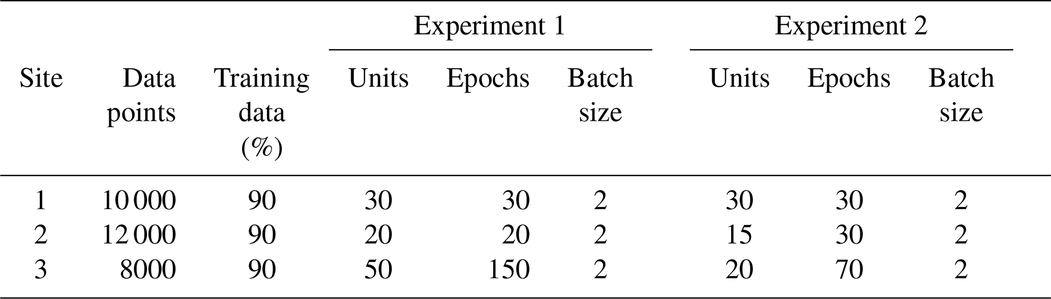
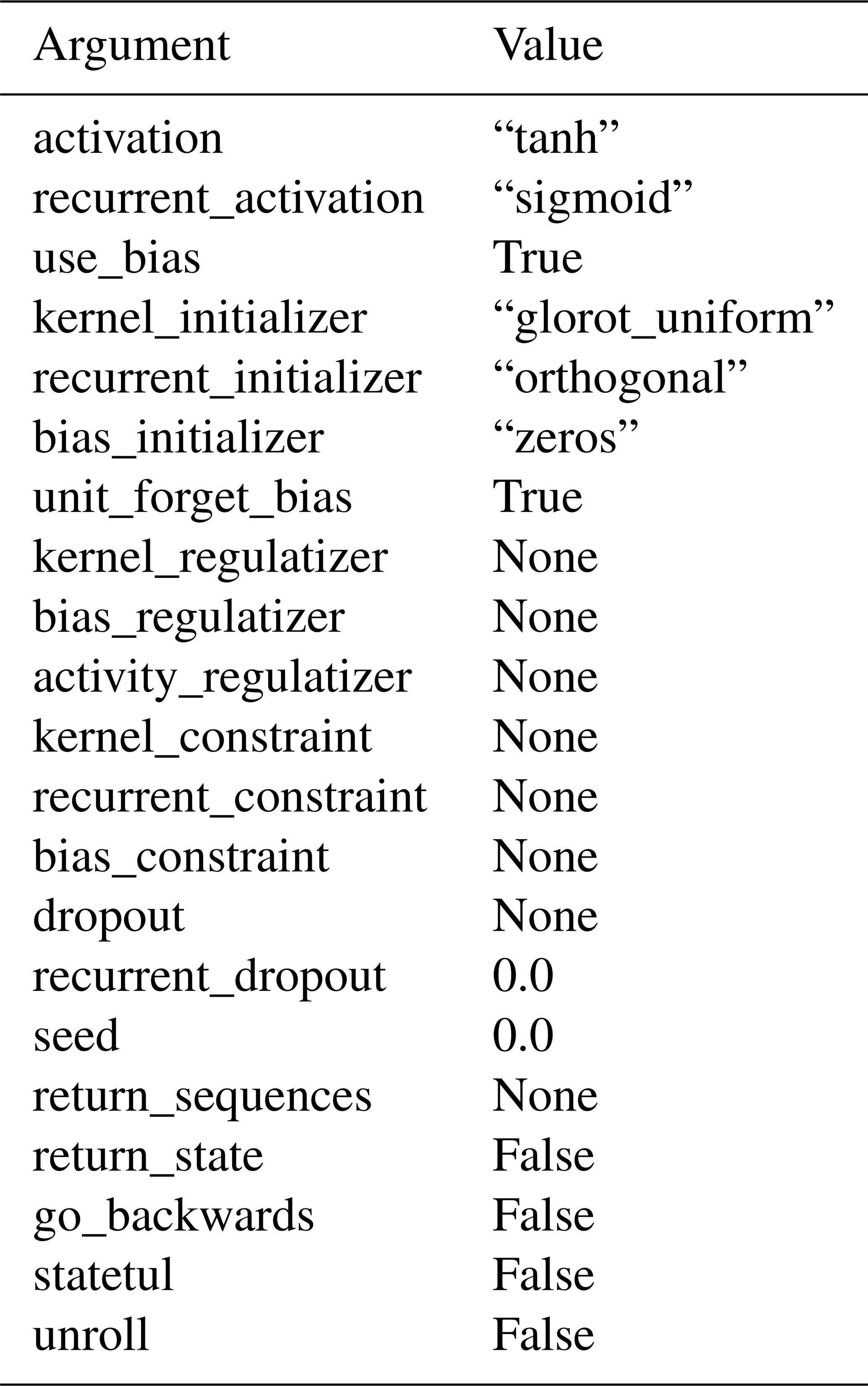
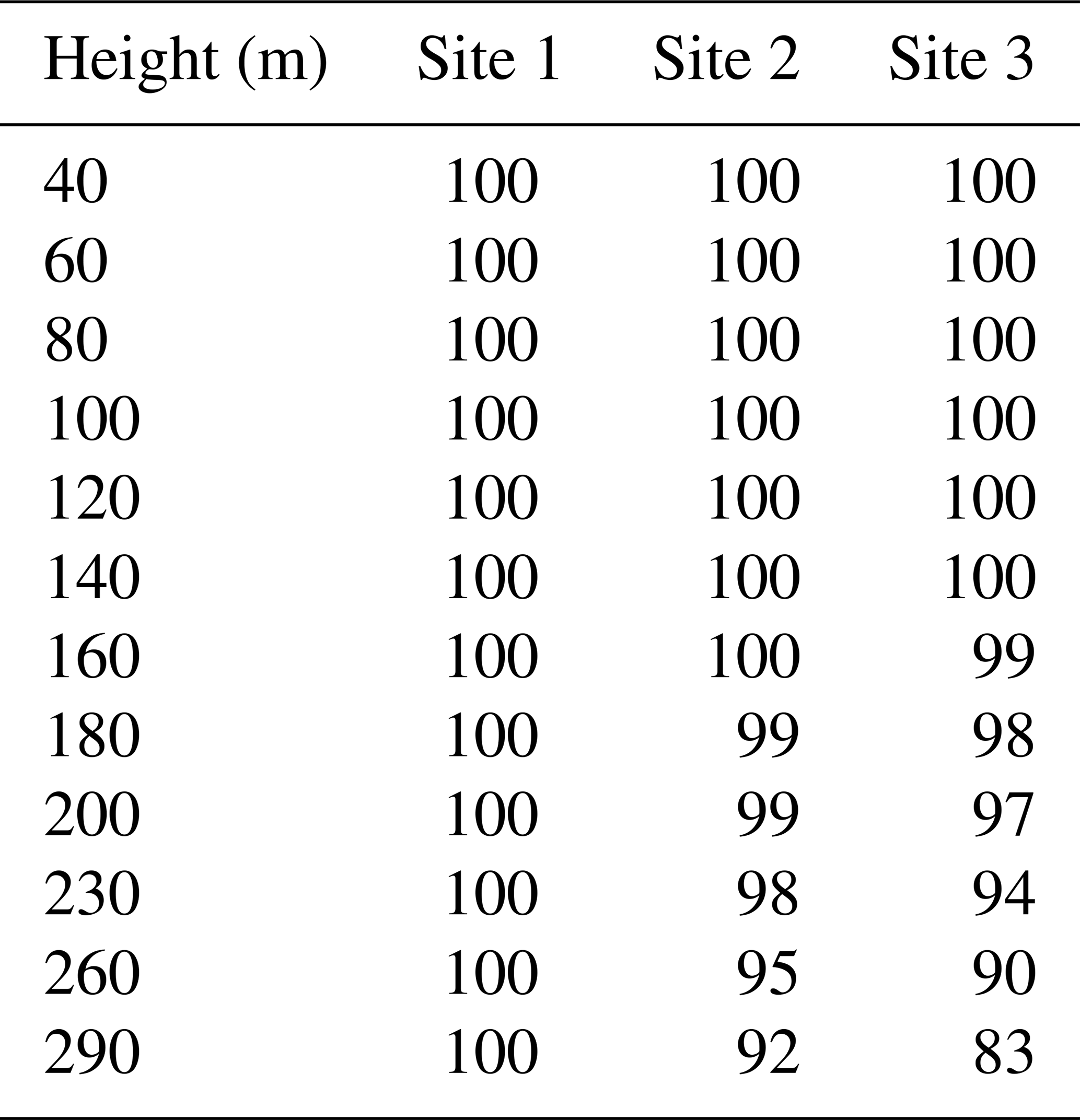
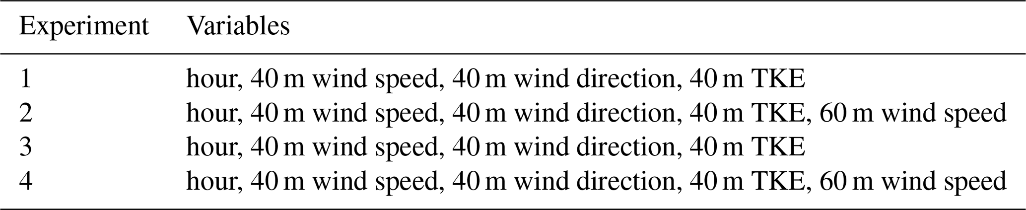
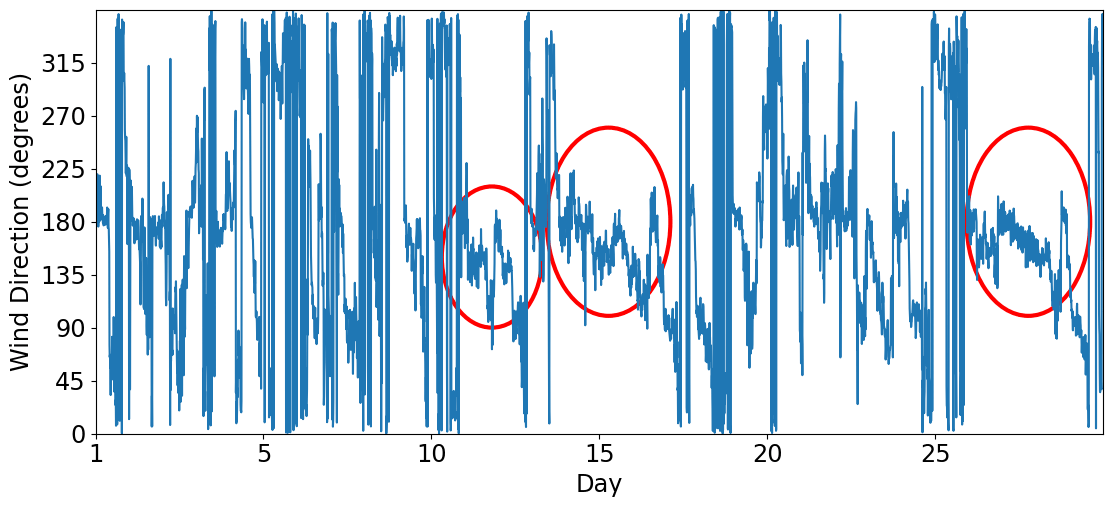
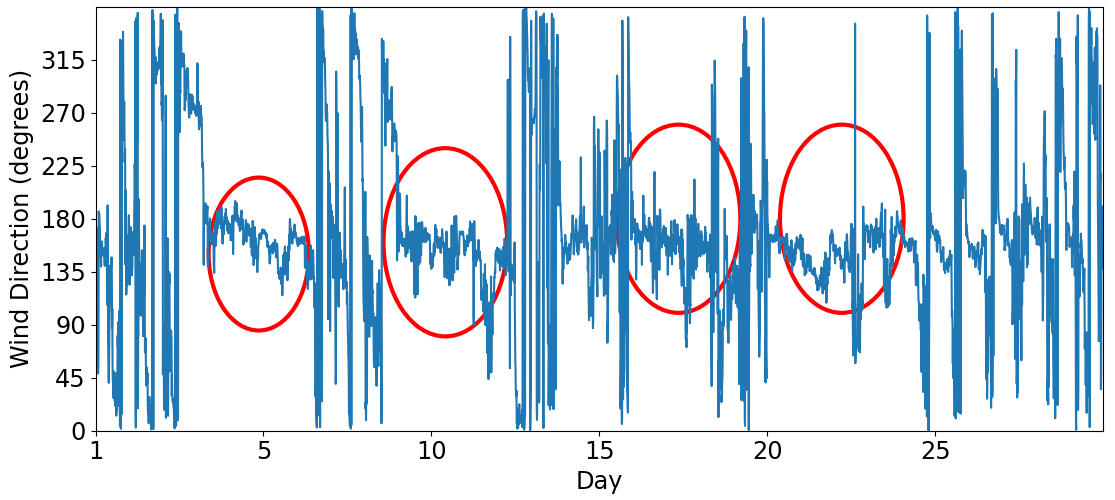
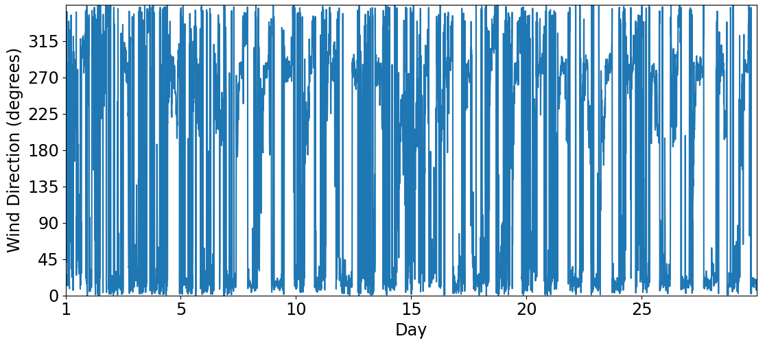
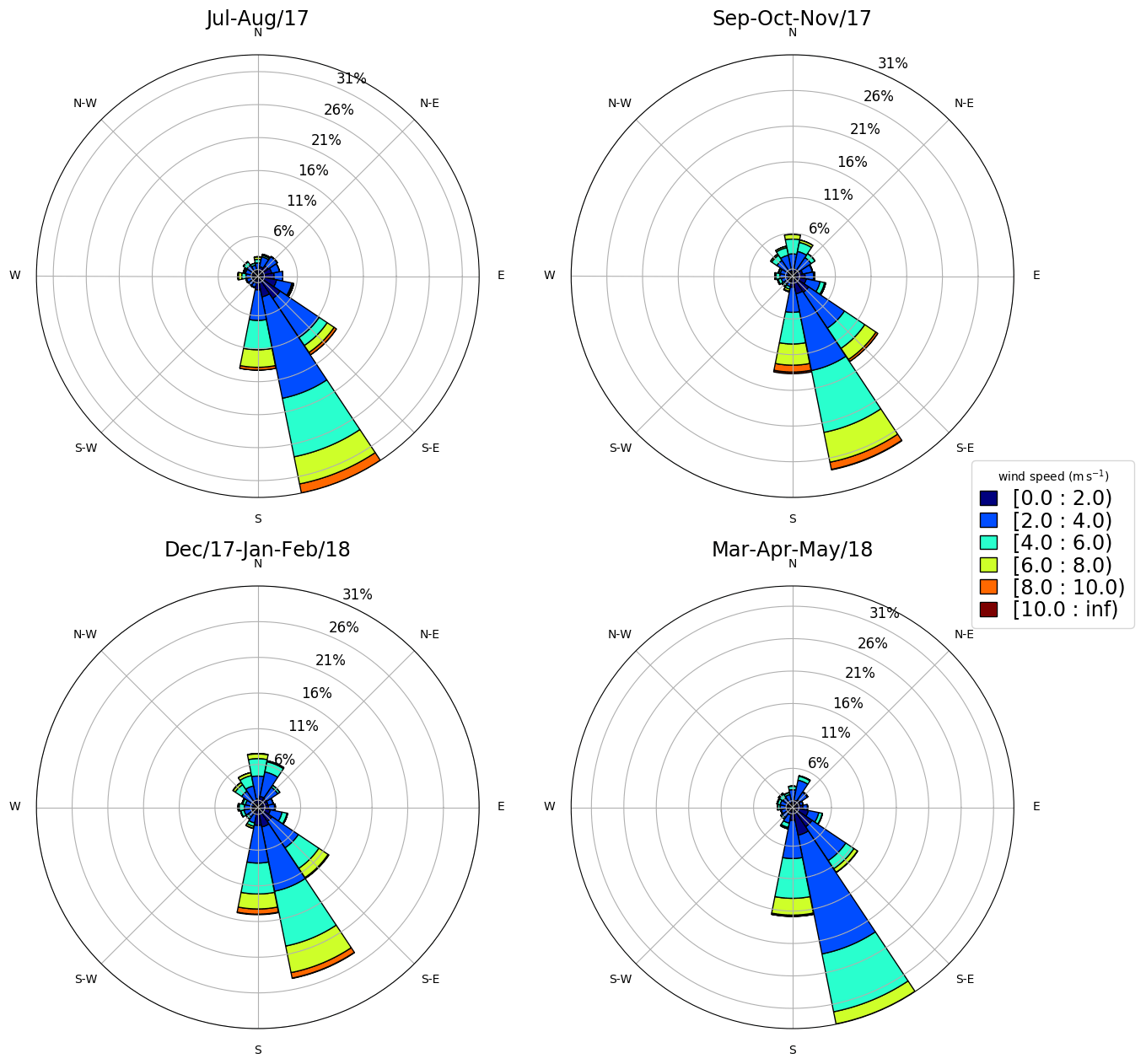
Figure A8 R² versus sample size of the Experiment 2 tests. α estimated from observational 40 and 60 m wind speed.