the Creative Commons Attribution 4.0 License.
the Creative Commons Attribution 4.0 License.
 | 08 Jul 2024
Comparison of different cross-sectional approaches for the structural design and optimization of composite wind turbine blades based on beam models
Daniel Hardt
Claudio Balzani
Christian Hühne
During the preliminary design phase of wind turbine blades, the evaluation of many design candidates in a short period of time plays an important role. Computationally efficient methods for the structural analysis that correctly predict stiffness matrix entries for beam models including the (bend–twist) coupling terms are thus needed. The present paper provides an extended overview of available approaches and shows their abilities to fulfill the requirements for the composite design of rotor blades with respect to accuracy and computational efficiency. Three cross-sectional theories are selected and implemented to compare the prediction quality of the cross-sectional coupling stiffness terms and the stress distribution based on different multi-cell test cross-sections. The cross-sectional results are compared with the 2D finite element code BECAS and are discussed in the context of accuracy and computational efficiency. The analytical solution performing best shows very small deviations in the stiffness matrix entries compared to BECAS (below 1 % in the majority of test cases). It achieved a better resolution of the stress distribution and a computation time that is more than an order of magnitude smaller using the same spatial discretization. The deviations of the stress distributions are below 10 % for most test cases. The analytical solution can thus be rated as a feasible approach for a beam-based pre-design of wind turbine rotor blades.
- Article
(3378 KB) - Full-text XML
- BibTeX
- EndNote


Beam-based approaches are commonly used in the conceptual and preliminary structural design of wind turbine blades. They are often embedded in a multi-disciplinary optimization (MDO) process (Scott et al., 2019; Serafeim et al., 2022) due to a superior computational performance compared to high-fidelity finite element (FE) models using shell and/or solid elements. A typical application of MDO is the design of rotor blades with tailored bend–twist coupling (Scott et al., 2020; Bottasso et al., 2012). The blade flexibility affects the angle of attack along the blade and thereby changes the lift and drag force distribution, reducing the flapwise bending moments. For the structural optimization in general, a common objective function is the reduction of mass or costs (Lee and Shin, 2022).
For larger blades, mass and costs increase to the power of around 2.4 with the blade radius (Rosemeier and Krimmer, 2022), whereas the annual energy production (AEP) increases proportionally to the square of the blade radius (Gasch and Twele, 2012). Hence, the blade mass and costs scale over-proportionally compared with the AEP. It is thus required to investigate new technologies, materials, or designs to withstand the increased mass-related loads and to limit the blade costs, which are a significant part of the overall turbine costs.
1.1 Beam models within the design process of wind turbine blades
The usage of beam models becomes necessary within the structural optimization in the preliminary design phase due to the evaluation of many design candidates. The number of design candidates results from the investigation of different designs for the structural topology (e.g., number and/or positions of spars) and concepts for materials used and how they are combined in laminate layups, which in turn have to be linked to a manufacturing concept. Consequently, a basic requirement is a significant reduction of the computation time for model creation and the calculation of stresses compared to a high-fidelity FE model. The computation time for the stress calculation scales with the number of iterations of the optimization process. For the shell or solid FE model case, variations of the internal structure of the blade, e.g., the spar position, often require a 3D CAD (computer aided design) model update and the subsequent translation into a new FE mesh. The higher modeling effort and the longer computation times with 3D models are not acceptable in the preliminary design phase.
FE beam models require the input of accurate cross-sectional properties, i.e., stiffness and mass matrices. In many design processes (e.g., Scott et al., 2019; Wanke et al., 2021), the cross-sectional properties are determined using 2D FE models that serve to calculate the mass and stiffness properties and the stress distribution within the cross-section. These 2D FE approaches suffer from the need of expensive model updating, with re-meshing if the internal structure or layup changes during the optimization process, and from higher computation costs for solving the governing equations compared to analytical approaches.
1.2 Requirements for an analytical cross-sectional approach
Requirements for an analytical cross-sectional calculation module are derived in the following and serve to evaluate different calculation methods at a later stage. Composite blades are modeled as beams with closed, different single- or multi-cell cross-sections that vary along the beam axis. The parts of the blade, e.g., shell panels and spars, consist of different materials. Moreover, different materials within one part can occur. The structure of the blade is mostly thin-walled, except near the blade root, and undergoes in-plane and out-of-plane cross-sectional deformations. Beside the classical loading of thin-walled beams such as bending or extension, shear forces play an important role and can be design drivers. The couplings of the beam's degrees of freedom that result from the structural topology or the material layup have to be considered for an accurate representation of the blade. The computational efficiency, i.e., fast output with high accuracy, is of high importance as well to allow the assessment of a large number of design candidates in the preliminary design phase.
The historical development of cross-sectional approaches for general beam structures is described by Hodges (2006). Chen et al. (2010) compare several existing tools for cross-sectional calculations, e.g., PreComp (Bir, 2006) or VABS (Yu, 2007).
1.3 Target setting
The present paper provides a comprehensive review of available cross-sectional approaches (Sect. 2.4) based on the aforementioned requirements for the design of composite wind turbine rotor blades. Three cross-sectional theories are selected (Sect. 2.5) and implemented. The results of the different methods, i.e., the cross-sectional coupling stiffness terms (e.g., extension–torsion, bending–torsion, Sect. 3.2) and the stress distributions in different cross-sections (Sect. 3.3), are compared. A rectangular and a multi-cell airfoil-based cross-section serve as test cases. The focus is on the shear stress distribution caused by transverse shear forces, as these are more complex to calculate compared to, e.g., bending-related normal stresses. The cross-sectional results are verified using the 2D FE code BECAS (Blasques, 2012), which is a well-established industry standard in rotor blade design and serves as a reference solution in this paper. A verification of BECAS itself using VABS, which is also a 2D FE code for the calculation of beam cross-sectional properties (Yu, 2007), is given in Blasques (2012). The three selected analytical approaches are evaluated with respect to accuracy of the cross-sectional results and the computation time. The best compromise serves as basis for the cross-sectional calculation module of the beam-based design tool PreDoCS (Preliminary Design of Composite Structures).
A beam is a mechanical model of a structure that is characterized by a configuration where one geometric dimension is at least 1 order of magnitude larger than the other two. This allows the beam to be represented by two-dimensional cross-sections (formed by the shorter geometric dimensions) threaded along the beam axis (the longer geometric dimension). The calculation of the beam is thus subdivided into the 2D calculation of cross-sectional properties and a line-like calculation of the beam (often referred to as 1D analysis), with its axis being potentially curvilinear in space. This procedure is also called dimensional reduction (Hodges, 2006) and is described in the following subsections.
2.1 Recovery relations between beam and cross-section
The first step is to set up the kinematic relations that link the displacements in each point of a cross-section to the displacements and rotations, or curvatures, of the beam at the respective axial position. These relations are also called “recovery relations”. The formulation of the cross-sectional displacements is the core of the cross-sectional theory. From these, the cross-sectional strains are calculated as the derivatives of the displacements. In a second step, the constitutive relations of the material (material stiffness) are used to calculate the stress distribution in the cross-section from the strains. The cross-sectional stiffness matrix is derived using the principle of virtual work. The spatial integration of the stress and strain distributions across the cross-section yields the internal loads (cutting forces and moments) acting on the respective cross-section. Substituting the stresses and strains by the kinematic and the constitutive equations of the material results in the relation between the displacements and the internal loads of the cross-section which forms the cross-sectional stiffness matrix.
2.2 Finite beam element model
In the case of simple load cases (defined by loads and boundary conditions) and beams with a constant cross-section, the displacements along the beam can be calculated analytically. For more complex load cases and geometries, a finite beam element model using the cross-sectional stiffness matrices from above needs to be employed. Solving the finite element problem yields the displacements and rotations along the beam. The recovery relations from the previous subsection can then be used to calculate the cross-sectional displacements at each point along the beam. The strain and stress distributions are subsequently calculated according to the cross-sectional theory as described in the previous subsection (Hodges, 2006).
2.3 Degrees of freedom of a cross-section
In general, the cross-sectional stiffness relations of a beam are given by the expression
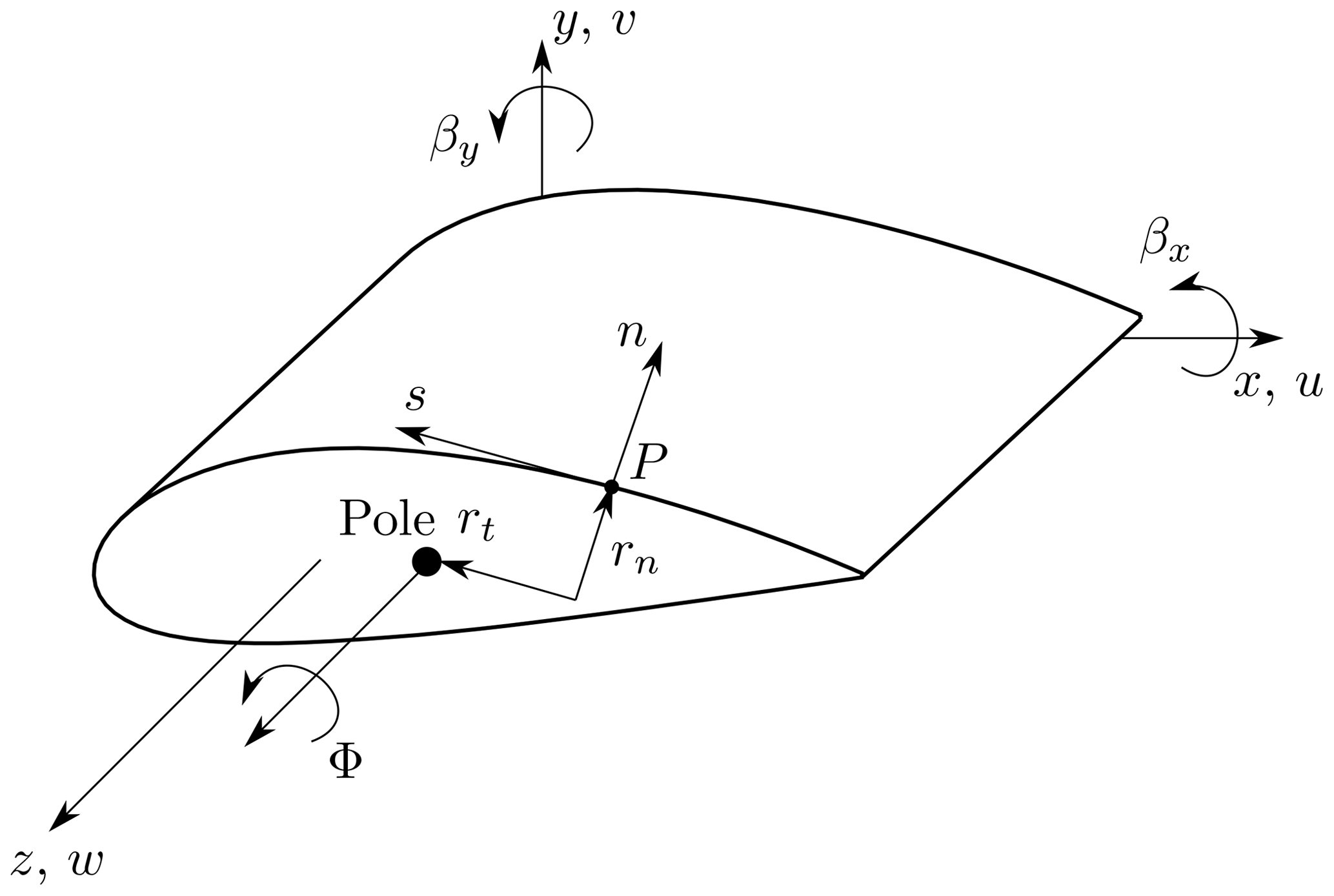
where K is the cross-sectional stiffness matrix, q is the vector of cross-sectional displacements, and F is the vector of the cross-sectional internal loads according to the notation of Jung and Nagaraj (2002). For simplicity, a notation of partial derivatives with subscripts is used, i.e., . As described by Hodges (2006), the cross-sectional degrees of freedom (DOFs) depend on the theory. Thus, the dimensions of q, F, and K also depend on the theory used. The local coordinate system and the DOFs are shown in Fig. 1. The longitudinal direction of the beam is denoted by the z axis, and the cross-sectional plane is spanned by the x and y axes, respectively.
If only DOFs for bending and extension are considered, the Euler–Bernoulli beam theory is employed. It has three cross-sectional DOFs, which are namely the longitudinal strain w0,z and the derivative of the rotation about the two axes parallel to the cross-sectional plane, βx,z and βy,z. Hence, q has three entries, and K is of order 3×3. In order to consider shear deformation, the Timoshenko beam theory can be used, which is also referred to as the first-order shear deformation theory (FSDT). The cross-section has two additional DOFs in this case, which are the shear deformation angle in the x–z plane γxz and the shear deformation angle in the y–z plane γyz. The vector of cross-sectional displacements q is then extended to five entries, and K is of order 5×5. In addition, the extension, bending, and shear parts can be supplemented by a contribution from torsion by including the respective DOFs. The St. Venant theory adds one additional DOF, which is the derivative of the elastic twist angle around the beam axis denoted by ϕ,z. The Vlasov theory additionally adds one DOF, namely the restrained warping of the cross-section, which is a function of the second derivative of the elastic twist angle denoted by ϕ,zz.
As described above, different cross-section theories employ different numbers of DOFs, which is also shown in Table 1. For example, the approach of Jung (line 5 in Table 1) uses a combination of the Timoshenko and Vlasov theories, which results in a stiffness matrix K of order 7×7, as further described in Sect. 2.6.
Weisshaar (1978)Mansfield and Sobey (1979)Libove (1988)Mansfield and Sobey (1979)Rehfield et al. (1990)Song (1990)Librescu and Song (1991)Chandra and Chopra (1992)Suresh and Nagaraj (1996)Rehfield et al. (1990)Kim and White (1997)Johnson et al. (2001)Dugas (2002)Jung et al. (2002)Qin and Librescu (2002)Chandra and Chopra (1992)Kollár and Springer (2003)Wiedemann (2007)Vo and Lee (2008)Lee (2005)Saravia et al. (2015); Saravia (2016)Deo and Yu (2020)Giavotto et al. (1983)(Blasques, 2012)(Borri et al., 1992)Yu et al. (2005)Hodges (2006)Carrera and Petrolo (2011)Table 1Comparison of existing approaches for the cross-sectional calculation of composite beams.

2.4 Cross-sectional calculation approaches and their properties
An extensive comparison of cross-sectional theories based on rotor-blade-specific requirements has been carried out. An excerpt is shown in Table 1. Since different assumptions are made, the approaches show different abilities and limitations. Based on the requirements described in Sect. 1, the following criteria were chosen for comparing the approaches listed in Table 1:
-
types of considered cross-sectional geometries – open cross-sections, closed single-cell cross-sections, closed multi-cell cross-sections, solid cross-sections, thin-walled contour, and thick-walled contour
-
general calculation approach – analytical approach, 1D FE approach, and 2D FE approach
-
considered effects
-
cross-sectional stiffness – number of cross-sectional DOFs (i.e., dimension of the stiffness matrix), elastic coupling of the individual cross-sectional DOFs, and displacements due to shear forces (i.e., shear-deformable theory)
-
effects due to restrained warping (e.g., occurrence of warping normal stresses)
-
in-plane cross-sectional deformations (e.g., due to transverse contraction)
-
out-of-plane cross-sectional deformations (e.g., warping due to torsion)
-
-
material behavior
-
modeling as a disk – constant stresses over the contour thickness
-
modeling as a plate – non-constant stresses over the contour thickness
-
consideration of transverse shear (shear in the contour thickness direction)
-
-
zero force flux in the contour direction (circumferential stresses, common assumptions, not usable for structures under internal pressure, restrained deformation in circumferential direction not considered)
-
linear longitudinal strain distribution over the cross-section (corresponds to the assumptions of the beam models according to Euler–Bernoulli and Timoshenko).
The cross-sectional approaches in Table 1 can be categorized in different ways. One possibility is the method for the calculation of the cross-sectional stiffness.
There are approaches that calculate the cross-sectional stiffness from two-dimensional finite element models (Blasques, 2012; Hodges, 2006; Yu, 2007) or approaches that combine analytical procedures and FE models. For the mixed case, an analytical approach is derived to calculate the cross-sectional stiffness, assuming given cross-sectional warping. The warping is subsequently determined with a 1D FE model over the thin-walled contour (cf. Saravia et al., 2015).
The analytical approaches (see Table 1, column “calculation approach”) can be divided into two categories, the displacement-based formulation and the force-based formulation (Jung et al., 2002). They differ in the calculation of the shear stresses. The displacement-based formulation, which is also called stiffness method, has been used, e.g., by Rehfield et al. (1990), Song (1990), and Chandra and Chopra (1992). A displacement field of the cross-section is assumed, from which the shear stresses can be calculated directly using the constitutive relations. The force-based formulation also assumes cross-sectional displacements, and a normal stress distribution is calculated using constitutive relations. Based on the normal stress distribution, the shear stresses are calculated by integration of the equilibrium condition on a contour element (cf. Jung et al., 2002). The force-based formulation thus leads to better shear stress distributions (Johnson et al., 2001). This approach was used, e.g., by Mansfield and Sobey (1979), Libove (1988), Johnson et al. (2001), and Wiedemann (2007); see Table 1. A combination of the displacement- and force-based formulation was introduced by Jung and Nagaraj (2002) and is further explained in Sect. 2.6.
2.5 Selected approaches based on requirements for wind turbine blades
Based on the requirements described in Sect. 1 and the available approaches listed in Table 1, three different approaches were selected. An FE-based approach was already excluded due to the high computational cost, which is also shown in Sect. 3.4. Six analytical approaches fulfilling the multi-cell criterion are available (see Table 1). The approach of Libove (1988) does not provide a cross-sectional stiffness matrix. Chandra and Chopra (1992) take into account additional DOFs for the derivation of the shear forces which correspond to line loads. These additional DOFs make the approach more complex but are not required for the intended application. The first approach selected for implementation is that of Wiedemann (2007), which includes a shear-stiff formulation based on a 3×3 stiffness matrix. It comprises a torsional stiffness but neglects bend–twist coupling and shear stiffness terms. Therefore, it does not fulfill all requirements given in Sect. 1 but is nevertheless chosen due to its simplicity and the resulting short computation times. The second approach selected for implementation is the displacement-based formulation of Song (1990), which fulfills the requirements with respect to elastic coupling and shear stiffness terms and further includes transverse shear and restrained warping, resulting in a 7×7 stiffness matrix. Two approaches remain: the mixed formulation (displacement- and force-based) of Jung and Nagaraj (2002) and the force-based formulation of Kollár and Springer (2003). Both approaches are expected to lead to better shear stress distributions in comparison to Song's model. However, Jung and Nagaraj's approach was already extended to cover pre-twisted beams (Jung et al., 2009), such as wind turbine blades. Since a respective reference for the application of Kollár and Springer's model to pre-twisted beams could not be found, Jung's approach was chosen. The three selected methods are implemented as the Wiedemann, Song, and Jung approaches in the in-house code PreDoCS to create and compare cross-section stiffness matrices and stress distributions. In the following section, the theory of the Jung approach is discussed in more detail, as it is representative of the other two approaches as well. The derivation of the other analytical approaches can be found in the original literature.
2.6 Theoretical treatment of the Jung approach
The cross-sectional theory named the Jung approach as described by Jung and Nagaraj (2002) is reviewed in the following. The derived cross-sectional stiffness matrix is required for the comparison with the other cross-sectional approaches conducted in Sect. 3.
The Jung approach is a so-called mixed approach or semi-inverse approach. Therein, all element stresses except the shear stress and the hoop moment can be directly calculated with the given cross-sectional displacements. The shear stress and the hoop moment are treated as unknowns and are determined by using continuity conditions around each cell of the cross-section.
2.6.1 Kinematics
In contrast to Jung and Nagaraj (2002), the z axis is used as the beam axis; see also Fig. 1. This leads to different kinematic equations that are adopted from Librescu (2006). Additionally, the moment around the y axis (which is the z axis in the Jung coordinate system) is defined as positive in the opposite direction. Fig. 1 shows the coordinate systems used. These are an orthogonal Cartesian coordinate system (x, y, z) and a curvilinear coordinate system (n, s, z) at the point P, where s is measured along the mid-surface of the shell wall and n is normal to s. The pole is the pole of rotation of the cross-section around the z axis and is assumed given for the derivation of the kinematics.
The strains of the contour (εzz, κzz, κzs) can be formulated as functions of the cross-sectional displacements (wp,z, βx,z, βy,z, ϕ,z, ϕ,zz, γxz, γyz), which are given by the relationships
2.6.2 Constitutive relations
To describe the material behavior, the classical laminate theory (CLT) is used with the complete and coupled 6 × 6 disk and plate stiffness matrix of the shell (also referred to as ABD matrix). The transverse shear stiffness of the plate is also considered. The force and moment fluxes on an infinitesimal piece of the shell are shown in Fig. 2.
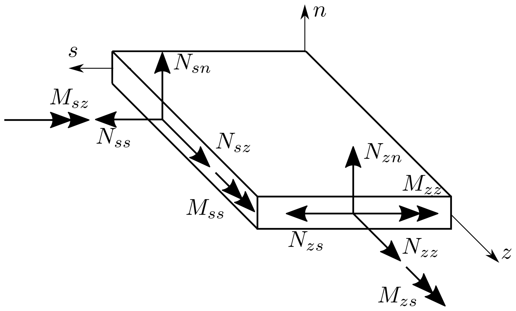
Figure 2Shell forces and moments based on Jung and Nagaraj (2002).
The constitutive relations are semi-inverted to obtain the missing force and moment fluxes (Nzz, Mzz, Mzs) and strains (γzs, κss) from the strains and fluxes for which assumptions are made (displacement-based part: εzz, κzz, κzs; force-based part: Nzs, Mss). For the constitutive relations, it follows that
2.6.3 Determination of Nzs and Mss
Assumption for Nzs and Mss are made in (Jung and Park, 2005, Eq. 13, force-based approach). They are given by the expressions
where , , , and represent the unknown circuit shear fluxes and hoop moments for each cell of a closed multi-cell section. To obtain the continuity condition for each cell of the multi-cell cross-section, four conditions for each cell (Ci) are used and are given by
Herein, Ai is the enclosed area of the respective cell i. After solving this linear system of equations for the given cross-sectional geometry, the variables , , , and are obtained, yielding an expression for Nzs and Mss given by
where and ξa and ξr are the active and reactive parts of the shear flux and hoop moment as defined by Gjelsvik and Hodges (1982).
2.6.4 Cross-sectional stiffness relations
The cross-sectional stiffness relations are subdivided into an active part (denoted by Kbb) and a reactive part (denoted by Kvv and Kbv), which are derived in the following. The active part of the strain energy is considered first. Using the principle of virtual work, the active strain energy related to the virtual strains becomes
Herein, the virtual strains are derived from the virtual cross-sectional displacements δqb. With the help of equation Eq. (11), it is possible to establish a relation between the cross-sectional displacements qb and the corresponding cross-sectional loads given by
where N is the normal force; Mx and My are the bending moments around the x and the y axis, respectively; T is the torsion moment; and Mω is the warping bi-moment.
In order to obtain the shear stiffness terms, a cantilevered beam that is loaded at the tip by shear forces in the x direction, Vx, and the y direction, Vy, is considered following the first-order shear deformation theory. It has to be noted that this case does not represent the wind turbine blade use case. Once the stiffness and mass properties of all cross-sections are calculated, a beam model consisting of several different cross-sections representing the blade certainly needs to be constructed and can subsequently be used to carry out load simulations, obtaining the real load distribution along the blade. Differentiating the cross-sectional load vector Fb with respect to z yields the expression
With denoting the cross-sectional displacements for extension, bending, and torsion, the reactive part of the shear flux ξr can be determined using
The shear forces are calculated with the matrix p, which is defined by
Herein, is the complete vector of the cross-sectional displacements. The matrix p is split in a 2 × 5 left part called p1 and a 2 × 2 right part called p2. Introducing
and
with , the resulting 7 × 7 cross-sectional stiffness matrix K is obtained, which is given by the expression
Substitution into Eq. (1) yields the relationship between the cross-sectional displacements q and the internal loads F. The rows and columns of the matrix K are then rearranged to form the order given in Table 2. This indexing of F, K, and q is used in the following.
Table 2Explanation of the indices of the cross-section stiffness matrix K, the cross-section displacements q, and the internal loads F.

It should be mentioned that the formulation of the kinematics results in a point of attack for extension and bending loads that is located in the origin of the cross-section coordinate system. The point of attack for transversal and torsion loads is the pole (also referred to as shear center); see Fig. 3.
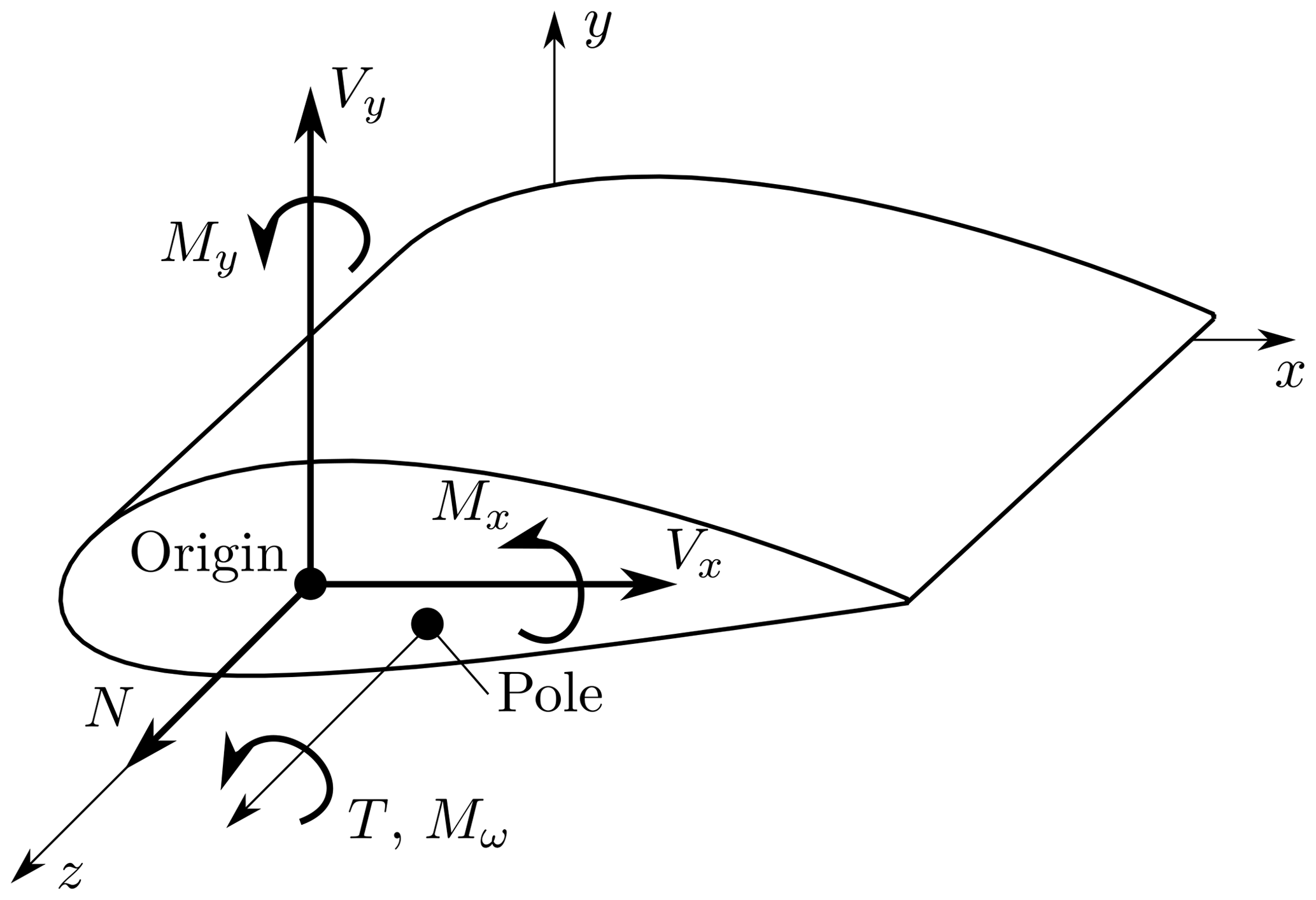

Figure 4Cross-section geometries in PreDoCS for test cases 0–3 (a) and 10–11 (b). BECAS mesh of the left upper corner for test cases 1–3 (c) and front lower web–shell intersection (d).
In this section, the mechanical properties for six different test cases (with two different cross-section geometries) are determined utilizing the three cross-sectional approaches selected in Sect. 2.5. Thereby, the stiffness matrix, the positions of the elastic and the shear center, and the stress distributions across the cross-section are compared with the results of the 2D FE solver BECAS (Blasques, 2012), which serves as a reference. The elastic center is the point where an axial force does not induce bending. The shear center is the point where applied transverse forces do not induce torsional twist. The presented analytical approaches use the origin of the cross-section as the application point for axial forces and bending moments. The transverse forces and torsional moments are applied at the shear center. Both analytical approaches, Song and Jung, require the pole (center of rotation of the cross-section) as input for the kinematic formulations. With the assumption that the center of rotation equals the shear center, the Wiedemann (2007) approach is the only approach that can be used to determine the shear center in advance. In contrast to the analytical approaches, the application point for all the force and moment load of the cross-section for BECAS is the origin. To be able to compare the analytical approaches with BECAS, the origin of the cross-section must coincide with the shear center. This is achieved by translating the cross-section geometry accordingly prior to the analysis. In the case of Song and Jung the shear center can be obtained from the shear stress distribution, as the shear center can also be referred to as the point of attack of the resultant shear force.
Table 3Number of elements of the cross-sections for the different approaches.
3.1 Test cases
The comparison is carried out using two different cross-sections with different material distributions. One cross-section is a thin-walled rectangle (Fig. 4a), allowing a visual verification of expected stress distributions for simple load cases. The second cross-section is a NACA 2412 airfoil with two shear webs at 30 % and 50 % of the chord length, measured from the leading edge, as shown in Fig. 4b. This cross-section is representative of a wind turbine rotor blade. For the distinction between effects caused by the geometry and the material, two material concepts are used: aluminum as an isotropic material ( MPa, ν=0.32) and a composite layup consisting of carbon fiber UD prepreg based on Hexcel T800/M21 ( MPa, MPa, ν12=0.369, ν22=0.5, MPa, t=0.184 mm). The stacking sequence of the webs of the NACA 2412 airfoil is , and all other stacking sequences are . Based on the two cross-sections and the aforementioned materials, the following test cases are created and assigned a unique ID:
Table 4Test case 1 – rectangular cross-section with composite layup.

Table 5Test case 2 – rectangular cross-section with CUS layup.
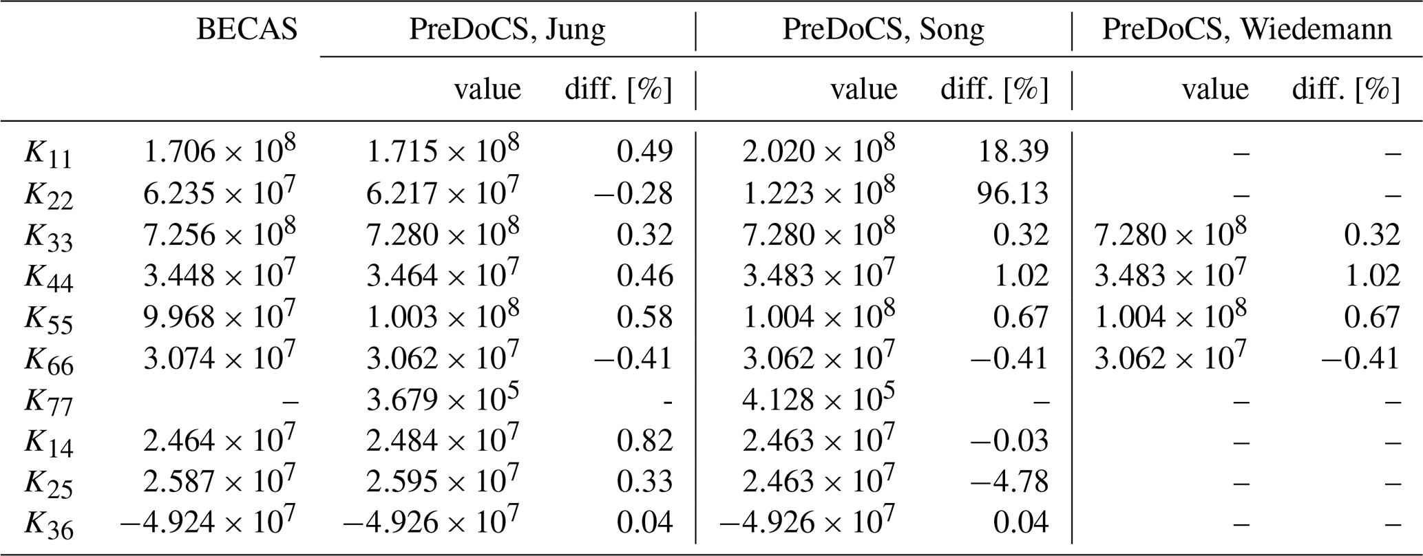
Table 6Test case 3 – rectangular cross-section with CAS layup.

Table 7Test case 11 – NACA 2412 cross-section with composite layup.
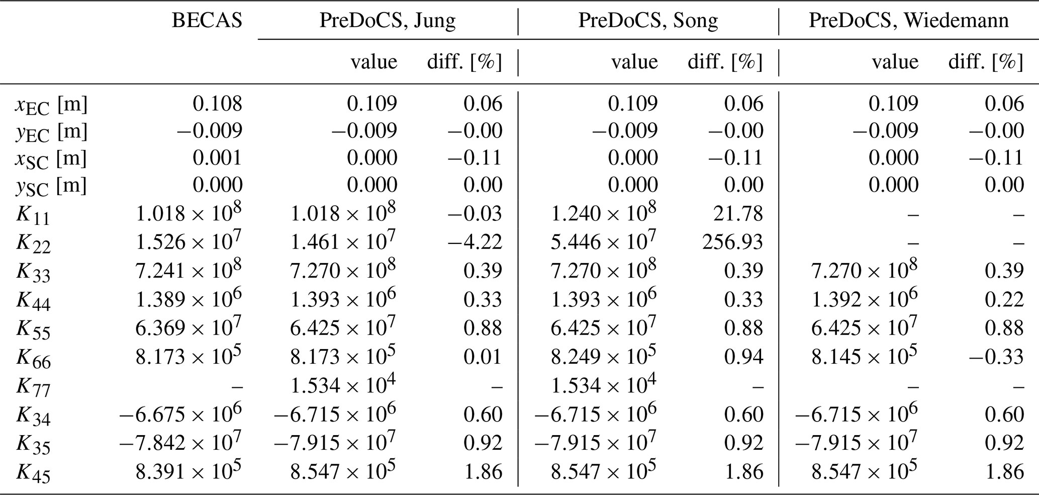
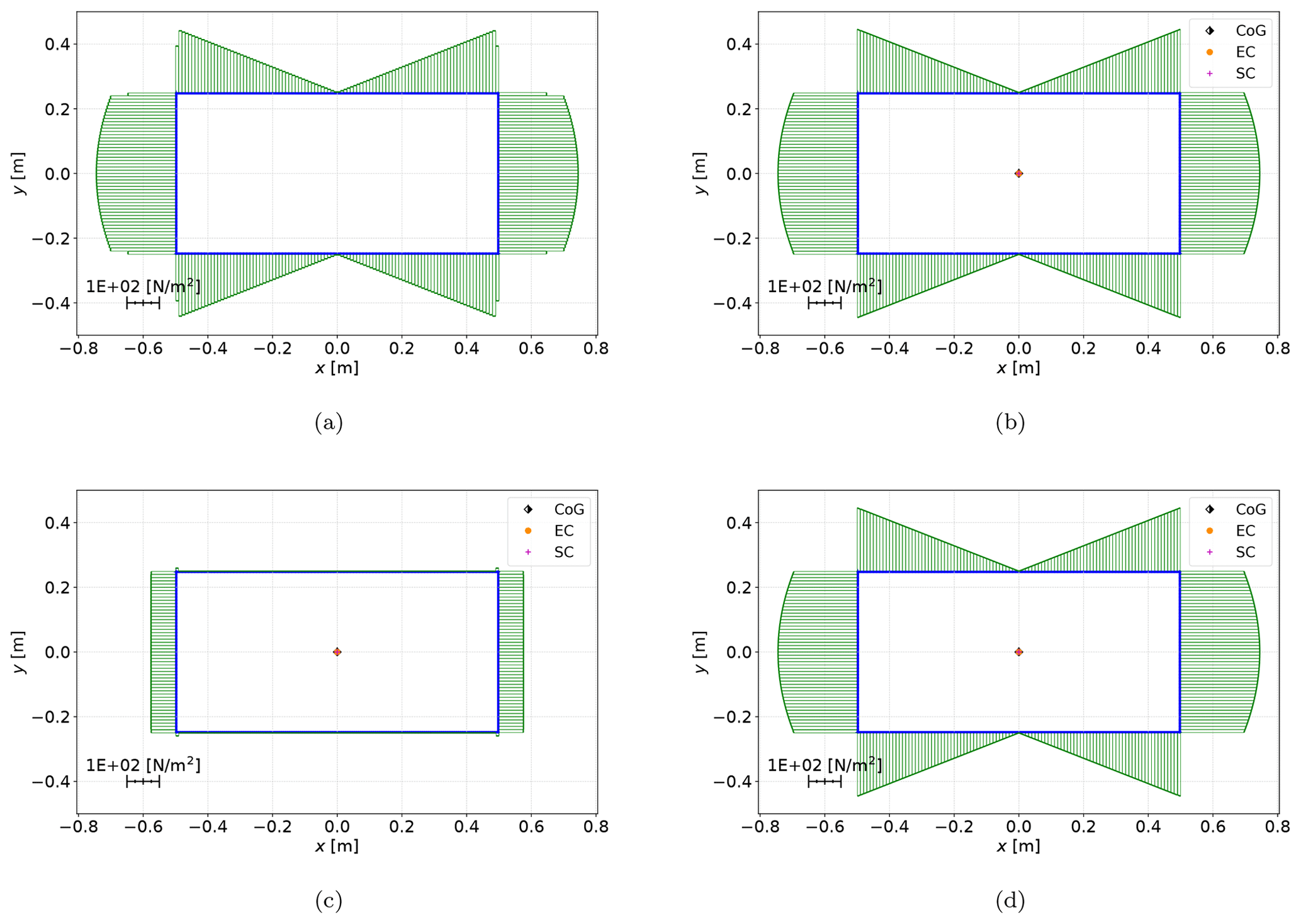
Figure 5Shear stress σzs distribution for test case 0 under a unit transverse force in the y direction for BECAS (a) and PreDoCS approaches of Jung (b), Song (c), and Wiedemann (d).
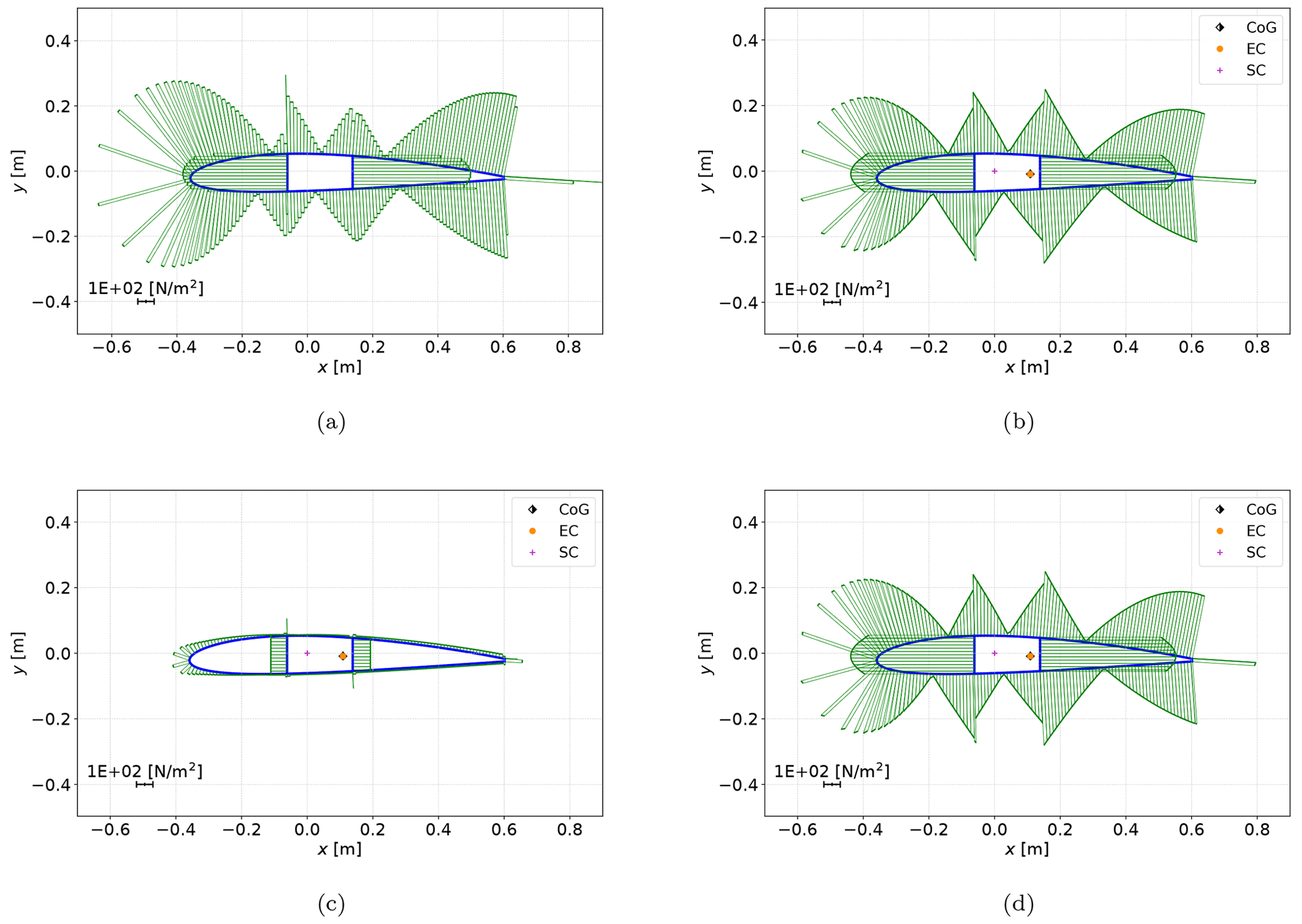
Figure 6Shear stress σzs distribution for test case 10 under a unit transverse force in the y direction for BECAS (a) and PreDoCS approaches of Jung (b), Song (c), and Wiedemann (d).
-
0 – rectangular CS made of 4.416 mm aluminum (same thickness as the composite layup);
-
1 – rectangular CS made of the composite layup described above;
-
2 – rectangular CS made of the composite layup described above rotated by 30° in all walls to get a circumferentially uniform stiffness configuration (CUS, Librescu, 2006, p. 88);
-
3 – rectangular CS made of the composite layup described above rotated by 30°, with walls opposite to each other with a different sign to get a circumferentially asymmetric stiffness configuration (CAS, Librescu, 2006, p. 91);
-
10 – NACA 2412 CS made of 4.416 mm aluminum;
-
11 – NACA 2412 CS made of the composite layups described above.
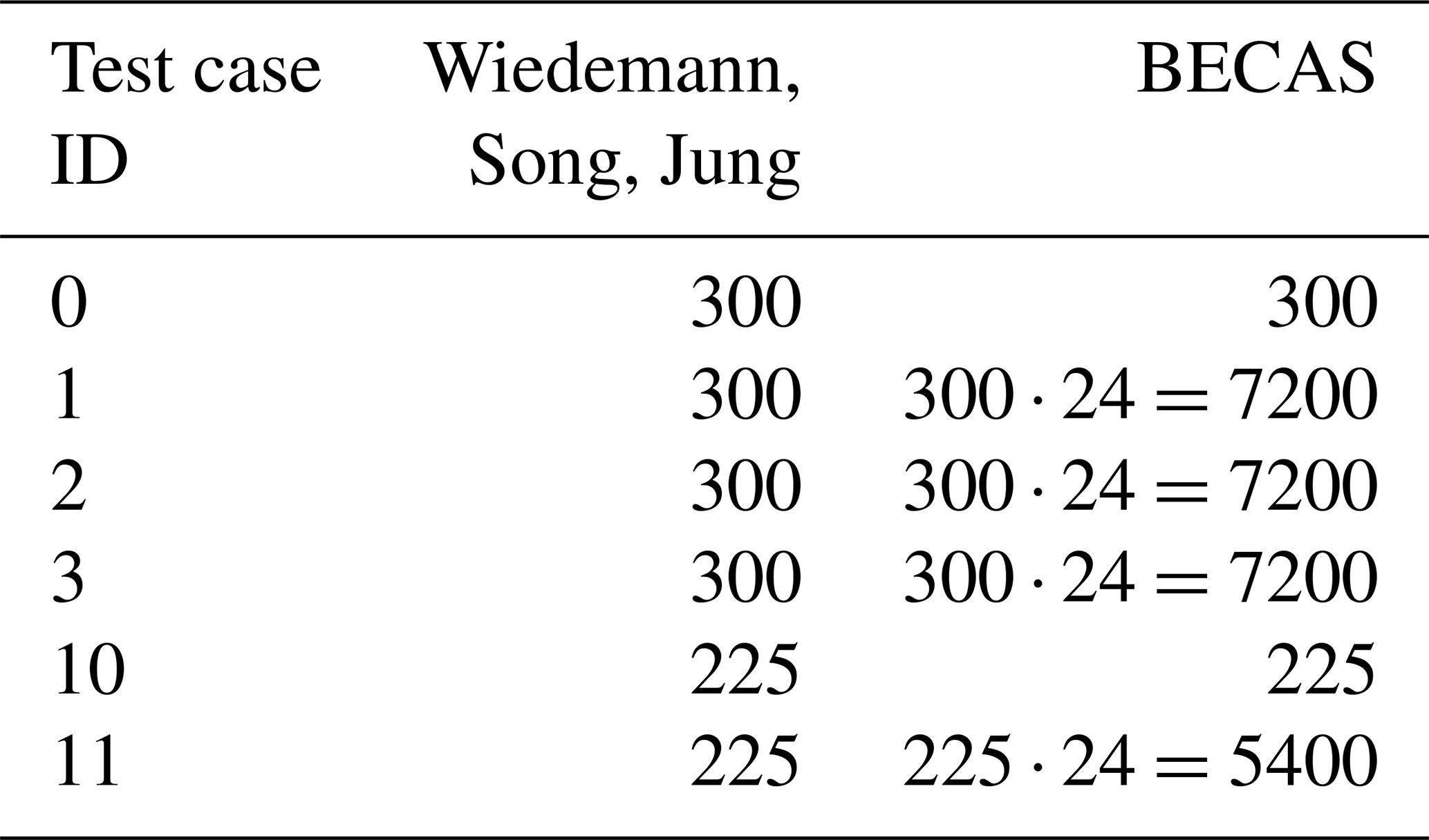
To obtain accurate results for BECAS, a fine mesh and an accurate geometric representation of the cross-section is required (Maes et al., 2024). The contour is discretized in the contour direction similarly for all cross-section calculations based on a mesh convergence study. The rectangular cross-section (0–3) is discretized in the contour direction with 300 equidistant elements of 10 mm length. It should be mentioned that for the rectangular cross-section the analytical approaches are independent of the discretization and already obtain accurate results with a discretization of four elements in the contour direction. A further discretization refinement does not affect the calculation results. Nevertheless, in order to be able to compare element-wise stresses, the same discretization in the contour direction was chosen for the analytical approaches and for BECAS. The airfoil with webs (test cases 10 and 11) is discretized in the contour direction with 225 elements of 10 mm length. The analytical approaches do not need a discretization in the contour thickness direction; BECAS requires a discretization for each layer of the laminate in the contour thickness direction. As the laminates consist of 24 layers, 24 elements are used in thickness direction. The resulting number of elements for the different test cases and the different models are listed in Table 3.
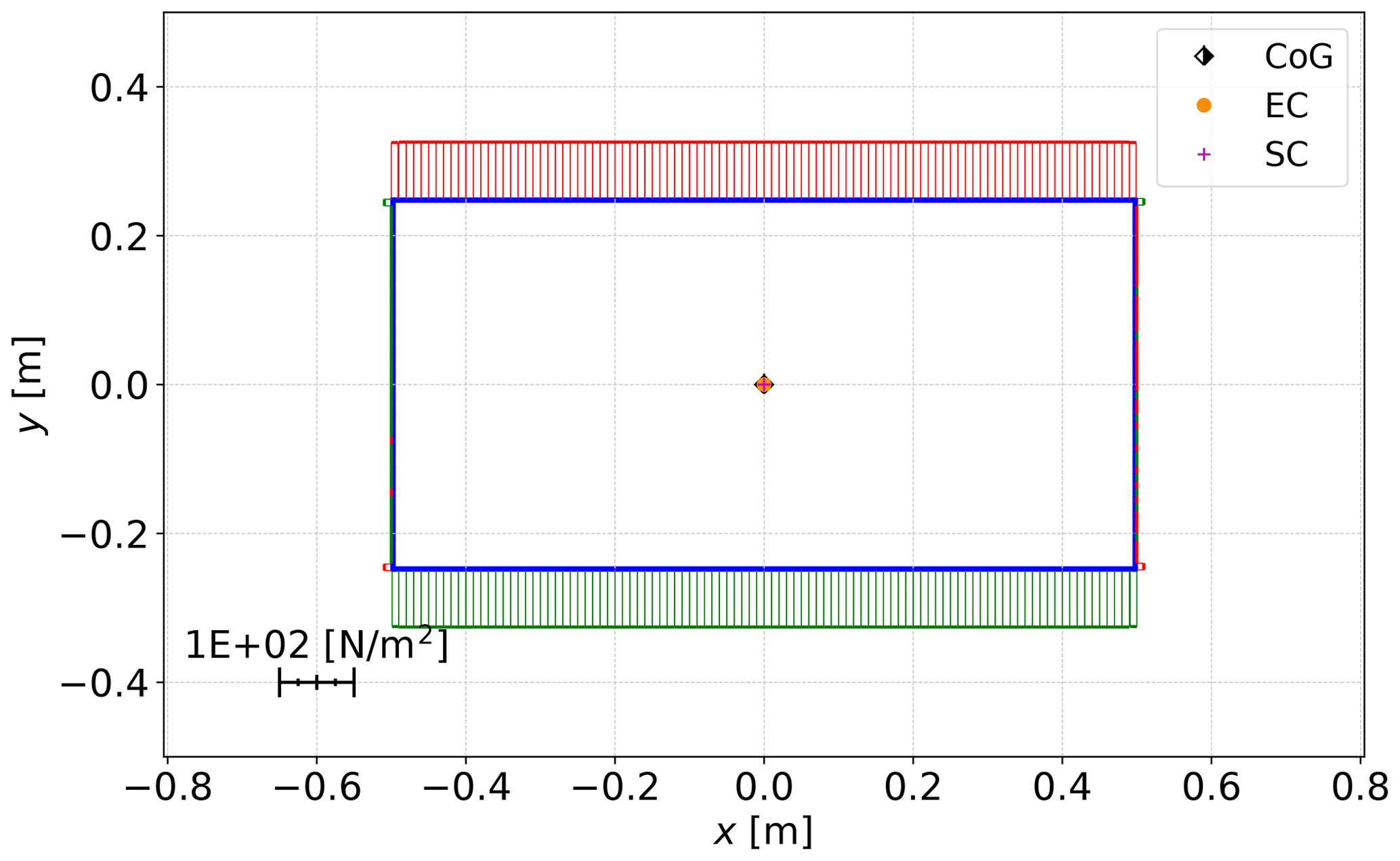
Figure 7Transverse shear stress σzn for test case 0 under a unit transverse force in the y direction (Song approach).
3.2 Stiffness terms
The Tables 4–7 show the non-zero values of the stiffness matrix and, for the test case 11 (NACA 2412 profile), the positions of the elastic (EC) and shear (SC) centers. The indices are according to the description given in Table 2.
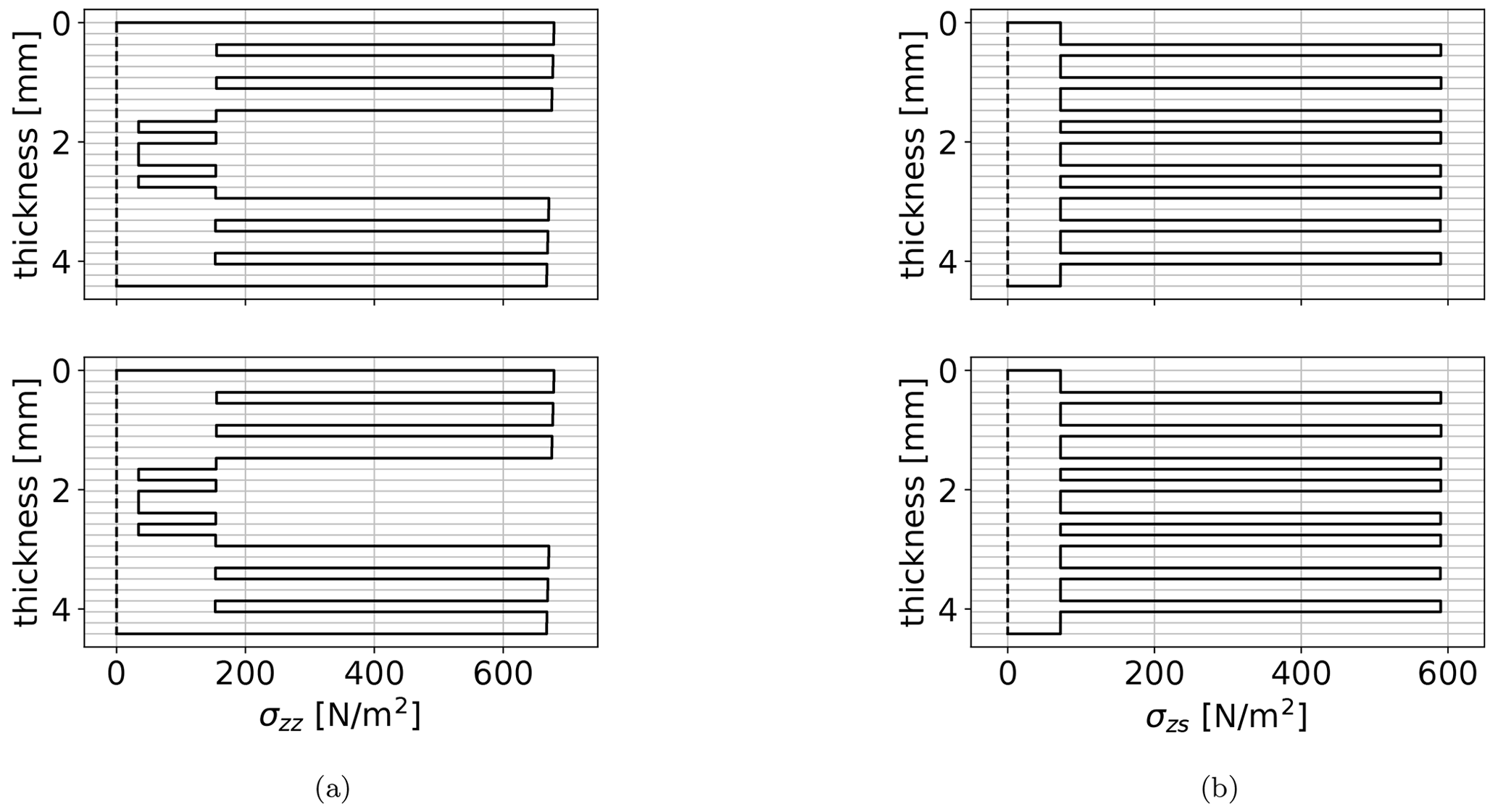
Figure 8Comparison of the stress distribution along the contour thickness between BECAS (top) and Jung (bottom). Normal stress σzz under a unit bending moment around the x axis, evaluated at the center of the upper edge of test case 1 (a). Shear stress σzs under a unit transverse force in the y direction, evaluated at the center of the left web of test case 1 (b).
The shear stiffness terms of Song show high deviations compared to BECAS. In all test cases, deviations around 20 % for K11 and between approximately 100 % and 260 % for K22 can be observed, due to the FSDT used by this approach. The Jung approach shows deviations below 5 %, which indicates a significant improvement. The Wiedemann approach does not cover the shear stiffness terms due to its shear-stiff formulation. The deviations of the main stiffness terms for extension (K33), bending (K44 and K55), and torsion (K66) are below 1 % for the Jung approach. The same applies to the Song and Wiedemann approaches except for test case 3 (CUS layup), where deviations up to 10 % occur, which have to be further investigated. The coupling stiffness terms of the Jung and Song approach show a good accordance with the BECAS results. The stiffness term K36 for extension–torsion coupling of test case 2 (CUS) is calculated almost exactly. The same applies to the stiffness terms K46 and K56 for bend–twist coupling of test case 3 (CAS). Similar to the shear stiffness, the coupling terms are not present in the Wiedemann approach.

Figure 9Boxplots of the median of the relative difference for the active normal and shear stress distributions related to BECAS, grouped by test case (a), grouped by load case (b), and grouped by cross-section theory (c).
The deviations for the elastic and shear center given in Table 7 are well below 1 %. It should be noted that the stiffness terms for restrained warping (terms with index 7) are included in the Song and Jung approach but not available in BECAS. Numerical values for warping stiffness terms of closed cross-sections are not provided in the literature, neither for beam formulations nor for 2D FE approaches where warping is considered as described for the VABS code in Yu et al. (2005). Therefore, a study on the effect of warping at the level of a beam structure needs to be carried out in the future. A comparison of warping displacements and cross-sectional stiffness terms between BECAS and VABS can be found in Blasques (2012).
3.3 Stress distributions
Figures 5 and 6 show a qualitative comparison of the shear stress distributions caused by a transverse force in the y direction. A comparison between the three selected approaches for the test cases 0 (rectangular cross-section) and 10 (NACA 2412 airfoil) is shown. Furthermore, the centers of gravity (CoGs), the elastic centers (ECs), and the shear centers (SCs) are displayed.
The differences between the different approaches in the shear stress distributions can be seen very clearly. The extraordinarily high deviations of the Song approach result from the use of the FSDT, which assumes a constant shear strain over the entire cross-section. The shear stress magnitude using Song's approach is only a third of that using the other approaches. This is caused by Song's assumption that the shear stresses occur in the direction of the contour as well as perpendicular to the contour. Combined with the assumption of the FSDT (constant shear strain over the cross-section) and the isotropic material of test case 0, the horizontal parts of the contour take two-thirds of the transverse force due to their two-thirds share of the total contour length. Hence, the vertical parts carry only one-third due to the same reason. To illustrate the described effect, the transverse shear stress of the Song approach is shown in Fig. 7. The qualitative stress distributions of Jung and Wiedemann show a good agreement with the results from BECAS. Differences in the absolute values can be observed for test case 10 and are discussed later in the qualitative comparison.
Figure 8 shows the comparison of stress distribution along the contour thickness between BECAS (top) and Jung (bottom) of test case 1 (rectangular cross-section with the layup of ). Figure 8a shows the maximum normal stress σzz under a unit bending around the x axis, evaluated at the center of the upper edge of the rectangular cross-section. It can be observed that the 0° plies carry the major portion of the longitudinal load, which is what the 0° plies are included for. Figure 8b shows the maximum shear stress σzs under a unit transverse force in the y direction, evaluated at the center of the left web of the rectangular cross-section. In this case the ±45° plies carry the major portion of the shear loads, which is the purpose of the ±45° plies. Both figures show very good agreement between the BECAS and Jung solutions.
A quantitative comparison was carried out and is shown in Fig. 9. The distributions of σzz and σzs using the analytical approaches are compared with those using BECAS for all test cases and all load cases (transverse force in the x direction and y direction, extension, bending around the x axis and the y axis, torsion). Only the active stresses are considered (σzz for extension and bending; σzs for transverse force and torsion), since the reaction stresses become negligibly small and therefore small absolute differences result in very high relative differences. The goal is to represent the deviation of the stress distribution along the complete contour of the cross-section for one load case and one test case in one single value. Hence, the absolute value of the relative difference was calculated for each element midpoint of the cross-section, so that negative and positive differences do not cancel each other out. From this difference distribution, the median is taken as a comparative value, because it is not strongly influenced by local outliers. The medians of relative differences for all test case–load case combinations are shown in Fig. 9 as boxplots1 grouped by test case, load case, and calculation method.
Figure 9c shows the already mentioned wrongly calculated shear stress distribution under a transverse force with the Song approach (due to the FSDT used therein). The median of the deviations for Jung and Wiedemann are below 1 %. Outliers up to 25 % of the median can be observed for the test cases 10 and 11 displayed in the upper right corner of Fig. 9a. The corresponding load case for the Jung approach is the transverse load in the y direction, shown in Fig. 9b. The shear stress of the analytical approaches is concentrated in the webs rather than in the leading and trailing edge contour compared to BECAS. This effect has to be further investigated.
As already mentioned, for an accurate stress distribution of a rectangular cross-section (as shown in Fig. 5), the analytical approaches require only four elements (one element per edge) and can return the exact stress function along the element or the minimum and maximum values of the element. Due to the FE approach of BECAS, more finite elements are necessary to get a correct stress distribution (see Fig. 5). For cross-sections with segments that are not straight, the analytical approaches also need an accurate geometric representation of the cross-section using several elements, but the stress distribution is exact within one element.
3.4 Performance
Table 8 shows the computation time for the calculation of the cross-sectional properties for BECAS and the three implemented cross-section processors in PreDoCS according to the approaches of Jung, Song, and Wiedemann. Furthermore the computational time for one load case is displayed. All computations include the time for meshing of the cross-sections. For all approaches the same mesh discretization in the contour direction is used (according to Table 3) to be able to compare the stress distributions given in Figs. 5 and 6. The calculations are executed on the same PC (Windows 11, 64-bit, AMD Ryzen 7 5800H, 8 × 3.2–4 GHz, 16 GB RAM). The analytical approaches achieve the same accuracy already with four elements in the contour direction. Further mesh refinement does not affect the stiffness terms and stress distribution. In contrast to that, a fine FE mesh is required in BECAS in order to obtain a converged solution. The resulting benefit by means of computation time savings is shown in the last row of Table 8.
Table 8Comparison of the computation time for the calculation of the cross-sectional properties and one load case, compared to BECAS. The last row compares the calculation of the rectangular cross-section with a four-element mesh for PreDoCS. SD stands for standard deviation.
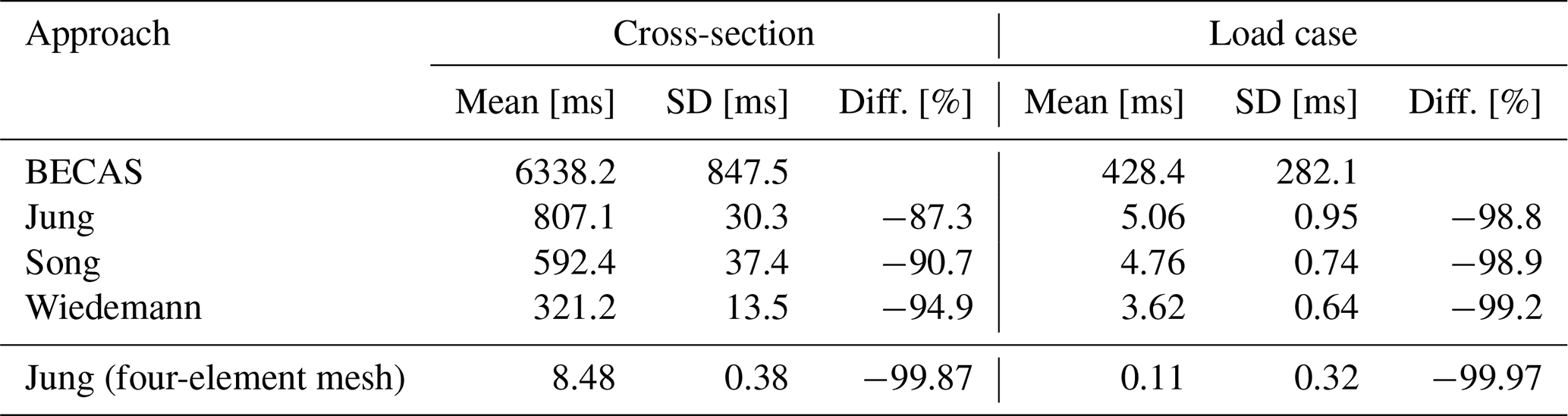
It can be observed that for the cross-sectional calculation the analytical approaches are an order of magnitude (partly even more) faster than BECAS. For a single load case the difference is around 2 orders of magnitude. BECAS uses MATLAB, which has highly optimized functions for matrix calculations, where a further improvement of the performance is difficult. For PreDoCS, code optimization has not been done yet. Using packages such as Cython (Behnel et al., 2011) will further improve the computation performance. Cython provides the option to compile parts of the Python code as native C-like code which can improve the performance significantly.
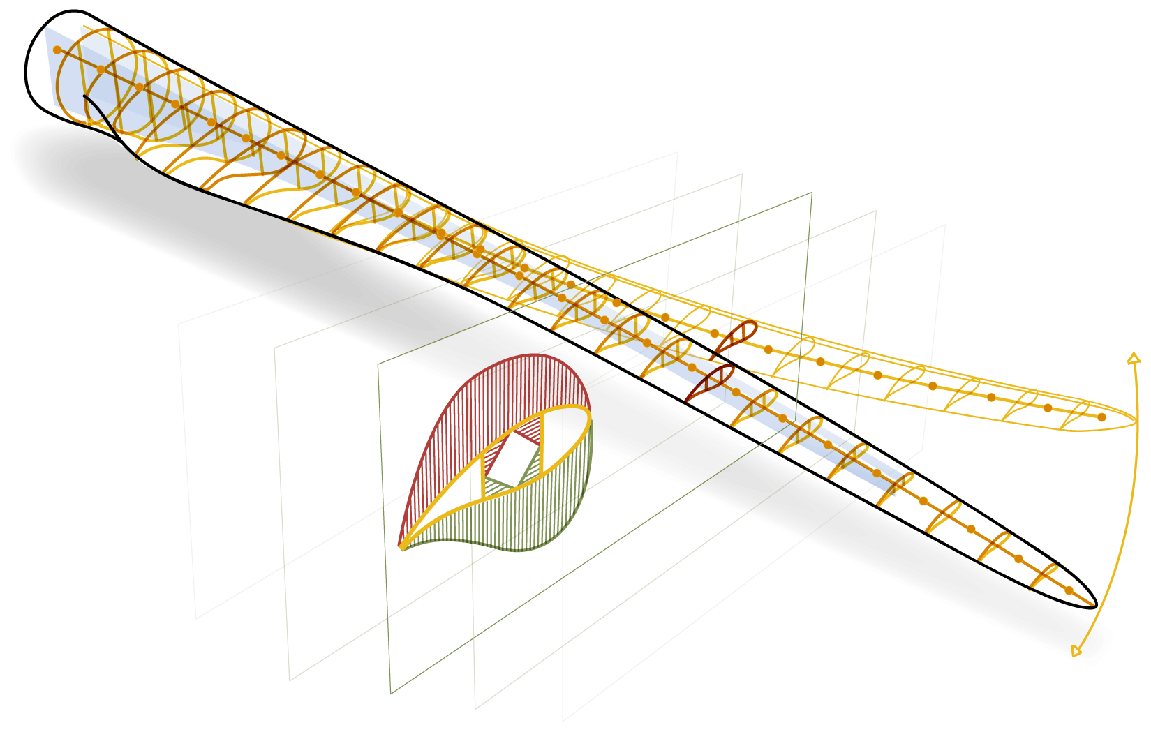
The time savings need to be further analyzed in the context of a design optimization problem for a complete rotor blade modeled as a beam. Thereby the PreDoCS module has to provide the stiffness and stress distributions for multiple cross-sections along the span as shown in Fig. 10 and multiple load cases. The performance improvement per cross-section and load case will therefore add up.
The present paper provides an evaluation of different analytical cross-sectional approaches on the basis of requirements derived for the preliminary design of wind turbine blades. The approaches of Wiedemann, Song, and Jung were used to calculate cross-sectional stiffness matrices and stress distributions across the cross-section. The results were compared to each other and to the 2D FE-based approach of BECAS, which served as a reference.
Since transverse forces play an important role within the design of rotor blades, the Song approach turned out not to be suitable due to the wrongly determined shear stress distribution caused by the use of the FSDT. The shear stiffness terms and the related coupling terms were also not calculated correctly. The Wiedemann approach did not cover the coupling and shear stiffness terms at all. It is a simple and fast approach usable only for determining stress distributions, which show good agreement with the results from BECAS and Jung.
In terms of the accuracy of stiffness terms (also for coupling and shear) and stress distributions, the approach of Jung shows the best results, with deviations to BECAS below 5 % (below in most cases), and is therefore taken as the cross-section processor in PreDoCS. For the stress analyses of test cases 10 and 11, deviations up to 25 % can be observed in Jung's model for transversal load in the y direction, which have to be further investigated. However, it should be noted that the other analytical models do not predict the transverse shear response better.
The comparison of the approaches on the level of a beam structure with respect to overall beam deformations is a work in progress. The effect of warping also needs to be further investigated. In general, the beam model itself must include geometrical non-linearity in the sense of large deflections, as blades undergo very large deflections in operation. Large deflections in turn result in additional coupling effects. For example, when considering equilibrium in the deformed state (which is the definition of geometrical non-linearity), large flap-wise deflections trigger edge-wise bend–twist coupling. If geometric non-linearity were to be involved in the beam theory applied for the calculation of the cross-sectional properties, the structural parameters of the cross-sections would need to be updated in each iteration step of the non-linear beam solution, i.e., in each iteration of each time step in the turbine simulation. This could potentially affect the turbine dynamics, which would be interesting to look at. However, this goes far beyond the scope of this paper and may be the subject of future work. In any case, such an extension would make the turbine simulation very costly, as the number of iterations would increase dramatically.
The presented analytical approaches show a significantly better performance with respect to computational time compared to the 2D FE code BECAS. This underlines the usability of analytical cross-section approaches in PreDoCS as a solver within a design process where many design candidates need to be evaluated and a high number of design iterations occur. The higher resolution of the stress distribution due to its exact and analytical function of the contour coordinate is easy to differentiate analytically, which supports the usage of the approach in gradient-based single- or multi-disciplinary optimization processes with a high number of design variables.
The code is open source and available under the MIT License (Werthen et al., 2023, https://doi.org/10.5281/zenodo.10305952). The simulation results of this paper can be reproduced with the code.
EW and DH developed the methodology and software, did the analyses and wrote the manuscript. CB and CH revised the manuscript and provided scientific supervision.
The contact author has declared that none of the authors has any competing interests.
Publisher’s note: Copernicus Publications remains neutral with regard to jurisdictional claims made in the text, published maps, institutional affiliations, or any other geographical representation in this paper. While Copernicus Publications makes every effort to include appropriate place names, the final responsibility lies with the authors.
We would like to thank the Technical University of Denmark (DTU) for providing BECAS.
The work presented in this paper was funded by the Deutsche Forschungsgemeinschaft (DFG, German Research Foundation) under Germany's Collaborative Research Center, CRC 1463/1, “Integrated design and operation methodology for offshore megastructures”, project ID 434502799.
The article processing charges for this open-access publication were covered by the German Aerospace Center (DLR).
This paper was edited by Julie Teuwen and reviewed by Alexander Krimmer and two anonymous referees.
Behnel, S., Bradshaw, R., Citro, C., Dalcin, L., Seljebotn, D. S., and Smith, K.: Cython: The best of both worlds, Comput. Sci. Eng., 13, 31–39, https://doi.org/10.1109/MCSE.2010.118, 2011. a
Bir, G. S.: User's Guide to PreComp (Pre-Processor for Computing Composite Blade Properties), National Renewable Energy Laboratory, https://doi.org/10.2172/876556, 2006. a
Blasques, J.: User's Manual for BECAS: A cross section analysis tool for anisotropic and inhomogeneous beam sections of arbitrary geometry, no. 1785(EN) in Denmark, Forskningscenter Risoe, Risoe-R, Risø DTU – National Laboratory for Sustainable Energy, https://orbit.dtu.dk/en/publications/9a623506-af47-41d6-9d24-5ef0e5b762c1 (last access: 30 March 2024), 2012. a, b, c, d, e, f
Borri, M., Ghiringhelli, G. L., and Merlini, T.: Composite Beam Analysis Linear Analysis of Naturally Curved and Twisted Anisotropic Beams, United States Army, European Research Office of the US army, http://www.dtic.mil/dtic/tr/fulltext/u2/a252652.pdf (last access: 30 March 2024), 1992. a
Bottasso, C., Campagnolo, F., Croce, A., and Tibaldi, C.: Optimization-based study of bend-twist coupled rotor blades for passive and integrated passive/active load alleviation, Wind Energy, 16, 1149–1166, https://doi.org/10.1002/we.1543, 2012. a
Carrera, E. and Petrolo, M.: Refined beam elements with only displacement variables and plate/shell capabilities, Meccanica, 47, 537–556, https://doi.org/10.1007/s11012-011-9466-5, 2011. a
Chandra, R. and Chopra, I.: Structural behavior of two-cell composite rotor blades with elastic couplings, AIAA J., 30, 2914–2921, https://doi.org/10.2514/3.11637, 1992. a, b, c, d
Chen, H., Yu, W., and Capellaro, M.: A critical assessment of computer tools for calculating composite wind turbine blade properties, Wind Energy, 13, 497–516, https://doi.org/10.1002/we.372, 2010. a
Deo, A. and Yu, W.: Thin-walled composite beam cross-sectional analysis using the mechanics of structure genome, Thin Wall. Struct., 152, 106663, https://doi.org/10.1016/j.tws.2020.106663, 2020. a
Dugas, M.: Ein Beitrag zur Auslegung von Faserverbundtragflügeln im Vorentwurf, Universität Stuttgart, https://doi.org/10.18419/opus-3672, 2002. a
Gasch, R. and Twele, J.: Wind Power Plants: Fundamentals, Design, Construction and Operation, Springer Berlin Heidelberg, Berlin, Heidelberg, 2nd edn., ISBN 978-3-642-22937-4, 2012. a
Giavotto, V., Borri, M., Mantegazza, P., Ghiringhelli, G., Carmaschi, V., Maffioli, G. C., and Mussi, F.: Anisotropic beam theory and applications, Comput. Struct., 16, 403–413, https://doi.org/10.1016/0045-7949(83)90179-7, 1983. a
Gjelsvik, A. and Hodges, D. H.: The Theory of Thin-Walled Bars, J. Appl. Mech., 49, 468–468, https://doi.org/10.1115/1.3162198, 1982. a
Hodges, D. H.: Nonlinear composite beam theory, American Institute of Aeronautics and Astronautics, American Institute of Aeronautics and Astronautics, Inc., ISBN 978-1-56347-697-6, https://doi.org/10.2514/4.866821, 2006. a, b, c, d, e, f
Johnson, E. R., Vasiliev, V. V., and Vasiliev, D. V.: Anisotropic Thin-Walled Beams with Closed Cross-Sectional Contours, AIAA J., 39, 2389–2393, https://doi.org/10.2514/2.1247, 2001. a, b, c
Jung, S. and Nagaraj, V. T.: Structural Behavior of Thin- and Thick-Walled Composite Blades with Multi-Cell Sections, in: 43rd AIAA/ASME/ASCE/AHS/ASC Structures, Structural Dynamics, and Materials Conference, American Institute of Aeronautics and Astronautics, Reston, Virigina, ISBN 978-1-62410-117-5, https://doi.org/10.2514/6.2002-1432, 2002. a, b, c, d, e, f, g
Jung, S., Kim, C.-J., Ko, J. H., and Kim, C.-W.: Theory of Thin-Walled, Pretwisted Composite Beams with Elastic Couplings, Adv. Compos. Mater., 18, 105–119, https://doi.org/10.1163/156855109X428736, 2009. a
Jung, S. N. and Park, I. J.: Structural Behavior of Thin- and Thick-Walled Composite Blades with Multicell Sections, American Institute of Aeronautics and Astronautics Journal, 43, 572–581, https://doi.org/10.2514/1.12864, 2005. a
Jung, S. N., Nagaraj, V. T., and Chopra, I.: Refined Structural Model for Thin- and Thick-Walled Composite Rotor Blades, AIAA J., 40, 105–116, https://doi.org/10.2514/2.1619, 2002. a, b, c
Kim, C. and White, S. R.: Thick-walled composite beam theory including 3-d elastic effects and torsional warping, Int. J. Solids Struct., 34, 4237–4259, https://doi.org/10.1016/S0020-7683(96)00072-8, 1997. a
Kollár, L. P. and Springer, G. S.: Mechanics of Composite Structures, Cambridge University Press, ISBN 9780511547140, https://doi.org/10.1017/cbo9780511547140, 2003. a, b, c
Lee, J.: Flexural analysis of thin-walled composite beams using shear-deformable beam theory, Compos. Struct., 70, 212–222, https://doi.org/10.1016/j.compstruct.2004.08.023, 2005. a
Lee, S.-L. and Shin, S. J.: Structural design optimization of a wind turbine blade using the genetic algorithm, Eng. Optimiz., 54, 2053–2070, https://doi.org/10.1080/0305215X.2021.1973450, 2022. a
Libove, C.: Stresses and rate of twist in single-cell thin-walled beams with anisotropic walls, AIAA J., 26, 1107–1118, https://doi.org/10.2514/3.10018, 1988. a, b, c
Librescu, L.: Thin-walled composite beams: Theory and application, Springer Link Bücher, vol. 131, Springer Netherlands, Dordrecht, ISBN 9781402042034, https://doi.org/10.1007/1-4020-4203-5, 2006. a, b, c
Librescu, L. and Song, O.: Behavior of thin-walled beams made of advanced composite materials and incorporating non-classical effects, Appl. Mech. Rev., 44, S174, https://doi.org/10.1115/1.3121352, 1991. a
Maes, V. K., Macquart, T., Weaver, P. M., and Pirrera, A.: Sensitivity of cross-sectional compliance to manufacturing tolerances for wind turbine blades, Wind Energ. Sci., 9, 165–180, https://doi.org/10.5194/wes-9-165-2024, 2024. a
Mansfield, E. H. and Sobey, A. J.: The Fibre Composite Helicopter Blade, Aeronaut. Quart., 30, 413–449, https://doi.org/10.1017/S0001925900008623, 1979. a, b, c
Qin, Z. and Librescu, L.: On a shear-deformable theory of anisotropic thin-walled beams: Further contribution and validations, Compos. Struct., 56, 345–358, https://doi.org/10.1016/S0263-8223(02)00019-3, 2002. a
Rehfield, L. W., Atilgan, A. R., and Hodges, D. H.: Nonclassical Behavior of Thin-Walled Composite Beams with Closed Cross Sections, J. Am. Helicopter Soc., 35, 42–50, https://doi.org/10.4050/JAHS.35.42, 1990. a, b, c
Rosemeier, M. and Krimmer, A.: Rotorblattstruktur, in: Einführung in die Windenergietechnik, edited by: Schaffarczyk, A. P., Chap. 5, Carl Hanser Verlag GmbH & Co. KG, 3 edn., 169–220, ISBN 9783446473225, https://doi.org/10.1007/978-3-446-47322-5, 2022. a
Saravia, M.: Calculation of the Cross Sectional Properties of Large Wind Turbine Blades, Mecánica Computacional, 54, 3619–3635, http://www.cimec.org.ar/ojs/index.php/mc/issue/view/876 (last access: 30 March 2024), 2016. a
Saravia, M. C., Saravia, L. J., and Cortínez, V. H.: A one dimensional discrete approach for the determination of the cross sectional properties of composite rotor blades, Renew. Energ., 80, 713–723, https://doi.org/10.1016/j.renene.2015.02.046, 2015. a, b
Scott, S., Macquart, T., Rodriguez, C., Greaves, P., McKeever, P., Weaver, P., and Pirrera, A.: Preliminary validation of ATOM: an aero-servo-elastic design tool for next generation wind turbines, J. Phys. Conf. Ser., 1222, 012012, https://doi.org/10.1088/1742-6596/1222/1/012012, 2019. a, b
Scott, S., Greaves, P., Weaver, P. M., Pirrera, A., and Macquart, T.: Efficient structural optimisation of a 20 MW wind turbine blade, J. Phys. Conf. Ser., 1618, 042025, https://doi.org/10.1088/1742-6596/1618/4/042025, 2020. a
Serafeim, G. P., Manolas, D. I., Riziotis, V. A., Chaviaropoulos, P. K., and Saravanos, D. A.: Optimized blade mass reduction of a 10 MW-scale wind turbine via combined application of passive control techniques based on flap-edge and bend-twist coupling effects, J. Wind Eng. Ind. Aerod., 225, 105002, https://doi.org/10.1016/j.jweia.2022.105002, 2022. a
Song, O.: Modeling and response analysis of thin-walled beam structures constructed of advanced composite materials, PhD thesis, https://vtechworks.lib.vt.edu/bitstream/10919/38952/1/LD5655.V856_1990.S665.pdf (last access: 30 March 2024), 1990. a, b, c, d
Suresh, J. K. and Nagaraj, V. T.: Higher-order shear deformation theory for thin-walled composite beams, J. Aircraft, 33, 978–986, https://doi.org/10.2514/3.47044, 1996. a
Vo, T. P. and Lee, J.: Flexural–torsional behavior of thin-walled composite box beams using shear-deformable beam theory, Eng. Struct., 30, 1958–1968, https://doi.org/10.1016/j.engstruct.2007.12.003, 2008. a
Wanke, G., Bergami, L., Zahle, F., and Verelst, D. R.: Redesign of an upwind rotor for a downwind configuration: design changes and cost evaluation, Wind Energ. Sci., 6, 203–220, https://doi.org/10.5194/wes-6-203-2021, 2021. a
Weisshaar, T. A.: Aeroelastic Stability and Performance Characteristics of Aircraft with Advanced Composite Sweptforward Wing Structures, Defence Technical Information Center, https://apps.dtic.mil/sti/citations/ADB032318 (last access; 30 March 2024), 1978. a
Werthen, E., Hardt, D., and Hühne, C.: PreDoCS: Preliminary Design of Composite Structures, Zenodo [code], https://doi.org/10.5281/zenodo.10305952, 2023. a
Wiedemann, J.: Leichtbau: Elemente und Konstruktion, Klassiker der Technik, Springer-Verlag, Berlin, Heidelberg, 3rd edn., ISBN 3-540-33656-7, https://doi.org/10.1007/978-3-540-33657-0, 2007. a, b, c, d
Yu, W.: Efficient High-Fidelity Simulation of Multibody Systems with Composite Dimensionally Reducible Components, J. Am. Helicopter Soc., 52, 49–57, https://doi.org/10.4050/JAHS.52.49, 2007. a, b, c
Yu, W., Hodges, D. H., Volovoi, V. V., and Fuchs, E. D.: A generalized Vlasov theory for composite beams, Thin Wall. Struct., 43, 1493–1511, https://doi.org/10.1016/j.tws.2005.02.003, 2005. a, b
A boxplot is a graphical representation of data that gives a good overview of the location and scatter of that data. The boxplots used in this paper contain the following statistical data: median, orange line in the box; interquartile range, box; 1.5 times the interquartile range, “antennae”; and outliers, circles.
We provide a comprehensive overview showing available cross-sectional approaches and their properties in relation to derived requirements for the design of composite rotor blades. The Jung analytical approach shows the best results for accuracy of stiffness terms (coupling and transverse shear) and stress distributions. Improved performance compared to 2D finite element codes could be achieved, making the approach applicable for optimization problems with a high number of design variables.
We provide a comprehensive overview showing available cross-sectional approaches and their...