A large-eddy simulation (LES) model for wind-farm-induced atmospheric gravity wave effects inside conventionally neutral boundary layers

The interaction of large wind farm clusters with the thermally stratified atmosphere has emerged as an important physical process that impacts the productivity of wind farms. Under stable conditions, this interaction triggers atmospheric gravity waves (AGWs) in the free atmosphere due to the vertical displacement of the atmospheric boundary layer (ABL) by the wind farm. AGWs induce horizontal pressure gradients within the ABL that alter the wind speed distribution within the farm, influencing both wind farm power generation and wake development. Additional factors, such as the growth of an internal boundary layer originating from the wind farm entrance and increased turbulence due to the wind turbines, further contribute to wake evolution. Recent studies have highlighted the considerable computational cost associated with simulating gravity wave effects within large-eddy simulations (LESs), as a significant portion of the free atmosphere must be resolved due to the large vertical spatial scales involved. Additionally, specialized boundary conditions are required to prevent wave reflections from contaminating the solution. In this study, we introduce a novel methodology to model the effects of AGWs without extending the LES computational domain into the free atmosphere. The proposed approach addresses the wave reflection problem inherently, eliminating the need for these specialized boundary conditions. We utilize the recently developed multi-scale coupled (MSC) model of Stipa et al. (2024b) to estimate the vertical ABL displacement triggered by the wind farm, and we apply the deformation to the domain of an LES that extends only to the inversion layer. The accuracy in predicting the AGW-induced pressure gradients is equivalent to the MSC model. The AGW modeling technique is verified for two distinct free-atmosphere stability conditions by comparing it to the traditional approach in which AGWs are fully resolved using a domain that extends several kilometers into the free atmosphere. The proposed approach accurately captures AGW effects on the row-averaged thrust and power distribution of wind farms while demanding 12.7 % of the computational resources needed for traditional methods. Moreover, when conventionally neutral boundary layers are studied, there is no longer a need to solve the potential temperature equation, as stability is neutral within the boundary layer. The developed approach is subsequently used to compare the global blockage and pressure disturbances obtained from the simulated cases against a solution characterized by zero boundary layer displacement, which represents the limiting case of very strong stratification above the boundary layer. This approximation, sometimes referred to as the “rigid lid”, is compared against the full AGW solution using the MSC model. This is done for different values of inversion strength and free atmosphere lapse rate, evaluating the ability of the “rigid lid” to predict blockage, wake effects, and overall wind farm performance.

1 Introduction

Wind farms, especially those situated offshore, are increasing both in number and in size and are interacting with the atmosphere well beyond their physical boundaries. Such interactions play an important role in both the evolution of cluster wakes and the amount of flow deceleration experienced upstream, also known as blockage. On the one hand, wind farm wake recovery is greatly influenced by surface stability within the atmospheric boundary layer (ABL). On the other hand, the stably stratified free atmosphere leads to the generation of atmospheric gravity waves (AGWs) when mean flow streamlines are vertically perturbed by the wind farm. These waves exist in the form of interface waves within the capping inversion layer and internal gravity waves aloft, introducing a pressure feedback mechanism at the wind farm scale that ultimately impacts the flow dynamics inside the ABL (Smith, 2010). In contrast to terrain-generated gravity waves (Smith, 1980, 2007; Teixeira, 2014), gravity waves triggered by wind farms yield lower-pressure and lower-velocity perturbations inside the ABL when these are compared against turbulent fluctuations. Moreover, similarly to mountain waves, wind-farm-induced AGWs are characterized by horizontal and vertical wavelengths of 𝒪(10) km, depending on the wind farm length, specific potential-temperature structure, and geostrophic wind. These aspects make AGW observation and experimental measurement difficult to achieve. Because of such complexities, wind-farm-induced AGWs have mainly been studied by means of high-fidelity models such as large-eddy simulations (LESs) or using linear gravity wave theory (Nappo, 2012; Lin, 2007). LESs of AGWs suffer from a high computational cost and AGW reflections at the numerical boundaries. The aim of this study is to overcome these difficulties by using a reduced-order model based on linear theory to construct an LES methodology that significantly simplifies the inclusion of AGW effects within the ABL flow.

Using a two-dimensional numerical model, the impact of gravity waves on the flow around hills and complex terrain was first studied by Klemp and Lilly (1978), who addressed the problem of wave reflection from the upper boundary. Later, wind-farm-induced AGWs were investigated using LES for conventionally neutral boundary layers (CNBLs) by Allaerts and Meyers (2017), Lanzilao and Meyers (2022, 2024), and Stipa et al. (2024b), among others. CNBLs are characterized by neutral stratification within the ABL followed by a positive potential temperature jump Δθ across the inversion layer and a linear lapse rate γ in the free atmosphere aloft. These studies showed that the presence of AGWs has two main implications, namely an adverse pressure gradient upwind of the wind farm, which is responsible for global blockage, and a favorable pressure gradient inside the wind farm, which is beneficial for wake recovery. Moreover, Centurelli et al. (2021) and Maas (2023) showed that LES results strongly differ from reduced-order wake models when thermal stratification is considered. To assess the impact of inversion height, strength, and lapse rate on wind farm blockage and wind farm efficiency in general, Lanzilao and Meyers (2024) conducted an LES parametric study, concluding that the overall effect of AGWs on wind farm performance can be either beneficial or detrimental, depending on the specific structure of the potential temperature profile. This result highlights the importance of including AGWs when modeling wind farms in both high-fidelity and low-fidelity models.

An important aspect that emerges from the above studies, highlighted by Lanzilao and Meyers (2024), is that LESs of wind farms that include AGWs are challenging. Firstly, they are rendered computationally intense by the domain size required to spatially resolve AGWs. Furthermore, special boundary conditions should be used to damp out AGWs before they reach the domain boundaries and reflect, contaminating the solution. To overcome this issue, different approaches have been proposed. Béland and Warn (1975) and Bennett (1976) constructed transient radiation boundary conditions using the Laplace transform, but these require the storage of the entire flow history at each reflecting boundary. Klemp and Durran (1983) overcame this limitation by deriving a radiation condition for the top boundary that is local in time, using the linear hydrostatic Boussinesq equations. The authors also showed that low AGW reflectivity is still observed when these hypotheses are not strictly met, a result that was later confirmed by Lanzilao and Meyers (2023). Another approach that avoids AGW reflections at the top boundary is the so-called Rayleigh damping layer (Klemp and Lilly, 1978). This is a region of the domain where the momentum equation features an extra source term that is proportional to the difference between the perturbed and unperturbed ABL states. In theory, this eliminates AGWs before they can reach the boundary, but the proportionality coefficient, which increases with height, should be properly tuned. Reflections may still be observed when damping is too strong or when it is too weak. In the first case, the Rayleigh damping region behaves as a physical boundary, while in the latter, the damping is insufficient to cancel out perturbations before they reach the physical boundary.

Some guidelines on how to choose the Rayleigh damping parameters have been provided by Lanzilao and Meyers (2023) and Klemp and Lilly (1978). Moreover, many other studies (see Allaerts and Meyers, 2017, 2018, among others) agree that the Rayleigh damping layer located at the top should be larger than the expected vertical wavelength of the AGWs, estimated as ${\mathit{\lambda }}_z=\mathrm{2}\mathit{\pi }G/N$, where N is the Brunt–Väisälä frequency and G is the geostrophic wind. Similarly, the vertical extent of the free atmosphere included within the simulation domain must allow at least one vertical wavelength to be resolved.

Non-reflecting boundaries are also required in the horizontal directions, but their implementation is complicated by the fact that they should not alter the incoming ABL turbulence. In this case, two options are possible. The first is the so-called fringe region technique (Inoue et al., 2014), which is essentially a Rayleigh damping layer where the unperturbed state used to compute the momentum source term is local in both time and space. This requires a separate simulation of the unperturbed flow, referred to as the concurrent precursor, to run concurrently with the main simulation, i.e., the successor. This ensures that a time-resolved and spatially resolved reference turbulent flow is available within the fringe region to compute the damping source at each iteration. As the concurrent precursor naturally contains the incoming turbulence, this technique eliminates AGWs while simultaneously prescribing the unperturbed turbulent inflow to the successor simulation. Similarly to the Rayleigh damping layer, the fringe region requires ad hoc tuning of the proportionality coefficient that controls the amount of damping, which is usually accomplished by trial and error, further raising computational costs. Notably, Lanzilao and Meyers (2023) observed that the fringe region itself may trigger spurious gravity waves while attempting to restore the unperturbed state, requiring an additional layer in which horizontal advection of vertical momentum is suppressed to prevent these spurious perturbations from being transported downstream. Another possibility for avoiding wave reflections at the inlet and outlet boundaries is to use Rayleigh damping regions above the boundary layer (Mehtab Ahmed Khan, personal communication, 2023), so that turbulence remains unaffected below. However, this technique requires the accurate selection of the horizontal unperturbed flow in the free atmosphere and poses issues when a capping inversion layer is present.

Regarding the description of AGWs by means of reduced-order models, this was first achieved by Smith (1980, 2007) for the flow around terrain features in what is referred to as the two-layer model (2LM). The 2LM exploits the linear theory for interacting gravity waves and boundary layers and was later extended to wind farms immersed in CNBLs (Smith, 2010). Building on his work, Allaerts and Meyers (2019) developed the three-layer model (3LM), a substantial improvement of the 2LM, characterized by extra features such as the Coriolis force, the additional wind farm layer that relaxes Smith's homogeneous vertical mixing assumption, and the wind farm–gravity wave coupling mechanism. Although the 3LM was the first model to incorporate AGW effects into predictions of wind farm power losses, it lacked local coupling between the mesoscale and turbine scales, thus failing to address the effects of gravity-wave-induced pressure gradients inside the wind farm and in the wake. Recently, Devesse et al. (2023) and Stipa et al. (2024b) proposed new localized coupling strategies between the 3LM and conventional wake models that capture all features of the interaction of wind farms with AGWs under CNBLs. The latter, referred to as the multi-scale coupled model (MSC), is characterized by a lower computational cost, and its formulation is independent of the adopted wake model.

When thermal stratification above the ABL is very strong, lapse rate and inversion strength lose importance, and the background pressure gradient is mainly determined by the boundary layer height. In this case, the flow cannot be perturbed vertically because thermal stratification acts as a lid located at the ABL top. Such an idealized limiting case is commonly referred to as the rigid lid approximation (Smith, 2024). As the lid imposes zero mean vertical mass flux, the solution is characterized by a harmonic perturbation pressure that renders the mean flow horizontally divergence free, with maximum and minimum pressure at the wind farm start and exit, respectively. The rigid lid approximation maintains some properties of the full gravity wave solution, such as the presence of global blockage and flow acceleration within the wind farm. This, combined with its inherently simpler formulation than the full AGW solution, makes the rigid lid approximation worth investigating for its potential use in engineering parametrizations.

The methodology proposed in this study allows the modeling of AGW effects within a wind farm LES while eliminating the computational burden associated with resolving internal and interfacial waves above the ABL. In fact, while LES is used below the inversion layer, AGWs in the free atmosphere and within the inversion layer are modeled through the MSC model (Stipa et al., 2024b), using the vertical ABL displacement as the coupling variable. As a consequence, the developed approach only requires a vertical domain size that is equal to the height of the inversion layer, which is assumed to coincide with the ABL height. Moreover, no damping regions are needed, as the large-scale pressure gradients produced by AGWs are modeled without resolving the actual waves. Finally, when dealing with CNBLs, the flow is neutral within the boundary layer, and the solution of the potential temperature equation can be omitted. Although the proposed method could be applied in principle to internally stable ABLs by solving for the potential temperature equation, the accuracy of the MSC model – on which the LES solution depends – has not been tested under this condition yet. Hence, this article solely focuses on CNBLs, leaving internal ABL stability as an object for future investigation.

The present paper is organized as follows. Section 2 describes the proposed LES methodology, pointing out its differences with respect to the conventional approach used to simulate the wind farm–gravity wave interaction. Section 3 describes the setup of the LES cases used to verify the proposed methodology. Model verification is presented in Sect. 4, together with an analysis regarding the implications of using the rigid lid approximation. Finally, Sect. 5 highlights the conclusions of the present study.

2 LES methodology

For the LES simulations presented in this paper, we use the open-source finite-volume code TOSCA (Toolbox fOr Stratified Convective Atmospheres), developed at the University of British Columbia and extensively validated in Stipa et al. (2024a). In order to distinguish between AGW-resolved simulations and the proposed approach, we first describe, in Sect. 2.1, the characteristics of a simulation that naturally resolves AGWs and their effects within the boundary layer. Then, in Sect. 2.2, we present the proposed modeling strategy with guidelines on its application. Here, only the turbulent part of the CNBL is included in the LES domain, while the steady-state solution in the free atmosphere is obtained from the MSC model of Stipa et al. (2024b).

2.1 AGW-resolved approach

Large wind farms may trigger both interface waves when an inversion layer is present and internal waves in the stably stratified free atmosphere (Lin, 2007; Nappo, 2012) by steadily perturbing the boundary layer height vertically. Although the extent of this perturbation also depends on the level of stability experienced inside the boundary layer, the present study only focuses on CNBLs. The governing equations correspond to mass and momentum conservation for an incompressible flow with Coriolis forces and the Boussinesq approximation for the buoyancy term. The latter is calculated using the modified density ρ_k, evaluated by solving a transport equation for the potential temperature. The exact forms of the equations implemented in TOSCA and used in the present study are reported in Stipa et al. (2024a).

When simulating AGWs in an LES framework, the simulation domain should extend to one or more wavelengths in each direction (Klemp and Lilly, 1978; Allaerts and Meyers, 2019; Stipa et al., 2024b; Lanzilao and Meyers, 2024). Under conditions that are representative of normal wind farm operation, i.e., lapse rates ranging between 1–10 K km⁻¹ and geostrophic winds of 5–20 m s⁻¹, λ_z can be between 2–20 km. In addition, waves inherently reflect if they do not decay before reaching boundaries, which either requires the computational domain to span several wavelengths or the use of damping regions where AGWs are artificially damped. With reference to the different boundary conditions listed in Sect. 1 at the domain top, the Rayleigh damping region represents the best solution in terms of wave reflectivity (Lanzilao and Meyers, 2023). This is prescribed by applying a source term in the vertical momentum balance calculated as

$$\begin{array}{}\text{(1)}& s^{\mathrm{r}}\left(\mathit{x}\right)={\mathit{\nu }}_{\mathrm{r}}\left(z\right)[\stackrel{\mathrm{‾}}{w}-w(\mathit{x},t\left)\right],\end{array}$$

where $\stackrel{\mathrm{‾}}{w}$ is the prescribed unperturbed vertical velocity that the source term tries to attain, w(x) is the vertical velocity at a given point x, and ν_r(z) is an activation function, defined as

$$\begin{array}{}\text{(2)}& {\mathit{\nu }}_{\mathrm{r}}\left(z\right)={\mathit{\alpha }}_{\mathrm{r}}\left[\mathrm{1}-\cos \left({\displaystyle \frac{\mathit{\pi }}{\mathrm{2}}}{\displaystyle \frac{z-z_{\mathrm{s}}}{z_{\mathrm{e}}-z_{\mathrm{s}}}}\right)\right],\end{array}$$

with z_s and z_e the start and end heights of the Rayleigh damping region, respectively, and α_r the proportionality coefficient (which is chosen depending on the specific problem). Note that only the vertical velocity is damped, as this is the only source of reflection for the upper boundary. In particular, w(x) should be practically zero at the boundary, hence $\stackrel{\mathrm{‾}}{w}=\mathrm{0}$. Notably, Lanzilao and Meyers (2023) also apply the damping to the horizontal velocity components. In the present study, this operation is not performed, as horizontal fluctuations are not reflected. This also limits the possible counteraction given by the source terms in those cells where the Rayleigh damping overlaps with the fringe region. However, we follow their approach in prescribing α_r, which is set to 3 times the Brunt–Väisälä frequency.

Special care should be paid to the lateral boundaries as well. In the spanwise direction, periodic boundary conditions are used. This ensures no reflections but in essence renders the solution periodic, allowing waves leaving the domain from one side to re-enter at the opposite side. This is not an issue as long as the domain width is sufficient to ensure that waves reach the spanwise sides far downstream of the wind farm.

In the streamwise direction, the use of periodic boundary conditions implies that the wind farm wake is re-advected at the inlet. Moreover, Smith (1980) showed that the propagation of wave energy is aligned to the wind direction close to the wave source, i.e., the wind farm. This means that, for conditions practical for large wind farms, energy is radiated almost perpendicularly to the inlet and outlet boundaries, making it impossible to avoid reflections without using damping regions or massively increasing the domain length. Among these two solutions, the former is usually preferred, as it drastically reduces the cell count. For instance, the domain length that allowed AGW reflections to be avoided in Lanzilao and Meyers (2023) was 40 km with a fringe region and 200 km without. In the present study, an inlet fringe region is applied. This stems from the method used in pseudo-spectral codes to enforce an arbitrary inlet boundary condition while still using periodic boundaries in the spectral directions (a requirement imposed by the Fourier transform). The fringe region method is essentially a Rayleigh damping layer where the unperturbed field is heterogeneous in both space and time. While employing periodic boundaries, the flow is slowly brought to an unperturbed state as it transits through the fringe region. This is achieved by applying a source term on all components of the momentum equation, calculated as

$$\begin{array}{}\text{(3)}& s_i^{\mathrm{f}}(\mathit{x}={\mathit{\nu }}_{\mathrm{f}}(x)\left[{\stackrel{\mathrm{‾}}{u}}_i(\mathit{x},t)-u_i(\mathit{x},t)\right],\end{array}$$

where u_i(x,t) are the velocity components at every cell and ${\stackrel{\mathrm{‾}}{u}}_i(\mathit{x},t)$ are the temporally and spatially resolved unperturbed flow components, whose calculation will be explained later. The activation function ν_f(x) only depends on the streamwise coordinate and, following Inoue et al. (2014), it is given by

$$\begin{array}{}\text{(4)}& {\mathit{\nu }}_{\mathrm{f}}\left(x\right)={\mathit{\alpha }}_{\mathrm{f}}\left[F\left({\displaystyle \frac{x-x_{\mathrm{s}}^{\mathrm{f}}}{{\mathrm{\Delta }}_{\mathrm{s}}^{\mathrm{f}}}}\right)-F\left({\displaystyle \frac{x-x_{\mathrm{e}}^{\mathrm{f}}}{{\mathrm{\Delta }}_{\mathrm{e}}^{\mathrm{f}}}}+\mathrm{1}\right)\right],\end{array}$$

with

$$\begin{array}{}\text{(5)}& F\left(x\right)=\left\{\begin{array}{ll}\mathrm{0},& \mathrm{if}x\le \mathrm{0}\\ {\left[\mathrm{1}+\exp \left(\frac{\mathrm{1}}{x-\mathrm{1}}+\frac{\mathrm{1}}{x}\right)\right]}^{-\mathrm{1}}& \mathrm{if}\mathrm{0}<x<\mathrm{1}\\ \mathrm{1},& \mathrm{if}x\ge \mathrm{1}.\end{array}\right.\end{array}$$

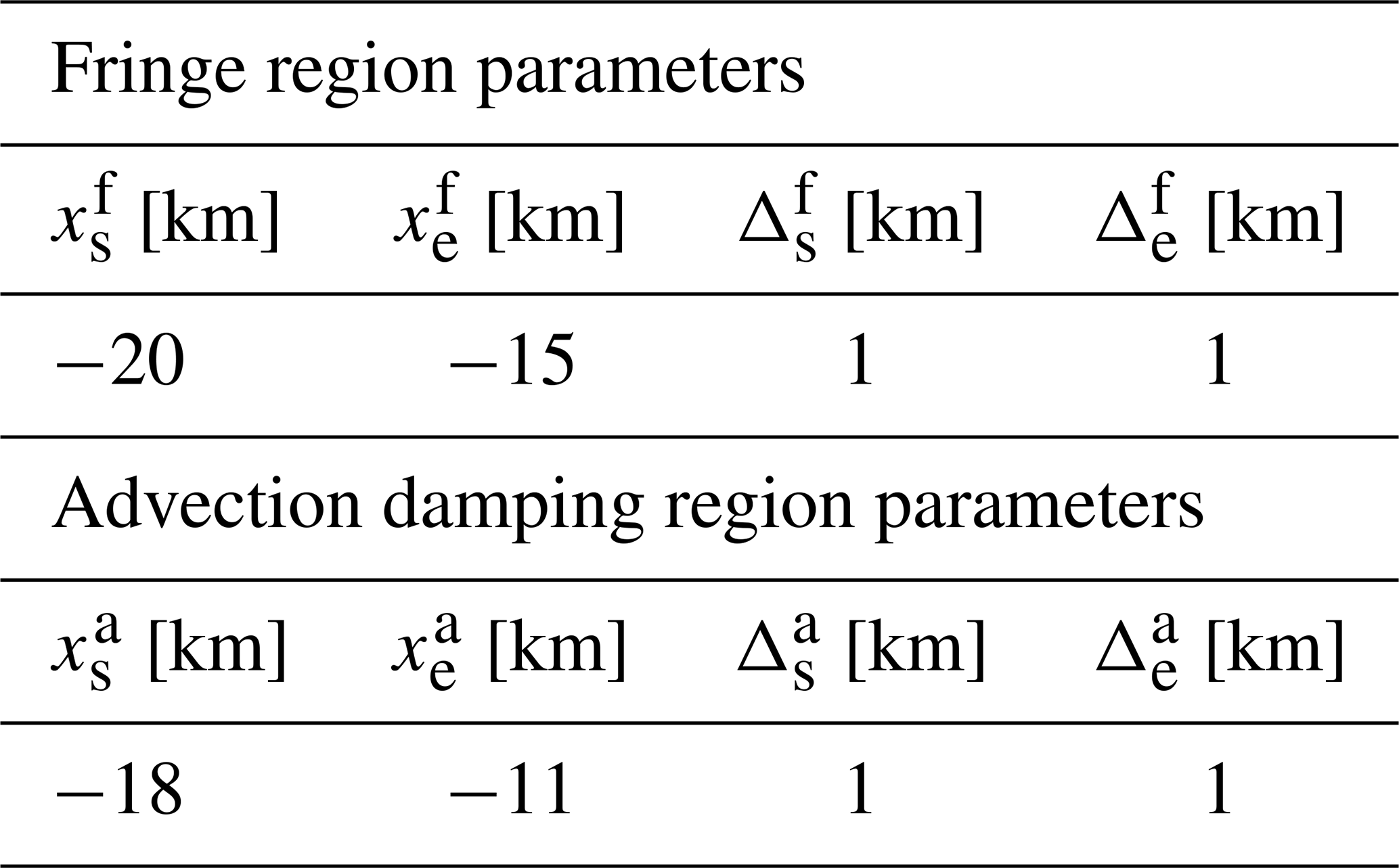
The parameters $x_{\mathrm{s}}^{\mathrm{f}}$ and $x_{\mathrm{e}}^{\mathrm{f}}$ are the start and end of the advection damping region, respectively, while ${\mathrm{\Delta }}_{\mathrm{s}}^{\mathrm{f}}$ and ${\mathrm{\Delta }}_{\mathrm{e}}^{\mathrm{f}}$ are the distances required to transition from zero to a damping equal to α_f and from α_f back to zero at the fringe start and exit, respectively. The parameter α_f is the fringe coefficient, which has to be tuned depending on the specific case. For instance, the potential temperature should also be damped according to Eq. 3, where u_i(x,t) and ${\stackrel{\mathrm{‾}}{u}}_i(\mathit{x},t)$ are replaced with θ(x,t) and $\stackrel{\mathrm{‾}}{\mathit{\theta }}(\mathit{x},t)$, respectively.

The unperturbed state required to compute the momentum and potential-temperature source terms in the fringe region is evaluated by conducting a second simulation – referred to as the concurrent precursor – without wind turbines, in a domain coincident to or larger than the fringe region. This has to advance simultaneously with the wind farm simulation, so that the unperturbed state is available at each iteration. The need to solve for a concurrent precursor and the higher cell count due to the inclusion of damping regions represent the main reasons for the increase in computational cost for the AGW-resolved method. Notably, streamwise periodic boundary conditions in the wind turbine domain allow the use of a single fringe region located at the inlet (Stipa et al., 2024a, present) or at the outlet (Lanzilao and Meyers, 2024).

An additional source of contamination of the physical solution is represented by spurious gravity waves that are generated by the fringe region as it tries to force the wave perturbations to zero. This issue has been addressed by Lanzilao and Meyers (2023), who developed the so-called advection damping region, where horizontal advection of the vertical velocity is brought to zero to prevent these spurious oscillations from being advected downstream. Specifically, the term $\partial \left(uw\right)/\partial x$ is multiplied by

$$\begin{array}{}\text{(6)}& {\mathit{\nu }}_{\mathrm{a}}(x,z)=\mathrm{1}-\left[F\left({\displaystyle \frac{x-x_{\mathrm{s}}^{\mathrm{a}}}{{\mathrm{\Delta }}_{\mathrm{s}}^{\mathrm{a}}}}\right)-F\left({\displaystyle \frac{x-x_{\mathrm{e}}^{\mathrm{a}}}{{\mathrm{\Delta }}_{\mathrm{e}}^{\mathrm{a}}}}+\mathrm{1}\right)\right]\mathcal{H}(z-H),\end{array}$$

where $x_{\mathrm{s}}^{\mathrm{a}}$ and $x_{\mathrm{e}}^{\mathrm{a}}$ are the start and end of the advection damping region, respectively, while ${\mathrm{\Delta }}_{\mathrm{s}}^{\mathrm{a}}$ and ${\mathrm{\Delta }}_{\mathrm{e}}^{\mathrm{a}}$ are the distances required to transition from unity to null magnitude of the advection term and from null back to unity at the region start and exit, respectively. ℋ(z−H) is the Heaviside function which ensures that this operation is only performed above the boundary layer in order to leave turbulence unaffected.

In the present paper, the hybrid off-line–concurrent method described in Stipa et al. (2024a) is used. This essentially reduces the computational cost associated with turbulence initialization in the concurrent precursor domain. In fact, while the size of the concurrent precursor has to be equal to or larger than the fringe region, the latter is required to compute the source terms only when the wind turbine simulation is started. Hence, turbulence spin-up can be achieved by first running a separate precursor in a reduced domain, referred to as the off-line precursor. In particular, since no gravity waves are expected during this phase, the vertical domain size is such that only a small portion of the free atmosphere is resolved. Moreover, if the ratio between the spanwise sizes of the concurrent and offline precursors is an integer, off-line precursor data can be prescribed at the inlet of the concurrent precursor by tiling them in the spanwise direction and extrapolating in the vertical. The concurrent precursor is then evolved using inlet–outlet boundary conditions for one flow-turnover time, i.e., until it is filled with this pre-calculated turbulent flow. Boundary conditions in the concurrent precursor are then switched to periodic, and the simulation becomes self-sustained. The hybrid off-line–concurrent precursor method allows the realization of a fully developed ABL within a domain that is sufficient to decorrelate turbulent fluctuations but whose size is not dictated by the wind-farm and AGW scales, thus allowing computational resources to be saved (see Stipa et al., 2024a for more details). In Fig. 1, a methodological sketch of the AGW-resolved approach employing the concurrent precursor method is displayed.

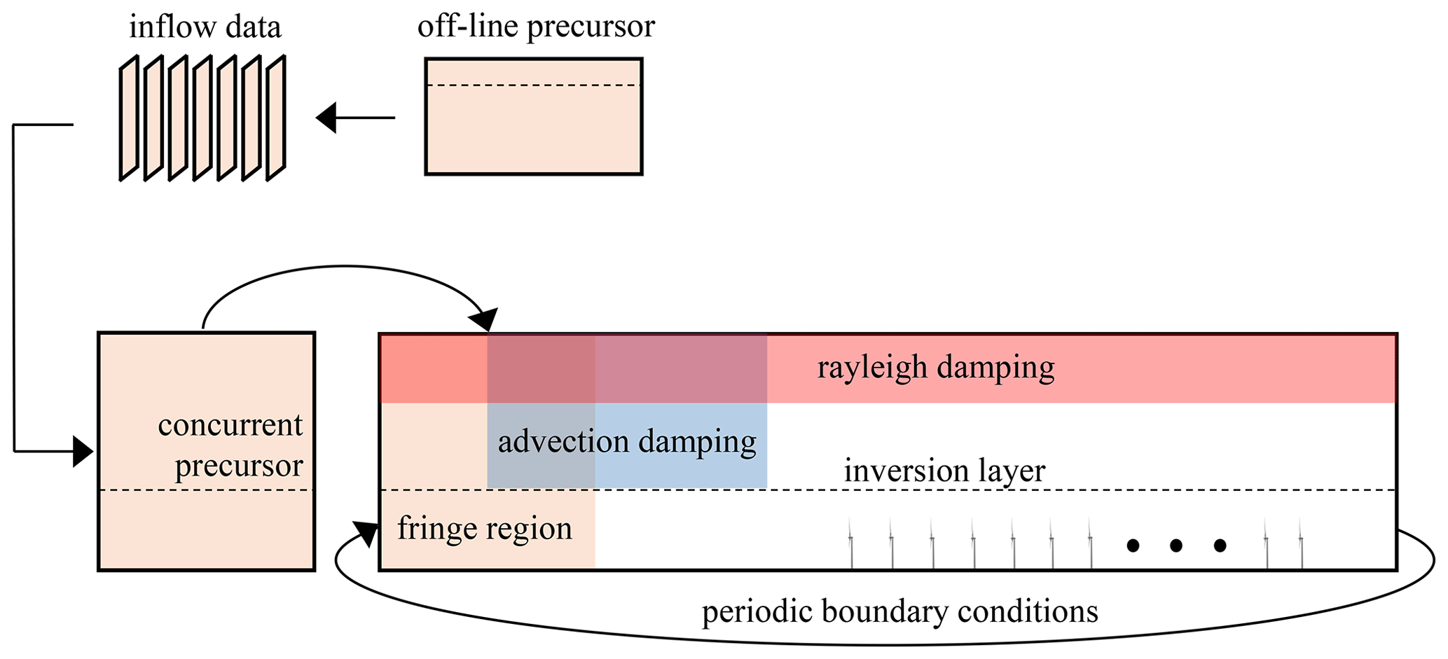
Figure 1 Methodological sketch of the AGW-resolved method employing streamwise periodic boundary conditions in the successor domain and a fringe region located at the inlet. The relative locations of the Rayleigh damping layer and advection damping region are also shown. The figure is not to scale.

2.2 AGW-modeled approach

As pointed out by Allaerts and Meyers (2017, 2018, 2019) and Lanzilao and Meyers (2022), AGWs in the free atmosphere induce large-scale pressure gradients inside the ABL. The MSC model developed by Stipa et al. (2024b) is based on the concept that the effect of AGW on the wind farm is given by the change in mean velocity produced by this horizontally heterogeneous pressure field, referred to here as p^*. Unfortunately, this idea cannot be directly applied to wind farm LES by prescribing p^* as a separate source term. In fact, for reasons that will be clarified later, the presence of the upper boundary automatically prescribes a certain horizontal pressure gradient inside the ABL such that mass and momentum conservation are satisfied. Specifically, we show below that the vertical streamline displacement η prescribed by the presence of the top boundary and the large-scale pressure field p^* cannot be imposed simultaneously; they are rather interdependent.

The relationship between these two variables can be explained by constructing a simple model based on a perturbation analysis applied to the depth-averaged linearized Navier–Stokes equations. Although this leads to a consistent simplification of the equations proposed by Allaerts and Meyers (2019) and cannot provide an accurate description of the boundary layer flow, this simple model still provides a level of physical insight that is sufficient to elucidate the relationship between the boundary layer displacement η and the pressure p^*. First, an infinitely wide wind farm is assumed in the spanwise direction, such that quantities can only change along the streamwise direction (i.e., $\partial /\partial y=\mathrm{0}$). Furthermore, the background flow is assumed to have a null mean spanwise component (i.e., Coriolis force is neglected). The structure of the potential temperature profile is that of a CNBL characterized by a lapse rate γ, an inversion strength Δθ, and an inversion height H. The bulk velocity within the boundary layer and the geostrophic wind are referred to as U and G, respectively. Similarly to Allaerts and Meyers (2019), the region below H is divided into two layers, namely the wind farm layer, characterized by a height H₁, and the upper layer of depth H−H₁. The depth of the wind farm layer is chosen to be twice the hub height, i.e., H₁=2h_hub. Finally, it is assumed that the wind farm and upper layer are characterized by the same background velocity U but, at the same time, admit different perturbation velocities u₁ and u₂. With the above simplifications, the 3LM equations derived by Allaerts and Meyers (2019) become

$$\begin{array}{}\text{(7)}& \left\{\begin{array}{l}U\frac{\partial u_{\mathrm{1}}}{\partial x}+\frac{\mathrm{1}}{\mathit{\rho }}\frac{\partial p^{*}}{\partial x}=-\frac{C}{H_{\mathrm{1}}}{u}_{\mathrm{1}}-\frac{f_x}{H_{\mathrm{1}}}\\ U\frac{\partial {\mathit{\eta }}_{\mathrm{1}}}{\partial x}+H_{\mathrm{1}}\frac{\partial u_{\mathrm{1}}}{\partial x}=\mathrm{0}\end{array}\right.\end{array}$$

for the wind farm layer and

$$\begin{array}{}\text{(8)}& \left\{\begin{array}{l}U\frac{\partial u_{\mathrm{2}}}{\partial x}+\frac{\mathrm{1}}{\mathit{\rho }}\frac{\partial p^{*}}{\partial x}=\mathrm{0}\\ U\frac{\partial {\mathit{\eta }}_{\mathrm{2}}}{\partial x}+H_{\mathrm{2}}\frac{\partial u_{\mathrm{2}}}{\partial x}=\mathrm{0}\end{array}\right.\end{array}$$

for the upper layer, where $C=\mathrm{2}{u}^{*\mathrm{2}}/U$. It should be noted that ${\mathit{\eta }}_{\mathrm{1}}+{\mathit{\eta }}_{\mathrm{2}}=\mathit{\eta }$, i.e., the total vertical displacement of the pliant surface initially located at H. This, at steady state, coincides with the flow streamline through H far upstream and can be thought of as the vertical displacement of the inversion layer or ABL.

Rewriting the system in terms of η leads to

$$\begin{array}{}\text{(9)}& \left\{\begin{array}{l}U\frac{\partial u_{\mathrm{1}}}{\partial x}+\frac{\mathrm{1}}{\mathit{\rho }}\frac{\partial p^{*}}{\partial x}=-\frac{C}{H_{\mathrm{1}}}{u}_{\mathrm{1}}-\frac{f_x}{H_{\mathrm{1}}}\\ U\frac{\partial u_{\mathrm{2}}}{\partial x}+\frac{\mathrm{1}}{\mathit{\rho }}\frac{\partial p^{*}}{\partial x}=\mathrm{0}\\ U\frac{\partial \mathit{\eta }}{\partial x}+H_{\mathrm{1}}\frac{\partial u_{\mathrm{1}}}{\partial x}+H_{\mathrm{2}}\frac{\partial u_{\mathrm{2}}}{\partial x}=\mathrm{0}.\end{array}\right.\end{array}$$

To complete the system, an extra equation is added that relates the vertical inversion displacement to the pressure anomaly felt inside the boundary layer due to the increase or decrease in weight of the air column overtopping a given x. This can be expressed in Fourier space by means of linear theory (Nappo, 2012; Lin, 2007) as

$$\begin{array}{}\text{(10)}& {\displaystyle \frac{\mathrm{1}}{\mathit{\rho }}}{\widehat{p}}^{*}=\mathrm{\Phi }\widehat{\mathit{\eta }},\end{array}$$

where the hat denotes Fourier coefficients and Φ is the so-called complex stratification coefficient, which accounts for pressure anomalies generated by both the inversion layer displacement (surface waves) and the resulting perturbations aloft (internal waves). We refer to Smith (2010) for the definition of this function; in this context, it is sufficient to notice that all the physics related to AGWs and thermal stratification enters the system through the complex stratification coefficient Φ, while Eq. (9) does not contain any stability-related term.

Equations (9) and (10) form a fully determined system which can be easily solved upon transforming Eq. (9) into Fourier space. In particular, Eq. (9) describes the flow physics below H, while Eq. (10) refers to the flow in the free atmosphere. It can be observed that the pressure field p^*, which satisfies both Eqs. (9) and (10), is the one that reconciles momentum and mass conservation inside the boundary layer with the pressure anomalies due to overtopping density differences produced by a determined vertical displacement of the pliant surface at H. Specifically, η represents the coupling variable between the ABL and the free atmosphere, i.e., the neutral and stratified regions of the flow, respectively, under CNBL. Now, focusing only on the flow below H, i.e., on Eq. (9), it is evident that the pressure gradient induced by AGWs – and its effects on the velocity – can be readily obtained without any knowledge about the free atmosphere stratification if the correct inversion displacement η is somehow known a priori. The same reasoning can be applied to the full 3LM equations derived by Allaerts and Meyers (2019) for the first two layers by simply noticing that the number of unknowns is reduced by 1. Extending this idea to LES, the knowledge of η can be used to vertically deform the top boundary of the computational domain when it is initially located at H. Since a slip condition is usually applied here, deforming the upper boundary alters the mean flow streamlines in a manner that is consistent with the inversion layer displacement, allowing the mean AGW-induced pressure gradient to be automatically recovered within the ABL. In summary, the effects of AGWs produced by different stability conditions can be easily modeled by using their corresponding η field to vertically deform the upper boundary. By doing so, the LES can be confined to the turbulent part of the flow capped below the start of the stable-flow region, where the wind farm is located.

In the present study, the top boundary is placed at the inversion center and the MSC model is used to compute η. The vertical displacement is linearly distributed to the underlying mesh points, deforming the computational grid before the simulation is started. This means that, at each horizontal location, the mesh point located at the wall is not displaced, while the furthest is moved vertically by η. The grid points in between will be displaced from zero to η, depending on their distance from the wall, thus causing vertical cell stretching.

The case where the top boundary is a flat surface corresponds to the rigid-lid limiting solution. In particular, while this differs from the actual solution with atmospheric gravity waves, it still models – to a certain extent – both the global blockage and the flow acceleration within the wind farm produced by flow confinement inside the boundary layer. We highlight that flow confinement and free-atmosphere stability effects are different ways to refer to the same physical manifestation. In fact, in light of the unique relationship between pressure and ABL displacement, stability effects determine an inversion displacement such that the pressure perturbations induced by flow confinement and by AGWs are equivalent; i.e., they satisfy both Eqs. (9) and (10). For this reason, the rigid-lid assumption models global blockage to a certain degree, as the flow is indeed confined. However, the mechanism under which such confinement happens disregards gravity waves by neglecting the inversion perturbation field that complies with the actual potential temperature structure.

As a further consideration for the AGW-modeled technique, since the overall pressure disturbance is fully determined by the inversion displacement, any spatially varying source term imposed in the form of a pressure gradient will not produce any effect on the simulation results but will instead change the significance of the pressure variable such that the overall pressure disturbance that complies with the imposed streamline displacement is retained.

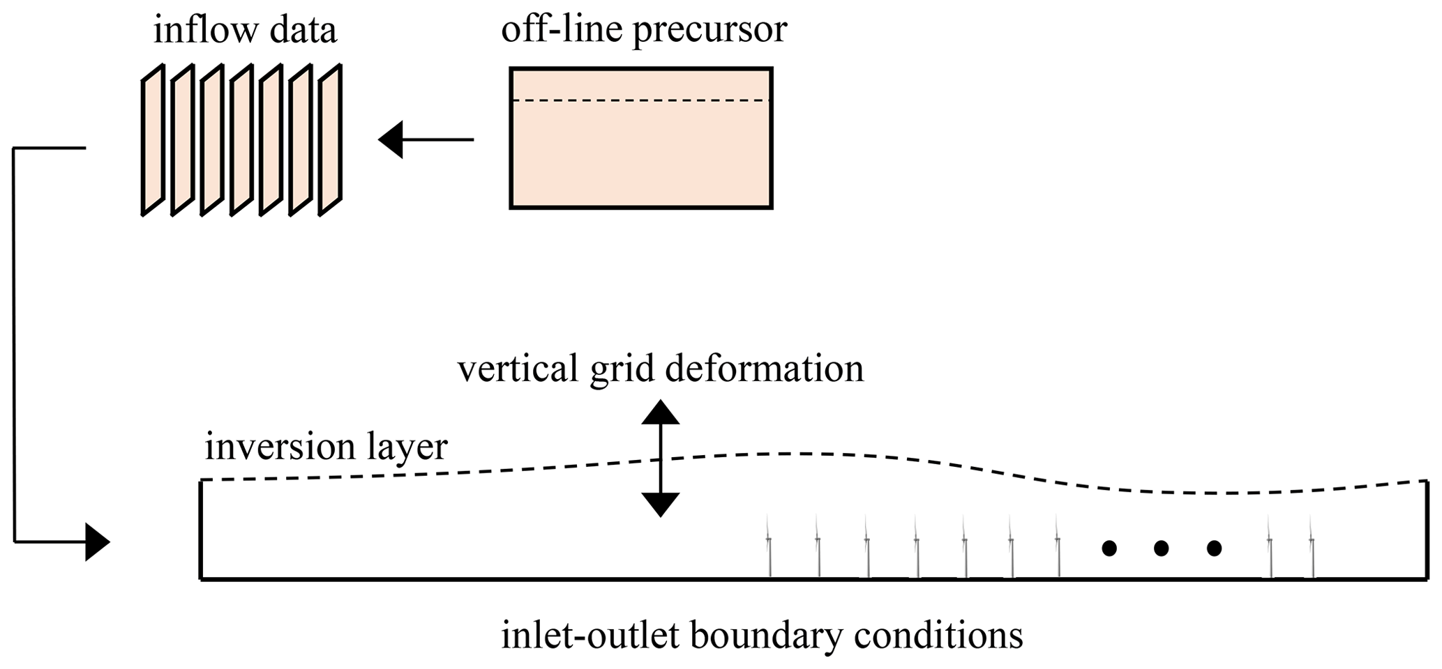
The developed approach, sketched in Fig. 2, is convenient for at least three reasons. First, it substantially reduces the computational cost by eliminating the need for damping regions and the requirement for a domain that is large enough to vertically resolve AGWs. Secondly, it does not require a concurrent precursor to be run simultaneously to the wind farm simulation. Third, under CNBLs, it eliminates the need to solve for a potential-temperature transport equation, as the flow below H is neutral. This condition is only violated very close to the top boundary, where discrepancies in turbulent fluctuations produced by the absence of stability and by the physical boundary are deemed acceptable, as they happen away from the wind farm. Moreover, at the inversion height, fluctuations are naturally close to zero, as this roughly coincides with the top of the boundary layer.

Figure 2 Methodological sketch of the AGW-modeled method. The figure is not to scale.

A limitation of the proposed method is that the accuracy of the large-scale pressure gradient produced by displacing the top boundary is dependent on the accuracy of the MSC model in predicting the overall AGW physics. Stipa et al. (2024b) showed that the pressure disturbance produced by the MSC model agrees well with AGW-resolved wind farm LES simulations for different values of capping inversion strength. Another limitation is given by the fact that the MSC model has not been tested for values of $H/H_{\mathrm{1}}$ that are less than or equal to 1, a realistic condition for modern large turbines. This corresponds to a situation where the turbine top tip almost pierces the inversion layer, with the consequent disappearance of the upper layer. Devesse et al. (2023) developed an alternative strategy to the one used in the MSC model to couple the 3LM of Allaerts and Meyers (2019) and the wake model of Bastankhah and Porté-Agel (2014), which also uses the 3LM to address AGW effects. When validating this new model against wind farm LESs characterized by $H=\mathrm{150},\mathrm{300},\mathrm{500}$ and 1000 m and h_hub=119 (Lanzilao and Meyers, 2024), the authors excluded LES cases with $H/H_{\mathrm{1}}=\mathrm{0.63}$ (H=150 m). Among the remaining cases, the model showed the highest deviation from the LES when $H/H_{\mathrm{1}}=\mathrm{1.26}$ (H=300 m). As the MSC model also uses the 3LM to model AGW effects, these results suggest that the MSC model will lose accuracy when $H/H_{\mathrm{1}}\lesssim \mathrm{1.5}$. In the present manuscript, the dependency of the proposed technique on the ratio $H/H_{\mathrm{1}}$ is not investigated, and this number is fixed at 2.78. Although this is a limitation of the MSC model, if η could be evaluated by a different means (e.g., with a coarser AGW-resolved LES employing a simple canopy model) at a height located above the inversion layer, the AGW modeling approach could be used for small $H/H_{\mathrm{1}}$ ratios by placing the upper boundary a few hundred meters into the free atmosphere and by including the potential-temperature transport equation. A related limitation applies to those cases characterized by an unsteady flow in the free atmosphere, as the MSC model assumes steady-state conditions.

3 Suite of simulations

To verify the validity of the proposed approach, we use the two LES simulations available from Stipa et al. (2024b). These correspond to a subcritical and a supercritical regime of interface waves within the inversion layer and are characterized by damping regions and a domain size that is sufficient to resolve AGWs in the free atmosphere. For this reason, they are referred to as “AGW-resolved” cases in the present study. Each case is then compared to its AGW-modeled counterpart, where the technique proposed in Sect. 2.2 is applied. Once validated, the AGW-modeled approach is leveraged to simulate a case corresponding to the rigid-lid limiting solution, where the top boundary is not associated with any vertical displacement. This analysis is motivated by the fact that the rigid lid enforces a dependency on the inversion layer height while discarding the full AGW solution, making it an appealing approximation in the context of reduced-order engineering parametrizations. As will be shown, its estimates for the blockage are, in some cases, better than those of a conventional wake model combined with a local induction model, which only account for local turbine induction.

3.1 AGW-resolved simulations

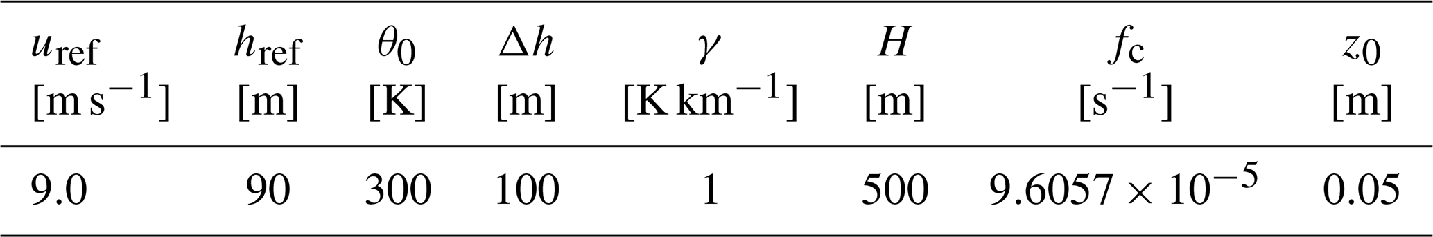
The subcritical and supercritical regimes of the AGW-resolved CNBL simulations are obtained by setting the inversion strength to 7.312 and 4.895 K, respectively. Table 1 summarizes the remaining input parameters, namely the reference velocity u_ref at the reference height h_ref (chosen as the hub height), the reference potential temperature θ₀, the lapse rate γ, the inversion height H, and the equivalent roughness length z₀. The Coriolis parameter f_c corresponds to a latitude of 41.33° N. The simulated wind farm has a rectangular planform, with 20 rows and 5 columns organized in an aligned layout. The first row is located at x=0 and extends from 300 to 2700 m in the spanwise direction. This determines a lateral spacing of 600 m (4.76 D), while the streamwise spacing is set to 630 m (5 D). Wind turbines are assumed to be NREL 5 MW reference turbines and are equipped with the angular velocity and pitch controllers described in Jonkman et al. (2009). A very simple yaw controller is also added, which rotates the wind turbines independently at a constant rotation speed of 0.5° s⁻¹ when the flow misalignment exceeds 1°. The flow angle for the yaw controller is calculated by filtering the wind velocity at a sampling point located 1 D upstream of the rotor center using a time constant of 600 s. Turbines are modeled using the actuator disk model (ADM) described in Stipa et al. (2024a), while the tower and nacelle are not included in the simulation. The ADM force projection width is set to 18.75 m.

Table 1 Reference velocity u_ref at the reference height h_ref, reference potential temperature θ₀, inversion width Δh, lapse rate γ, inversion center H, Coriolis parameter f_c, and equivalent roughness height z₀, which were used as input for the finite wind farm simulations presented in this section.

The AGW-resolved simulations employ the hybrid off-line–concurrent precursor method described in Stipa et al. (2024a). For the off-line precursors, the Rampanelli and Zardi (2004) model is used to initialize the potential-temperature profile, where H is taken as the center of the capping inversion layer. Off-line precursors for both ABL conditions are advanced in time for 10⁵ s, after which the data are averaged for 2×10⁴ s. Results from this phase are reported in Appendix A. The off-line precursor domain size is of 6 km × 3 km × 1 km in the streamwise, spanwise, and vertical directions, respectively. The mesh has a horizontal resolution of 15 m, while in the vertical direction, it is graded the same as in the concurrent-precursor and successor simulations described later. A driving pressure controller that employs the geostrophic-damping method is used to fix the average velocity at h_ref while eliminating inertial oscillations in the free atmosphere. Moreover, a potential-temperature controller is used to fix the average potential temperature profile throughout the simulation (both controllers and the geostrophic damping use the settings reported in Stipa et al., 2024a). Inflow slices saved during the off-line-precursor phase are then used to feed the concurrent precursor for one flow through time (approximately 700 s). Then, boundary conditions in the concurrent-precursor domain are switched to periodic and the solution becomes self-sustained. At each successor iteration, the velocity and temperature from the concurrent precursor are used to compute the damping terms for the momentum and temperature equations inside the fringe region located at the inlet of the successor domain. This allows a time-varying turbulent flow to be produced at the fringe exit while eliminating the reintroduction of the wind farm wake at the inlet by the periodic boundaries. Moreover, the fringe region allows gravity wave reflections to be damped. At the upper boundary, a Rayleigh damping layer is used with a thickness of 12 km, i.e., slightly more than one expected vertical wavelength λ_z (this parameter can be estimated as explained in Sect. 1). Lateral boundaries are periodic, implying that gravity waves induced by the wind farm will interact with their periodic images. This dictates that the domain must be sufficiently large for these interactions to happen far from the wind turbines. The advection damping technique described in Sect. 2.1 is used to ensure that interactions between fringe-generated and physical gravity waves are not advected downstream but instead remain trapped inside the advection damping region. The Rayleigh damping coefficient α_r is set to 0.05 s⁻¹, while the fringe damping coefficient α_f is set to 0.03 s⁻¹. The fringe- and advection-damping functions are given by Eqs. (4) and (6), respectively, and their parameters are reported in Table 2.

Table 2 Fringe- and advection-damping region parameters.

The domain size of the AGW-resolved successor cases is 40 km × 21 km × 28 km in the streamwise, spanwise, and vertical directions, respectively, and it is discretized with 1554 × 1194 × 345 cells. All directions are graded to reach a mesh resolution of 30 m × 12.5 m × 10 m around the wind farm, as reported by Stipa et al. (2024b). The concurrent-precursor mesh coincides with the portion of the successor domain located inside the fringe region. As a consequence, it extends for 5 km × 21 km × 28 km. Here, the mesh resolution is identical to that of the successor mesh.

3.2 AGW-modeled simulations

The AGW-modeled simulations feature the same horizontal domain size and discretization as the AGW-resolved cases. Conversely, the vertical domain size is set to 500 m, which is coincident with the unperturbed inversion layer height. Since the fringe region and the Rayleigh- and advection-damping layers are not required, inlet–outlet boundary conditions are used in the streamwise direction. Due to the fact that the inflow data used in the AGW-resolved cases are not available because they are generated at run time within the concurrent precursor, two additional off-line precursor simulations corresponding to the subcritical and supercritical conditions defined in Sect. 3.1 are conducted. These are first run for 10⁵ s, after which data are averaged for 4×10⁴ s and inflow sections are saved at each iteration to be used as inlet boundary conditions in the wind farm successors. These additional precursor cases are characterized by an enlarged spanwise domain size of 21 km – coincident with the successor cases – to avoid the spanwise periodization of the inflow data that characterizes the initial condition for the AGW-resolved cases in Stipa et al. (2024b). As reported by the same authors, this led to turbulent streaks that slowed down the convergence of turbulence statistics. To further address this issue, a spanwise shift velocity of 1 m s⁻¹ is applied to the inflow data in the AGW-modeled successor simulations, with the objective of enhancing the convergence of statistics. Instead of being added to the inflow velocity field, this shift velocity is used to physically move the inflow data along the spanwise direction so that the average wind direction remains unaffected. Results from these off-line precursors characterized by an enlarged domain are reported in Appendix A, together with their comparison with the off-line precursors conducted for the AGW-resolved simulations. The inflow data are then mapped at the successor inlet patch by means of bilinear interpolation, further interpolating at the desired time value from the two closest available times. AGW-modeled simulations are progressed in time for 4×10⁴ s using the entire inflow database. This differs from the AGW-resolved cases, which are only progressed for 2×10⁴ s. Since the unperturbed flow corresponds to a CNBL, we do not solve for potential temperature, as this is constant throughout the simulation domain. As explained in Sect. 2.2, stability effects on the ABL flow are embedded in the applied vertical displacement of the inversion layer, which imposes the corresponding pressure perturbation. As previously mentioned, this is calculated using the MSC model. The input parameters for the MSC model are calculated using the fully developed off-line precursors of the AGW-resolved cases to ensure consistency between these and the AGW-modeled simulations. Although the input parameters required by the MSC model are detailed in Stipa et al. (2024b), they are also reported in Table 3 for completeness. The resulting inversion displacement fields are displayed in Fig. 3. For more details about the MSC model setup, the reader is referred to Stipa et al. (2024b), where the same atmospheric conditions are investigated.

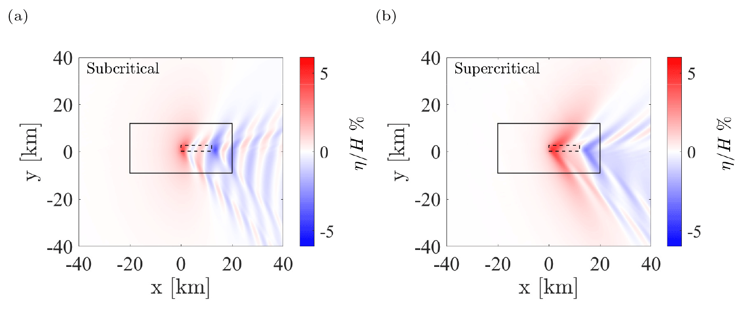
Figure 3 Inversion displacement as a percentage of the boundary layer height for (a) the subcritical case and (b) the supercritical case. The LES domain is identified by the continuous rectangle, while the wind farm is represented by the dashed rectangle.

Table 3 MSC model input parameters for the subcritical and supercritical cases. The parameters ν_t,1 and ν_t,2 are the deep-averaged effective viscosities in the wind-farm and upper layers, evaluated using the Nieuwstadt (1983) model; U_i and V_i (with $i=\mathrm{1}:\mathrm{3}$) are, respectively, the streamwise and spanwise velocity components, deep averaged from the AGW-resolved off-line precursors within layer i; TI_∞ is the hub-height freestream turbulence intensity. Rows with a single value imply that the value applies to both cases.

Regarding the simulation corresponding to the rigid-lid approximation, the velocity inflow data from the subcritical case are used to prescribe the inlet boundary condition, while the top boundary, also located at H=500 m, is not displaced.

4 Results

In the following, the accuracy of the proposed AGW-modeled method is first verified against AGW-resolved simulations corresponding to Stipa et al. (2024b) for both subcritical and supercritical conditions in Sect. 4.1. Then, in Sect. 4.2, the implications of employing the rigid-lid approximation (Smith, 2024) in terms of our ability to capture global blockage effects are investigated. The latter corresponds to an infinitely high free-atmosphere stability obtained by modeling the inversion layer as a rigid lid. As a consequence, the resulting horizontal pressure gradient solely responds to the requirement for mass conservation inside the boundary layer.

For the cases presented in this manuscript, the AGW-modeled technique requires a domain with ≈12.7 % of the grid cells used for the AGW-resolved simulations. Although the domain used for the off-line precursors is larger for the AGW-modeled cases, this is not a requirement of the developed approach. In fact, a smaller domain with the lateral inflow periodization technique is probably sufficient if combined with the spanwise shift used in this article to accelerate the convergence of statistics.

The AGW-resolved and AGW-modeled cases consist of 15 000 and 35 000 s of available data, respectively, following the establishment of a statistically steady flow in the successor simulations. However, when comparing turbine quantities, time averaging was performed for 15 000 s in both cases. Specifically, since the AGW-modeled cases used different precursor time histories from their AGW-resolved counterparts, the start of the time-averaging window was shifted in time until the row-averaged freestream velocity at the first turbine row matched those from the corresponding AGW-resolved simulations. This allowed us to compare the two approaches while eliminating any bias in freestream wind speed produced by the different large-scale turbulent structures in the two cases. More details on this procedure and the motivation for using it are reported in Appendix B. This approach was only followed when comparing turbine power and thrust between the AGW-resolved and AGW-modeled simulations. Elsewhere, results were always averaged across the entirety of the available time history.

4.1 Model verification

While the local blockage is given by the combination of individual turbine induction effects, global blockage can be explained as the flow response to the pressure gradient induced by the mean ABL displacement (Stipa et al., 2024b). In turn, this results from the vertical velocity perturbation produced by the wind farm and the corrective response provided by buoyancy forces. The induced perturbation pressure field is heterogeneous in space and features an unfavorable pressure gradient region upstream of the farm and a favorable region that extends throughout most of the cluster. Downstream and around the wind farm, the perturbation pressure field is strongly dependent on the strength of the inversion, the free-atmosphere lapse rate, and the geostrophic wind.

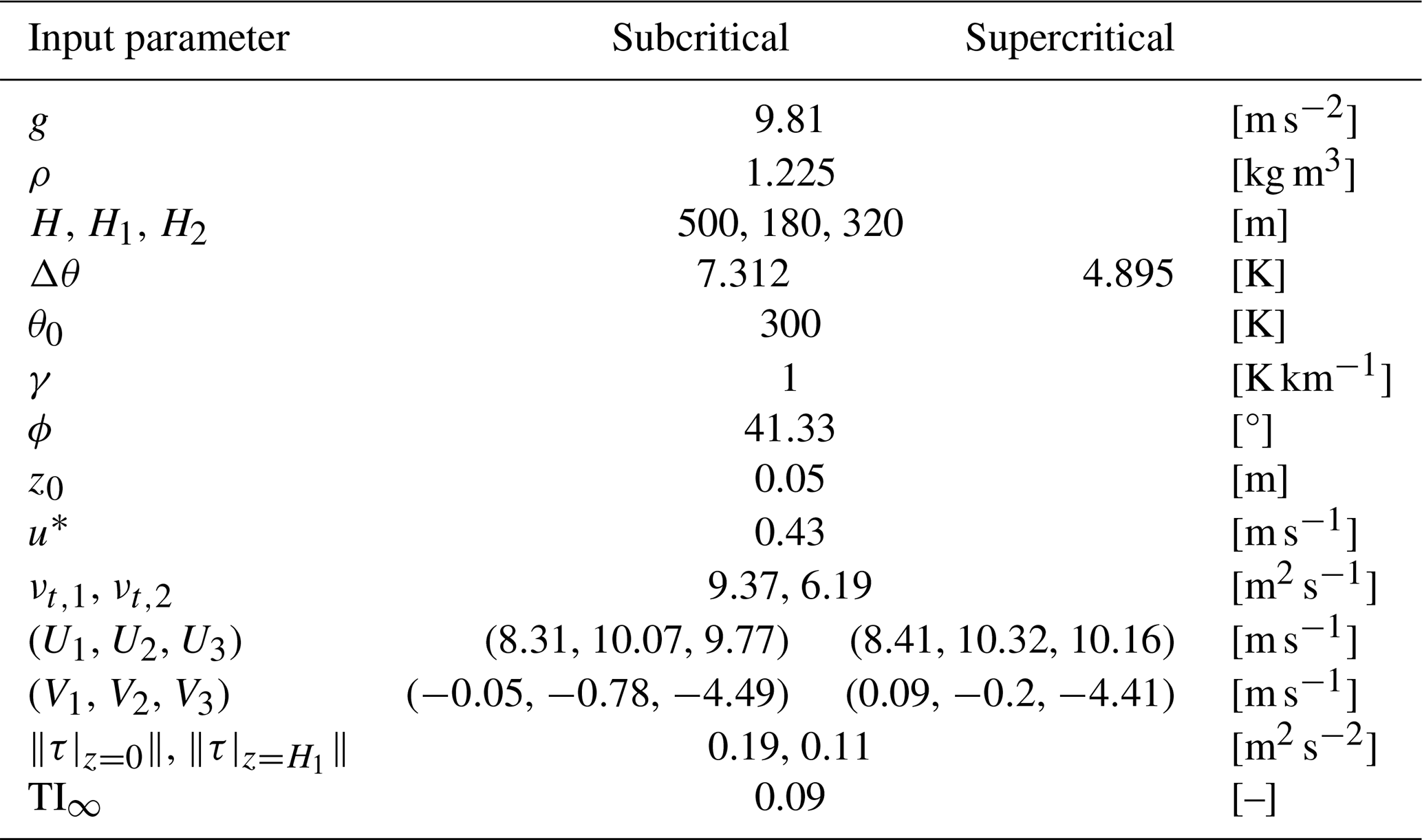
In light of the critical role played by the perturbation pressure field, we first compare the mean pressure variations resulting from the AGW-modeled approach with those obtained by resolving gravity waves in the free atmosphere. Figure 4 plots the streamwise distribution of the pressure perturbation averaged over the wind farm width and in the upper layer (from H₁ to H) for both the subcritical and supercritical cases, as obtained using the AGW-resolved and AGW-modeled approaches. For completeness, the pressure variation resulting from the MSC model is also reported. In both atmospheric states, all models predict similar trends in the pressure perturbation distribution. As explained in Sect. 2.2, the latter is a function of the imposed vertical boundary layer displacement for the AGW-modeled simulations, while it naturally arises from the free-atmosphere solution in both the AGW-resolved approach and the MSC model. Subcritical conditions produce larger pressure gradients if compared to the supercritical ABL state; these are unfavorable upstream and favorable inside the wind farm. Moreover, in subcritical conditions, lee waves (visible in Fig. 3) induce pressure oscillations with a wavelength that is lower than the wind farm length. As can be appreciated from Fig. 4, these oscillations are superimposed on the favorable pressure gradient inside the wind farm and lead to oscillations in the background velocity field, power variations throughout the wind farm, and intermittent wake recovery downstream.

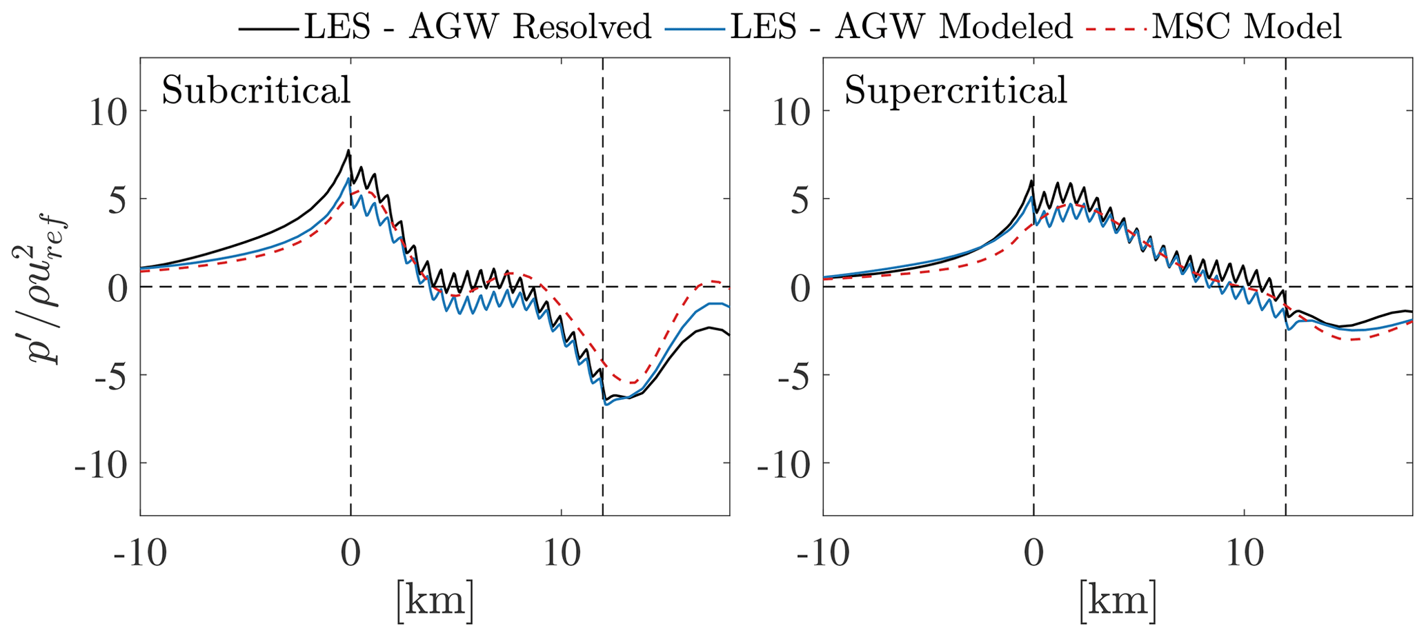
Figure 4 Time-averaged streamwise distribution of the pressure perturbation, further averaged over the wind farm width (between y=0 and y=3000 m) and the upper layer (from H₁ to H), for both the subcritical and supercritical cases. For completeness, the pressure variation resulting from the MSC model is also shown as a dashed red line. The AGW-resolved and AGW-modeled results are shown in black and blue, respectively.

The differences between the pressure disturbances predicted by the AGW-resolved, AGW-modeled, and MSC results can be explained as follows. First, with reference to the AGW-modeled and MSC model results, differences in the pressure disturbance are attributable to the simplifications made in the MSC model, such as linearity, the simpler parametrization of the wind farm and of the turbulent momentum fluxes, and the lack of resolved turbulence. As a consequence, even though η is identical in the two approaches, these aspects inevitably affect the momentum budget, leading to differences in both velocity and pressure. Regarding the AGW-resolved and AGW-modeled approaches, differences in the pressure field arise from differences between the imposed η distribution (AGW-modeled approach) and the η distribution that develops naturally (AGW-resolved approach), although the two methods share the same accuracy inside the ABL. Notably, both the MSC and AGW-modeled approaches are able to capture the different trends in pressure disturbance arising from the potential-temperature structure in the subcritical and supercritical cases. This is achieved at a drastically lower computational cost than with the AGW-resolved method, in our opinion justifying the pressure deviations observed in Fig. 4, which are bounded by a maximum value of $\mathrm{1.5}\mathit{\rho }{u}_{\mathrm{ref}}^{\mathrm{2}}$. Moreover, the arguments provided in Sect. 2.2 regarding the role of the pressure variable are confirmed, as its dependence on free-atmosphere stability is captured in the AGW-modeled approach without solving for the potential-temperature equation. Finally, the mismatch in p^′ between the AGW-modeled and AGW-resolved results near the end of the domain in Fig. 4 is produced by the fringe region employed at the domain inlet in the AGW-resolved simulations. As explained in Sect. 2.2, the fringe region removes the wind farm wake by forcing the flow to adhere to the concurrent-precursor solution at the fringe exit. In doing so, it modifies the momentum balance, altering the pressure field both inside and immediately upwind of the fringe region, which coincides with the domain exit in Fig. 4 owing to the periodic boundary conditions.

Figure 5 shows the streamwise evolution of hub-height velocity averaged over time and over the wind farm width for both the subcritical and supercritical ABL states, based on the AGW-resolved and AGW-modeled methods. On the right panel, the metric $(u_{\mathrm{AGWM}}-u_{\mathrm{AGWR}})/u_{\mathrm{AGWR}}$ in percent is also reported, showing the relative percentage error of the velocity predicted by the AGW-modeled approach with respect to the AGW-resolved approach. Results from the two models are in excellent agreement with each other, indicating that the proposed methodology is able to capture not only the blockage but also the entirety of the gravity wave effects on the ABL flow. Velocity reductions extending several kilometers upstream of the wind farm can be observed in both cases, indicating the presence of global blockage. Moreover, the mean velocity deficit in the wind farm wake is captured equivalently using both methods; the effect of gravity-wave-induced pressure gradients on promoting wake recovery can be observed, especially for the subcritical case. Regarding the error in the velocity, the differences between the two approaches are approximately ±5 % inside the wind farm and −1 % outside, which is small enough that it becomes difficult to state if they are due to the AGW-modeled technique or attributable to the differences in the inflow data. Notably, this seems to be the case for supercritical conditions in the region upstream of the wind farm, where results from the AGW-resolved method depict a higher velocity than the AGW-modeled simulations.

Figure 5 Time-averaged hub-height velocity, further averaged over the wind farm width (between y=0 and y=3000 m), for subcritical (a) and supercritical (c) conditions, as obtained using both the AGW-resolved (black) and AGW-modeled (orange) approaches. In (b), the relative error of the AGW-modeled method with respect to the AGW-resolved method, defined as $(u_{\mathrm{AGWM}}-u_{\mathrm{AGWR}})/u_{\mathrm{AGWR}}$ (in percent), is shown.

Figure 6 Comparison of row-averaged thrust and power distributions for the subcritical (a) and supercritical (b) cases. Time averaging is performed as described in Appendix B. AGW-resolved data are shown in black, while results from the AGW-modeled simulations are depicted in blue.

Table 4 Overall wind farm power obtained from LES in subcritical and supercritical conditions using the AGW-resolved and AGW-modeled techniques. In addition, the total, non-local, and wake wind farm efficiencies η_tot, η_nnl, and η_w, respectively, are reported. The value of P_∞ required to compute η_nnl was obtained from the data reported in Appendix B of Stipa et al. (2024b).

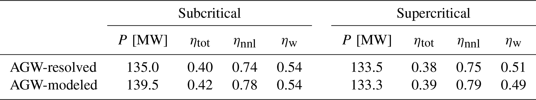
In order to verify the accuracy of the proposed method in capturing the turbine thrust and power trends along the wind farm length, the time- and row-averaged thrust and power at each wind farm row are plotted in Fig. 6 for both the subcritical and supercritical cases. In order to consistently average over time, the approach described in Appendix B was used. The effect of lee waves aloft in the subcritical case can be appreciated by looking at the large-scale oscillations in thrust and power throughout the wind farm. Moreover, the weaker favorable pressure gradient that characterizes supercritical conditions implies lower power towards the wind farm exit. Conversely, the subcritical state is affected by a stronger unfavorable pressure gradient upwind, leading to increased blockage effects. In general, increased blockage also leads to a stronger favorable pressure gradient within the wind farm. However, as demonstrated by Lanzilao and Meyers (2024), whether the net result is beneficial or detrimental depends on the specific conditions. Overall, it can be stated that the proposed AGW-modeled approach captures the effects of gravity waves on the wind farm power, which is arguably the most important information obtained from a wind farm LES. Table 4 reports the overall wind farm power as well as the non-local, wake, and total wind farm efficiencies η_nnl, η_w and η_tot, respectively, as defined by Lanzilao and Meyers (2024) as follows:

$$\begin{array}{}\text{(11)}& {\mathit{\eta }}_{\mathrm{nnl}}={\displaystyle \frac{P_{\mathrm{1}}}{P_{\mathrm{\infty }}}},{\mathit{\eta }}_{\mathrm{w}}={\displaystyle \frac{P_{\mathrm{tot}}}{N_{\mathrm{t}}{P}_{\mathrm{1}}}},{\mathit{\eta }}_{\mathrm{tot}}={\mathit{\eta }}_{\mathrm{nnl}}{\mathit{\eta }}_{\mathrm{w}},\end{array}$$

where P₁ is the average power at the first wind farm row, P_tot is the total wind farm power, N_t is the total number of wind turbines, and P_∞ is the power that an isolated wind turbine would experience in the same operating conditions. Notably, η_nnl quantifies blockage effects, η_w provides information on wake effects, while η_tot refers to the overall wind farm efficiency. In order to compute η_nnl, the power P_∞ produced by an isolated wind turbine subject to the same conditions is required. To get this information, Lanzilao and Meyers (2024) conducted an additional isolated turbine LES that employed the same inflow time history used in the wind farm simulations. In our case, the inflow data are not available for the AGW-resolved simulations, as they are generated at runtime and not saved to disk. Hence, we use the turbine data reported in Appendix B of Stipa et al. (2024b) to compute P_∞ by interpolating the turbine power curve using the hub-height freestream velocity experienced at the domain inlet of each simulation, averaged over the entirety of the available samples. Since the data from Stipa et al. (2024b) are evaluated from LESs characterized by uniform inflow and the absence of turbulence, the values of η_nnl and η_tot likely differ from the figures that would be obtained using the same inflow data as in the AGW-resolved and AGW-modeled simulations. However, the differences in each parameter between the two methodologies can still be compared, highlighting the ability of the proposed method to capture blockage and wake effects.

The obtained values of η_w agree better than those of η_nnl between the AGW-resolved and AGW-modeled cases for both subcritical and supercritical conditions. The AGW-modeled method captures both the increase in blockage effects from supercritical to subcritical conditions (η_nnl from 0.79 to 0.78) and the efficiency improvement resulting from the favorable pressure gradient throughout the wind farm in the subcritical case (η_w from 0.49 to 0.54). The fact that values of η_nnl differ more than those of η_w between the two methodologies suggests that the variations in total wind farm power – and consequently those in η_tot – are mostly due to a power bias at the first row rather than an inconsistency distributed over the entire wind farm. However, we believe that differences in the turbulent inflow data between the AGW-resolved and AGW-modeled simulations are the main cause of this power bias at the first row, considering the extremely good agreement in hub-height velocity observed in Fig. 5.

4.2 Implications of the rigid-lid approximation

In the present section, the proposed methodology is leveraged to assess the implications of the rigid-lid approximation when evaluating global blockage effects. The simpler formulation with respect to the full AGW solution renders the rigid-lid assumption attractive for potential use in future fast engineering models. However, neither its relation to the full AGW solution nor its differences when compared with a truly neutral case where stratification is absent have been assessed in detail yet.

To enforce the rigid-lid approximation within LES, we employ the AGW-modeled technique with no vertical displacement of the top boundary, which is located at 500 m. Figure 7 shows the mean streamwise distributions of hub-height velocity and depth-averaged pressure between H₁ and H averaged over the width of the wind farm, i.e., from y=0 m to y=3000 m. In particular, it compares the subcritical, supercritical, and rigid-lid cases obtained using the AGW-modeled approach. A close-up view of the blockage region within 1 km upstream of the wind farm is also reported. First, by looking at the pressure gradient, it can be noticed that each case is characterized by an anti-symmetric pressure distribution with the maximum and minimum at the wind farm start and exit, respectively. Moreover, the rigid-lid approximation is characterized by the presence of the lowest values of the favorable and unfavorable pressure gradients upstream and inside the wind farm, respectively. As a consequence, while the rigid-lid approximation features global blockage, this is less pronounced than under the subcritical or supercritical conditions. Regarding wake recovery, results from the rigid-lid case exhibit the highest deficit. Overall, while it is clear that the rigid-lid approximation differs from the full gravity wave solution in terms of pressure perturbations, wake recovery, and farm blockage, our results suggest that flow confinement associated with a homogeneous – instead of heterogeneous – inversion height may be responsible for the majority of the global blockage effects. This concept will be expanded further in this section.

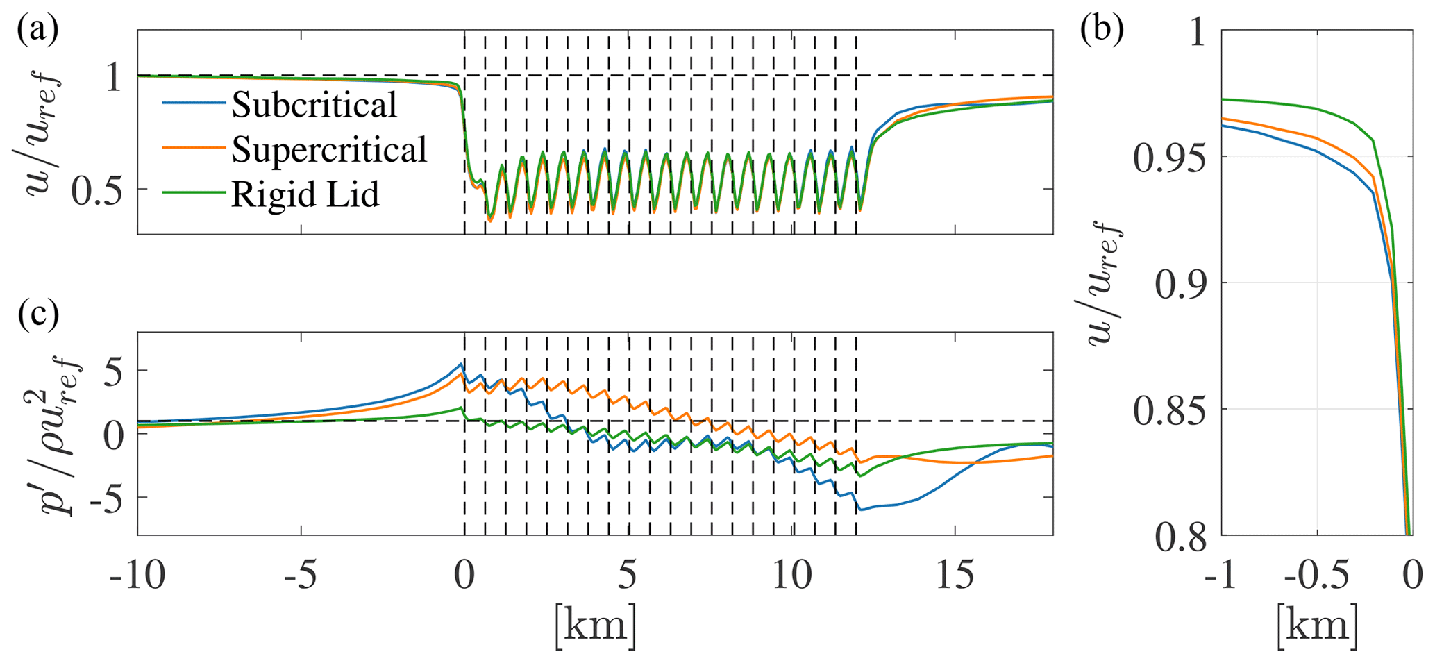
Figure 7 Comparison of velocity magnitude (a) and pressure (c) between subcritical, supercritical, and rigid-lid cases. In (b), a magnification of the differences in velocity magnitude in the wind farm induction region is reported. Data correspond to the AGW-modeled simulations and are averaged both across time (from 105 000 to 140 000 s) and along the wind farm width (from y=0 m to y=3000 m). Pressure data are further averaged vertically between H₁ and H.

Regarding the mean row-averaged power distributions depicted in Fig. 8, it can be stated that, for the simulated conditions, results obtained using the rigid-lid approximation are not far from the subcritical and supercritical figures. In fact, referring to the quantitative data reported in Table 5, the overall wind farm power from the rigid-lid case seems to be in agreement with the simulations featuring AGW effects. The rigid-lid case underestimates the power by 1.5 % compared to the subcritical case and overestimates the power by 3 % with respect to the supercritical case. This trend agrees with the underlying hypotheses of the approximation, where the stronger the potential-temperature jump across the inversion layer, the more it behaves as a rigid lid.

Table 5 Overall wind farm power obtained from LES simulations utilizing subcritical or supercritical conditions or the rigid-lid approximation. The relative differences between the latter and the first two cases are also reported. Time averaging has been performed from 105 000 to 140 000 s in all cases.

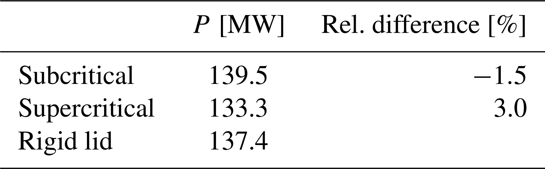
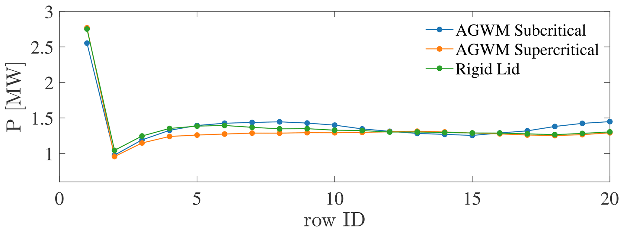
Figure 8 Row-averaged power from the subcritical, supercritical, and rigid-lid cases. Data obtained under subcritical and supercritical conditions are from the AGW-modeled simulations. Time averaging has been performed from 105 000 to 140 000 s in all cases.

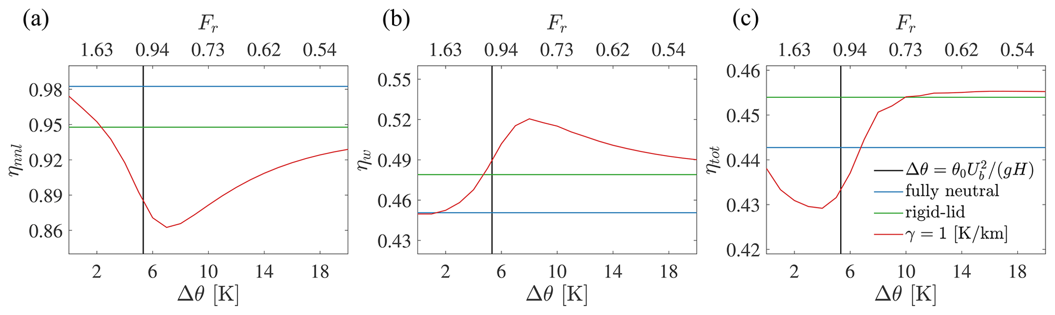
Figure 9 Non-local (a), wake (b), and total (c) wind farm efficiency as a function of Δθ when γ=1 K km⁻¹ (red line). Blue and green lines refer to the fully neutral and rigid-lid cases, respectively. The continuous vertical black line refers to Fr=1. The value of Fr as defined by Eq. (12) is reported on the top axis.

However, the LES results do not provide a clear picture of the relation between the full AGW solution and the rigid-lid approximation, where the effect of Δθ and γ is removed. Notably, removing the effect of H as well leads to the consideration of a fully neutral boundary layer, where vertical streamline displacement is not constrained in any way. To further investigate the relation between these three conditions, the MSC model was used to run a parametric analysis where Δθ and γ were individually varied from 1 to 20 K and from 0 to 20 K km⁻¹, respectively. When varying Δθ, γ was set to 1 K km⁻¹ to match the LESs conducted in this paper. Similarly, when varying γ, Δθ was set to 7.312 and 4.895 K, corresponding to the subcritical and supercritical conditions in this paper, respectively. In addition, two simulations corresponding to the fully neutral and rigid-lid cases were conducted. In the first, Δθ and γ were set to zero, while in the latter, they were set to 1000 K and 1000 K km⁻¹, respectively. The rest of the input parameters were identical to those reported in Table 3. Notably, all cases featured the local blockage model described in Stipa et al. (2024b). For each run, the non-local, wake, and total wind farm efficiencies were evaluated. The power of an isolated wind turbine in the same conditions was calculated by running an additional MSC simulation where the local induction model was removed from the fully neutral setup. This neglects any kind of blockage effect and all first-row turbines produce the same power, taken as P_∞.

For this analysis, it is worthwhile to recall the definitions of the interface Froude number Fr and the parameter P_N, previously defined by Smith (2010), which regulate the physics and magnitude of interface and internal waves, respectively. These can be calculated as

$$\begin{array}{}\text{(12)}& {\displaystyle }& {\displaystyle }Fr={\displaystyle \frac{U_{\mathrm{b}}}{\sqrt{g^{\prime }H}}},\text{(13)}& {\displaystyle }& {\displaystyle }{P}_N={\displaystyle \frac{U_{\mathrm{b}}^{\mathrm{2}}}{NHG}},\end{array}$$

where $g^{\prime }=g\mathrm{\Delta }\mathit{\theta }/{\mathit{\theta }}_{\mathrm{0}}$ is the reduced gravity, and U_b is the bulk velocity inside the boundary layer. Subcritical and supercritical conditions correspond to Fr<1 and Fr>1, respectively, while the importance of internal waves reduces as P_N increases.

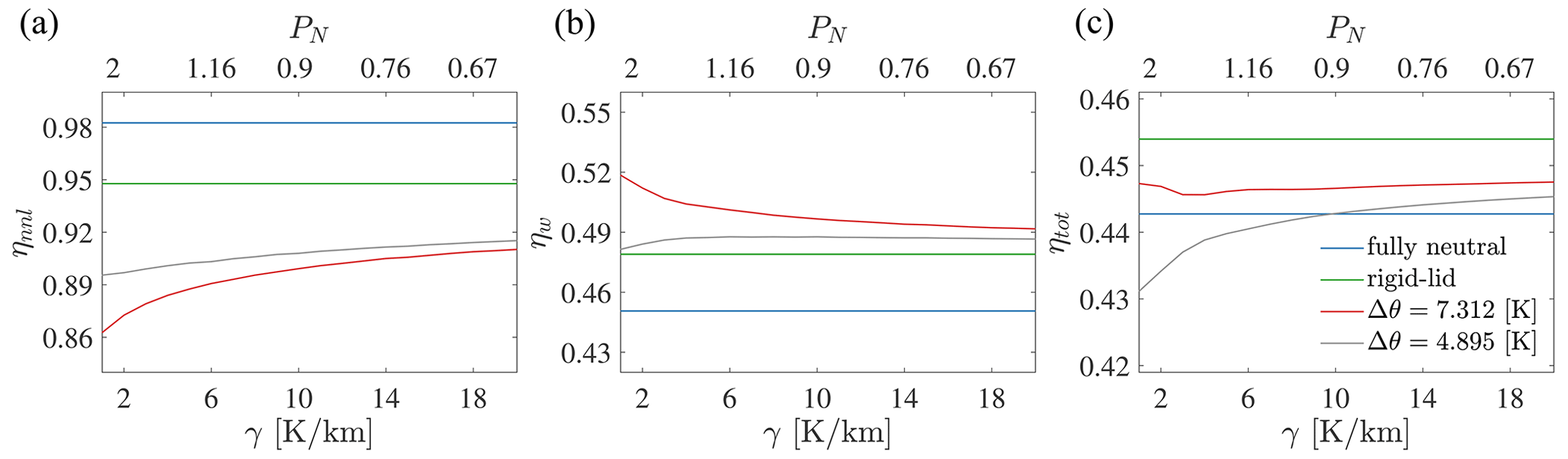
Figure 10 Non-local (a), wake (b), and total (c) wind farm efficiency as a function of γ, with Δθ=7.312 K (red line) and Δθ=4.895 K (gray line). Blue and green lines refer to the fully neutral and rigid-lid cases, respectively. The value of P_N as defined by Eq. (13) is reported on the top axis.

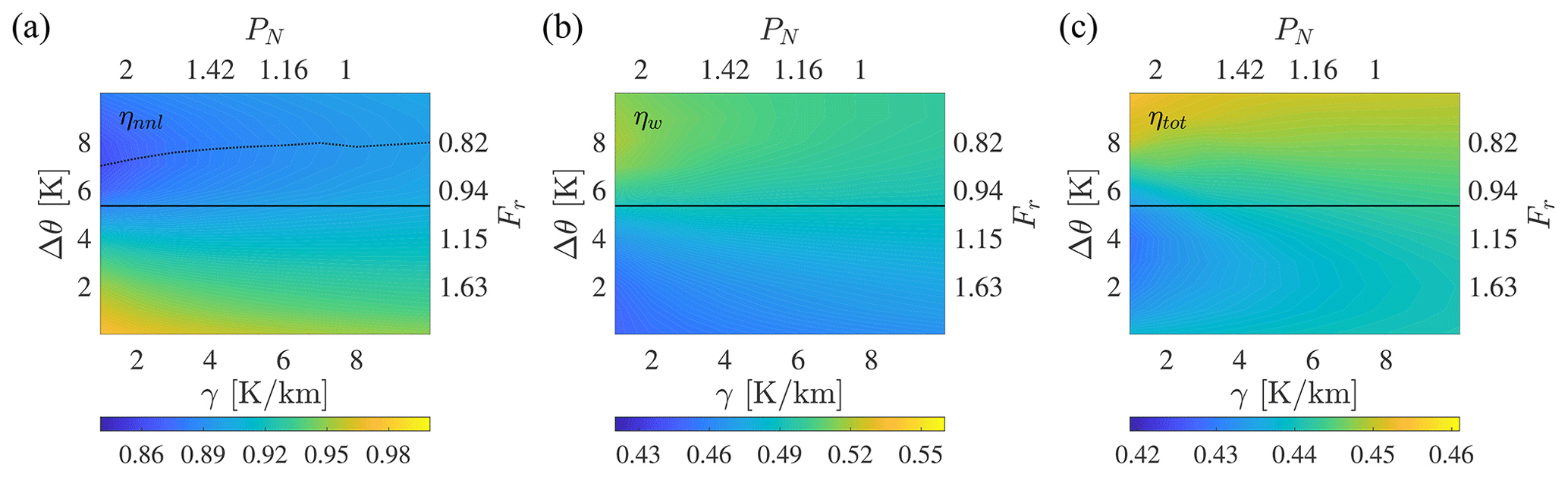
Figure 11 Contours of non-local (a), wake (b), and total (c) wind farm efficiency as a function of Δθ and γ. The continuous horizontal black line refers to Fr=1. The value of Fr as defined by Eq. (12) is reported on the right axis, while the value of P_N as defined by Eq. (13) is reported on the top axis. The dashed line on the plot of η_nnl indicates the locus of minima for the non-local efficiency.

In Fig. 9, the effect of varying Δθ on the wind farm efficiencies is shown. Along the top axis, the inversion strength is converted to Fr using Eq. (12), where U_b is calculated according to Allaerts and Meyers (2019). For low values of Δθ, the non-local efficiency approaches that of a truly neutral case, which is only affected by the combination of individual turbine induction effects. Conversely, when Δθ is large, η_nnl approaches the rigid-lid solution. The transition from these two cases is strongly nonlinear and has a minimum around Fr=1, identified by the continuous vertical line. Interestingly, the minimum of η_nnl occurs for a value of Fr that is slightly lower than unity. For instance, by simplifying the depth-averaged linearized Navier–Stokes equations, Allaerts and Meyers (2019) showed that the second derivative of the total vertical ABL displacement along the streamwise direction, ${\partial }^{\mathrm{2}}\mathit{\eta }/\partial x^{\mathrm{2}}$, is multiplied by a factor $(-\mathrm{1}+F{r}^{-\mathrm{2}}+P_N^{-\mathrm{1}}\mathcal{G})$ (the reader is referred to Allaerts and Meyers, 2019, for the definition of the convolutional operator 𝒢), where Fr is defined by Eq. (12). On the one hand, this provides evidence that the use of the bulk ABL velocity as the characteristic velocity scale for Fr is based on mathematical grounds. On the other hand, as previously noticed by Smith (2010), the term $(-\mathrm{1}+F{r}^{-\mathrm{2}}+P_N^{-\mathrm{1}}\mathcal{G})$ produces a singularity when P_N→∞ (no internal waves). Conversely, when internal waves are present, energy is moved away from the source and the singularity disappears. Hence, referring to a condition where both Δθ and γ are non-zero, our results seem to suggest that the maximum blockage may be observed at $Fr=\mathrm{1}-P_N^{-\mathrm{1}}\mathcal{G}$ (𝒢 is positive upstream of the wind farm) instead of Fr=1, thus indicating a dependence on γ. This behavior can also be noticed in Smith (2010) but has not been mentioned nor discussed further. For our specific case, the minimum of η_nnl corresponds to $\mathrm{\Delta }\mathit{\theta }\approx {\mathit{\theta }}_{\mathrm{0}}{G}^{\mathrm{2}}/\left(gH\right)$, i.e., Fr=1 when this is evaluated with G instead of U_g. Although this may only hold for the conditions adopted in Fig. 9, the drift in the minimum of η_nnl to lower values of Fr as γ increases seems to be a general conclusion, as shown later in Fig. 11. Still referring to Fig. 9, the truly neutral case is characterized by the highest overall non-local efficiency, while the rigid-lid approximation seems to represent a limiting solution for Δθ→∞. In fact, both higher and lower values of η_nnl are obtained for different values of Δθ when considering the full AGW solution. The wake efficiency depicts a reversed behavior, with fully neutral conditions characterized by the lowest overall η_w. Regarding the total wind farm efficiency, this decreases from a value of ≈0.44 in the truly neutral case to ≈0.43 around Fr=1. For increasing values of Δθ, η_tot increases again, overshooting the value corresponding to the rigid-lid case by a small amount (Δη_tot≈0.0013) and slowly approaching it from above when Δθ→∞. However, it is interesting to note that while fully neutral conditions represent the best and worst case scenarios for η_nnl and η_w, respectively, the rigid-lid approximation yields a value of η_tot that is close to the maximum achievable by the wind farm, making it far less conservative. Interestingly, a similar sensitivity analysis performed by Allaerts and Meyers (2019) did not capture such behavior. In fact, while their analysis considered upstream blockage effects, it did not include the beneficial pressure gradient inside the wind farm. As a result, wind farm power is erroneously correlated with the velocity deceleration experienced upstream (i.e., η_tot∝η_nnl).

The behavior of η_nnl, η_w, and η_tot when varying γ with Δθ fixed is somewhat simpler. This is depicted in Fig. 10, where the corresponding value of P_N is also shown on the top axis by converting each γ using Eq. (13). First, it can be noticed that efficiencies are less sensitive to γ than Δθ, and their behavior is simpler than that observed in Fig. 9. Interestingly, the subcritical case shows little dependency of η_tot on γ. In supercritical conditions, the wind farm produces less power than truly neutral conditions for low values of γ (also confirmed by our LESs), while the efficiency is superior when γ≳10 K km⁻¹.

The parametric study was then expanded by systematically computing the wind farm efficiencies for all combinations of Δθ and γ between 0 and 10 K and between 1 and 10 K km⁻¹, respectively, with a unitary step. The results of this analysis, reported in Fig. 11, show that η_tot increases when both Δθ and γ increase, with higher sensitivity to Δθ observed. Notably, conditions where the wind farm extracts more power are also characterized by a large amount of blockage, as testified by the contours of η_nnl. In fact, the decrease in non-local efficiency is compensated for by the effect of the favorable pressure gradient inside the wind farm, which increases η_w. This conclusion also emerges from the analysis presented by Lanzilao and Meyers (2024), where this effect is shown to be more pronounced as the boundary layer height increases. The location, in terms of the values of Δθ and γ, where the minimum η_nnl is experienced is shown in the η_nnl contour. This supports the earlier observation that the minimum of η_nnl corresponds to an Fr value that is slightly lower than 1 and decreases upon increasing the lapse rate. For instance, these results were obtained for an aligned wind farm layout with a fixed number of turbine rows and columns, but they are likely to also depend on the wind farm geometry. However, this is outside of the scope of this paper and represents a subject for future investigation.

To summarize, our results show that the rigid-lid approximation yields a total wind farm efficiency that is close to the maximum achievable by the wind farm, while results obtained under a fully neutral ABL are in the middle of the analyzed conditions. This highlights that AGWs play a crucial role in determining the actual value of η_tot, which is, in general, lower than that observed when only the effect of H is considered. As a consequence, models employing the rigid-lid approximation likely overestimate the wind farm power, while those adopting a fully neutral ABL may over- or underestimate the wind farm power, depending on the structure of the potential-temperature profile.

Finally, the present analysis did not investigate the sensitivity of our results to different values of the inversion height. Nevertheless, based on previous evidence (Lanzilao and Meyers, 2024), AGW effects are expected to fade away with increasing values of H, with both the rigid-lid solution and the full AGW solution likely approaching the fully neutral case.

5 Conclusions

In this study, we introduced an approach that allows the effects of wind-farm-induced atmospheric gravity waves to be modeled without actually resolving these waves in the simulation. The proposed method couples the LES solution below the inversion layer with the MSC model developed by Stipa et al. (2024b). Specifically, the vertical perturbation to the inversion layer produced by the wind turbines, evaluated with the MSC model, is used to vertically deform the top boundary in the LES domain. Since prescribing the inversion displacement automatically establishes the pressure field below, the resulting LES velocity field contains the influence of gravity waves. If CNBLs are simulated, temperature transport becomes irrelevant, as the flow is neutrally stratified inside the domain. AGW feedback with the wind farm is provided by running the MSC model with multiple coupling iterations. The proposed method implies a computational domain that only requires ≈12.7 % of the cells used in the conventional AGW-resolved method. Moreover, referring to finite-volume codes, the simultaneous solution of a concurrent precursor and the use of a fringe region are not required, as there are no gravity waves in the domain. Thus, incoming ABL turbulence can be prescribed using simple inflow–outflow boundary conditions. More generally, tedious and complex measures to avoid spurious gravity wave reflections, such as the Rayleigh damping layer and the advection damping region, are no longer required.

The proposed approach has been verified against the LESs conducted in Stipa et al. (2024b). These are characterized by a setup that allows AGWs to be resolved, and they correspond to subcritical and supercritical regimes of interfacial waves within the inversion layer. The results show that the proposed method is able to capture the impact of gravity waves on pressure and velocity with good accuracy, correctly estimating blockage effects. Moreover, the row-averaged thrust and power distributions are in good agreement with that of the AGW-resolved approach.

Overall, our analysis shows that the proposed AGW-modeled method allows the impact of atmospheric gravity waves on wind farm performance to be modeled at a reduced computational cost and with sufficient accuracy. A drawback of the approach is that its performance depends on how accurately the MSC model captures the displacement of the inversion layer. Moreover, the MSC model is currently limited to stationary and conventionally neutral boundary layers. For this reason, future work will aim at including the internal stability and time dependency in the MSC model, enabling the AGW-modeled method to simulate evolving and arbitrary ABL inflow conditions within the LES at a low computational cost. We also plan on extending the verification of the AGW-modeled approach in different atmospheric conditions using data from Lanzilao and Meyers (2024).

Furthermore, the AGW-modeled method has been used to study the implications of adopting the rigid-lid approximation (Smith, 2024). The latter neglects the inversion layer displacement produced by gravity waves, thus only considering approximated flow confinement effects. While details due to wind farm gravity waves are, as expected, absent, the rigid lid still yields global wind farm blockage and leads to an overestimation (3 % difference) and an underestimation (−1.5 % difference) in overall wind farm power when compared to the supercritical and subcritical cases, respectively, employing the AGW-modeled approach. To further investigate the relation between the full AGW solution, the rigid-lid approximation, and fully neutral conditions (i.e., the absence of stratification), the MSC model has been used to systematically map the error in global wind farm power produced by the rigid-lid approximation under different values of inversion strength and free-atmosphere stratification. The rigid-lid approximation performs worse for supercritical interface-wave regimes (Fr<1) and low values of the lapse rate γ. Conversely, the error reduces with increasing free-atmosphere stability, with greater sensitivity to Δθ than to γ. Truly neutral conditions yield the lowest blockage and the greatest wake effects. The overall wind farm efficiency given by considering the full AGW solution can be lower or greater than the fully neutral case, depending on the vertical potential temperature profile structure, whereas the rigid-lid approximation seems to yield an upper limit for the wind farm efficiency, which increases with increasing free-atmosphere stability. This highlights the importance of considering the potential-temperature profile structure when assessing wind farm performance.

Appendix A: Precursor simulations

This section presents the results of the off-line precursor simulations used to generate the turbulent inflow for the AGW-resolved and AGW-modeled simulations. While they share the same input parameters, reported in Sect. 3, these precursor simulations employ different domain sizes in the spanwise direction. Specifically, a domain of $\mathrm{6}\times \mathrm{3}\times \mathrm{1}$ km was prescribed in the off-line precursors used to initialize the flow in the concurrent-precursor method within the AGW-resolved simulations. Conversely, the off-line precursor conducted to generate the inflow data for the AGW-modeled simulations employed a domain size of $\mathrm{6}\times \mathrm{21}\times \mathrm{1}$ km. Figure A1 reports the horizontally averaged vertical profiles of wind speed magnitude, wind angle, potential temperature, and shear stress for the subcritical and supercritical cases for the two different domain sizes. The inversion jump Δθ, lapse rate γ, reference potential temperature θ₀, inversion width Δh, inversion height H, friction velocity u^*, geostrophic wind G, and geostrophic wind angle ϕ_G are also reported for each case in Table A1. The first five parameters have been obtained by fitting the potential-temperature profile averaged between 100 000 and 120 000 s and between 100 000 and 140 000 s for the AGW-resolved and AGW-modeled cases, respectively, using the Rampanelli and Zardi (2004) model. Since all the simulations employed the potential-temperature controller described in Stipa et al. (2024a), these quantities exactly match across all cases, which is further confirmed by the potential-temperature profiles of Fig. A1. The shear stress profiles also agree almost perfectly, and all cases are characterized by the same final friction velocity u^*. Conversely, the wind speed magnitude and wind angle show some minor differences, which we attribute to the use of the geostrophic damping technique.

Geostrophic damping is used to eliminate inertial oscillations produced by a geostrophic momentum imbalance when initializing the flow without any knowledge about the geostrophic wind. As explained in Stipa et al. (2024a), this situation occurs when one tries to control the horizontally averaged wind velocity somewhere inside the boundary layer. In this case, it is impossible to know what the geostrophic wind will be a priori, and G – which is required in order to apply the geostrophic damping action – has to be retrieved by inverting the equations for the geostrophic balance using the pressure gradient calculated by the velocity controller. In turn, the pressure gradient is calculated by horizontally averaging the wind components at each iteration during the simulation, and thus it is expected that the averaging procedure yields slightly different values when using domains of different sizes. However, the difference between the final values of geostrophic wind for the small and the large domains is only about 0.2 m s⁻¹, which is acceptable in the context of the present study.

Table A1 Inversion jump Δθ, lapse rate γ, reference potential temperature θ₀, inversion width Δh, inversion height H, friction velocity u^*, geostrophic wind G, and geostrophic wind angle ϕ_G evaluated from the off-line precursor simulations used for the AGW-resolved and AGW-modeled cases. The first five parameters have been obtained by fitting the potential-temperature profile with the model of Rampanelli and Zardi (2004) after averaging over time from 100 000 to 120 000 s and from 100 000 to 140 000 s for the AGW-resolved ($\mathrm{6}\times \mathrm{3}\times \mathrm{1}$ km domain) and AGW-modeled ($\mathrm{6}\times \mathrm{21}\times \mathrm{1}$ km domain) cases, respectively.

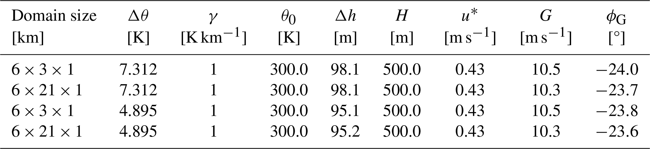
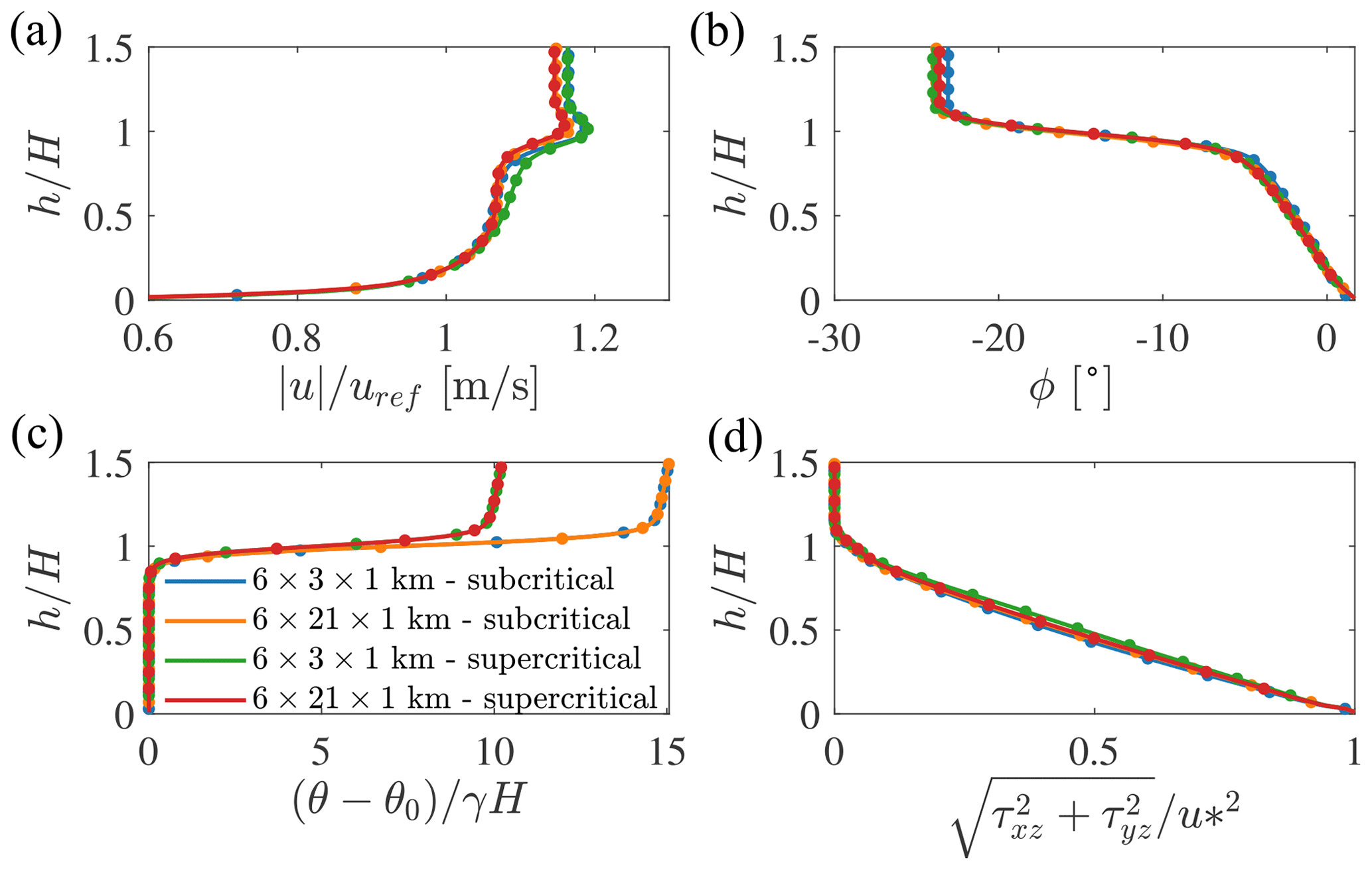
Figure A1 Horizontally averaged and time-averaged wind speed magnitude (a), wind angle (b), potential temperature (c), and shear stress (d) evaluated from the off-line precursor simulations used for the AGW-resolved and AGW-modeled cases. Time averaging has been performed from 100 000 to 120 000 s and from 100 000 to 140 000 s for the AGW-resolved ($\mathrm{6}\times \mathrm{3}\times \mathrm{1}$ km domain) and AGW-modeled ($\mathrm{6}\times \mathrm{21}\times \mathrm{1}$ km domain) cases, respectively.

Appendix B: Effect of atmospheric turbulence on thrust and power averages

As mentioned in Sect. 3, although precursor simulations for the AGW-resolved and AGW-modeled cases shared the same input parameters, they ran in domains of different sizes. As a consequence, while simulations corresponding to the same CNBL conditions produced almost identical horizontally averaged fields (see Appendix A), they featured different realizations of the time-resolved turbulent field. Although this does not represent an issue for the small eddies, large turbulent structures may change the freestream velocity obtained by averaging over a time window when that window is comparable with their size. This is evident from Fig. B1b, which reports the instantaneous wind averaged across the first row of turbines for the AGW-resolved and AGW-modeled approaches corresponding to both subcritical and supercritical conditions. When averaging time histories of, e.g., turbine power or thrust, this effect can introduce a consistent bias, as these quantities depend on the cube and square of the velocity, respectively. Unfortunately, for a time window of the order of the one available in the AGW-resolved simulations (15 000 s), such an effect introduces a variability in wind farm thrust and power that is comparable with the effect of blockage. This is shown in Fig. B1a, where we report the time histories of the velocities sampled at the domain inlet and close to the wind turbine located at the center of the first row for both the subcritical and supercritical AGW-modeled simulations. As can be noticed, the two curves are vertically shifted due to blockage effects. However, even though 15 000 s can be considered a large averaging window, the variations in average velocity obtained by hypothetically shifting this window in time are expected to be comparable with, if not larger than, the vertical shift produced by blockage.

For this reason, when comparing turbine power and thrust between AGW-modeled and AGW-resolved methods under the same CNBL conditions, we choose the averaging window for the former case as follows. First, we ensure that the same window is used for both cases, i.e., 15 000 s, corresponding to the entirety of the data available from the AGW-resolved analyses. Then, we shift the averaging window in the AGW-modeled cases until the freestream velocity averaged among the first-row turbines matches the same quantity obtained from the AGW-resolved simulation. The averaging window resulting from this approach is reported in black in Fig. B1b for both subcritical and supercritical conditions. Finally, the turbine thrust and power from the AGW-modeled cases are averaged over this window, ensuring that the wind farm sees the same inflow velocity in the two cases. We emphasize that this procedure is only applied when looking at turbine data, while the flow variables are always averaged throughout the entire simulation, i.e., from 105 000 to 120 000 s for the AGW-resolved cases and from 105 000 to 140 000 s for the AGW-modeled cases. Although it is true that the approach described above likely forces the average power of the first row to be the same in AGW-resolved and AGW-modeled cases characterized by the same CNBL conditions, it should be recognized that it also allows the thrust and power distributions to vary in the remaining rows. As a consequence, this does not impair our ability to assess the accuracy of the AGW-modeled technique in capturing AGW effects on the row-by-row power production.

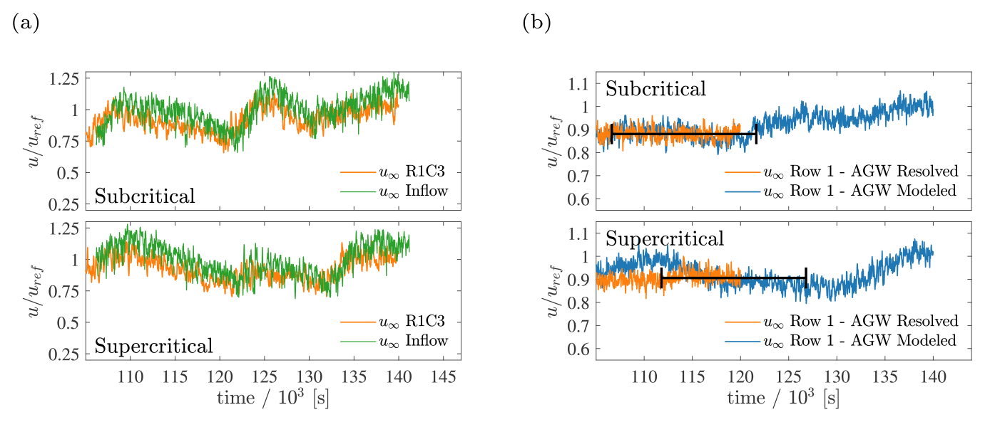
Figure B1 (a) Hub-height wind speed at the domain inlet (green) and as sampled by the wind turbine located in the middle of the first row (orange). Data correspond to the subcritical and supercritical AGW-modeled simulations. (b) Wind speed averaged among the first-row wind turbines for the AGW-resolved (orange) and AGW-modeled (blue) cases. Data corresponding to both subcritical and supercritical conditions are shown. The black bar indicates the time window used to average turbine data in the AGW-modeled simulations when they are compared against the AGW-resolved simulations.