Speeding up large-wind-farm layout optimization using gradients, parallelization, and a heuristic algorithm for the initial layout

As the use of wind energy expands worldwide, the wind energy industry is considering building larger clusters of turbines. Existing computational methods to design and optimize the layout of wind farms are well suited for medium-sized plants; however, these approaches need to be improved to ensure efficient scaling to large wind farms. This work investigates strategies for covering this gap, focusing on gradient-based (GB) approaches. We investigated the main bottlenecks of the problem, including the computational time per iteration, multi-start for GB optimization, and the number of iterations to achieve convergence. The open-source tools PyWake and TOPFARM were used to carry out the numerical experiments. The results show algorithmic differentiation (AD) as an effective strategy for reducing the time per iteration. The speedup reached by AD scales linearly with the number of wind turbines, reaching 75 times for a wind farm with 500 wind turbines. However, memory requirements may make AD unfeasible on personal computers or for larger farms. Moreover, flow case parallelization was found to reduce the time per iteration, but the speedup remains roughly constant with the number of wind turbines. Therefore, top-level parallelization of each multi-start was found to be a more efficient approach for GB optimization. The handling of spacing constraints was found to dominate the iteration time for large wind farms. In this study, we ran the optimizations without spacing constraints and observed that all wind turbines were separated by at least 1.4 D. The number of iterations until convergence was found to scale linearly with the number of wind turbines by a factor of 2.3, but further investigation is necessary for generalizations. Furthermore, we have found that initializing the layouts using a heuristic approach called Smart-Start (SMAST) significantly reduced the number of multi-starts during GB optimization. Running only one optimization for a wind farm with 279 turbines initialized with SMAST resulted in a higher final annual energy production (AEP) than 5000 optimizations initialized with random layouts. Finally, estimates for the total time reduction were made assuming that the trends found in this work for the time per iteration, number of iterations, and number of multi-starts hold for larger wind farms. One optimization of a wind farm with 500 wind turbines combining SMAST, AD, and flow case parallelization and without spacing constraints takes 15.6 h, whereas 5000 optimizations with random initial layouts, finite differences, spacing constraints, and top-level parallelization are expected to take around 300 years.

1 Introduction: wind farm layout optimization

The use of wind energy worldwide increases year by year. The global cumulative wind power capacity reached 837 GW by the end of 2021, with a prediction of around 3200 GW by 2030 (GWEC, 2022). This growth opens the path for the wind energy industry to consider building larger wind farms. The existing literature shows a gap in approaches and strategies to efficiently perform wind farm layout optimization (WFLO) with hundreds of wind turbines. A proper framework to address the problem could enable a faster evaluation of thousands of different configurations, allowing trade-off sensitivity analysis and design insights in a more extensive and faster way.

Since the first work on WFLO by Mosetti et al. (1994) using a gradient-free (GF) approach, the literature on the topic has massively evolved around GF methods. GF-based approaches on the topic include metaheuristic methods such as genetic algorithms (GAs) (González et al., 2018; Wang et al., 2015; Parada et al., 2017), particle swarm optimization (PSO) (Hou et al., 2016; Pillai et al., 2017; Veeramachaneni et al., 2012; Wan et al., 2012; Pookpunt and Ongsakul, 2016), random search (RS) (Feng and Shen, 2017b, a), and many others. GF methods explore the entire design space and may find the global optimum at some point, but processing time explodes with the number of design variables. Therefore, GF methods tend not to scale well for problems with many design variables (Martins and Ning, 2021; Ning et al., 2019) and are more suitable for smaller problems (Wright et al., 1999). Gradient-based wind farm layout optimization (GBWFLO) has been explored more in the last few years. Research in the field has been evolving, including analytical computation of the gradients (Guirguis et al., 2016, 2017; Stanley et al., 2019), a quasi-Newton limited-memory optimizer called limited-memory Broyden–Fletcher–Goldfarb–Shanno (L-BFGS) that estimates the inverse of the Hessian matrix using a generalized secant method (van Dijk et al., 2017; Croonenbroeck and Hennecke, 2021), another limited-memory optimizer called SNOPT (Sparse Nonlinear OPTimizer) that explores the sparsity of the Jacobian matrix (Tingey and Ning, 2017), SNOPT with finite differences (FDs) (Fleming et al., 2016), SNOPT with analytical gradients (Gebraad et al., 2017), and adjoints (King et al., 2017; Allen et al., 2020). Mittal et al. (2016) developed a hybrid GF (GA) and gradient-based (GB) (fmincon) algorithm. A concern regarding GBWFLO is getting stuck in local minima due to the multi-modality of the problem, as visually demonstrated in the literature (Thomas et al., 2022b). One possible strategy to overcome local minima is to perform multi-starts by running multiple optimizations with different initial solutions. Multi-start GBWFLO can explore the design space in a more extensive way, avoiding potential non-optimal final solutions. However, the extra costs to run multi-starts can become another concern for larger problems. In this context, efficient multi-starting is potentially a way of speeding up GBWFLO.

The literature has few articles comparing GF and GB methods in a systematic and standardized way (e.g., with the same configurations). Brogna et al. (2020) performed WFLO in complex terrain with 25 wind turbines, comparing six GF methods with two GB methods that use GlobalSearch and MultiStart from MATLAB optimization toolboxes. They reported GF methods (RS, pattern search, and local search) outperforming the two GB approaches analyzed in terms of both computational costs and optimization results. Croonenbroeck and Hennecke (2021) performed layout optimization to maximize profit and efficiency, which is the ratio between the annual energy production (AEP) and the theoretical maximum AEP. They compared a GB method (L-BFGS-B) against GF algorithms, including modified versions of GA, PSO, simulated annealing (SA), and RS methods. They found L-BFGS-B to perform the fastest among all the options but not with the best results in term of the AEP on a spectrum of six runs. Guirguis et al. (2016) compared GB methods with analytical derivatives and GAs. Additionally, the study compared two GB interior point method (IPM) approaches where one used the FD method to compute the gradients and the other used exact analytical gradients. They found the computational costs of the GB FD approach to be around 20 times higher than the GB approach with analytical gradients. Additionally, the GB approach with analytical gradients resulted in 0.36 % higher wind farm efficiency. Even though the literature is not in total agreement on which approach is the best, GB methods are worthy of further development, especially for large WFLO with many design variables. In order to make GBWFLO more efficient and applicable for large wind farms, the associated computational cost and time need to be properly addressed. The next section will break down the computational cost into different components. In the following sections, approaches to reduce the computational cost are proposed.

2 Total computational time for gradient-based (GB) optimization

Equation (1) shows the total computational time to perform GB optimization. To accomplish faster large GBWFLO, one needs to tackle the bottlenecks of the problem, which are the variables in Eq. (1).

$$\begin{array}{}\text{(1)}& t_{\mathrm{total}}=(t_{\mathrm{iter}}\cdot n_{\mathrm{iter}}+t_{\mathrm{init}})\cdot {\displaystyle \frac{n_{\mathrm{multistarts}}}{n_{\mathrm{cpu}}}},\end{array}$$

where t_total is the total computational time for the GBWFLO; t_iter is the time per iteration; n_iter is the number of iterations until convergence; t_init is the time to initialize the problem, including the time to generate the initial layout, e.g., via Smart-Start (SMAST) from Sect. 3.4.1; n_multistarts is the number of initial starts to avoid getting stuck in local minima, as visually demonstrated in Thomas et al. (2022); and finally, n_cpu is the number of CPU cores available for parallelization of the n_multistarts independent optimizations with different initial layouts.

2.1 Time per iteration

In GB optimization, each iteration typically consists of computing the gradients of the objective function and constraints with respect to all design variables, followed by a line search that comprises one or more function evaluations of the objective and constraints. In this section, we analyze different approaches to reducing the iteration time of GBWFLO.

2.1.1 Gradient computations: analytical vs. finite differences

Computing gradients can be done with different methods. In algorithmic differentiation (AD), all the lines of code are differentiated. These lines are usually composed of simple mathematical operations. AD performs differentiation with respect to each relevant variable at each line of code by applying the chain rule and then sums up all the contributions. The FD method computes the derivatives using a Taylor series expansion, as shown in Eq. (C1) (Appendix C). The FD method computes the Jacobian matrix by looping through all the dimensions to compute the function values, perturbing with a determined step size, and computing the differences in the function. The value of the step size dictates the truncation error. Smaller step sizes reduce the error but increase the amount of numerical noise. The complex-step (CS) method also relies on a Taylor expansion to compute the derivatives. However, the step is represented by an imaginary term in the complex plane (Eq. C3, Appendix C). The CS method typically doubles computational time, as there are 2 times more bits in each value. As shown in Eq. (C4), we need to add a complex step to an input and run $f(x+ih{\widehat{\mathit{e}}}_j)$ to find the gradient with respect to that input. This means that all operations in f, which depends on x, need to be executed on both the real and the imaginary part. The advantage of the CS method is that the only source of error is the truncation error, since there is no associated subtraction cancellation error. Adopting smaller step sizes can reduce truncation errors.

2.1.2 Parallelization

One of the most common objective functions in WFLO is the AEP, which is computed by summing up the contributions of the various combinations of wind direction sectors and wind speeds (referred to as flow cases). The number of flow cases during each iteration is a function of the discretization of the wind resource. To avoid numerical discrepancies, it is necessary to finely discretize the bins of wind directions and wind speeds. The number of flow cases can sum up to 8280 if wind directions and wind speed bins of 1^∘ (0 to 360^∘) and 1 m s⁻¹ (3 to 25 m s⁻¹) are considered, for instance. The contribution of each flow case to the AEP is multiplied by the frequency of occurrence of that combination, and all of them are summed up sequentially in one CPU to calculate the total AEP. As the flow cases are independent, parallelization could speed up iterations because the calculation of AEP contributions of each flow case can be performed simultaneously on several CPUs rather than sequentially on one CPU. Throughout the text, this is referred to as flow case parallelization.

2.1.3 Constraints

Handling constraints in GBWFLO can be done with penalty functions, sequential quadratic optimization (SQP), and IPM (Martins and Ning, 2021). Constraints in GBWFLO usually include physical boundaries and minimal spacing between turbines. Looking at the literature on WFLO, the spacing constraint between turbines varies. Many studies consider 5 wind turbine rotor diameters (D) (Gao et al., 2015; Wang et al., 2015; Parada et al., 2017), but others consider 4 D (Hou et al., 2016; Rodrigues et al., 2015), 3 D (Mittal et al., 2017; Abdulrahman and Wood, 2017), and 2 D (Stanley and Ning, 2019; Padrón et al., 2019; Kirchner-Bossi and Porté-Agel, 2018; Gebraad et al., 2017; Fleming et al., 2016), and a few works consider values beyond 5 D (Rodrigues et al., 2016). When there are too many constraints in optimization, for instance, large WFLO with wind turbine pair-spacing constraints, combining all the constraints into a single constraint, is also possible (Martins and Ning, 2021).

2.2 Number of initial starts

Better initial guesses for the layout can potentially avoid the worst local optima. In the previous literature, the GF approach has been found in some studies to provide better results than multi-start GB approach. However, just a few starts were applied for the GB approach, and the layouts were randomly initialized. It is unclear, for instance, if the work done by Croonenbroeck and Hennecke (2021) to optimize a wind farm with 20 wind turbines could have found L-BFGS outperforming (in terms of the AEP) the GF methods if more multi-start runs had been applied (six runs in this study). Examples of previous studies on multi-starts for GBWFLO considered random multi-starts (Brogna et al., 2020; Yang and Deng, 2023; Thomas et al., 2023; Baker et al., 2019) and Latin hypercube sampling (Guirguis et al., 2016), while an example of a multi-start GF method (RS) also using randomly produced initial guesses is given in Feng and Shen (2017a). A heuristic approach developed by Pérez et al. (2013) assumed turbines were widely spread throughout the wind farm area as a strategy to avoid the wake effects and produce better initial guesses. They generated random regular rectangles, applied a rectangular transformation to extend the points to the wind farm boundaries, and used triangulations to maximize the sum of the areas of the triangles. Still, they had to generate a set of random candidate solutions to initiate the approach. One could enhance heuristic approaches for the initial layout with physics information (e.g., wake effects), avoiding random guesses for the layout. These examples show that there is room for improving multi-start GB methods, for instance, if layouts were initialized using some threshold or method based on physics, rather than being purely random. The Smart-Start (SMAST) algorithm is a heuristic approach based on physics, where wind turbine wake effects guide the decisions to place wind turbines for the initial layout sequentially. SMAST is now available in PyWake (Pedersen et al., 2022), and here we show to what extent the method can improve multi-starting for large GBWFLO. This, in turn, is potentially a way of improving multi-starts for the GB optimization of wind farms, one of the objectives of this present study.

2.3 Objective and scope of the work

This work aims to speed up layout optimization for large wind farms. The strategy is to tackle the bottlenecks in terms of computational expenses. Specifically, on optimization iteration time, the objective is to show how different GB approaches and parallelization of the flow cases scale with the number of wind turbines (n_wt). Moreover, we explore a heuristic approach to produce better initial layout guesses and improve multi-starting, which is necessary for GB methods.

2.4 Contributions to the existing literature

This work intends to complement and add new insights to the existing literature by doing the following:

• Evaluate how parallelization scales with n_wt during large GBWFLO.

• Evaluate how different techniques to compute gradients scale with n_wt when performing GBWFLO.

• Evaluate how n_iter scales with n_wt when performing GBWFLO.

• Demonstrate how n_multistarts scales with n_wt and how to reduce this number using a heuristic approach.

3 Methods

The AEP computations and the optimizations were performed in PyWake (Pedersen et al., 2023) and TOPFARM (Réthoré et al., 2014), which are open-source tools developed by the Technical University of Denmark (DTU). Examples of previous works using PyWake and TOPFARM can be found in the literature (Rodrigues et al., 2022; Ciavarra et al., 2022; Criado Risco et al., 2023; Quick et al., 2023; Pedersen and Larsen, 2020; Nyborg et al., 2023; Fischereit et al., 2021; Pérez-Rúa and Cutululis, 2022). Section 3.1 provides all the relevant details about the optimization formulation. Section 3.2 shows the case studies considered in this work. Section 3.3 describes the methods and assumptions to evaluate iteration time, whereas Sect. 3.4 provides an overview of the heuristic method to produce efficient initial layouts and improve multi-start GBWFLO.

3.1 Optimization: problem formulation

For the AEP computations, an implementation of a Gaussian wake model (Bastankhah and Porté-Agel, 2014) referred to as Bastankhah Gaussian (BG) in Table 1 was considered. The optimization algorithm used in this work is sequential least-squares quadratic programming (SLSQP), which relies on quasi-Newton methods (Powell, 1964; Liu and Nocedal, 1989) and is suitable for constrained GB optimization problems (Wu et al., 2020; Perez et al., 2012; Virtanen et al., 2020). The optimization in this work follows the formulation in Eq. (2), where the objective function is the AEP, and the design variables are the layout coordinates x and y of the turbines. Moreover, farm boundary constraints are applied to restrict the area upon which the turbines can move. TOPFARM handles the design variables and constraints corresponding to the problem formulation in Eq. (2).

$$\begin{array}{}\text{(2)}& \begin{array}{rl}\underset{x,y}{max}\mathrm{AEP}(x,y)& \approx \mathrm{8760}\sum _{d=\mathrm{1}}^{N_{\mathit{\theta }}}\sum _{u=\mathrm{1}}^{N_u}{P}_{d,u}\left(\mathit{x},\mathit{y}\right)\cdot {\mathit{\rho }}_{d,u}\\ & \mathrm{s}.\mathrm{t}.{\mathbf{C}}_{kj}\ge \mathrm{0}\forall k,j,\end{array}\end{array}$$

where C is a matrix of wind farm boundary constraints; d denotes wind directions and u refers to wind speeds, with N_θ and N_u standing for the number of wind directions and wind speeds; P_d,u represents the power output of the wind farm given by the wind turbine coordinate vectors x and y, for wind direction d and inflow wind speed u; and lastly, ρ_d,u is the frequency of wind direction d and inflow wind speed u.

When the wind farm is circular, the boundary constraint, C, is a 1×n_wt matrix, defined in Eq. (3):

$$\begin{array}{}\text{(3)}& {\mathbf{C}}_{k,\mathrm{1}}=R_{\mathrm{wf}}-\sqrt{x_k^{\mathrm{2}}+y_k^{\mathrm{2}}},\end{array}$$

where k is an integer denoting the turbine number, R_wf is the wind farm radius, and the coordinates x and y have the origin at the wind farm center.

When the wind farm span is a parallelogram, the boundary constraints, C, are defined as a 4×n_wt matrix,

$$\begin{array}{}\text{(4)}& {\displaystyle }& {\displaystyle }{\mathbf{C}}_{k,\mathrm{1}}=\left[\left({\displaystyle \frac{x^{\mathrm{UR}}-x^{\mathrm{LR}}}{y_{\max }-y_{\min }}}\right)(y_k-y_{\min })+x^{\mathrm{LR}}\right]-x_k,\text{(5)}& {\displaystyle }& {\displaystyle }{\mathbf{C}}_{k,\mathrm{2}}=x_k-\left[\left({\displaystyle \frac{x^{\mathrm{UL}}-x^{\mathrm{LL}}}{y_{\max }-y_{\min }}}\right)(y_k-y_{\min })+x^{\mathrm{LL}}\right],\text{(6)}& {\displaystyle }& {\displaystyle }{\mathbf{C}}_{k,\mathrm{3}}=y_{\max }-y_k,\text{(7)}& {\displaystyle }& {\displaystyle }{\mathbf{C}}_{k,\mathrm{4}}=y_k-y_{\min },\end{array}$$

where x^UL, x^UR, x^LL, and x^LR are the upper-left, upper-right, lower-left, and lower-right coordinates, respectively, that define the parallelogram boundaries. The upper axis of the parallelogram is assumed to be parallel to the x axis.

As pointed out in Sect. 2.1.3, adopted values of the spacing constraint between wind turbines in a wind farm vary in the literature. A spacing constraint value of 2 D (Eq. 8) was adopted for the layout initialization provided by the heuristic algorithm (described in Sect. 3.4.1) and in the discussion of spacing constraint costs in Sect. 4.1.3. For the remaining optimizations, spacing constraints were disregarded and the formulation of Eq. (2) was adopted. This setup for the spacing constraint is adopted because the cost of handling spacing constraints for each turbine pair does not scale well with n_wt. Additional discussion around the spacing constraint consideration in this work is provided in Sect. 4.1.3, where we provide a plot showing the influence of spacing constraints on speeding up GBWFLO across scales. Moreover, we show in the Discussion section that the minimum spacing in our final results is at least 1.4 D.

$$\begin{array}{}\text{(8)}& \begin{array}{rl}\underset{x,y}{max}& \mathrm{AEP}(x,y)\approx \mathrm{8760}\sum _{d=\mathrm{1}}^{N_{\mathit{\theta }}}\sum _{u=\mathrm{1}}^{N_u}{P}_{d,u}\left(x,y\right)\cdot {\mathit{\rho }}_{d,u}\\ \mathrm{s}.\mathrm{t}.& {\mathbf{C}}_{kj}\forall k,j\ge \mathrm{0}\\ & \sqrt{{\left(x_i-x_j\right)}^{\mathrm{2}}+{\left(y_i-y_j\right)}^{\mathrm{2}}}\ge \mathrm{2}\mathrm{D},\end{array}\end{array}$$

where the sub-indices i and j denote spatial locations.

3.2 Case studies

Two case studies have been considered in this work, which are summarized in Table 1. The power and C_T curves are provided in Fig. 1a and b, respectively. The simulations to investigate the time per iteration were performed with a realistic setup, the Horns Rev 1 wind farm. A Weibull distribution was fitted to the local wind resource (Fig. 1c). We further extended the analysis of Horns Rev 1 to assess how the approaches tested in this work scale with the number of wind turbines n_wt (Fig. 2).

The results for the number of iterations and number of multi-starts are based on more than 55 000 GBWFLOs performed with a faster setup, which uses idealized 3.35 MW wind turbines with constant C_T, site, and wake model definitions from IEA Wind Task 37 case study 1 (IEA Wind Task 37, 2018; Baker et al., 2019). These wind turbines are slightly different than the reference IEA 3.4 MW wind turbines defined by Bortolotti et al. (2019). Extra cases were designed to scale the analysis (Fig. 3). In this simplified setup, only the rated wind speed (9.8 m s⁻¹) is simulated, and all wind turbines operate with constant ${\mathbf{C}}_{\mathrm{T}}\approx \mathrm{8}/\mathrm{9}$. The wake model for these simulations is the Bastankhah Gaussian (BG) with a constant C_T≈0.964 (called simple Bastankhah Gaussian – SBG in Table 1). Another reason for choosing the IEA 37 site is related to the circular boundaries, as rectangular boundaries use 4 times more boundary constraints. Furthermore, Fig. 1d shows the frequency of occurrence of wind directions for the IEA 37 site. Note that, in the current study, we simulate 360 wind directions (as shown in Table 1) while only 16 wind directions were considered in the original IEA Wind Task 37 case study. Our results are, therefore, not directly comparable to the AEP results of the benchmark in Baker's work (Baker et al., 2019). Even though the absolute values (such as the AEP) are not consistent with the original IEA 37, we expect our results on n_iter and multi-starts, as well as the relative comparisons presented in this study, to be valid for more realistic wind farm setups as well.

Table 1 Cases considered for the optimization and the setup and the models used in PyWake/TOPFARM.

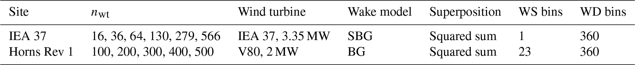
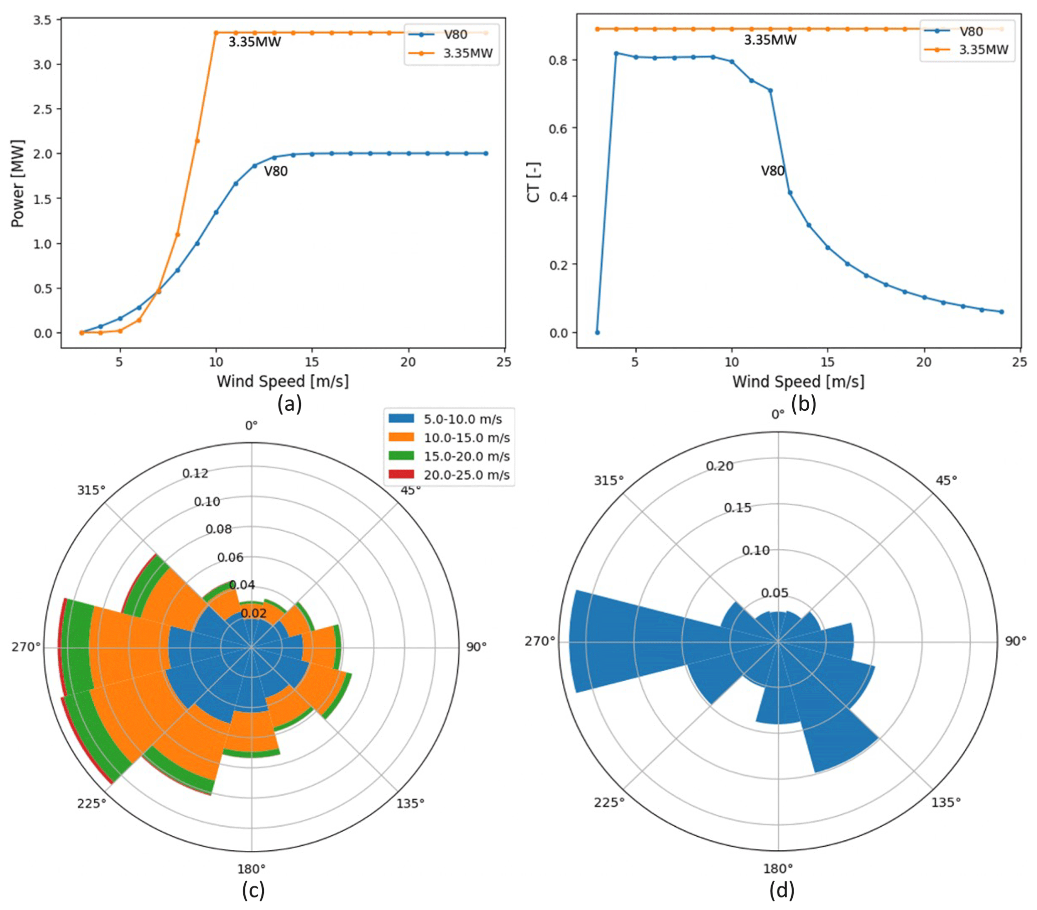
Figure 1 Power curves (a), C_T curves (b), and wind rose distributions for the sites considered in this study: Horns Rev 1(c) and IEA 37 (d).

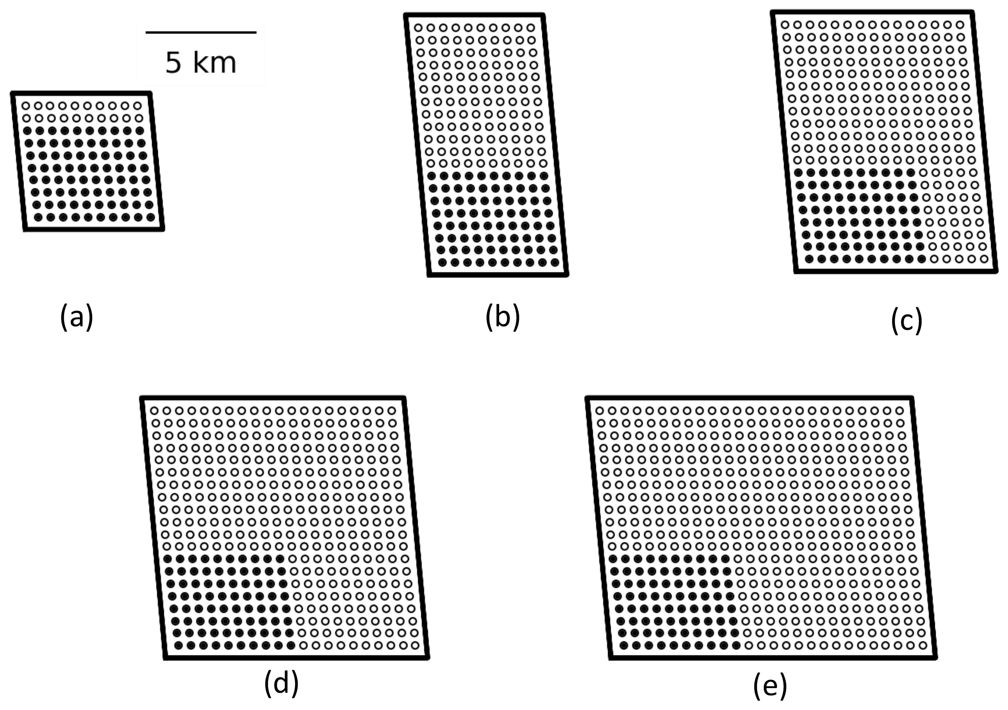
Figure 2 Variations considered in the scaled Horns Rev 1 site with n_wt=100 (a), n_wt=200 (b), n_wt=300 (c), n_wt=400 (d), and n_wt=500 (e). The 80 turbines marked in black are the original turbines from the Horns Rev 1 layout, whereas the turbines marked in white represent the rows and columns added to the original layout.

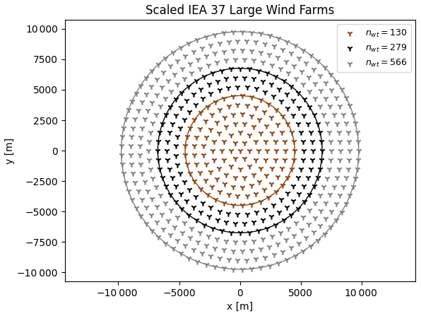
Figure 3 Scaled IEA 37 layouts with R_wf values of 4500, 6750, and 9750 m with n_wt values of 130, 279, and 566, respectively.

3.3 Time per iteration: Horns Rev 1

This section provides the methods implemented to accelerate iteration time during the optimization described in Sect. 3.1. These simulations use a realistic setup (Horns Rev 1), as described in Sect. 3.2 and summarized in Table 1.

3.3.1 Gradient computation

We tested different techniques to compute the gradients and evaluate how they scale with n_wt, including the AD, FD, and CS methods. The theoretical background of these different gradient methods can be found in Sect. 2.1.1, in Appendix C, or in the literature (Martins and Ning, 2021). In this work, we have adapted PyWake to use “Autograd” (Maclaurin et al., 2015) and perform AD to automatically calculate the gradients of the output (AEP) with respect to the inputs (layout coordinates x and y).

3.3.2 Parallelization of the flow cases

This work implemented parallelization in a computational cluster. Single-node operation was utilized with each node being composed of 2× AMD EPYC 7351 CPUs, at 2.9 GHz, with 16 cores and 128 GB of RAM. All the CPUs in each node (32 CPUs per node) are set up to run one simulation. PyWake parallelizes the flow cases, computing chunks of wind directions and wind speeds throughout the several CPUs within a node.

3.4 Number of initial starts: IEA 37

As the total computational time for the GB approach is a function of n_multistarts, this section provides methods for investigating that bottleneck. This work explores a heuristic method (SMAST) to efficiently generate initial layouts for WFLO. The objective of the method is to speed up WFLO by reducing the number of multi-starts necessary to achieve optimized solutions. Section 3.4.1 details SMAST, and Sect. 3.4.2 presents a methodology to improve multi-start GBWFLO based on a comparison between SMAST and a random set of simulations.

3.4.1 The Smart-Start (SMAST) algorithm: a heuristics method

The objective of SMAST is to provide a better initial layout for multi-start GBWFLO. The process is described in Algorithm 1. First, SMAST defines an array ℒ with all the potential positions for wind turbines, in this case a regular grid of points covering the domain. Next, SMAST removes positions from ℒ that do not satisfy constraints, i.e., farm boundary constraints. SMAST then computes the AEP at all the remaining points in ℒ, considering the wakes from the turbines previously added. Next, SMAST randomly selects a point p among the points associated with the highest AEP, ł_best, and places the next turbine at p. Finally, SMAST removes p and all the points that violate the spacing constraint of the newly added wind turbine. This process is repeated until all wind turbines have been placed. As described, SMAST ignores the wake effects of the turbine to be added; i.e., the power reduction in the turbines already added due to wake effects from the new turbine is ignored. This simplification is, however, necessary to make the method feasible. SMAST has a parameter to define the desired degree of randomness (random_pct) when selecting the point p. If SMAST is run without randomness (random_pct=0), the algorithm places the turbine at the point with the highest AEP. In cases where multiple points provide the highest AEP, e.g., in the first iteration assuming a uniform site, the algorithm randomly selects one of these points. This means that even for random_pct=0, the algorithm is able to provide different layouts. SMAST with some randomness (random_pct>0) takes more possibilities for ł_best points and picks one of them randomly. The higher the random_pct is, the more ł_best points are considered. If SMAST is entirely random (random_pct=100), SMAST bypasses the AEP calculation and quickly generates a random layout that satisfies the boundary and spacing constraints. Another parameter that influences the AEP provided by SMAST is the resolution of the grid defined in Algorithm 1. Figures D1 and D2 show examples of SMAST AEP flow maps of the potential positions ℒ with grids with resolutions of 3R and 6R (i.e., the distance between points in ℒ), respectively. Figures D3 and D4 show how the AEP and the computational time vary according to the grid size. The finer the SMAST grid, not only the higher the AEP (except for n_wt=16, where it stabilizes after 4R) but also the higher the computational time of SMAST. The initialization time to generate random layouts (random_pct=100) is nearly negligible compared to, for instance, SMAST with random_pct<100 (Fig. D5), as the expensive loop to compute the AEP and store information about remaining cells in each iteration is bypassed. Memory can also be a problem in running SMAST if the grid is too refined. We do not expect the minimum spacing between turbines in the optimized layout to be sensitive to the grid resolution provided by SMAST, as the optimizer moves the turbines apart to avoid the highest-wake regions.

Algorithm 1 Smart-Start (SMAST) algorithm.

1:

ℒ← {Potential positions for wind turbines}

2:

ℒ←ℒ − OOB_ℒ {OOB: Out of Boundary positions}

3:

P← {initialize empty turbine position vectors}

4:

for i=1 to n_wt do

5:

$Z{}_{\mathcal{L}}\leftarrow \mathtt{AEP}\left(\mathcal{L},P\right)$

6:

min_AEP = random_pctth percentile of Z_ℒ

7:

$l_{\mathrm{best}}=l\in \mathcal{L}$, where Z(l)≥minAEP

8:

p∈_Rl_best, where ∈_R selects a random element

9:

$P=P\cup p$

10:

drop elements of ℒ where $dist(\mathcal{L},p)<\mathrm{2}D$

11:

end for

3.4.2 Random multi-start versus SMAST

Aiming to showcase the capabilities of SMAST to improve multi-starting for GBWFLO, we consider sets of random multi-start simulations with three different IEA 37 case studies: 16, 64, and 279 wind turbines. Those sets are the baseline for the comparisons. The methodology in this work consisted of running 10 000 random simulations (two batches of 5000 simulations) for each case (i.e., randomly generated initial layouts), splitting the results into m chunks and computing the maximum AEP of each chunk. Finally, the mean and confidence intervals of the m maximum values are computed. Figure 4 shows how the normalized optimized AEP varies with the number of random initial starts for the three cases. The AEP is normalized as the average optimal AEP at 5000 initial starts for each batch. As there are two batches with 5000 simulations for each farm size, we take the mean between these two values. The bandwidth in the plots represents the standard deviation within a 99 % confidence interval of the mean. To better clarify the methodology, let us look at the 16-wind-turbine case at 1000 initial starts. The procedure consists in splitting the 10 000 simulations into 10 chunks of 1000 simulations, computing the maximum AEP of each of the 10 chunks, and computing the mean and 99 % confidence interval of these maximum values with Eq. (9). The results from Fig. 4 are used in Sect. 4.3, where we showcase how SMAST improves GBWFLO by achieving the same final optimized results as the random approach (to generate the initial layout) but with a reduced number of multi-starts. Furthermore, what is noticeable in Fig. 4 is that 99.9 % of the maximum AEP is obtained at around 500 starts for n_wt=16, around 2500 starts for n_wt=64, and around 4000 starts for n_wt=279. For small problems, the random approach seems to work as the maximum AEP converges after a relatively low number of starts. Other methods are necessary for larger problems, as the example with n_wt=279 shows, demonstrating that no full convergence is achieved even after 5000 starts. We define convergence when the AEP reaches 99.9 % of the normalized optimized AEP (y axis, Fig. 4). In practice, convergence would mean a flat curve in Fig. 4.

$$\begin{array}{}\text{(9)}& {\mathrm{AEP}}_{\mathrm{ub},\mathrm{lb}}={\mathrm{AEP}}_{\mathrm{mean}}\pm \mathrm{2.576}\cdot {\displaystyle \frac{\mathit{\sigma }}{\sqrt{m}}},\end{array}$$

where AEP_ub and AEP_lb are the upper and lower bounds of the AEP within a 99 % confidence interval, m is the number of chunks, AEP_mean is the mean of the maximum AEP value of each chunk, and σ is the standard deviation of the maximum AEP values.

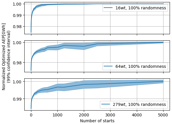
Figure 4 Simulations with initial layout randomly generated for three cases of IEA 37: 16, 64, and 279 wind turbines. These are the baseline cases for comparison with SMAST.

4 Results and discussion

In this section, we present the results of our study on speeding up GBWFLO by exploring each of the variables in Eq. (1). Section 4.1 shows how different gradient computation methods (Sect. 4.1.1) and parallelization (Sect. 4.1.2) impact t_iter. Additionally, the influence of spacing constraints on t_iter is shown in Sect. 4.1.3. Section 4.2 shows how n_iter scales with n_wt. Section 4.3 shows how SMAST can improve n_multistarts for GBWFLO, and finally Sect. 4.4 addresses the impact of these findings on the total optimization time.

4.1 Time per iteration

This section explores t_iter during GBWFLO, as well as strategies to speed up t_iter by different gradient computation methods and parallelization of the flow cases. These results are based on the more realistic Horns Rev 1 setup.

4.1.1 Impact of the gradient computation method

Figure 5a shows the time per iteration for the AD, FD, and CS methods, whereas Fig. 5b shows the speedup when comparing these gradient methods to the FD method. According to Fig. 5a and b, AD computes gradients faster than the FD and CS methods, especially as n_wt increases. AD is around 20 times faster than the FD method for 100 wind turbines, and the speedup increases roughly linearly with n_wt. This is expected and confirms that the FD approach is only feasible for optimizing small wind farms. Figure 5c shows the memory usage for each method, revealing a trade-off between speed and memory. As n_wt increases, AD consumes more memory than the FD and CS methods. AD memory usage is 85 Gb for 500 turbines, which is usually beyond a regular computer's configuration. This value (85 Gb) is more than 4 times higher than for the CS method and around 5 to 6 times higher than for the FD method. The conclusion is that large wind farms (e.g., n_wt=500) can only be optimized with AD, as the FD and CS methods would require CPU usage on the order of years.

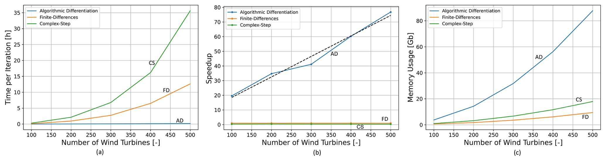
Figure 5 Impact of different gradient computation methods on time per iteration (a), speedup (b), and memory usage (c). The speedup in (b) takes the FD method as the basis for comparisons.

4.1.2 Impact of parallelization

Figure 6a shows the time per iteration for 1, 4, 16, and 32 CPUs, whereas Fig. 6b shows the speedup when comparing these different parallelization schemes. As Fig. 5a and b demonstrated the superiority of AD, the simulations shown in Fig. 6a and b used AD. The speedup computations consider one CPU as the baseline for comparisons. When several multi-starts are needed, our results show top-level parallelization of each optimization to be more efficient than parallelization of flow cases. According to Fig. 6a and b, parallelization makes a positive contribution to reducing t_iter and increasing the speedup. However, the speedup keeps constant with the n_wt. Moreover, the speedup when considering four CPUs against one CPU (Fig. 6b) is 4-fold. The same comparison for 16 CPUs against 1 CPU results in a speedup of around 12-fold, whereas 32 CPUs against 1 CPU have a speedup of around 16-fold. These results indicate that the speedup achieved by parallelizing the flow cases does not linearly increase with the number of CPUs. These results show that parallelization of the multi-start process simulating one seed in one CPU seems more effective than parallelization of the flow cases. This means that if one needs to run hundreds of multi-starts, then better CPU utilization can be achieved by running each multi-start optimization in parallel, i.e., one optimization per CPU. This was confirmed by a small test where 100 multi-starts were optimized. In this test, the flow case parallelization approach was around 2 times slower than the multi-start parallelization approach.

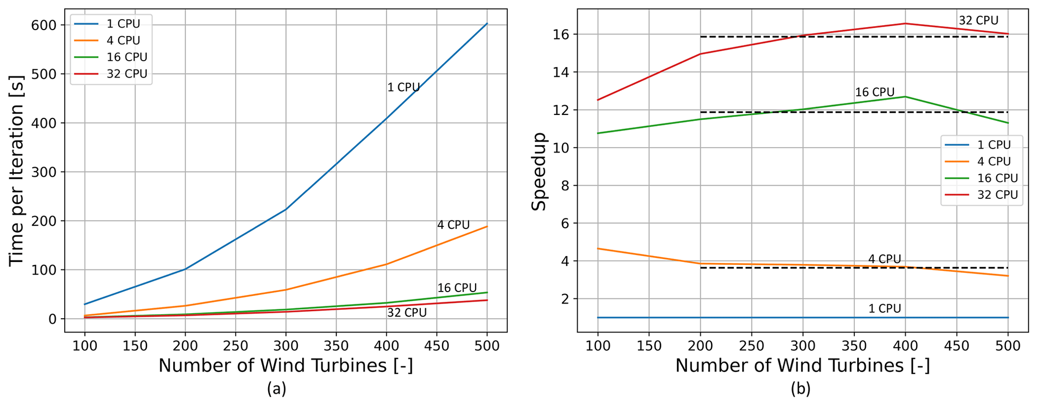
Figure 6 Impact of parallelization of the flow cases on time per iteration (a) and speedup (b) during GBWFLO.

4.1.3 Impact of spacing constraints

Figure 7 shows how the spacing constraint impacts t_iter, indicating that handling spacing constraints does not scale well with n_wt. On the blue curve of Fig. 7, each pair of turbines has an associated minimal spacing that must be satisfied, while the orange line has no pair-spacing constraints. Calculating the spacing between the wind turbines and the associated gradients is relatively fast. The bottleneck is the time spent on handling the constraints inside the optimizer, which is seen to be considerable for large farms. The optimizer used in this work is SLSQP. Calculating the distances between 500 points takes around 0.01 s, and calculating the gradients is similarly fast. SLSQP, however, needs to compute the Lagrangian multiplier for all the constraints, and it is assumed this is what takes most of the almost 2 h increase in the iteration time (Fig. 7) when introducing wind turbine pair-spacing constraints. In this example, handling the spacing constraint of each wind turbine pair in a setup with 500 wind turbines takes roughly 2 h, which slows down the iteration time by a factor of around 10. Obviously, wind turbines must be placed with more than 1 D spacing to avoid a collision, but this minimal distance is implicitly achieved even without spacing constraints in all optimizations performed in this study; see Sect. 4.5, where other issues related to spacing that is too close are also discussed.

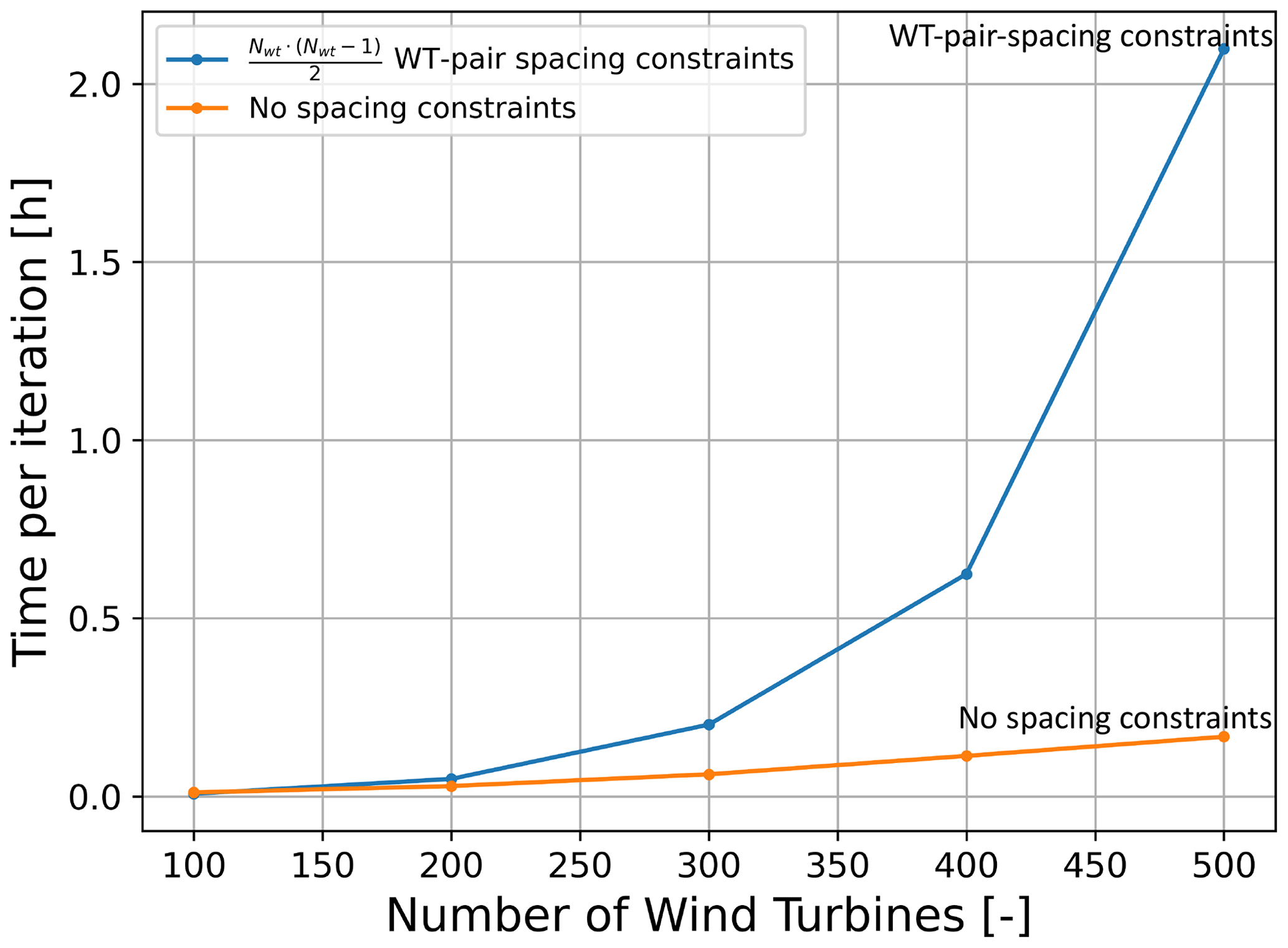
Figure 7 Influence of wind turbine pair-spacing constraints on time per iteration during GBWFLO.

4.2 Number of iterations

The results in this section are based on optimizations of the faster scaled IEA 37 case study, described in Sect. 3.2.

Figure 8 shows the n_iter to achieve convergence as a function of n_wt based on 5000 optimizations of each farm size, $n_{\mathrm{wt}}=\mathit{\{}\mathrm{16},\mathrm{36},\mathrm{64},\mathrm{130},\mathrm{279}\mathit{\}}$. The mean n_iter is seen to scale linearly with n_wt: $n_{\mathrm{iter}}=\mathrm{2.3}{n}_{\mathrm{wt}}+\mathrm{16}$. The linear fit of the median has the same slope as Fig. 8 with just one decimal difference. Additionally, two optimizations were performed with 566 wind turbines to verify the linear extrapolation to larger wind farm sizes.

In some cases n_iter is considerably higher than the mean. We suspect that these outliers represent cases where the optimizer gets stuck in local minima.

In this case, n_iter scales almost perfectly linearly with 2.3 times n_wt, but in general we expect n_iter to be highly dependent on the optimizer; its settings, e.g., tolerance; the nature of the objective function and the constraints, e.g., the shape of the boundary; and the scaling of the input, the objective function, and the constraints. More investigation is needed to make a general conclusion.

The 5000 optimizations of each farm size were performed with different levels of randomness (1000 each), random${}_{\mathrm{pct}}=\mathit{\{}\mathrm{0},\mathrm{1},\mathrm{10},\mathrm{50},\mathrm{100}\mathit{\}}$, but it was found that the amount of randomness only has a minor impact on the number of iterations; see Fig. E2 in Appendix E.

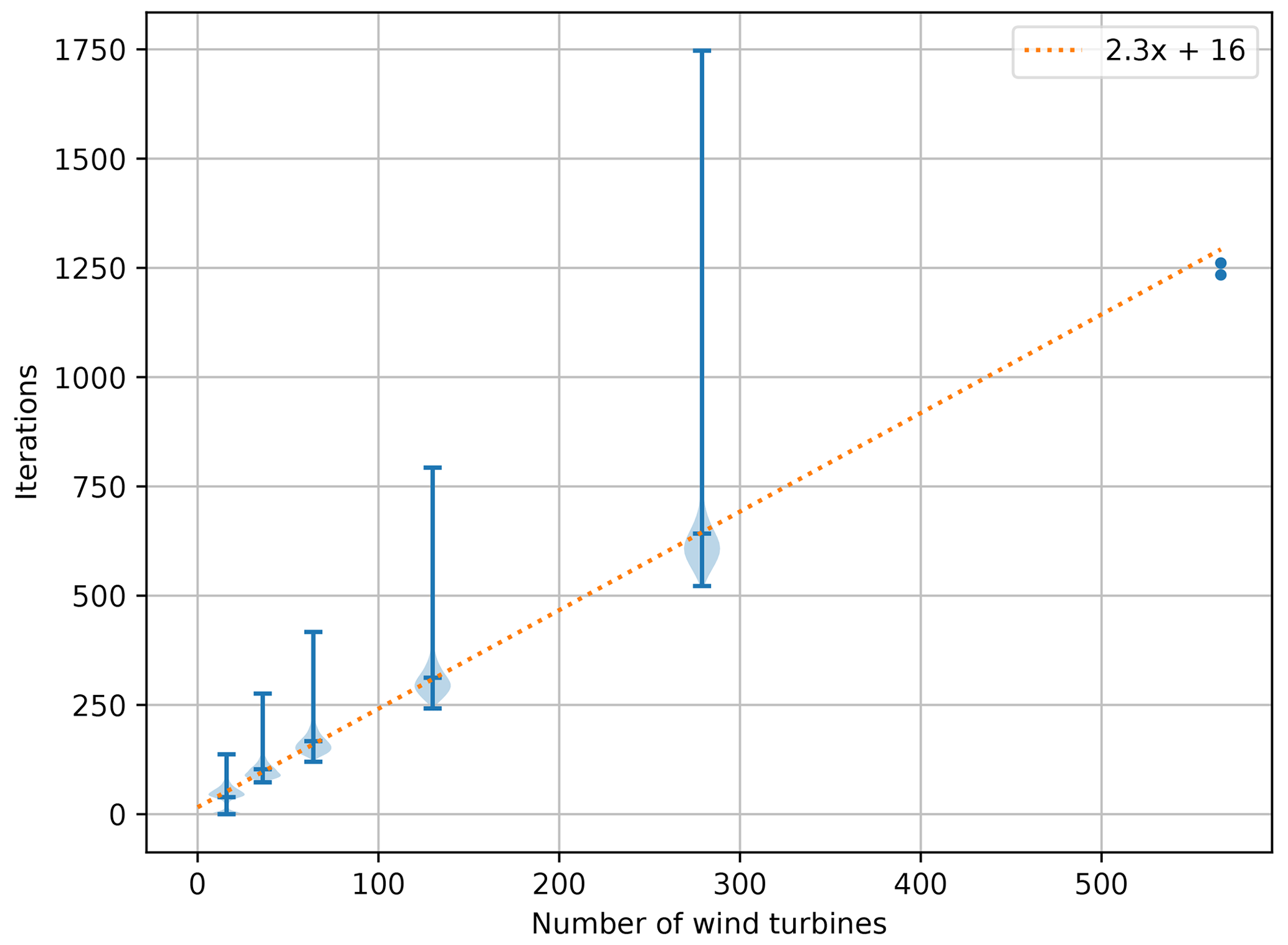
Figure 8 Number of iterations as a function of the number of wind turbines to achieve convergence. The site considered is the scaled IEA 37.

4.3 Number of initial starts

The results on reducing the number of initial starts presented in this section are based on simulations of the scaled IEA 37 study case described in Sect. 3.2. Our approach used a heuristic algorithm to improve the multi-start GBWFLO optimization by providing a better guess for the initial layout. Section 3.4.1 describes how the SMAST algorithm sequentially places turbines in a gridded physical domain to obtain an initial layout. The SMAST algorithm evaluates the wind resource of each grid cell before placing each new turbine. The more refined the grid is, the more expensive it is to run SMAST. Before studying how to improve the multi-start method, we ran a batch of simulations to check the sensitivity of SMAST to several metrics (Appendix D and E, Figs. D3, D4, E1, E2). The initial AEP provided by SMAST increases as the grid resolution becomes finer (as mentioned in Sect. 3.4.1); however, there is a limit at which the AEP no longer increases significantly (Figs. D3 and D4). Based on the results, the SMAST grid resolution adopted in this study is 3R (i.e., 3 times the wind turbine radius) for all the cases, except the 566-wind-turbine case, where 5R was adopted to prevent memory problems. These resolution values provide, at the same time, a suitable initial AEP at reasonable computational expense. To get a sense of SMAST computational time for large wind farms, Table 2 shows a summary of the mean time of SMAST and the AEP gain, which is the percentage of improvement comparing the initial mean AEP provided by SMAST with random_pct=0 and random_pct=100. The computational time for the smallest case n_wt=16 is not high (only 3 s), but it does not scale well and gets up to around 3 h for the largest case in which n_wt=566.

Table 2 SMAST computational time and gain for the IEA 37 cases considered.

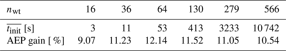
Figure 9 shows how the optimized AEP varies as a function of n_multistarts, considering different levels of randomness (random_pct) for SMAST and different n_wt values. The dashed black lines in each plot show the maximum AEP and the gray bands a 99 % confidence interval of the best result for the optimized AEP among two sets of 5000 simulations with entirely random initial layouts (random_pct=100). In the 16-wind-turbine case, Fig. 9a, the random approach is equal or superior to SMAST for all levels of randomness. In the 64-wind-turbine case, Fig. 9b, SMAST with 0 % randomness needs only one start to obtain an AEP result that is as high as the best of 5000 multi-start optimizations with 100 % randomness. SMAST with 1 % and 10 % requires 2 and 122 initial starts (2–3 and 53–414, respectively, within a 99 % confidence interval), respectively, to surpass the 100 % random case with 5000 starts. It is also seen that for more than 80 starts, 1 % randomness improves the AEP result. The 279-wind-turbine case, Fig. 9c, shows that the 0 % and 1 % SMAST cases need one initial start to surpass the 100 % random case, whereas the SMAST 10 % case requires approximately eight initial starts (4–16 within a 99 % confidence interval). Note, however, that even though one start with 0 % randomness is enough to surpass the random case, it may still be beneficial to run the simulation with multiple starts. In this example, the maximum AEP can be increased by approximately 0.5 % by running 30 starts instead of 1.

These results indicate that more randomness gives a higher AEP for a sufficiently high number of starts – the larger the farms and the greater the randomness, the more starts are needed. For the small n_wt=16 case, “sufficiently high” is fewer than 20 starts. For the medium n_wt=64 case, 80 starts are enough for 1 % randomness, while more than 500 starts are needed when introducing more randomness. For the large 279-wind-turbine farm, sufficiently high is far beyond 500, even for the 1 % randomness case. In summary, SMAST significantly reduces the number of starts required to obtain a high AEP result compared to the random approach when optimizing large-wind-farm layouts. Moreover, a randomness value (random_pct) lower than 100 % means that the initial layout is limited to a subset of the design space. If the optimizer is not able to escape the local minima, this may also limit the solution space. For small wind farms, a higher AEP may be found by a random guess in the solution space that is not accessible when using less randomness in the initial start. For larger wind farms, finding a better solution by randomness is not realistic.

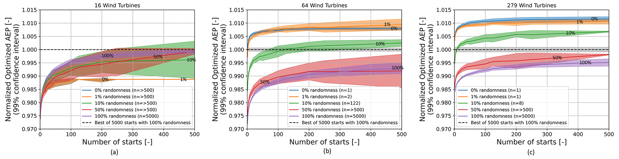
Figure 9 Normalized optimized AEP as a function of the number of initial starts, considering the IEA 37 case study. (a) Normalized optimized AEP, 16 wind turbines; (b) normalized optimized AEP, 64 wind turbines; (c) normalized optimized AEP, 279 wind turbines. The “n” variable refers to the number of initial starts at which the SMAST approach results in higher normalized optimized AEP, as compared to 10 000 simulations, which used an approach with layouts randomly initialized.

4.4 Total computational time

This section summarizes the potential reduction in the total optimization time, t_total, for a wind farm with 500 wind turbines by using all the strategies detailed in this work. The t_total is estimated using Eq. (1) and combines the iteration time found with the more realistic setup (Horns Rev 1) with the number of iterations and multi-starts found with the faster IEA 37 setup. Additionally, we assume that the result regarding the number of multi-starts for 279 wind turbines is similar for a wind farm with 500 wind turbines.

First, the time per iteration for 500 wind turbines using the FD method and one CPU without spacing constraints is 12.6 h (see Fig. 5a). Additionally, the time for computing and handling spacing constraints for 500 wind turbines was found to be 1.9 h (see Figs. 7 and 6a). Therefore, the total iteration time without the methods proposed in this work is 14.5 h. The number of iterations for a 500-wind-turbine case is estimated to be 1166 using the linear equation found in Sect. 4.2. In this case, we set the number of random multi-starts to 5000, which is not even enough to get a result as good as one optimization with SMAST if the trend from Fig. 9 continues up to 500 wind turbines. Hence, the total optimization time on one node with 32 CPUs is estimated to be $\mathrm{14.5}\mathrm{h}/\mathrm{iter}\cdot \mathrm{1166}\mathrm{iter}\cdot \mathrm{5000}\mathrm{starts}/\mathrm{32}\mathrm{CPUs}\approx \mathrm{300}\mathrm{years}$.

Applying the methods presented in this work, i.e., AD, flow case parallelization on 32 CPUs, and no spacing constraints, the time per iteration is reduced to 38 s (see Fig. 6a). Using SMAST, one optimization is expected to give a higher AEP than the approach described above. The time to generate an initial layout by SMAST is ≈3.3 h. Therefore, the total optimization time is 38 s$/$iter ⋅1166 iter+3.3 h ≈ 15.6 h.

A slightly higher AEP can be obtained by running, e.g., 32 optimizations with SMAST. In this case, it is more efficient to parallelize the starts rather than the flow cases. The iteration time is thereby increased to 603 s (see Fig. 6a), and the total optimization time becomes $(\mathrm{603}\mathrm{s}/\mathrm{iter}\cdot \mathrm{1166}\mathrm{iter}+\mathrm{3.3}\mathrm{h})\cdot \mathrm{32}\mathrm{starts}/\mathrm{32}\mathrm{CPUs}\approx \mathrm{199}\mathrm{h}$.

4.5 Discussion

When running GBWFLO for large wind farms, one critical aspect is the spacing constraint. As previous works in WFLO considered small to medium wind farms, this problem was not explicitly apparent. That is why this work applied spacing constraints only to generate the initial layout (by SMAST) and disregarded them for the remaining optimization. That considerably reduced the computational expenses to achieve the objectives of this study. This was only possible because the wind turbines did not end up being too close to each other. The strategy adopted in this work relied on the inherent behavior of wind turbine wake models, which places turbines apart from each other to produce more AEP, guiding the optimizer driver towards separating them. As the objective of the work is to show the impact of different gradient computation methods, parallelization, and the capabilities of SMAST, we do not expect disregarding the constraints to affect the results. For all the optimizations, the turbines were at least 1.4 D separated apart in the final optimized designs, which is lower than typical spacing distances. It is crucial, though, to reinforce that placing turbines too close to each other can cause problems related to mechanical loads on wind turbine components. Additionally, the applied engineering wake models do not include a dedicated near-wake model, and their behavior close to the turbine is therefore missing some physical aspects. Furthermore, the constraint handling problem may be solved by constraint aggregation, but initial investigations showed a negative impact on the optimized AEP. Therefore, we decided to run the optimizations in this study without spacing constraints and leave the in-depth investigation of spacing constraint aggregation for future work.

In this work, the driver used for the optimization is the open-source SLSQP. The choice for this driver has to do with the possibility of a fully open-source simulation tool (even though other tools such as IPOPT could have been used). PyWake and TOPFARM, as mentioned in Sect. 3, are open-source packages developed by DTU and well coupled with SLSQP. Additionally, SLSQP is currently commercially used by the wind energy industry to perform GBWFLO. The literature shows, though, some studies pointing towards the superiority of SNOPT for optimal AEP (Baker et al., 2019; Thomas et al., 2022). Therefore, future work could use SNOPT or another driver to confirm the trends found in this work.

Another possibility of speeding up wind farm optimization is to consider a subset of the flow cases. For wind farm AEP computations, Thomas et al. (2022) demonstrated that at least 40 or 50 wind sectors are necessary to run WFLO. However, wriggles can occur when simulating too few wind directions. We define wriggles as direction-dependent variations in wind turbine wakes when averaging all the wind directions with their sector frequency weight. In simple cases, the occurrence of such wriggles has been found to drastically increase the number of local minima. Taking this into consideration, in this work, we took the conservative approach of considering wind direction bins of 1^∘. However, we acknowledge other possibilities and intend to explore them in future work.

5 Conclusions

In this work, different strategies to accelerate WFLO of large wind farms with hundreds of turbines have been explored. We have focused on GB approaches as GF methods tend to scale poorly for problems with many design variables. We have separated the problem into reducing the iteration time, the number of iterations, and the number of multi-starts (optimization with different initial layouts).

The time per iteration has been investigated using a realistic setup with scaled versions of the Horns Rev 1 wind farm (100–500 wind turbines). It was found that the iteration time can be decreased by computing gradients via AD compared to the FD and CS methods. The speedup scales linearly with the number of wind turbines and was found to be around 75 times for a wind farm with 500 wind turbines. However, on personal computers or for even larger farms, AD may become unfeasible due to its extensive memory requirements.

Simulating the different flow cases in parallel is another approach to reducing the iteration time, but the speedup was found to be roughly constant with the number of wind turbines. Moreover, top-level parallelization was found to be more efficient. In general, we therefore recommend using the available CPUs to parallelize multi-starts with different initial layouts instead of flow cases.

Requiring all pairs of wind turbines to be separated by some minimum distance introduces a considerable number of optimization constraints. The time used to handle these constraints by the applied SLSQP optimizer scales very badly with the number of wind turbines, dominating the iteration time of wind farms with 300 wind turbines or more. The problem may be solved by using another optimizer or by constraint aggregation, but in this study, we ran the optimizations without spacing constraints and observed that all pairs of wind turbines were separated by at least 1.4 D in all optimizations.

The number of iterations needed to achieve convergence was investigated using a faster setup (IEA 37 with up to 566 wind turbines). The mean number of iterations was found to scale linearly with the number of wind turbines times 2.3. This result is assumed to be highly dependent on the optimizer; its settings; the boundary shape; and the scaling of the inputs, outputs, and constraints. The heuristic Smart-Start (SMAST) approach, which was used to obtain better initial layouts, did not manage to reduce the number of iterations significantly.

The number of multi-starts, i.e., number of optimizations performed with different initial layouts to obtain a result close to the global maximum, was also investigated using the faster setup (IEA 37 with up to 279 wind turbines). The number of multi-starts needed to reach 99.9 % of the best AEP from 10 000 optimizations was found to depend on the wind farm size: 500 starts for 16 wind turbines, 2500 starts for 64 wind turbines, and 4000 starts for 279 wind turbines. For the biggest wind farm, however, it is suspected that 10 000 optimizations would not be enough to find the global maximum.

Comparing SMAST with different levels of randomness (random_pct=0–100) revealed that more randomness in the initial layouts gives a higher AEP when optimizing small wind farms (16 wind turbines), while less randomness, i.e., better initial layouts, is superior for large farms (64 and 279 wind turbines). It was found that the AEP obtained from one optimization initialized with SMAST (random_pct=0) was higher than the best AEP of 5000 optimizations initialized with random wind turbine positions (random_pct=100). It is expected that the superiority of SMAST will increase even further for larger wind farms.

The reduction in total optimization time is estimated, assuming that the result regarding the number of multi-starts for 279 wind turbines is similar for larger wind farms and that the number of starts and iterations found using the faster IEA 37 setup can be combined with the iteration time from the more realistic Horns Rev 1 setup. It was estimated that running one optimization with SMAST, AD, and flow case parallelization and without spacing constraints instead of 5000 optimizations with random initial layouts, the FD method, spacing constraints, and top-level parallelization reduces the total optimization time from around 300 years to 15.6 h while increasing the AEP.

We suggest future works on large WFLO to explore the effect of constraint aggregation methods on iteration time and the optimized AEP and to test the proposed approaches with other optimizers and wind farm setups to generalize the results of this present work.

Appendix A: Abbreviations and acronyms

AEP	Annual energy production
AD	Algorithmic differentiation
SMAST	Smart-Start
GWEC	Global Wind Energy Council
WFLO	Wind farm layout optimization
GF	Gradient-free
GA	Genetic algorithm
PSO	Particle swarm optimization
RS	Random search
GBWFLO	Gradient-based wind farm layout optimization
L-BFGS	Limited-memory Broyden–Fletcher–Goldfarb–Shanno
SNOPT	Sparse Nonlinear OPTimizer
FDs	Finite differences
CS	Complex step
GB	Gradient-based
SA	Simulated annealing
IPM	Interior point method
SQP	Sequential quadratic optimization
BG	Bastankhah Gaussian
SBG	Simple Bastankhah Gaussian
SLSQP	Sequential least-squares programming
OOB	Out of boundaries

Appendix B: Nomenclature

titer	Time per iteration
nmultistarts	Number of multi-starts
niter	The number of iterations until convergence
ttotal	Total computational time for the GB approach
nwt	The number of wind turbines in a wind farm
x	Layout coordinate of the wind turbine in the x direction
y	Layout coordinate of the wind turbine in the y direction
Ck	Wind farm boundary constraint
k	Integer number to represent the index of C and the turbine number
d	Wind direction
u	Wind speed
Nθ	Number of wind directions
Nu	Number of wind speeds
Pd,u	The power output of the wind farm given by the wind turbine coordinate vectors x and y
ρd,u	The frequency of wind direction d and inflow wind speed u
Rwf	Wind farm radius
xUL	Upper-left coordinate that defines the parallelogram boundaries
xUR	Upper-right coordinate that defines the parallelogram boundaries
xLL	Lower-left coordinate that defines the parallelogram boundaries
xLR	Lower-right coordinate that defines the parallelogram boundaries
CT	Thrust coefficient
WS bins	Bins for the wind speeds
WD bins	Bins for the wind directions
ℒ	Vector of potential positions for wind turbines
łbest	Points in ℒ with the highest AEP
p	Point among łbest
OOB	Points out of the boundaries of the wind farm
P	Wind turbine position vector
randompct	Level of randomness for layouts generated by SMAST
D	Wind turbine diameter
AEPub	The upper bound of the AEP within a 99 % confidence interval
AEPlb	The lower bound of the AEP within a 99 % confidence interval
m	The number of chunks of the 10 000 simulations with initial layouts randomly generated
AEPmean	The mean of all the maximum AEP values of each chunk m
σ	Standard deviation of the maximum AEP values of all chunks of size m

Appendix C: Equations for gradient computations

Equation (C1) shows the FD generalized formula containing all the high-order truncation terms for the forward difference. Equation (C1) reduces to Eq. (C2) when considering only the first-order truncation terms, where O(h) refers to the truncation error.

$$\begin{array}{}\text{(C1)}& f(x+h{\widehat{\mathit{e}}}_j)=f\left(x\right)+h{\displaystyle \frac{\partial f}{\partial x_j}}+{\displaystyle \frac{h^{\mathrm{2}}}{\mathrm{2}\mathrm{!}}}{\displaystyle \frac{{\partial }^{\mathrm{2}}f}{\partial x_j^{\mathrm{2}}}}+{\displaystyle \frac{h^{\mathrm{3}}}{\mathrm{3}\mathrm{!}}}{\displaystyle \frac{{\partial }^{\mathrm{3}}f}{\partial x_j^{\mathrm{3}}}},\mathrm{\dots },\end{array}$$

where h represents the FD step size and ${\widehat{\mathit{e}}}_j$ is the unit vector in the jth direction, as shown by Martins and Ning (2021).

$$\begin{array}{}\text{(C2)}& {\displaystyle \frac{\partial f}{\partial x_j}}={\displaystyle \frac{f(x+h{\widehat{\mathit{e}}}_j)-f\left(x\right)}{h}}+O\left(h\right),\end{array}$$

where O(h) represents the truncation error.

Similarly to the FD method, for the CS method, Eq. (C3) reduces to Eq. (C4) when disregarding higher-order truncation terms.

$$\begin{array}{}\text{(C3)}& {\displaystyle }f(x+ih{\widehat{\mathit{e}}}_j)=f\left(x\right)+ih{\displaystyle \frac{\partial f}{\partial x_j}}+{\displaystyle \frac{h^{\mathrm{2}}}{\mathrm{2}\mathrm{!}}}{\displaystyle \frac{{\partial }^{\mathrm{2}}f}{\partial x_j^{\mathrm{2}}}}+i{\displaystyle \frac{h^{\mathrm{3}}}{\mathrm{3}\mathrm{!}}}{\displaystyle \frac{{\partial }^{\mathrm{3}}f}{\partial x_j^{\mathrm{3}}}},\mathrm{\dots }\text{(C4)}& {\displaystyle \frac{\partial f}{\partial x_j}}={\displaystyle \frac{\mathrm{Im}\left(f\right(x+ih{\widehat{\mathit{e}}}_j\left)\right)}{h}}+O\left(h^{\mathrm{2}}\right)\end{array}$$

Appendix D: Grid resolution

For the charts on the left in Figs. D1 and D2, the AEP is calculated for a wind turbine with all potential positions, taking into account wakes from the wind turbine(s) already added (in black color). A new wind turbine (red) is added at the best position. The chart on the right shows the final layout provided by SMAST, where all 64 wind turbines have been placed.

Figure D1 Example of a SMAST grid with 3R resolution for n_wt=64.

Figure D2 Example of a SMAST grid with 6R resolution for n_wt=64.

Figure D3 SMAST grid resolution for the small and medium wind farms.

Figure D4 SMAST grid resolution for the large wind farms.

Figure D5 Layout initialization time comparison using SMAST.

Appendix E: Random parameter impact

Figure E1 Impact of random_pct on the initial AEP.

Figure E2 Impact of random_pct on the number of iterations.

Appendix F: Final AEP and optimization time

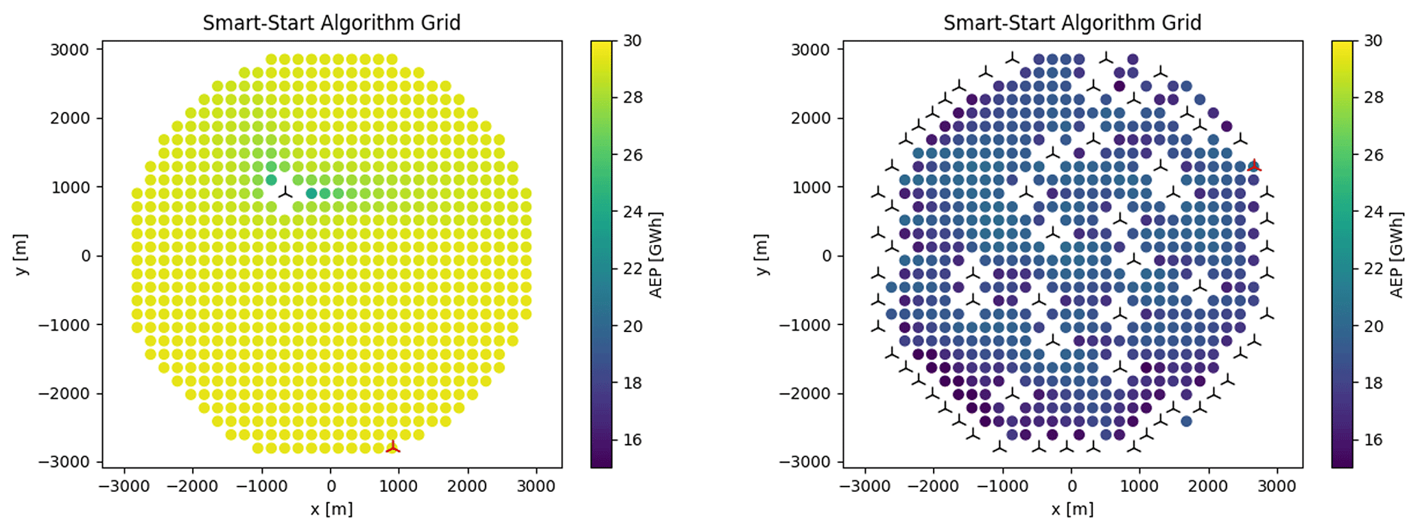
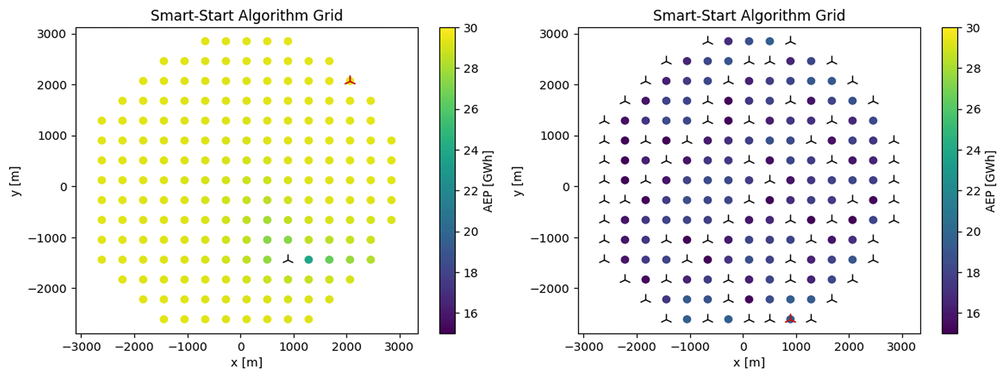
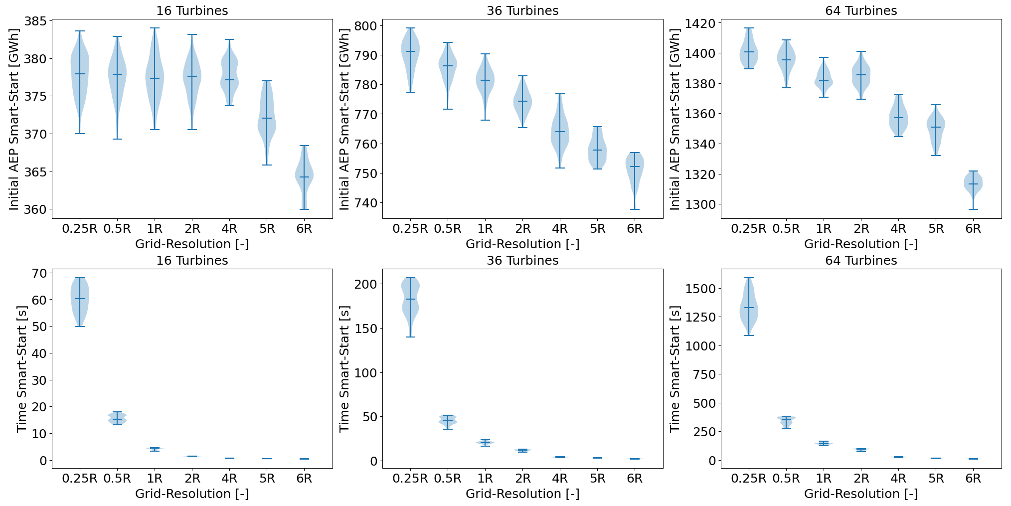
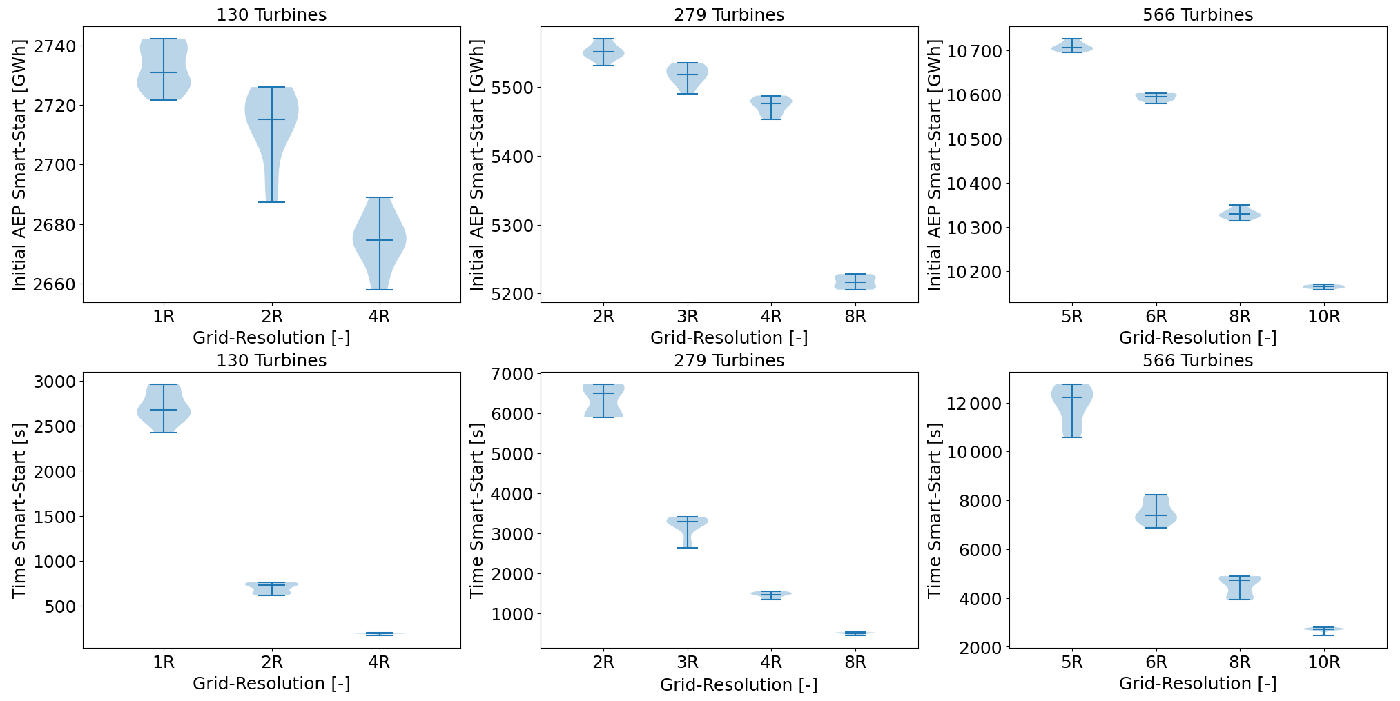
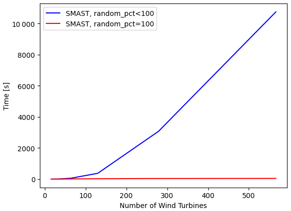
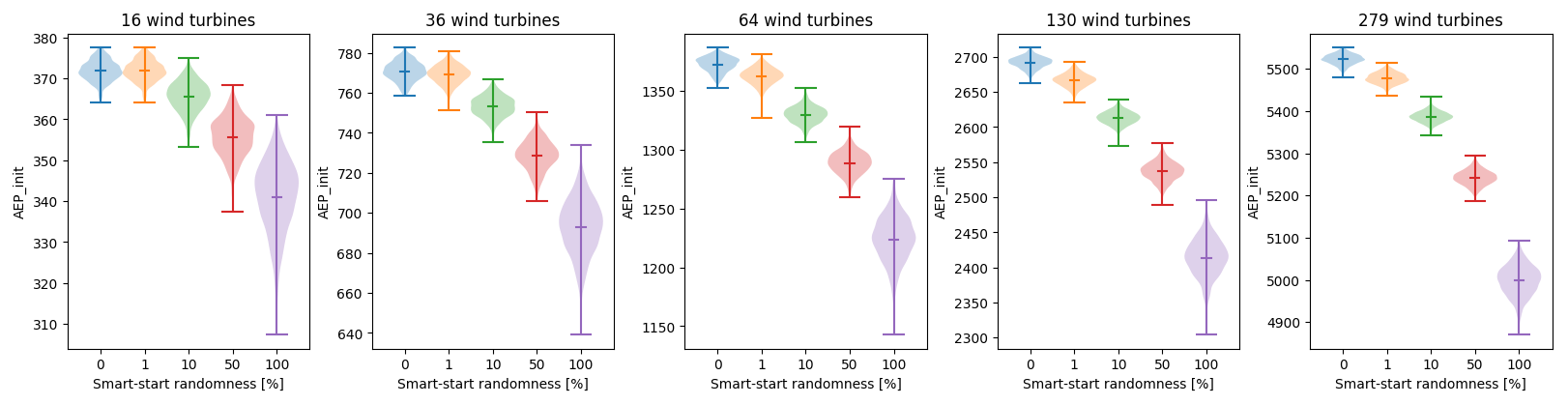
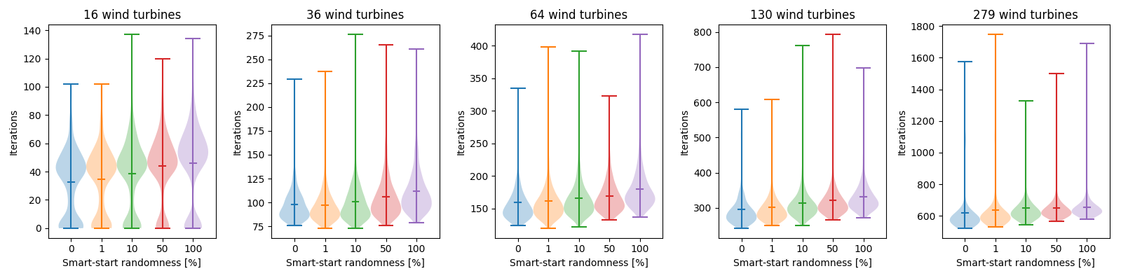
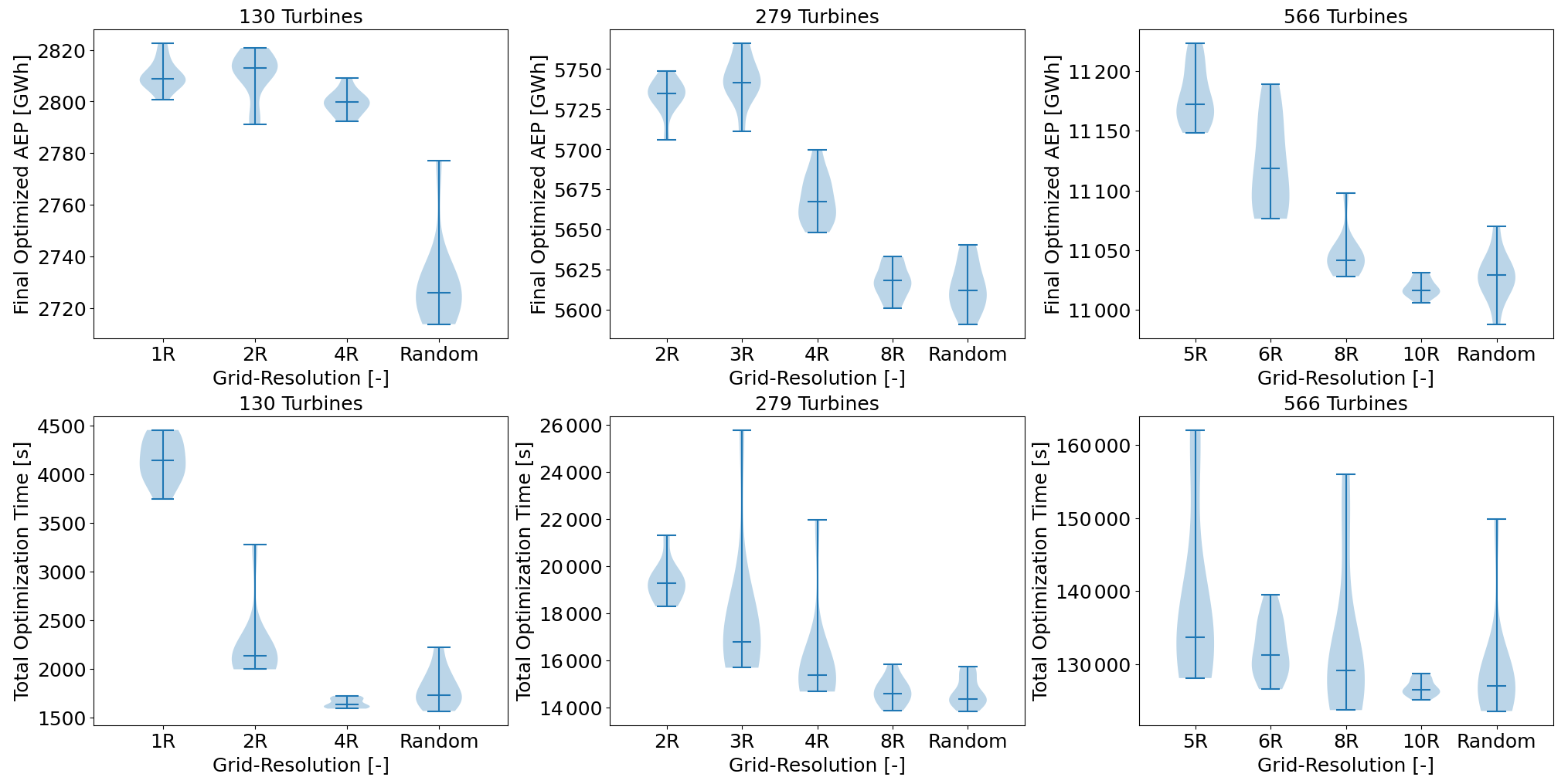
Figure F1 Final AEP and optimization time of SMAST as compared to randomly generated layouts.