the Creative Commons Attribution 4.0 License.
the Creative Commons Attribution 4.0 License.
 | 21 Feb 2024
A novel techno-economical layout optimization tool for floating wind farm design
Amalia Ida Hietanen
Thor Heine Snedker
Ilmas Bayati
Over the past few years, the offshore wind sector has been subject to renewed yet growing interest from the industry and from the research sphere, with a particular focus on a recently developed concept, the floating offshore wind (FOW). Because of its novelty, floating research material is found in limited quantity. This paper focuses on the layout optimization of a floating offshore wind farm (FOWF) considering multiple parameters and engineering constraints, combining floating-specific parameters together with economic indicators. Today’s common wind farm layout optimization codes do not take into account either floating-specific technical parameters (anchors, mooring lines, inter-array cables (IACs), etc.) or non-technical parameters (operational expenditure, OPEX; capital expenditure, CAPEX; and other techno-economic project parameters). In this paper, a multi-parametric objective function is used in the optimization of the layout of a FOWF, combining the annual energy production (AEP) together with the costs that depend on the layout. The mooring system and the collection system including the inter-array cables and the offshore substation are identified as layout-dependent and therefore modeled in the optimization loop. Using ScotWind site 10 as a study case, it was found with the predefined technical and economic assumptions that the profit was increased by EUR 34.5 million compared to a grid-based layout. The main drivers were identified to be the AEP, followed by the anchors and the availability associated with the failures of inter-array cables.
- Article
(7137 KB) - Full-text XML
- BibTeX
- EndNote


Today, offshore wind farms are located for the most part in shallow water areas, where it is possible to install bottom-fixed offshore wind turbines (BOWTs). Monopiles remain the preferred foundation choice of developers with over 80 % of all installations in 2020, with jacket structures coming in second with 10 % of the installations (Ramírez et al., 2020). While the first full-scale FOWF was installed in 2017 off the coast of Scotland, FOW still appears as the next frontier to cross in the wind industry. Nevertheless, floating offshore wind turbines (FOWTs) come with a state-of-the-art technology that allows us to exploit areas with a water depth above 60 m, which is unfeasible for BOWTs. Indeed, FOWTs differ from BOWTs as they are not fixed to the seabed on a foundation but attached with a mooring system. Hence, FOW appears as a solution to harness the full potential of offshore wind while reducing the constraints in terms of water depths and soil conditions.
However, to be economically competitive with bottom-fixed offshore wind farms (BOWFs), the costs of FOWF projects need to be minimized to make them more attractive for developers and investors. Due to their complex and novel technology, FOWTs have higher installation, maintenance and decommissioning costs than BOWTs. The main reason for that is the limited site accessibility because of possible incompatible weather conditions, expensive installation procedures and high grid connection costs. The capital expenditure (CAPEX) of FOWTs ends up being about twice the CAPEX of BOWTs (Maienza et al., 2020). FOW cost reduction is therefore an area that needs to be investigated – for example, through layout optimization, which is the focus of this project.
In the literature, wind farm layout optimization is, for the most part, applied to BOWFs, first introduced by Mosetti et al. (1994) using a genetic algorithm and then by others (Lackner and Elkinton, 2007; Charhouni et al., 2019; Rodrigues et al., 2016; Pillai et al., 2017). The most common objective function found in the literature is the annual energy production (AEP) considering wake losses (Charhouni et al., 2019; Rodrigues et al., 2016; Froese et al., 2022). This approach is used to obtain the optimal layout that leads to the highest production, but it does not take into account any cost consideration. Tesauro et al. (2012) investigated the relevance of objective functions in wind farm layout optimization. While the mere formulation of the objective as AEP was proven to be reductive since it leads to layouts where the wind resource is the highest without considering the cost of foundations, of the vessels for installation, of the connection cables and so on, the net present value (NPV) and the financial balance were found to be more relevant for wind farm layout optimization. As for floating wind layout optimization, Froese et al. (2022) are some of the first researchers to include floating-specific parameters in the optimization loop. They optimized the layout of a wind farm while optimizing the design of the mooring system at the same time, with the AEP as the objective.
In the present paper, the layout of a wind farm will be optimized using the NPV as the objective function, while optimizing the inter-array cable routing and modeling floating-specific components (anchors, mooring lines, dynamic cables) and constraints.
2.1 Problem formulation
In this section, the FOWF layout optimization framework is presented. The problem takes the form of a multi-constrained and multi-parametric maximization problem as given in Eq. (1).
where ω stands for the different decision variables, Ω is the set of constraints applied to ω and 𝕁 is the cost function which derives from the project's relative NPV.
2.1.1 Assumptions
Below, a list of the assumptions considered in the problem is given.
-
The number of FOWTs in the wind farm is fixed to N.
-
All FOWTs are assumed to be identical, meaning that the rotor diameter, the hub height, the rated power, and the cut-in and cut-out wind speeds are the same across the whole wind farm.
-
The area 𝒜 of the wind farm is fixed, and real wind resource and seabed data specific to the chosen site are used in the modeling.
-
A uniform sea depth zdepth is calculated as the average depth of the site area 𝒜.
-
The wind resource is spatially uniform.
2.1.2 Decision variables
The set of design variables of the framework is chosen to be the coordinates of the FOWT centroids, as presented in Eq. 2.
2.1.3 Constraints
The design variables are subject to engineering and operational constraints, defined in Eq. (3).
In the first constraint, it is necessary to make sure that all components of the FOWTs are inside of the area 𝒜, especially in the case of floating. In traditional layout optimization problems, the wind turbines are BOWTs, which does not require much more than constraining the centroids of the BOWTs in the site area. In this project, to account for the anchors and mooring lines, a buffer zone that reduces the site by the footprint of the mooring lines is constructed. Therefore, the area 𝒜 is defined as the area inside of the buffer zone.
The mooring distance constraint allows us to give more freedom in the layout design. Indeed, if a circular distance constraint is considered to account for the mooring lines, then it reduces the layout possibilities in comparison to the constraint chosen in this project, where the mooring lines can overlap while respecting a limit distance as it is shown in Fig. 1.
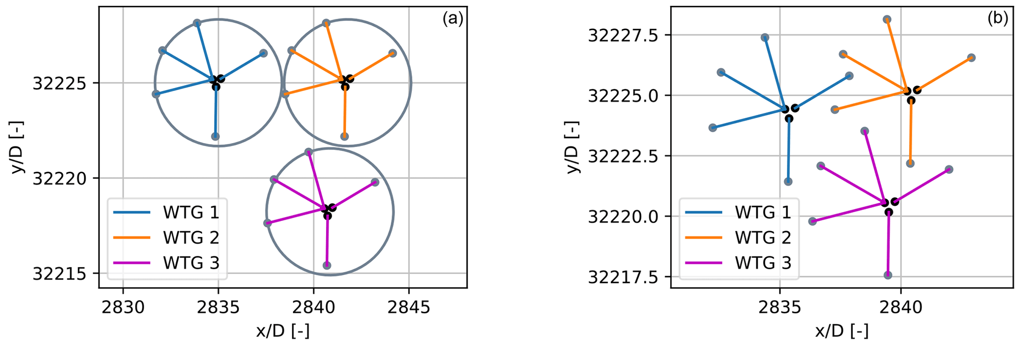
Figure 1Possible layouts for three turbines using the circular constraint where the mooring lines are constrained in circles (a) and geometrical constraint where the mooring lines can be overlapping (b)
The two distance constraints could in theory be combined because if the mooring distance constraint is satisfied then the centroid distance would be satisfied as well. However, using only the constraint on the mooring lines, though it is directly related to the set of coordinates , it can lead to a scenario within the optimization where two turbines are at the exact same position. The latter would lead to an error and the optimization would break. dmin is therefore the very minimal distance that two turbines can be separated by, i.e., the footprint length of one mooring line.
2.1.4 Objective function
The objective function chosen in this project derives from the NPV, which is the total profit of the wind farm through its lifetime, converted to present-day value. It is a scalar-valued cost function that includes the AEP, the price of electricity pkW h, the operational expenditure (OPEX) and the CAPEX. It only includes the components Comp(X) that depend on the turbine positions and not the fixed cost components Compfixed. As it has been stated by Tesauro et al. (2012), the costs that are not influenced by the actual wind farm layout (cost of planning, cost of the civil infrastructure, price of the electrical connection to the main grid, etc.) are considered irrelevant and not modeled in the project framework. These fixed costs can be added as a post-processing calculation, as they are not related to the layout.
The objective function used in the project is given in Eq. (4).
where AEP(xi, yi) is the annual energy production including layout-variable losses, pkW h is the price of electricity, OPEX(xi, yi) and CAPEX(xi, yi) are the layout-variable components of the OPEX and of the CAPEX respectively, and a is an annuity factor defined in Eq. (5).
where r is the interest rate and ny the lifetime of the wind farm.
In this project, the NPV was preferred over the levelized cost of energy (LCOE) because the LCOE has the drawback of increasing, i.e., getting worse, as the size of the wind farm increases. On the other hand, the total profit of a project would typically increase with the size of the wind farm (EMD, 2022). On top of that, the time dependency of the price of electricity and of the OPEX in the NPV can later be included in the optimization tool to assess of the evolution of the NPV over the lifetime of the FOWF. That being said, both the LCOE and the NPV are relevant to use in an optimization framework, as they both have their own advantages and drawbacks.
2.2 Summary of the techno-economic modeling
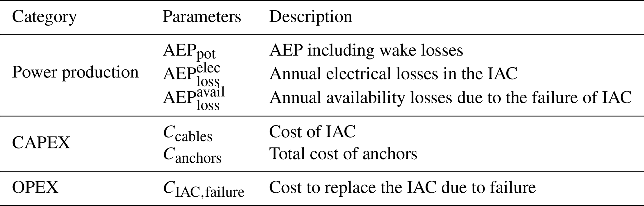
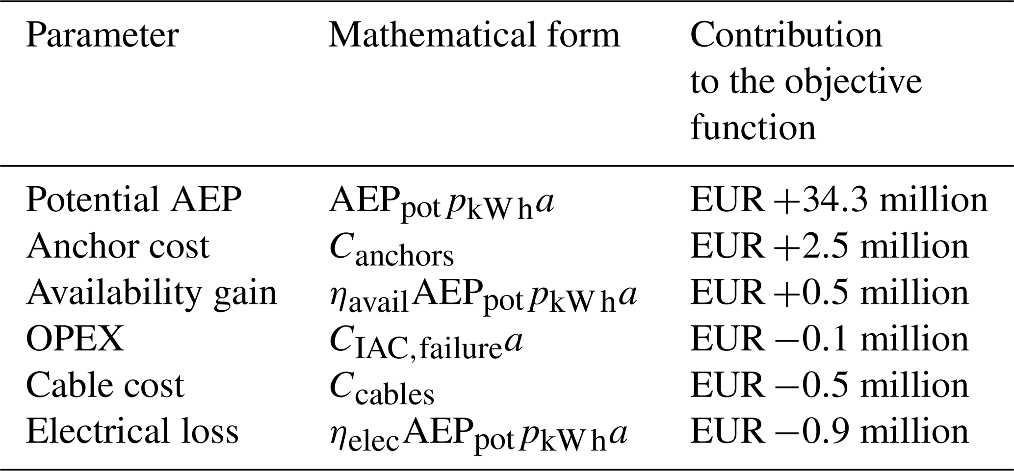
Therefore, the final objective function is summarized in Eq. (6). The components of the objective function that were identified as relevant in the modeling of the optimization problem are summarized in Table 1.
where ηtot is the efficiency of the layout-variable production losses defined in Eq. (7) and AEPpot the potential AEP. The latter is computed using the Python library PyWake by Pedersen et al. (2023) using Bastankhah and Porté-Agel wake model (sum of all wind turbines, directions and speeds). The potential impact of the floating technology is not included in the AEP computation.
In Eq. (7), the total annual electrical and availability losses are computed as shown in Eq. (8), with and defined in Eqs. (14) and (15). T represents the number of hours per year.
2.3 Optimization algorithm
In this work, a gradient-free heuristic optimizer based on a random-search algorithm by Feng and Shen (2015) is used. This algorithm was developed in Python within the package TopFarm – based on the OpenMDAO library. The random-search algorithm starts from an initial feasible layout and then improves it iteratively. The optimization process follows the steps described below.
-
Random move. The algorithm selects one wind turbine generator (WTG) randomly and then moves it randomly.
-
Feasibility. If the design variables do not satisfy the constraints, the algorithm goes back to step 1, until the constraints are satisfied.
-
Evaluation. The objective function is computed once a feasible layout is found.
-
Update. If the objective function is improved, the algorithm goes back to step 1 and moves the previously moved WTG. Else, it also goes back to step 1 but chooses a random WTG to move.
The algorithm includes some adaptive mechanisms, meaning that the information of a good move is recorded and utilized later for the next random moves, as described in step 4.
A random-search algorithm was chosen over a gradient-based algorithm because it allows us to move out of the local optima. Gradient-based optimization algorithms tend to quickly converge towards local optima, especially when the initial layout is close to a local optima. On the contrary, random search presents the advantage of never getting stuck in local optima since the positions of the turbines are moved randomly. To make sure that the random search provides the best solution, simulations can be run several times to obtain a distribution of the optimal results.
2.4 Modeling of floating-specific components
2.4.1 Floating platform
The floating platform is modeled using the geometry of a semi-submersible floating platform, with five mooring lines. The floating platform orientation ϕ – which also drives the orientation of the mooring lines – is aligned to the main wave direction to maximize the stability of the structure.
2.4.2 Mooring lines
The mooring lines are attached to the fair leads of the floater, positioned at each of the corners of the platform. They are then anchored to the seabed. The mooring system gives some freedom to the FOWTs to move their positions laterally through surge and sway motions. Following in the steps of the oil and gas industry, FOWTs platforms are designed together with their mooring system in order to reduce the lateral displacements (Mahfouz et al., 2022). The floating platform in this project has an asymmetric mooring system (three mooring lines in the “left” part and two mooring lines in the “right” part of the platform), which means that the FOWTs will have different distances relative to each other for each wind direction. Therefore, to avoid collision and friction and to facilitate operations, the mooring lines must be separated by a certain distance, and most importantly the mooring lines are not allowed to cross.
Therefore, a distance constraint between the mooring lines is implemented to avoid this problem. This constraint is included within the optimizer by calculating at each iteration the distances between the different mooring lines of each turbine. A distance matrix sized N×nmooring is computed – with nmooring the number of mooring lines per FOWT – and if the minimum value of this matrix is greater than the distance constraint, then the distance constraint for mooring lines is satisfied and the layout can be retained. To reduce the computational effort, the strictly upper triangular matrix only is computed since the distance matrix is symmetrical and has zeros on its diagonal.
Acknowledging the potential for displacements in the mooring system, this study intentionally omits the consideration of its dynamic behavior in the model to streamline the optimization process.
2.4.3 Anchors
According to Lieng et al. (2022), manufacturing and installing anchoring systems is a major cost driver of a FOWF. The cost of anchors depends on the required holding power and weight, which are driven by the seafloor technical conditions. For instance, it is easier to install an anchor in sand than in bedrock (DTOcean, 2015).
Different types of anchors exist in the industry: drag-embedded, driven piles, suction piles, gravity anchors, etc. In this paper, two types of anchors are considered: drag anchors for cohesive sediments (e.g., sand-based seabed) and driven anchors – applicable to a wide range of seabed conditions but much more difficult and expensive to install and difficult to remove upon decommissioning (Ros and James, 2015). In the design of the wind farm, the idea is to use an optimal – but not necessarily minimal – number of drilled anchors to reduce costs, installation risks and environmental impacts.
To do so, a map of the seabed bedrock depth is included in the optimization. The zones where the bedrock is more than 5 m under the sand are defined as suitable for drag anchors, while the rest of the area needs drilled pile anchors. Therefore, a binary map is created as shown in Fig. 2, where the blue zones are sand-prevailing and the red zones are bedrock-prevailing. Eventually, the idea is to compute the positions of the anchors at each iteration in the optimizer and to compute the associated costs according to the type of seabed where the anchors fall. Further, this anchor cost component is included in the objective function, and the optimizer evaluates how valuable it is to move a FOWT from a bedrock-prevailing zone to a sand-prevailing zone, according to its contribution to the overall costs.
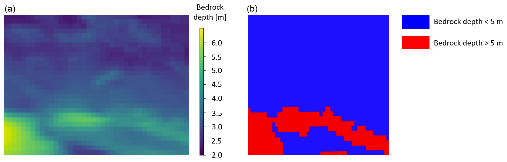
Figure 2Non-binarized (a) and binarized (b) maps of the bedrock depth under the seafloor. These map do not showcase the water depth – they only show how deep the bedrock is under the seabed.
In the model, it is possible to mix the kinds of anchors on a FOWT, meaning that a given FOWT can have both drilled anchors and drag-embedded anchors.
2.4.4 Dynamic cables
Inter-array cables are modeled and optimized in a sub-optimization routine that minimizes the total cable length inside of the main optimization loop. The umbilical dynamic cable section is modeled as well to adjust the total inter-array cable length. Further, the electrical losses together with the availability losses due to cable failure are computed to correct the AEP.
-
Cable routing. The collection grid, and especially the inter-array cable layout, is highly dependent on the wind farm layout. Not only does it affect the costs but it also plays a key role in the energy yield. It is therefore relevant to include the cable-routing design in the optimization loop to evaluate its influence on the overall costs. To maximize the efficiency of the whole optimization, the cable layout is optimized by a sub-optimization algorithm at each iteration of the main optimizer.
The cable-routing optimization is based on the Esau–Williams heuristic algorithm and was developed by Souza de Alencar (2022). The objective function of the algorithm is to minimize the total cable length. The algorithm finds sub-optimal solutions that are very close to the exact solutions. This algorithm has a very good performance and accuracy with a low computational effort, which is crucial here since an optimized cable layout needs to be computed at each iteration of the main optimization. Because the optimization already has a great complexity with multiple constraints and parameters, the cable optimization is kept simple. The Esau–Williams heuristic is built using a minimal-cost spanning tree of a graph, with designated roots, nodes and capacity constraints. In this paper, the roots of the spanning tree are the offshore substation(s) (OSS), while the nodes are the FOWTs. The algorithm allows sub-branches on a given string, while respecting a maximum number of nodes per string. An example of an optimized cable routing is provided below in Fig. 3.
Two constraints are defined in the cable sub-optimization algorithm:
-
non-crossing constraint, which prevents two IAC from crossing, and
-
capacity constraint, which determines a maximum number of nodes per string. For cable layouts, this capacity constraint is defined by κ, i.e., the maximum number of turbines per cable string, which is computed in Eq. (9).
where Pcapacity is the capacity of the IAC used and Prated is the rated power of a turbine.
The power capacity of a cable is defined by the core size of the cable. In practice, inter-array cable layouts have two or three core sizes with smaller sizes at the end of the strings to reduce the costs. In this project, to simplify the process, a single core size is used.
-
-
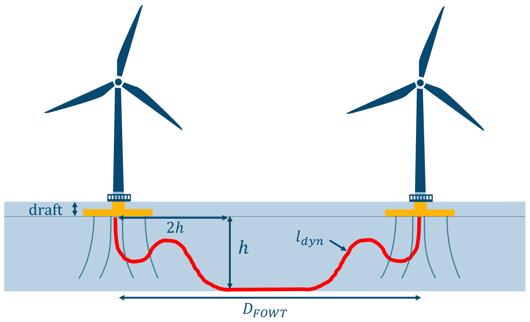
Dynamic section. While BOWTs' inter-array cables are installed buried or secured on the seabed, FOWTs' inter-array cables have a dynamic section that enables them to move together with the floating platform. Dynamic sections can be either in catenary shapes or in lazy-wave umbilical shape. It was shown by Rentschler (2020) that the catenary shape is not suited for water depths above 100 m, while umbilical shapes can be used in water depths of more than 200 m. On top of that, catenary shapes are more susceptible to platform movements than umbilical shapes and are therefore prone to higher compression and fatigue at the touchdown point. On the other side, umbilical shapes decouple the platform and cable movement, which makes them preferable over catenary shapes.
The cable is fixed at a certain distance from the water surface, corresponding to the draft of the floating platform. The hang-off over the seabed h is given by Eq. (10). The horizontal distance of the cable's fixation point on the seabed is set to 2 h, as recommended by Rentschler (2019).
Rentschler (2019) found a general design rule, which is that there is a constant ratio between the total length of the dynamic cable ldyn and h, as written in Eq. (11). This is retained as a general formula to compute the length of the inter-array cables.
Eventually, the total cable length Ltot between two entities is computed following Eq. (12) (Lerch et al., 2021).
where DFOWTs is the horizontal distance between the two turbines (or turbines–OSS) connected together, ldyn is the dynamic section length and 2h is the horizontal distance from the two cable fixation points.
-
Offshore substation. The OSS transmits the power from all the FOWTs to the shore transmission network through an export cable towards an onshore substation (OnSS). In this paper, the number of OSSs and their positions are fixed, so the length of the export cable(s) and the associated losses are fixed. Therefore, the costs associated with the OSS, with the export cables and with the OnSS are not included in the optimization loop. Since the OSSs in a FOWF are also generally mounted on floating structures, the dynamic cable sections of the cables connected to the OSS are computed as written in Eq. (11) and added to the total cable length in Eq. (12).
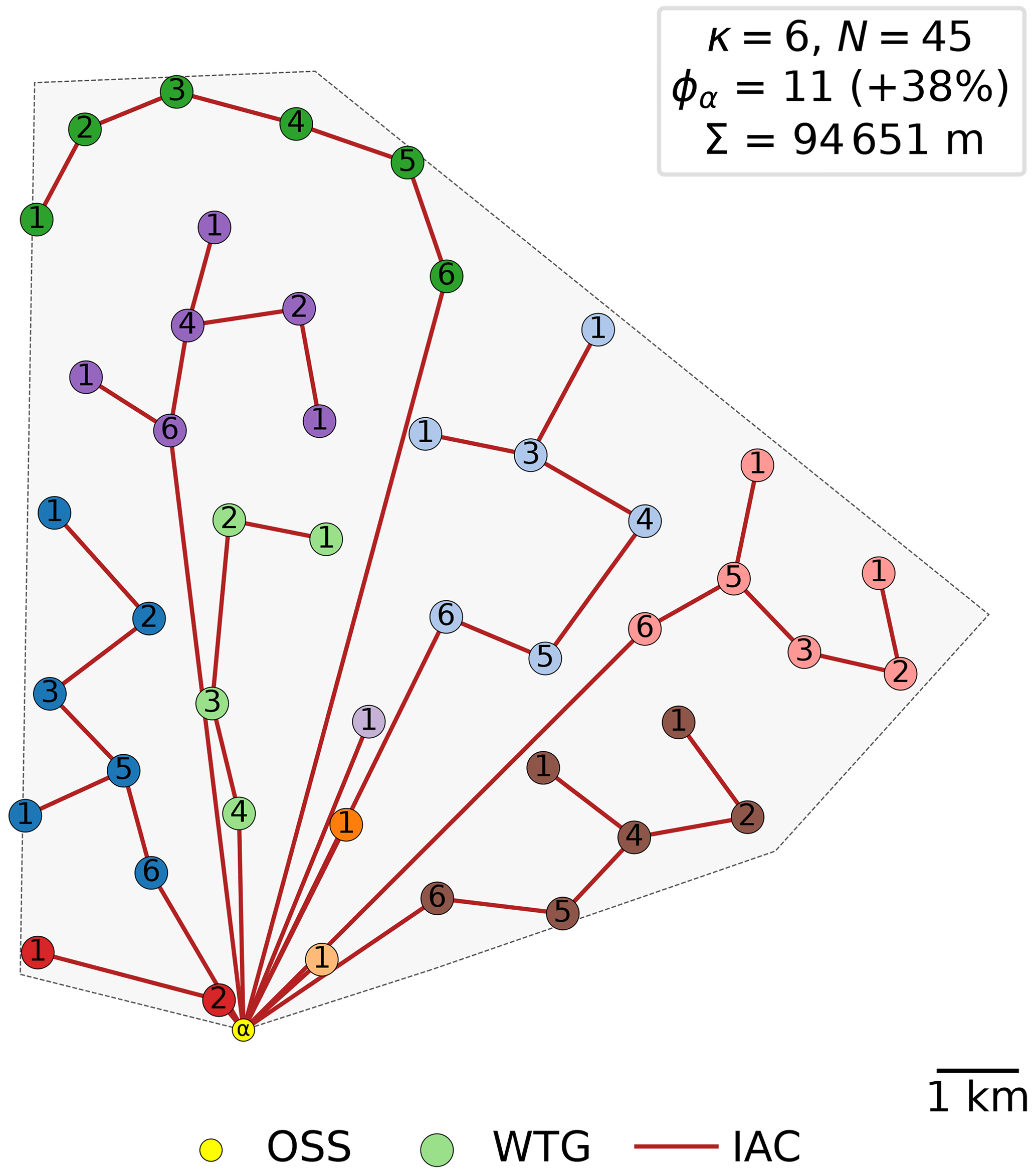
Figure 3Optimized cable routing with one OSS and a max of six FOWTs per cable string (κ=6). N is the number of turbines, Φa is the total number of cable strings and Σ is the horizontal cable length.
2.4.5 Electrical losses
For the cable section Si, the power loss is given by Eq. (13).
where is the power generated by FOWTi at the end of the cable Si, is the power transmitted to FOWTi, U is the voltage applied, is the resistance of cable Si and is the length of cable Si.
The power losses are computed starting from the end of a cable string where no power is transmitted from a downstream turbine, and then the losses are computed at each upstream FOWT until the OSS is reached. Eventually, the final power losses are given by Eq. (14).
where nOSS is the number of OSSs and is the power transmitted to the OSS.
While the electrical power loss is linearly linked to the length of the cable, it is proportional to the square of the power going through the cable. The power loss is also closely linked to the cable layout and especially
-
the number of cable strings in the cable layout,
-
the number of turbines per cable string and
-
the length of the cable sections.
From an analysis carried out in this study on the cable-routing subroutine – using a wind farm with an AEP of 2550 GW h and with 45 FOWTs – it is shown in Fig. 5 that the number of cable strings drives the electrical losses. If all turbines are connected on a single string, then the production loss explodes and reaches over 6 % of the AEP, while if the layout contains more strings, the production loss drops. With 45 cable strings, the electrical loss is below 0.2 %. However, the length of the cables increases with the number of cable strings. Therefore, it is important to combine the production together with its losses and the material costs to find a balance and reach the optimum in the optimization phase.
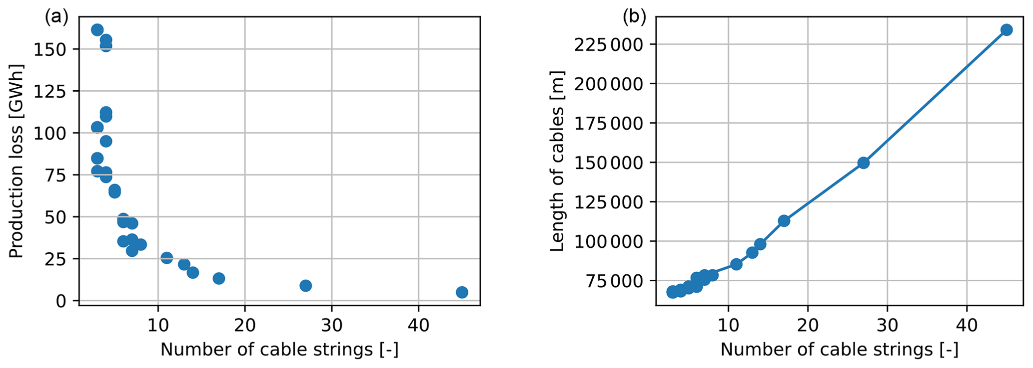
Figure 5Number of cable strings as a function of the cable length (a) and annual electrical losses as a function of the number of cable strings (b).
Figure 5 is obtained from the Esau–Williams heuristic cable optimization. The number of cable strings is computed internally within the optimizer. The only input here is the maximum number of turbines per string, which affects the number of strings. This is the reason why there are gaps between and ; the optimizer creates strings of one FOWT, then strings of two FOWTs and so on. However, even if it is allowed to create strings of two FOWTs, the solver can find a better solution with only one FOWT on a string. For example, the point at nstrings=27 corresponds to 18 strings of two FOWTs and 9 strings of one FOWT (see Fig. 6). In this example, two OSSs were chosen to separate the layout into two groups and facilitate the readability. The number of OSSs does not affect the results described above as the losses that occur in the OSS are not accounted for. Later, one OSS only is chosen due to the relatively low number of turbines of the chosen site.
2.4.6 Availability losses
When it comes to wind farm layout optimization, the availability of the IACs comes as a layout-variable loss. Indeed, according to the cable layout, and especially how the turbines are organized in the cable routing (number of strings, number of turbines per string, etc.), a cable failure can potentially disrupt global production to a greater or lesser extent.
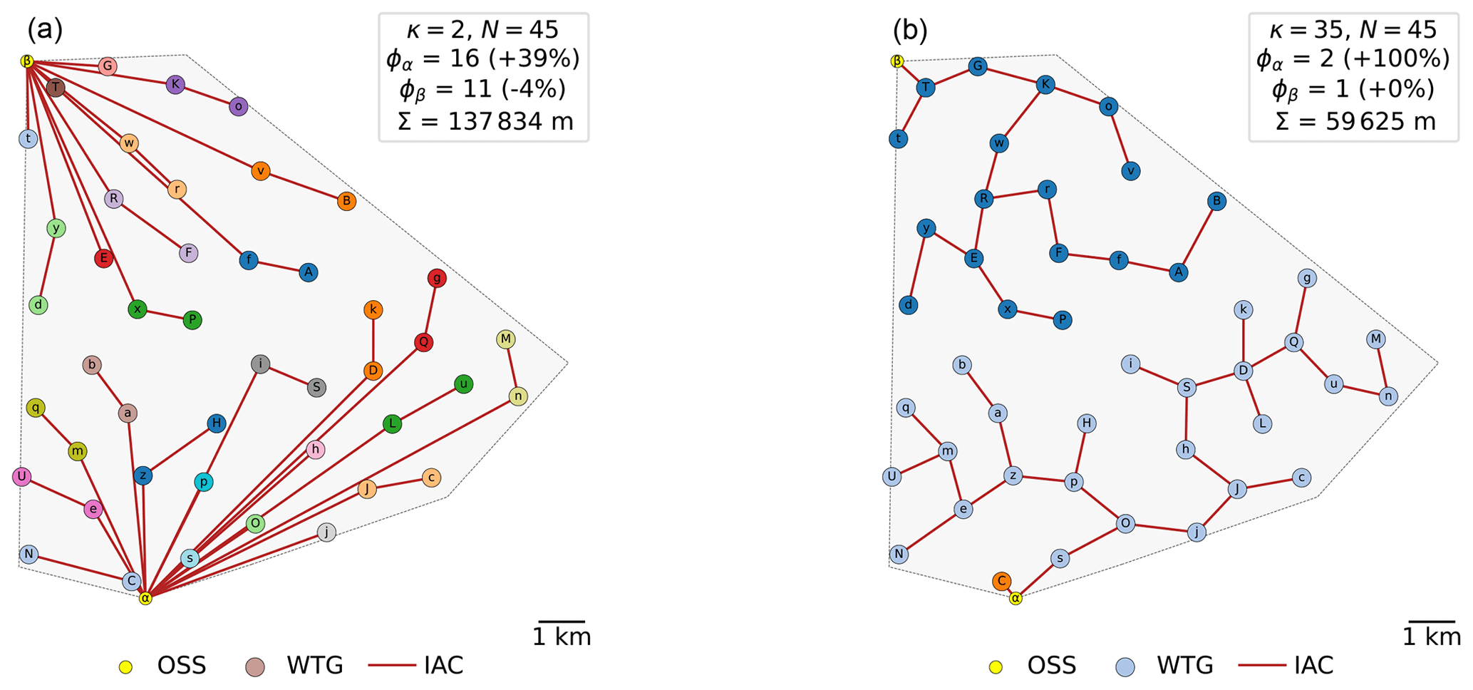
For example, Fig. 6 shows two cable routings, with a maximum of two FOWTs per string (left) and a maximum of 35 FOWTs per string (right). In the first case, on average, the production of 1.4 FOWTs is affected by a cable failure. In the second case, on average, the production of 5.8 FOWTs is affected by a cable failure.
To compute the availability losses, for each cable section, the power produced by the turbine at the end of the cable section together with the power produced from the downstream turbines are computed. Eventually, the losses triggered by a failure of each of the cable sections are computed following Eq. (15).
where FRi is the failure rate of the cable Si.
The failure rate for each of the cable section is computed following the research from Zhang et al. (2019), where they have investigated the failure rate of submarine cables and found that the failure rate is a function of the cable length. Their findings are adjusted to be compliant with dynamic cables as shown in Eq. (16) using assumptions from Lerch et al. (2021).
Using the failure rate of each of the cable sections, the cost to replace the cables in case of failure can be computed, as shown in Eq. (17). This cost is an OPEX component; it represents the yearly cost of cable failures.
where CIAC is the cost of IAC per unit length.
Scotland has a long history of developing floating systems starting with oil and gas. The expertise in this sector was used as a strong basis to get started in the floating wind sector. Scotland emerges as a global leader in floating wind deployment, with Equinor's 30 MW Hywind Scotland inaugurated in 2017, Kincardine following suit in 2021 and Pentland on track to join the ranks upon completion. On top of these three floating wind farms, in 2022, a total number of 14 floating wind projects have been approved in Scotland through the ScotWind leasing. These projects will benefit the Scottish businesses and community as well as provide a major boost to reach the UK “net zero” state goal (Marcus, 2022). They will also add close to 18 GW of commercial-scale floating wind, making Scotland the largest floating wind market in the world.
3.1 Site under study
In this paper, the site that was chosen to perform the layout optimization on is site 10 from ScotWind projects, which is Broadshore, with a capacity of 500 MW. Broadshore was preferred over the other ScotWind sites due to its relatively small number of turbines compared to the others. Indeed, to test and perform large sensitivity analyses using the optimization with an increased complexity due to the new FOW features, it is necessary to have a reasonable number of design variables, 2N, with N being the number of turbines.
A real study case was chosen to study the relevance and the performance of the techno-economic layout optimization. All inputs are set to be as close as possible to reality so that the optimization is studied under realistic conditions. A detailed list of the inputs is presented in the Appendix A.
On top of the site inputs listed in Appendix A, a bedrock map is required to calculate anchor costs. However, seafloor studies, including measurements of the depth of the seafloor bedrock, are typically carried out by oceanographers or marine geologists using specialized equipment and vessels, which is rather expensive. Therefore, seafloor properties maps are generally not publicly available, and detailed seafloor surveys are carried out only on request, in restrained zones. Hence, a map of the water depth is used instead.
3.2 Results
The optimization of the FOWF layout using the relative NPV as the objective function is run using the assumptions in Sect. 2.1.1 and the inputs in Appendix A. One must note that the result obtained is one of the possible optimal layouts – see Sect. 3.3 for further details.
To report on the performance of the techno-economic layout optimization, the optimized results are compared to the results obtained with a base layout. The base layout has the same properties as the study case, except that the layout is not optimized but designed following a grid pattern.
From Table 2, it is seen that the objective function was increased by 0.8 %, which amounts to EUR 34.3 million. The potential AEP was increased by close to 20 GW h by positioning the FOWTs in locations that reduce the wake effect. The AEP is one of the predominant drivers of the NPV, since the evolution of the AEP has a trend similar to the objective function as shown in Fig. 7.
Table 2Results for the base layout and for the optimized layout.
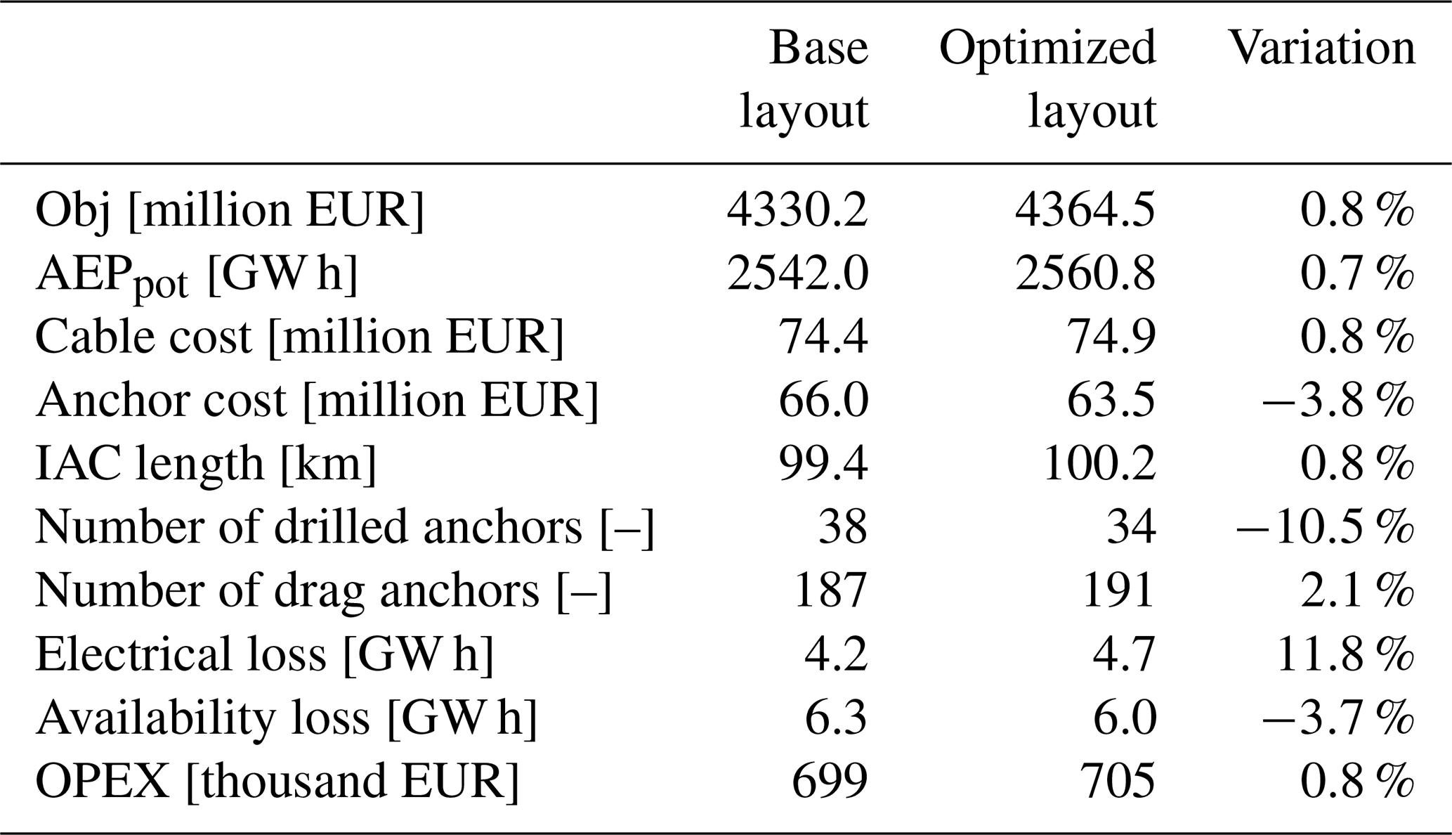
As for the CAPEX elements, the cable cost was slightly increased while the anchor cost was decreased by close to 4 %. In that optimal scenario, the algorithm found that moving the FOWTs out of the bedrock zone provided a higher cost reduction than trying to reduce the IAC length. Indeed, when looking at Fig. 7, the anchor cost shows a descending trend while the cable cost – which is a linear function of the cable length – stays quite stable.
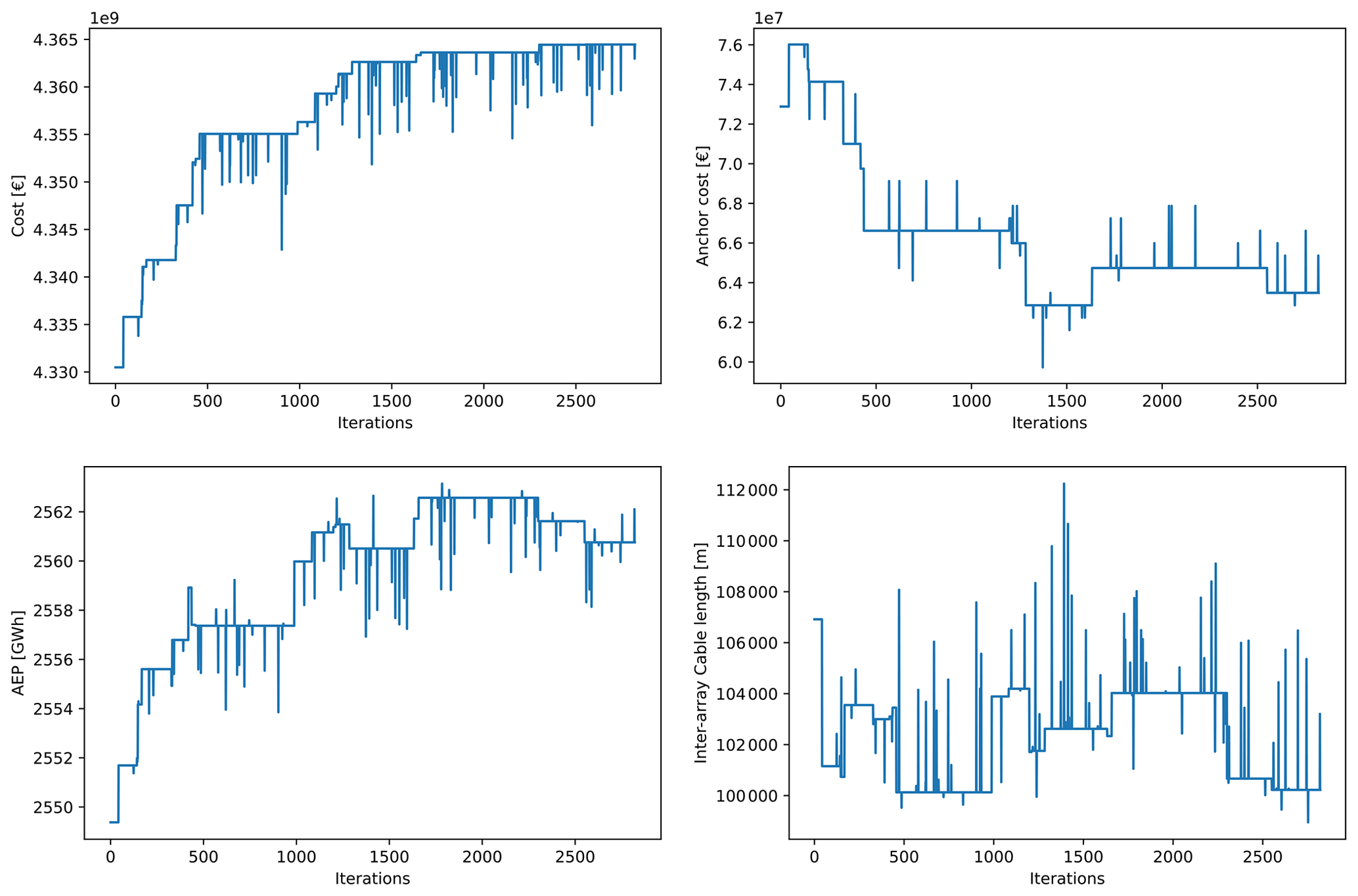
The slight decrease in the potential AEP around iteration 2300 goes together with a decrease in the cable cost and anchor cost. The algorithm ended with a scenario where the potential AEP is not fully maximized, since slightly reducing the CAPEX led to a better relative NPV.
As for the electrical losses and availability losses in Table 2, the electrical losses are slightly increased, because the total IAC length is higher and the production is also higher. However, the availability loss is reduced even though the production is increased. This is due to the combination of the following factors.
-
There are more branches and therefore more turbines with no downstream turbines in the optimized layout than in the base layout, as shown in Fig. 8. The average number of turbines that are shut down due to a cable failure is lower in the optimized layout.
-
The failure rate of each cable section depends on its length.
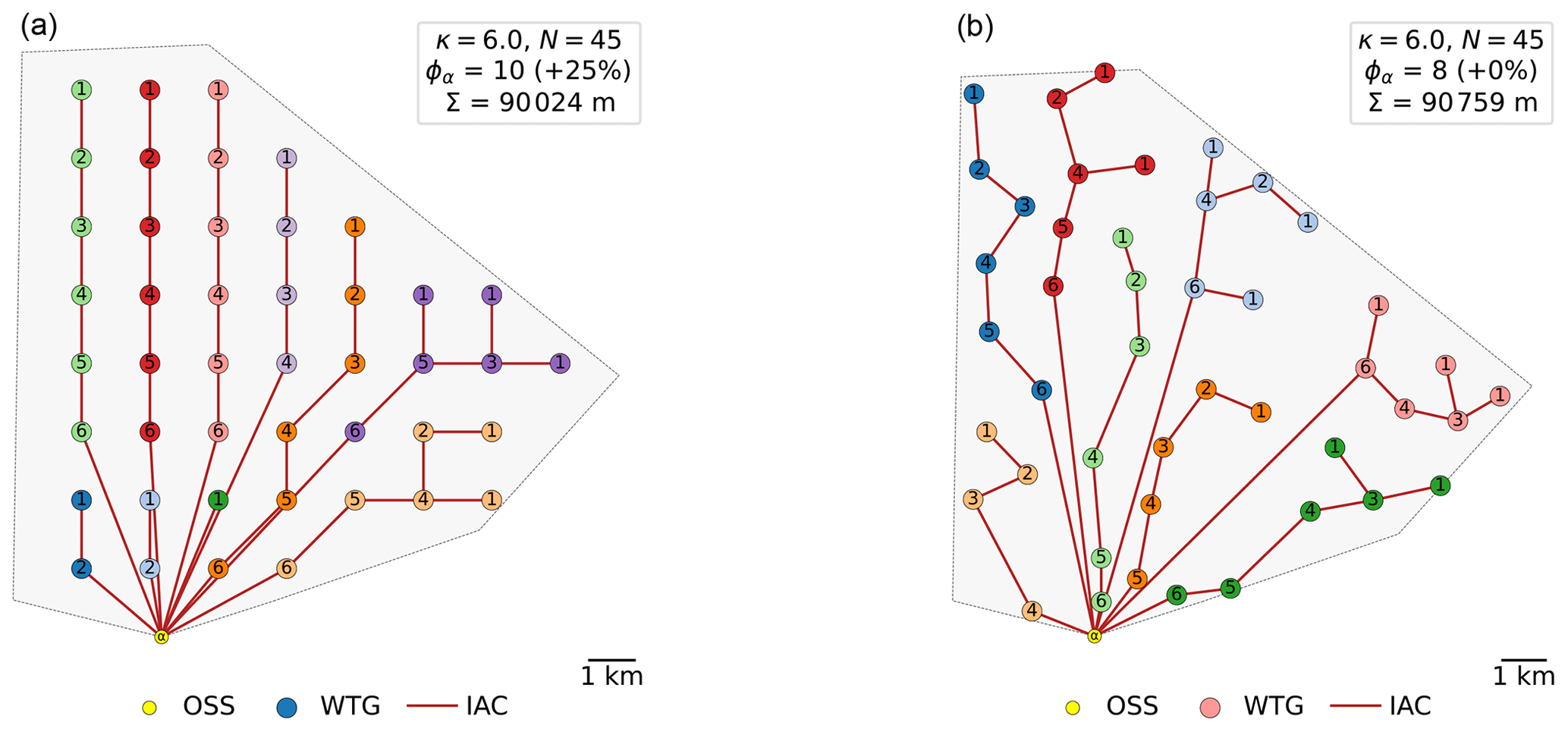
Figure 8Grid-based layout (a) and optimized layout (b) and their associated optimized cable routings for the Broadshore site.
Compared to the base layout, the optimized layout shows that the turbines were moved as much as possible from the bedrock (red) zone, but because the anchor cost is not the only driver of the NPV, some anchors still fall in the bedrock, as shown in Fig. 9.
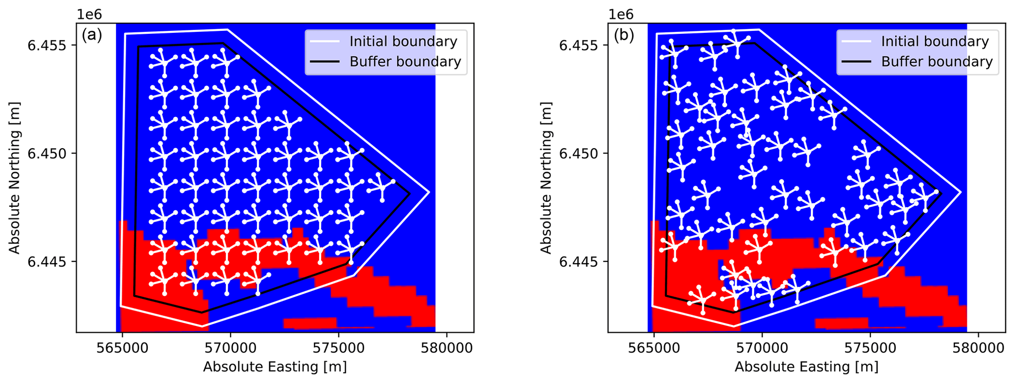
Figure 9Grid-based layout (a) and optimized layout (b) showing WTGs with their mooring lines on the binarized bedrock map for the Broadshore site.
When looking at the base and the optimized layout in Fig. 9 from an aesthetic perspective, the grid-based layout looks more organized while the optimized layout seems to be messy, with the FOWTs' mooring lines overlapping at the bottom of the site. However, the optimized layout satisfies the mooring line distance constraint of 80 m (for the optimized layout the minimum distance between two mooring lines ended up being 81 m, while for the base layout it was 312 m). Even if grid-based layouts are sometimes preferred over irregular ones, optimized layouts bring a non-negligible gain of profit while at the same time satisfying constraints to avoid technical or operational incidents.
To wrap up, it was found with the chosen technical and economic assumptions that the optimized NPV (objective function) was increased by EUR 34.5 million compared to a grid-based layout. The top drivers of the objective function increase are listed in Table 3, with their associated contribution. It is seen that the potential AEP is the main contributor, followed by the cost of anchors and the availability gain. The components of the objective that ended up being “worse” than in the grid-based layout are all related to the cables. It can be said that with the cost assumptions chosen for that study case, the optimization of the AEP and of the anchors is predominant over the IAC optimization.
Table 3Ranking of the drivers of the objective function increase in the multi-parametric optimization.
Additional remarks.
-
The mooring distance constraint defined by was set to 80 m as a project-specific value, but a lower value down to 20 m can be enough for other projects.
-
The grid layout is not optimized. The turbine positions were generated automatically following a grid pattern to match N number of turbines. Here, the grid layout might not be the most optimal grid layout but is only used for comparison purposes.
3.3 Sensitivity analysis
Because economic inputs are subject to a wide range of uncertainties, including changes in technology, energy prices, regulations and consumer behavior, a sensitivity analysis is performed on the most uncertain economic inputs: the electricity price, the anchor costs and the cable cost. Conducting sensitivity analysis allows us to identify how changes in the economic inputs can affect the performance and cost of a wind farm. This information can help to assess the risks associated with different economic scenarios and to identify wind farm layout strategies to mitigate those risks.
3.3.1 Electricity price
In this sensitivity study, a simulation for a given set of parameters is run five times. Figures 10 and 11 show box plots of the distribution of the optimized parameters for different values of the electricity price. As expected, the mean value of the optimized relative NPV grows linearly as the price of electricity increases, because an increased electricity price means more profit, if the other parameters are fixed. Regarding the components of the objective function taken separately, they show a much wider distribution around the median for a given set of parameters than the objective function did. This is because the optimization is based on a multi-parametric objective function, so different combinations of the parameters can lead to the same optimum.

Figure 10Results of the sensitivity analysis on the electricity price – relative NPV and potential AEP.
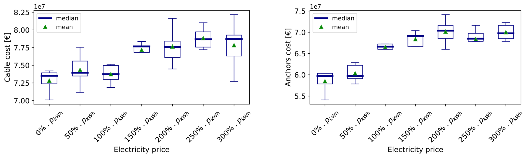
Figure 11Results of the sensitivity analysis on the electricity price – CAPEX components (cable cost and anchor cost).
The AEP evolution in Fig. 10 shows an ascending trend as the price of electricity increases – while the CAPEX component (IACs and anchors) costs get worse (they augment). This is due to the fact that it becomes more and more worth it to move the FOWTs so that the AEP is increased rather than placing them in zones where the associated CAPEX is low. Indeed, with the NPV as the objective function, the performance of the optimization is controlled by the trade-off between costs and AEP, which is defined by the assumed electricity price. On one side, for very high electricity prices, the CAPEX becomes less important and the NPV objective approaches the AEP objective. For very low electricity prices, the AEP loses its importance and the optimization is driven mainly by the CAPEX components.
It is also seen that when the electricity price reaches a certain level – here around 200 %⋅pkW h = EUR 211.2 per gigawatt hour (GW h) – the AEP, the cable cost and the anchor cost seem to reach a threshold. This threshold represents the limit above which it is not possible to increase the AEP anymore – provided that the constraints are satisfied.
When looking closer at the CAPEX components – IAC and anchors – it is seen that for high electricity prices, the distribution of the total cable cost is quite wide, while it is not the case for the anchors' cost. This is due to the fact that the cable length is not only a driver of the CAPEX, but also of the electrical losses applied to the AEP and of the OPEX. This gives the optimizer more liberty, making it possible to reach the same optimal objective function with different cable lengths. Different cable routings that have different total IAC lengths can reach different availability losses/electrical losses, and with a system of compensation, they can reach the same objective function. As for the anchors, they only affect the CAPEX in this model, and their cost is driven by the positions of the FOWTs that make the anchors fall in bedrock zones or in sand zones: high anchor cost means a larger number of drilled anchors – located in bedrock zones – while low anchor cost means a larger number of drag anchors – located in sand zones.
The electrical loss in Fig. 12 shows a quite stable trend, varying by 0.6 GW h, between the maximal computed value and the minimal computed value. With the electrical loss being a function of the production and of the cable length, an ascending curve would have been expected when the price of electricity increases, since both the cable length and the AEP grow as pkW h grows. However, the way the cable routing is designed also drives the electrical losses, and as it has been shown earlier (see Fig. 5), a higher number of strings and branches – and therefore fewer turbines per string – can lead to a lower electrical loss.
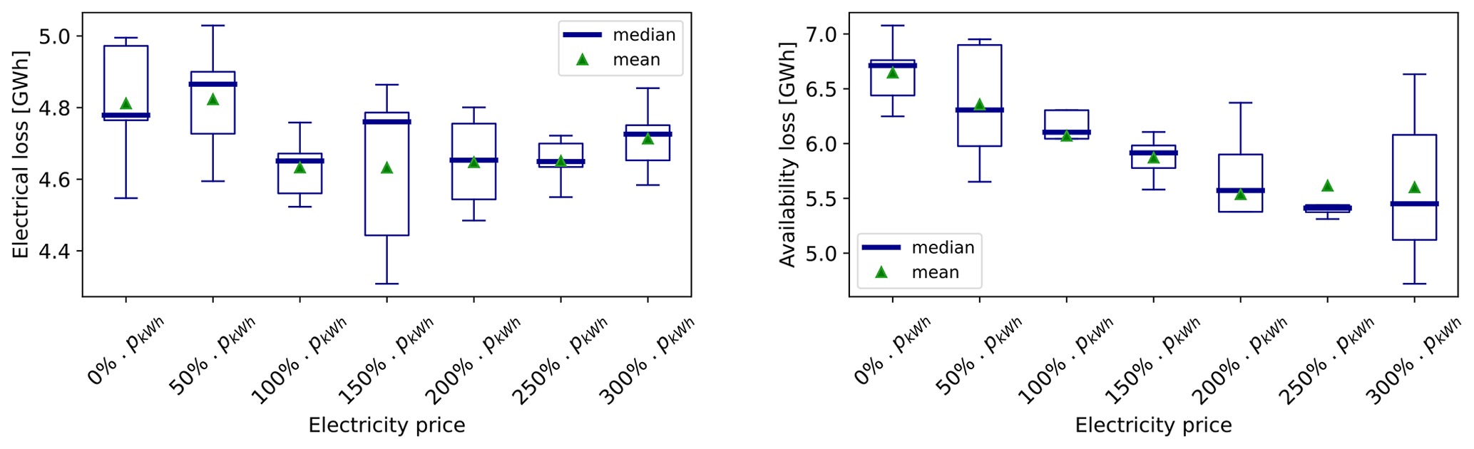
Figure 12Results of the sensitivity analysis on the electricity price – electrical and availability loss.
As for the availability losses, the trend is generally descending as the price of electricity increases, which is related to the cable layout and especially the average load of the wind farm. The average load of the wind farm is defined as the number of turbines connected downstream of a given turbine, averaged across the whole site. In other words, the average load can be seen as the number of turbines affected by the failure of a cable section. In this study, the average load of the wind farm decreases as the price of electricity grows. Therefore, the availability is optimized by playing with the cable-routing design, and it is possible to make it decrease even if the production is increased.
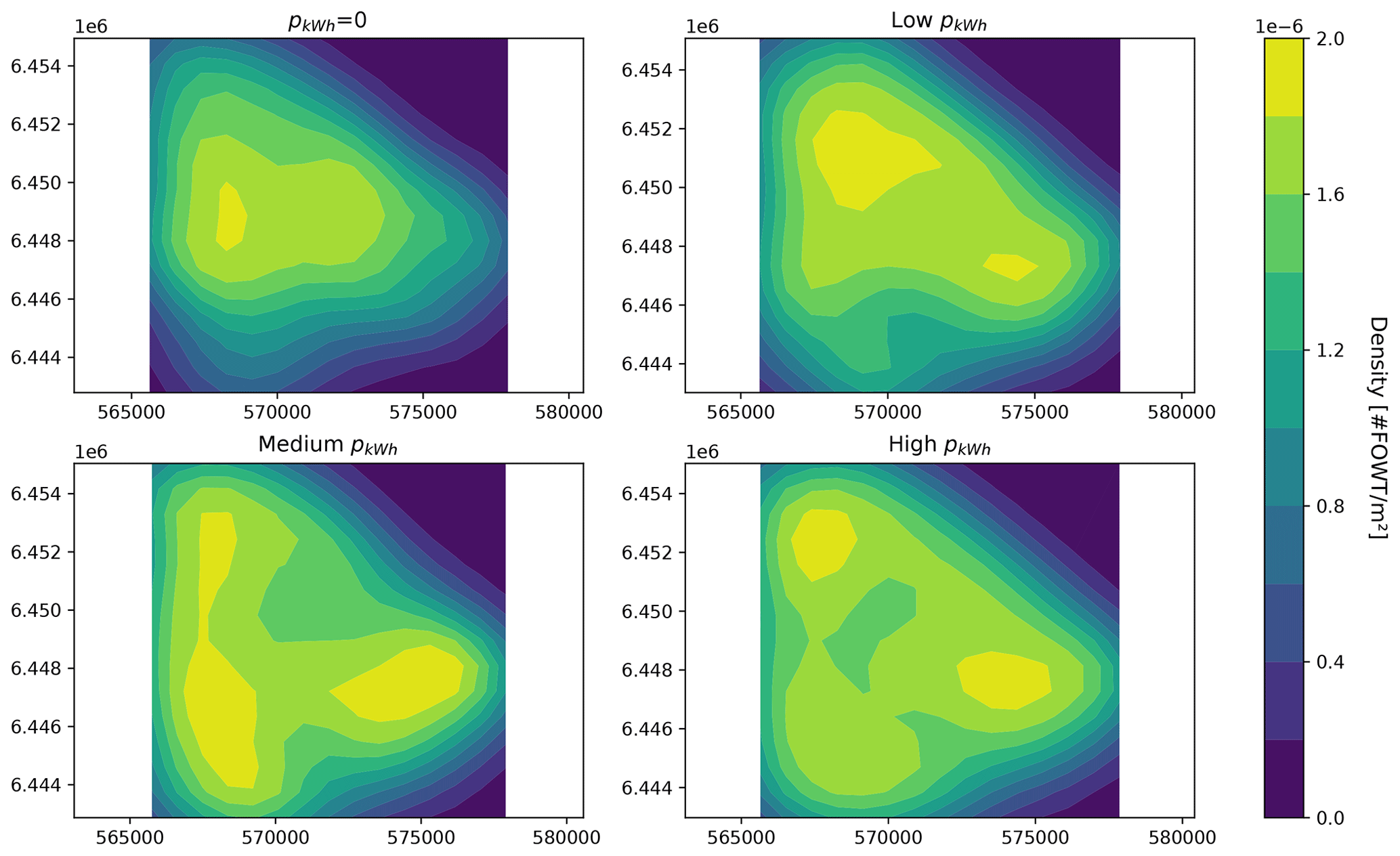
Figure 13Density heat maps of FOWT positions for different electricity price levels; x axis: absolute easting [m]; y axis: absolute northing [m].
To investigate the impact of the electricity price on the optimized layout, a density heat map is generated for different levels of pkW h. It allows us to find out if the optimization process delivers representative layouts with recurring trends in terms of optimal FOWT positions. The heat map is generated by estimating the probability density function (PDF) of the set of optimized coordinates of the FOWTs. It is based on the kernel density estimation (KDE) method, which is a non-parametric way of estimating the PDF of a random variable. In this study, for each electricity price level, five optimal layouts have been generated. The five layouts are merged together and the Gaussian KDE is computed for 0, low (50 % pkW h), medium (100 % pkW h) and high (250 % pkW h) electricity prices, as shown in Fig. 13.
For pkW h=0 in the top left-hand corner of Fig. 13, the optimized layout shows a trend of centering the turbines in the center of the site. In that unrealistic scenario, the AEP is totally neglected, and the anchors and IACs are the only components of the objective function. Therefore, the optimizer gathers the FOWTs together to the south of the site where the OSS is located to reduce as much as possible the IAC cost, but at the same time it avoids the bedrock zone at the south to minimize the anchor cost. For a low price of electricity, then the AEP is taken into account, but it is not predominant, since it is seen that the south bedrock zone is still avoided. As the price of electricity increases, the turbines get positioned more and more evenly all over the site, with a density that tends to converge to a constant density for all locations. Overall, the electricity price affects directly how predominant the AEP is compared to the CAPEX elements and therefore to what extent it is worth it in terms of revenue to spread the turbines across the site to reduce the wake effect.
To assess the variation of the optimized layout compared to the grid-based layout generated in Sect. 3.2, a correlation coefficient between the densities is calculated in Table 4. This is done by correlating the z values of each of the plots in Fig. 13 together with Fig. 14.
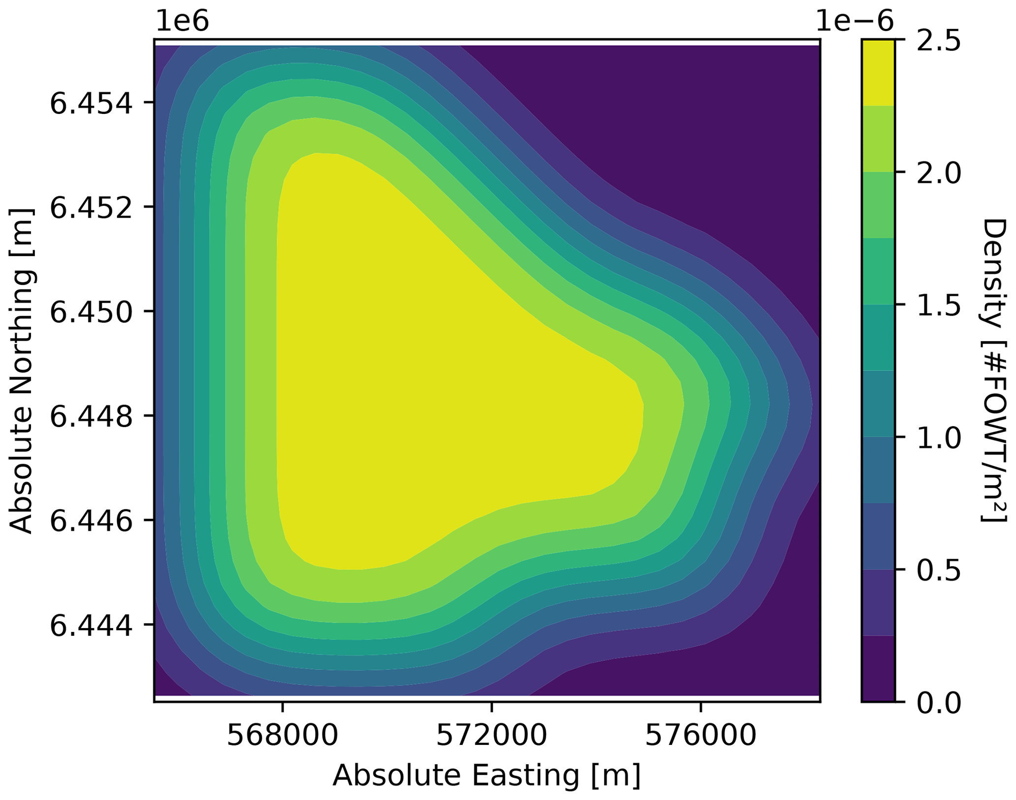
Table 4Table of correlation with the base layout for the electricity price sensitivity analysis.
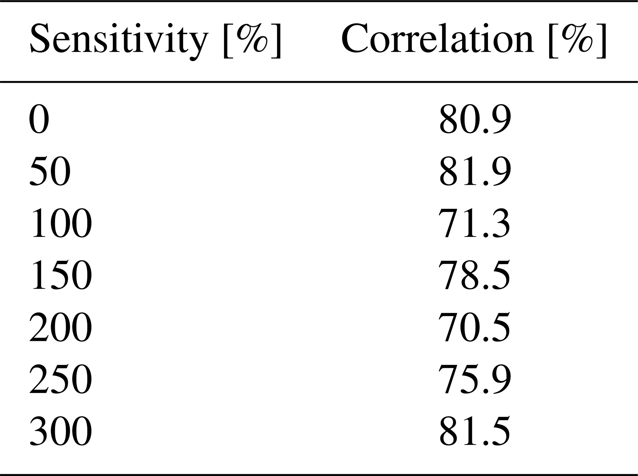
The cases where the electricity price is low have a high correlation coefficient, because the density heat maps show a quite uniform distribution across the site, just like for the grid-based density heat map. Then the case pkW h300 % also has a high correlation coefficient since – as previously mentioned – the turbines are distributed rather evenly on the site, which is similar to the grid-based layout. As for the in-between electricity price values, the correlation is at its lowest because the layouts show an uneven distribution of the FOWTs on the site.
3.3.2 Anchor cost
To stay consistent with the logic of the algorithm – that it is more expensive to install drilled anchors than drag anchors – the cost of the anchors are incremented together:
It is important to determine how the two types of anchors vary from one sensitivity to another and differentiate between them. Indeed, keeping the same difference in cost while making the cost of anchors increase would result in a single scenario, making the increased cost of anchors act as a fixed cost. Here, it is the impact of choosing a type of anchor over another that drives the behavior of the optimization.
In a similar way as stated in the cable cost sensibility analysis, the relative NPV decreases as the anchors' cost increases, because one of the CAPEX terms becomes more expensive. Additionally, a variation of the anchor cost seems to have a rather small impact on the relative NPV compared to a variation of the electricity price: the relative NPV varies by EUR 140 million over the whole range of sensitivities. Apart from that, the conclusions drawn from the cable cost sensitivity analysis can be applied for the anchors as well: both the AEP and the IACs become less predominant as the cost of anchors increases. For a high unit cost of anchors, the AEP decreases and the cable length increases because the gain of profit is higher when focusing the optimization on the anchors. Unlike the AEP and the IACs, the anchors' variable is a discrete variable, meaning that the number of drag anchors and drilled anchors are bounded and correlated, as shown in Eqs. (20) and (21).
Knowing Eqs. (20) and (21), a threshold is expected, where ndrag anchor=nmooringN and ndrilled anchor=0 – this would happen for extreme prices of anchors. In this study, no threshold has been reached, because the anchors' price has not been set high enough to dominate the whole multi-parametric optimization. It could also be that the threshold is not reachable within the problem's boundaries – in particular, the geometrical distance constraint for the mooring lines can be a limiting factor.
Similar figures to the ones presented in Sect. 3.3.1 are available in Appendix B2.
3.3.3 Cable cost per unit length
When increasing the cable cost per unit length, the relative NPV drops. This result suggests that the increase in cable cost between each sensitivity simulation leads to a larger decrease in the relative NPV than the possible increase in relative NPV through its optimization.
Both the potential AEP and the cable length decrease as the cable cost per unit length increases. The reason for that is that when the cable cost per unit length increases, then minimizing the cable length becomes the priority over the maximization of the AEP (and similarly for the minimization of the anchors' cost), because it leads to a higher increase in the objective function.
Similar figures to the ones presented in Sect. 3.3.1 are available in Appendix B3.
In this project, a techno-economic multi-parametric layout optimization model has been developed for FOW. The lack of models available for FOW accounting for both technical and economic aspects makes the present work a state-of-the-art tool – ready for further developments.
FOWFs face unique challenges compared to BOWFs, with a higher complexity and more constraints. Therefore, floating-specific wind farm layout optimization is crucial to ensure that floating projects are economically viable and technically reliable. Optimization – whether it is related to the design of the components or on the layout – behaves as a vector to help floating projects be approved. Today, the majority of the offshore projects have a grid-based layout – but the tool developed in this study can provide economic indicators based on scientific models that prove how attractive it is to resort to layout optimization.
In the present work, the relative NPV has been used as the objective of the optimization. Using the relative NPV has allowed us to only include relevant parameters that vary with the actual FOWF layout: the potential AEP, the IAC routing, the type of anchors and the losses associated with the IACs. Maximizing such a multi-objective function that combines the capital investment together with the operational costs and the energy production profit has proven that it is possible to find the best balance between all the cost elements according to the specificity of the site, of the wind farm, of the economic inputs and so on. In this paper, the chosen study case – a ScotWind floating project of 500 MW capacity – was optimized and benchmarked against a grid-based layout. The optimized layout brought the profit up to EUR 34 million higher than the profit associated with the grid layout. The top drivers in this study case were found to be the AEP, followed by the optimization of the anchor cost and the availability loss reduction.
A sensitivity analysis has been carried out to help identify which cost inputs have the greatest impact on the model output, thereby allowing decision-makers to focus their efforts on addressing the most important uncertainties. In this study, it was found that the electricity price fluctuations affect the final relative NPV the most: it was proven that even small deviations from the electricity price forecast can have significant financial implications. Nevertheless, this conclusion should be treated cautiously as it is highly dependent on the wind farm properties, the available wind resource, the cost inputs and so on. Overall, the sensitivity analysis can help decision-makers identify opportunities for cost reduction according to the project's specifications and assumptions.
A1 Technical inputs
Table A1Technical inputs for the Broadshore site.
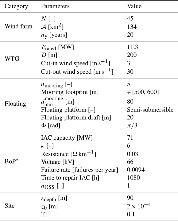
* BoP: balance of plant.
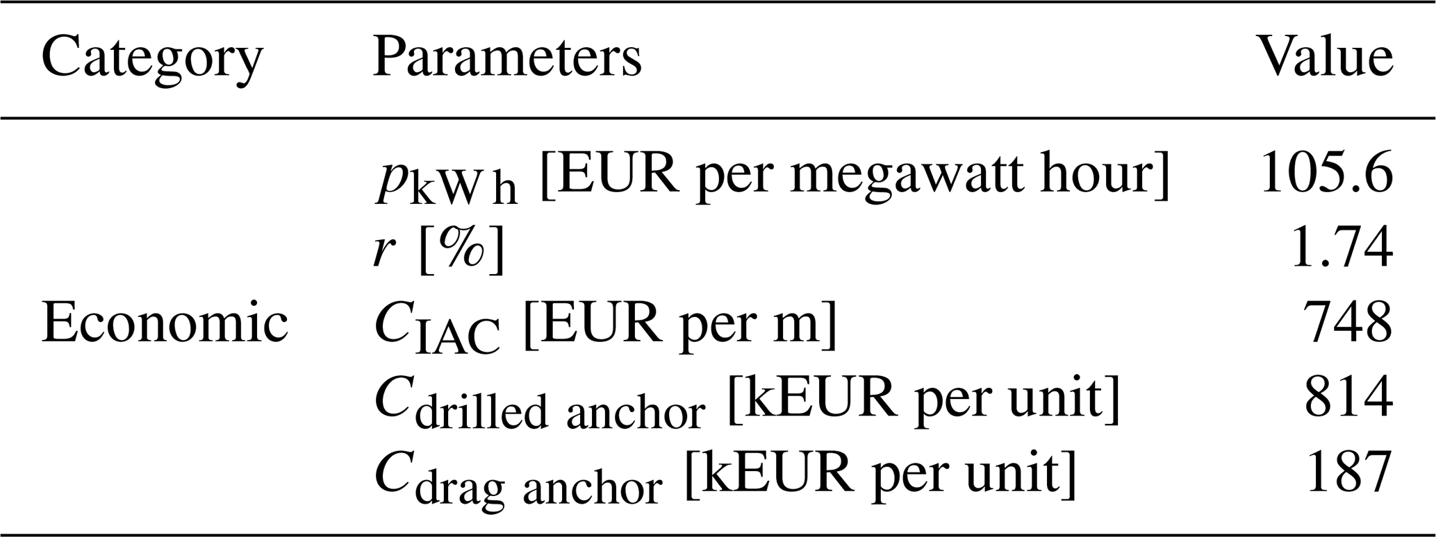
A2 Economic inputs
B1 Price of electricity
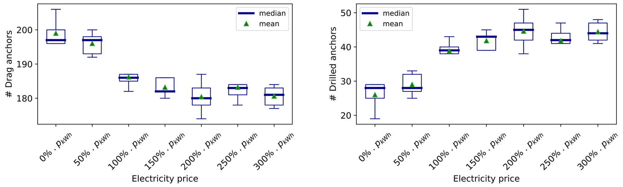
Figure B1Results of the sensitivity analysis on the electricity price – number of drag and drilled anchors.
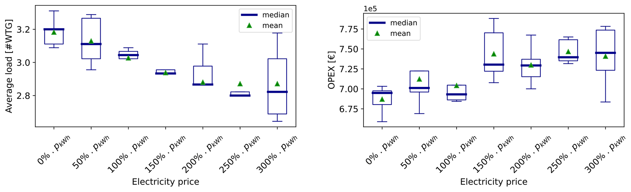
Figure B2Results of the sensitivity analysis on the electricity price – average load and OPEX.
B2 Anchors' cost
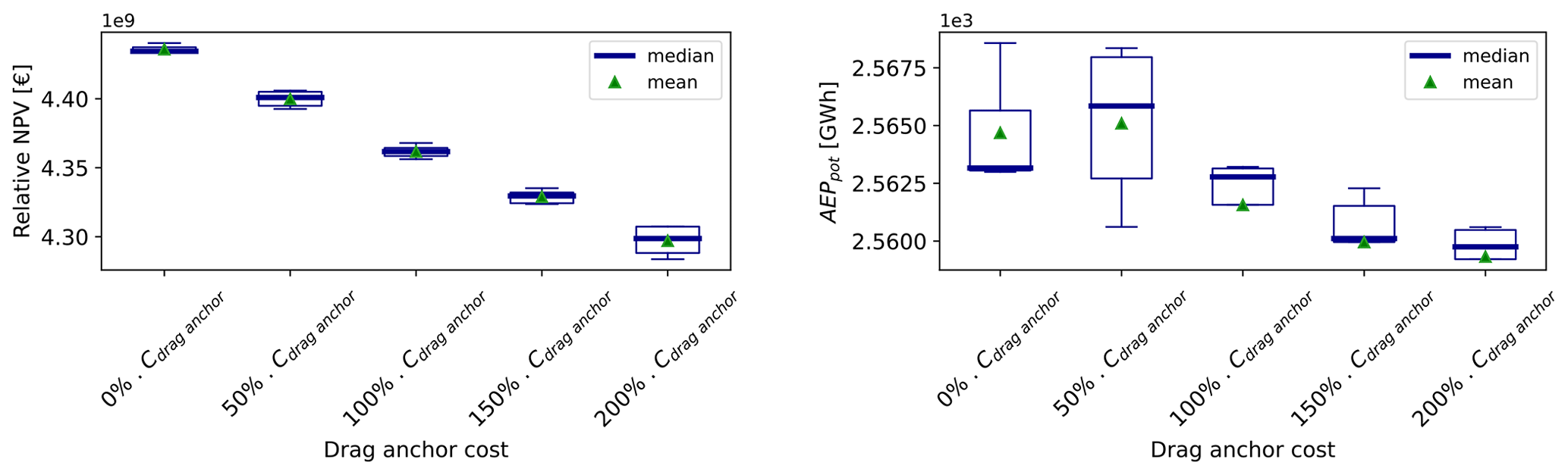
Figure B3Results of the sensitivity analysis on the anchor cost – relative NPV and potential AEP.
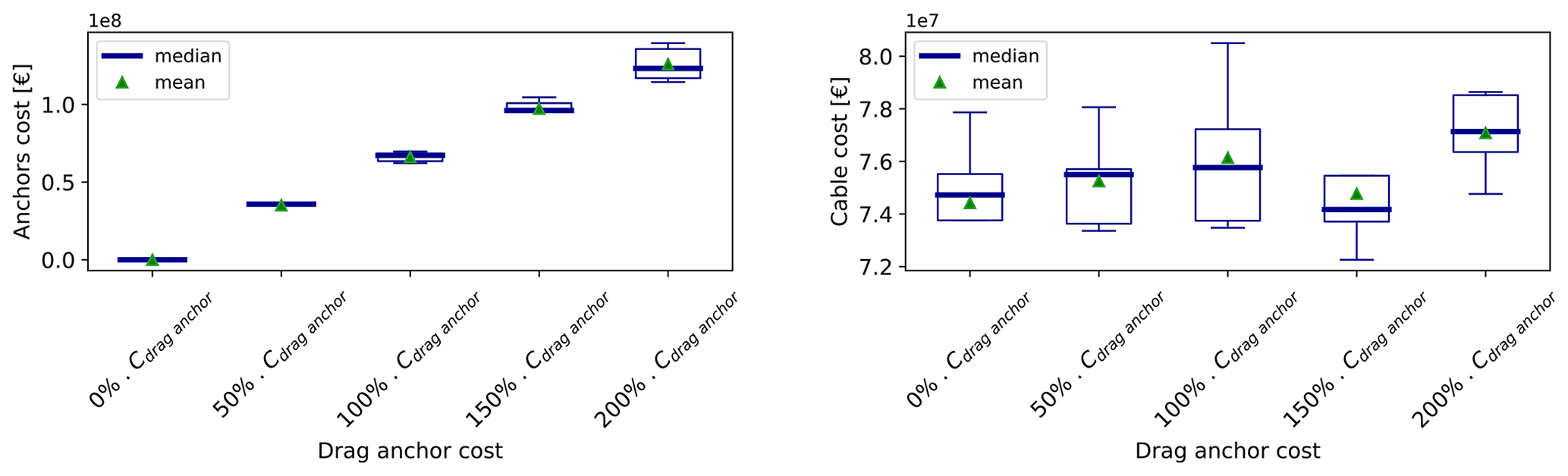
Figure B4Results of the sensitivity analysis on the anchor cost – anchor costs and cable cost.
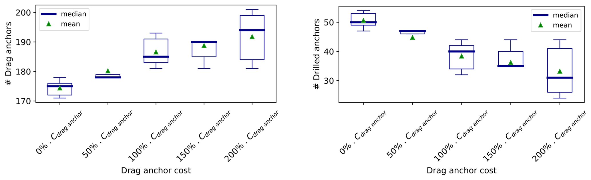
Figure B5Results of the sensitivity analysis on the anchor cost – number of drag and drilled anchors.
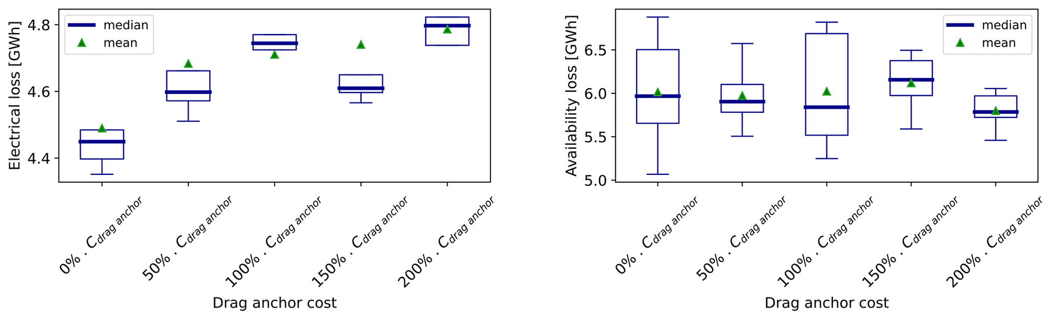
Figure B6Results of the sensitivity analysis on the anchor cost – electrical and availability losses.
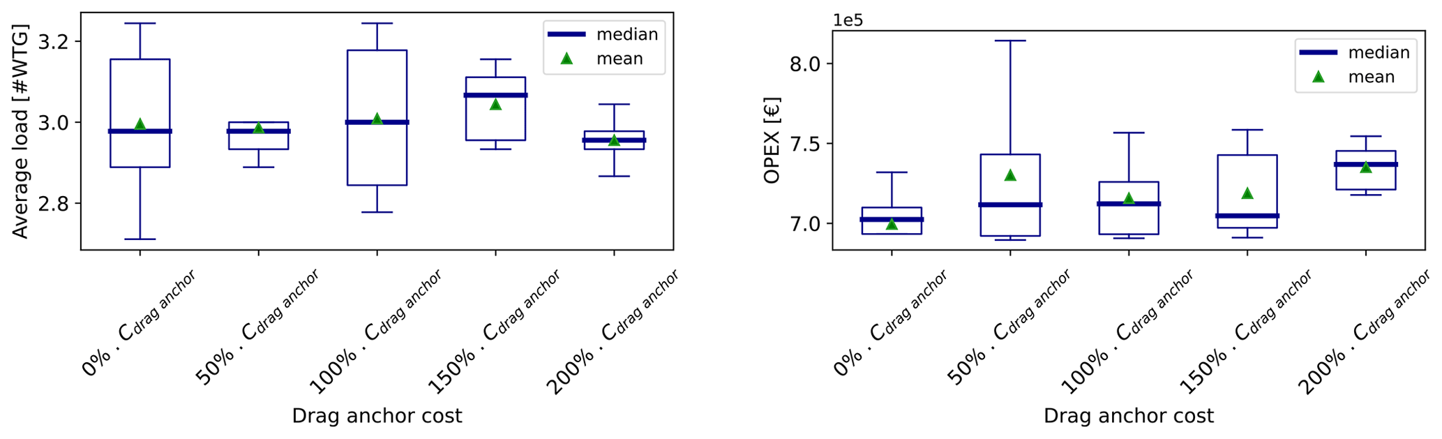
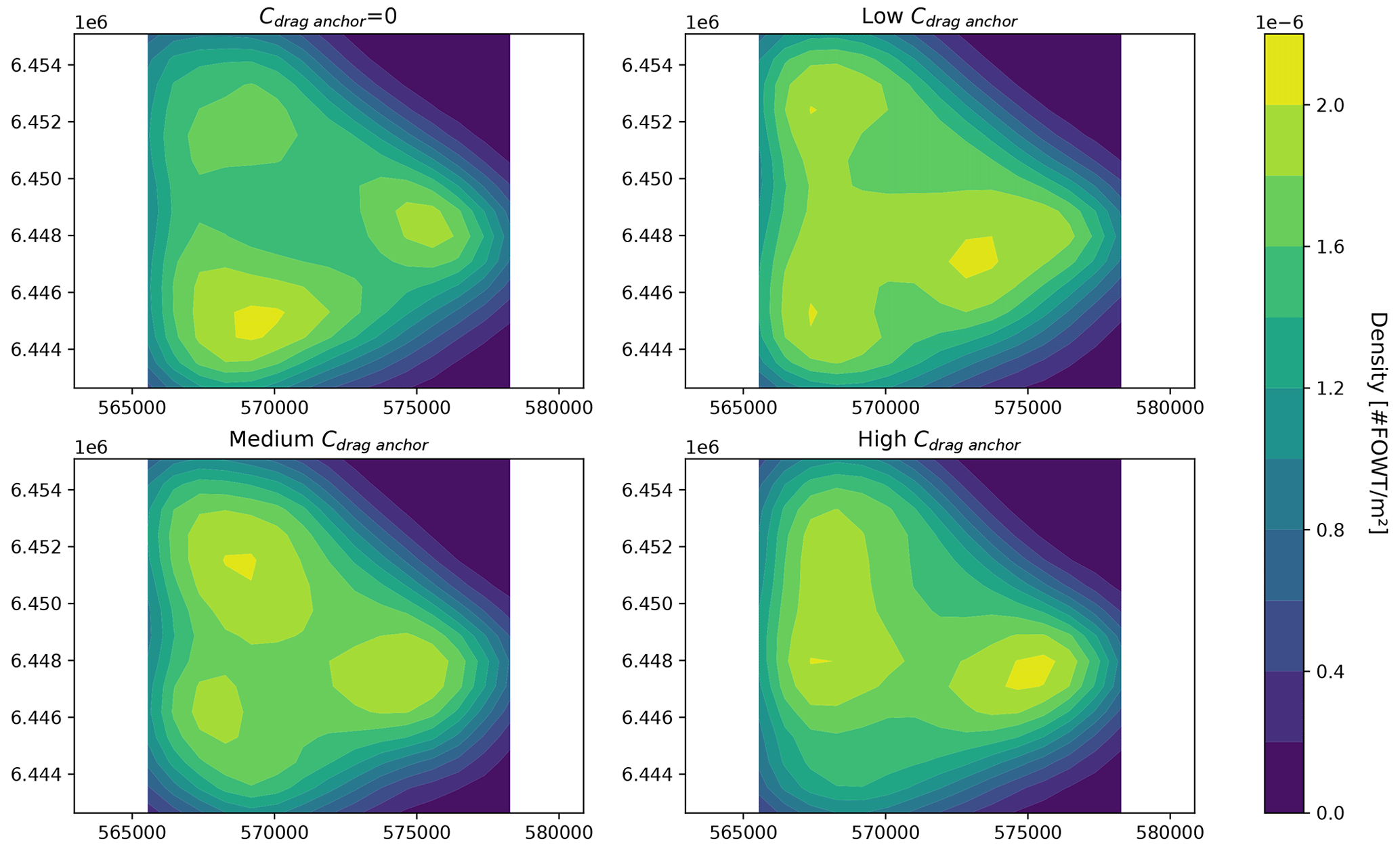
Figure B8Density heat maps of FOWT positions for different anchor cost levels; x axis: absolute easting [m]; y axis: absolute northing [m].
B3 Cable cost per unit length
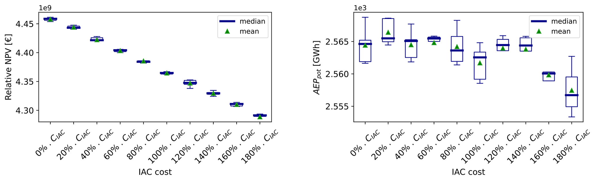
Figure B9Results of the sensitivity analysis on the cable cost per unit length – relative NPV and potential AEP.
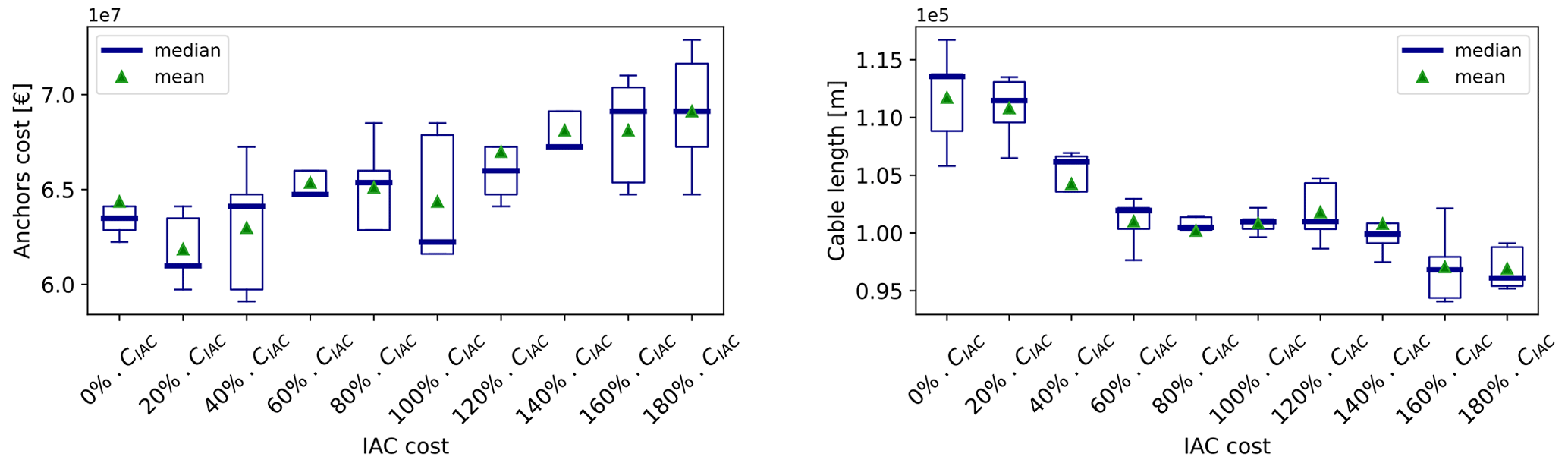
Figure B10Results of the sensitivity analysis on the cable cost per unit length – anchor costs and cable length.
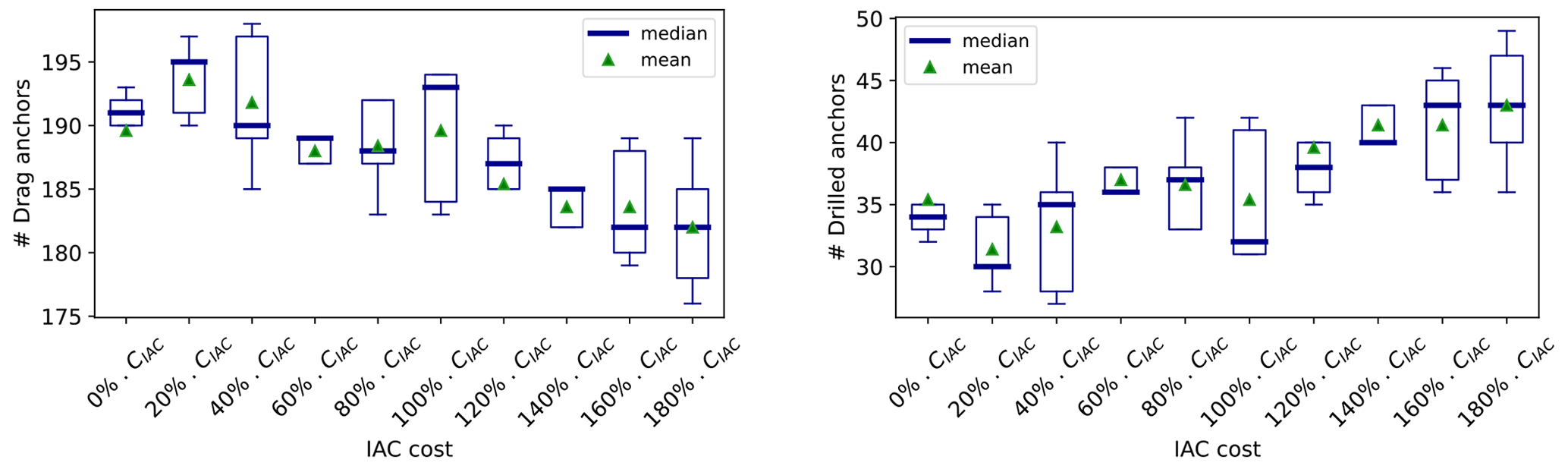
Figure B11Results of the sensitivity analysis on the cable cost per unit length – number of drag and drilled anchors.
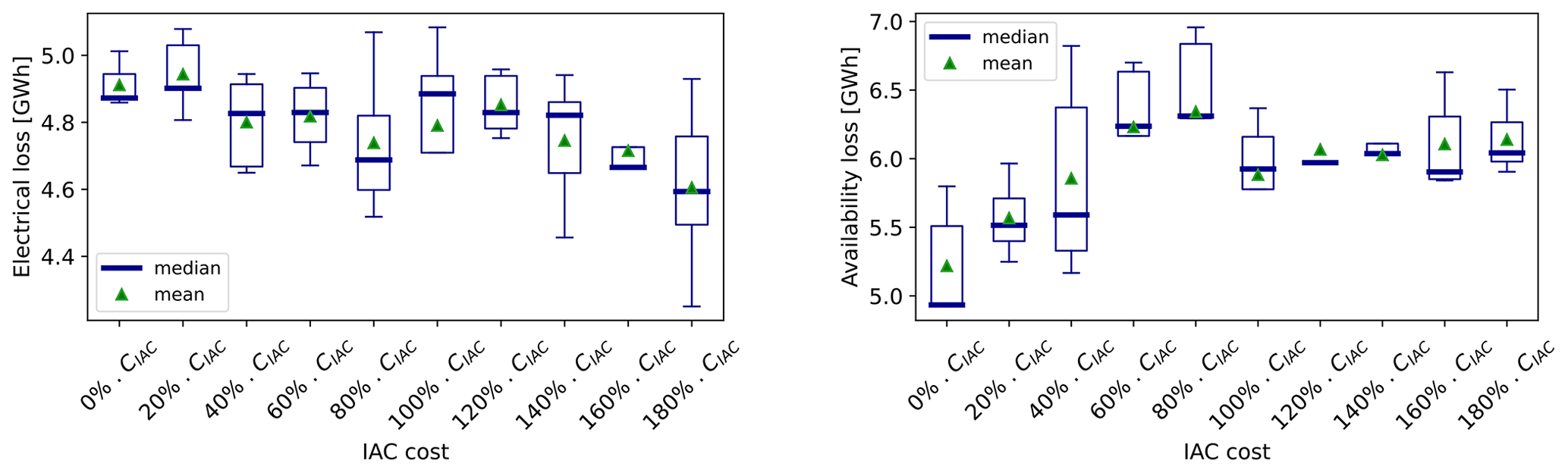
Figure B12Results of the sensitivity analysis on the cable cost per unit length – electrical and availability losses.
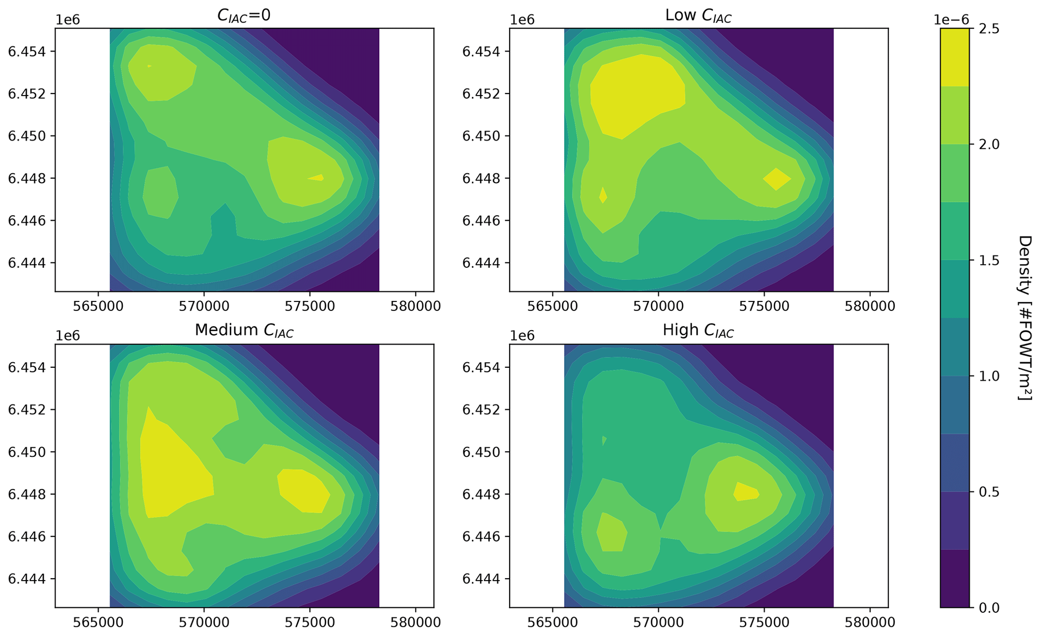
Figure B14Density heat maps of FOWT positions for different cable cost per unit length levels; x axis: absolute easting [m]; y axis: absolute northing [m].
The code is not publicly accessible as it was developed for PEAK Wind – Renewable Services and is used for commercial purposes by the latter. The Python library TopFarm (https://topfarm.pages.windenergy.dtu.dk/TopFarm2/index.html, Riva et al., 2024) by DTU and the module “interarray” by Souza de Alencar (2022) were used in the code.
The seabed data are from the General Bathymetric Chart of the Oceans (GEBCO) and are publicly available (https://download.gebco.net/, GEBCO, 2024).
IB, THS and KD proposed, supported and reviewed the present work. AIHi proposed the assumptions and methodology, programmed the models, created the simulations, and wrote the results and conclusions. AIH also edited the present paper.
At least one of the (co-)authors is a member of the editorial board of Wind Energy Science. The peer-review process was guided by an independent editor, and the authors also have no other competing interests to declare.
Publisher's note: Copernicus Publications remains neutral with regard to jurisdictional claims made in the text, published maps, institutional affiliations, or any other geographical representation in this paper. While Copernicus Publications makes every effort to include appropriate place names, the final responsibility lies with the authors.
Amalia Ida Hietanen would like to thank her supervisors for their guidance, expertise and support throughout the project. In addition, she would like to acknowledge PEAK Wind for accommodating the creation of a scientific hub for development to benefit the wind industry.
This paper was edited by Erin Bachynski-Polić and reviewed by Markus Jürgen Lerch and one anonymous referee.
Charhouni, N., Sallaou, M., and Mansouri, K.: Realistic wind farm design layout optimization with different wind turbines types, Int. J. Energ. Environ. Eng., 10, 307–318, https://doi.org/10.1007/s40095-019-0303-2, 2019. a, b
DTOcean: Deliverable 4.6: Framework for the prediction of the reliability, economic and environmental criteria and assessment methodologies for Moorings and Foundations, in: DTOcean – Optimal Design Tools for Ocean Energy Arrays, https://www.researchgate.net/publication/308265985_Framework_for_the_prediction_of_the_reliability_economic_and_environmental_criteria_and_assessment_methodologies_for_Moorings_and_Foundations_Deliverable_46_of_the_DTOcean_project (last access: 19 February 2024), 2015. a
EMD: windPRO 3.6 User Manual: OPTIMIZE, EMD International A/S, https://help.emd.dk/knowledgebase/content/windPRO3.6/c8-UK_WindPRO3.6-OPTIMIZATION.pdf (last access: 19 February 2024), 2022. a
Feng, J. and Shen, W. Z.: Solving the wind farm layout optimization problem using random search algorithm, Renew. Energy, 78, 182–192, https://doi.org/10.1016/j.renene.2015.01.005, 2015. a
Froese, G., Ku, S. Y., Kheirabadi, A. C., and Nagamune, R.: Optimal layout design of floating offshore wind farms, Renew. Energy, 190, 94–102, https://doi.org/10.1016/j.renene.2022.03.104, 2022. a, b
GEBCO: GEBCO Gridded Bathymetry Data Download, https://download.gebco.net/ (last access: 19 February 2024), 2024. a
Lackner, M. A. and Elkinton, C. N.: An Analytical Framework for Offshore Wind Farm Layout Optimization, Wind Eng., 31, 17–31, 2007. a
Lerch, M., De-Prada-Gil, M., and Molins, C.: A metaheuristic optimization model for the inter-array layout planning of floating offshore wind farms, Int. J. Elect. Power Energ. Syst., 131, 107128, https://doi.org/10.1016/j.ijepes.2021.107128, 2021. a, b
Lieng, J. T., Sturm, H., and Hasselø, K. K.: Dynamically installed anchors for floating offshore wind turbines, Ocean Eng., 266, 112789, https://doi.org/10.1016/j.oceaneng.2022.112789, 2022. a
Mahfouz, M. Y., Hall, M., and Cheng, P. W.: A parametric study of the mooring system design parameters to reduce wake losses in a floating wind farm, J. Phys.: Conf. Ser., 2265, 042004, https://doi.org/10.1088/1742-6596/2265/4/042004, 2022. a
Maienza, C., Avossa, A., Ricciardelli, F., Coiro, D., Troise, G., and Georgakis, C.: A life cycle cost model for floating offshore wind farms, Appl. Energy, 266, 114716, https://doi.org/10.1016/j.apenergy.2020.114716, 2020. a
Marcus, M. M.: Briefing: ScotWind Leasing for offshore wind, https://www.crownestatescotland.com/sites/default/files/2023-08/scotwind-briefing-november-2022.pdf (last access: 19 February 2024), 2022. a
Mosetti, G., Poloni, C., and Diviacco, B.: Optimization of wind turbine positioning in large windfarms by means of a genetic algorithm, J. Wind Eng. Indust. Aerodynam., 51, 105–116, https://doi.org/10.1016/0167-6105(94)90080-9, 1994. a
Pedersen, M. M., Forsting, A. M., van der Laan, P., Riva, R., Romàn, L. A. A., Risco, J. C., Friis-Møller, M., Quick, J., Christiansen, J. P. S., Rodrigues, R. V., Olsen, B. T., and Réthoré, P.-E.: PyWake 2.5.0: An open-source wind farm simulation tool, https://gitlab.windenergy.dtu.dk/TOPFARM/PyWake (last access: 19 February 2024), 2023. a
Pillai, A. C., Chick, J., Khorasanchi, M., Barbouchi, S., and Johanning, L.: Application of an offshore wind farm layout optimization methodology at Middelgrunden wind farm, Ocean Eng., 139, 287–297, https://doi.org/10.1016/j.oceaneng.2017.04.049, 2017. a
Ramírez, L., Fraile, D., and Brindley, G.: Offshore Wind in Europe, Tech. rep., Wind Europe, https://windeurope.org/intelligence-platform/product/offshore-wind-in-europe-key-trends-and-statistics-2020/ (last access: 19 February 2024), 2020. a
Rentschler, M. U.: Design optimization of dynamic inter-array cable systems for floating offshore wind turbines, Renew. Sustain. Energ. Rev., 111, 622–635, https://doi.org/10.1016/j.rser.2019.05.024, 2019. a, b
Rentschler, M. U. T.: Parametric study of dynamic inter-array cable systems for floating offshore wind turbines, Mar. Syst. Ocean Technol., 15, 16–25, https://doi.org/10.1007/s40868-020-00071-7, 2020. a
Riva, R., Liew, J. Y., Friis-Møller, M., Krasimirov Dimitrov, N., Barlas, E., Réthoré, P.-E., and Pedersen, M. M.: Welcome to TOPFARM, https://topfarm.pages.windenergy.dtu.dk/TopFarm2/index.html (last access: 19 February 2024), 2024. a
Rodrigues, S., Bauer, P., and Bosman, P. A.: Multi-objective optimization of wind farm layouts – Complexity, constraint handling and scalability, Renew. Sustain. Energ. Rev., 65, 587–609, 2016. a, b
Ros, M. and James, R.: Floating Offshore Wind – Market & Technology Review, Tech. rep., Carbon Trust, https://www.carbontrust.com/our-work-and-impact/guides-reports-and-tools/floating-offshore-wind-market-technology-review (last access: 19 February 2024), 2015. a
Souza de Alencar, M.: Optimization heuristics for offshore wind power plant collection systems design, Optimeringsheuristik til design af opsamlingssystemer til offshore vindkraft, MS thesis, DTU Department of Wind and Energy Systems, https://github.com/mdealencar/interarray/blob/main/README.md (last access: 19 February 2024), 2022. a, b
Tesauro, A., Réthoré, P.-E., and Larsen, G. C.: State of the art of wind farm optimization, Proceedings of Ewea 2012 – European Wind Energy Conference; Exhibition, 3, 16–19 April 2012, Copenhagen, Denmark, 2020–2030, http://events.ewea.org/annual2012/ (last access: 19 February 2024), 2012. a, b
Zhang, Q., Wang, X., Du, W., Zhang, H., and Li, X.: Reliability Model of Submarine Cable Based on Time-varying Failure Rate, IEEE Xplore, 10, 711–715, https://doi.org/10.1109/APAP47170.2019.9224914, 2019. a