the Creative Commons Attribution 4.0 License.
the Creative Commons Attribution 4.0 License.
 | 04 Apr 2024
HyDesign: a tool for sizing optimization of grid-connected hybrid power plants including wind, solar photovoltaic, and lithium-ion batteries
Hajar Habbou
Mikkel Friis-Møller
Megha Gupta
Rujie Zhu
Kaushik Das
Hybrid renewable power plants consisting of collocated wind, solar photovoltaic (PV), and lithium-ion battery storage connected behind a single grid connection can provide additional value to the owners and society in comparison to individual technology plants, such as those that are only wind or only PV. The hybrid power plants considered in this article are connected to the grid and share electrical infrastructure costs across different generation and storing technologies. In this article, we propose a methodology for sizing hybrid power plants as a nested-optimization problem: with an outer sizing optimization and an internal operation optimization. The outer sizing optimization maximizes the net present values over capital expenditures and compares it with standard designs that minimize the levelized cost of energy. The sizing problem formulation includes turbine selection (in terms of rated power, specific power, and hub height), a wind plant wake loss surrogate, simplified wind and PV degradation models, battery degradation, and operation optimization of an internal energy management system. The problem of outer sizing optimization is solved using a new parallel “efficient global optimization” algorithm. This new algorithm is a surrogate-based optimization method that ensures a minimal number of model evaluations but ensures a global scope in the optimization. The methodology presented in this article is available in an open-source tool called HyDesign. The hybrid sizing algorithm is applied for a peak power plant use case at different locations in India where renewable energy auctions impose a monetary penalty when energy is not supplied at peak hours. We compare the hybrid power plant sizing results when using two different objective functions: the levelized cost of energy (LCoE) or the relative net present value with respect to the total capital expenditure costs (). Battery storage is installed only on -based designs, while the hybrid design, including wind, solar, and battery, only occurs on the site with good wind resources. Wind turbine selection on this site prioritizes cheaper turbines with a lower hub height and lower rated power. The number of batteries replaced changes at the different sites, ranging between two or three units over the lifetime. A significant oversizing of the generation in comparison to the grid connection occurs on all -based designs. As expected LCoE-based designs are a single technology with no batteries.
- Article
(4575 KB) - Full-text XML
- BibTeX
- EndNote


A hybrid power plant (HPP) consisting of collocated wind, photovoltaic (PV), and lithium-ion battery storage connected behind a single grid connection point can provide better returns on investment than individual-source (wind or solar) plants in locations where the wind and solar resources are comparable and for electricity markets in which fixed power purchase agreement electricity prices are not possible. HPPs can be designed to have operational flexibility in terms of dispatchability and ancillary service provision that makes them closer to traditional power plants in terms of achieving additional profitability in markets with time-varying electricity prices under grid connection constraints and that have reduced costs due to the shared infrastructure (Gorman et al., 2020; Dykes et al., 2020).
Sizing of HPPs is a multi-disciplinary design analysis and optimization (MDAO) problem that requires detailed modeling of the wind and solar resources as well as the wind, PV, and storage performance, costs, and operation (Dykes et al., 2020). Additionally, the selection of the wind turbine (WT) characteristics (specific power, hub height) and PV characteristics (panel orientation) are additional degrees of freedom that can significantly modify the results of the sizing. Traditional objective functions of the sizing optimization problem are maximizing net annual energy production or minimizing LCoE (Tripp et al., 2022), but, in general, HPP designs that include energy storage can produce more revenue relative to the cost increase. In this article, we compare HPP sizing optimization for both LCoE and relative net revenue as objective functions.
A detailed energy management system (EMS) is required to determine the operation of the battery, given the time series of wind and solar generation and the battery's capacity. EMS optimization will determine when to charge and discharge the battery with the objective of maximizing the revenue obtained by the HPP. Several articles focus on formulating EMS optimization problems and propose different formulations (Al-Lawati et al., 2021; Das et al., 2020; Khaloie et al., 2021a, b; Wang et al., 2019). Different levels of complexity can be studied in the implementation of EMS, such as (1) rule-based algorithms that prescribe the operation of the battery, (2) deterministic EMS optimization that maximizes the revenue assuming perfect forecasts (full future knowledge) of the price of electricity and the wind and solar generation time series, (3) robust optimization of EMS operation providing battery operation under worst-case scenarios of forecast errors in generation and price time series, and (4) stochastic optimization of EMS operation that provides the best operation over the entire distribution of forecasting error. EMS operational optimization within the HPP sizing optimization is not common in the literature, but it is required to unravel the value of HPP fully.
Furthermore, HPP sizing requires solving the long-term performance of the different components through the lifetime of the HPP; this implies modeling the degradation in the performance of the individual components. Li-ion (lithium-ion) batteries, wind turbines, and PV cells have significant degradation over time. Several models of PV degradation exist (Jordan et al., 2016), and PV manufacturers can provide a warranty in line with the degradation curve, while recent publications report measured PV degradation rates (Theristis et al., 2023, 2020). Wind turbine degradation significantly more complex than performance degradation, e.g., due to blade erosion (López et al., 2023; Panthi and Iungo, 2023; Bech et al., 2018), is compensated by the internal wind turbine pitch control system. Several studies report different levels of wind plant degradation as losses of capacity factor over age (Hamilton et al., 2020; Jia et al., 2016; Staffell and Green, 2014; Astolfi et al., 2022).
Typically, battery cells have to be replaced when their capacity degrades beyond a manufacturer-defined safety threshold. The higher costs due to battery replacement play a dominant role in total battery costs. Therefore, considering battery degradation when sizing HPPs can optimize the use of batteries, extending battery lifetime and reducing costs. Battery degradation is a complicated chemical process. Theoretical studies (Safari et al., 2008; Vetter et al., 2005) on battery degradation explain the detailed degradation mechanism of battery cells. However, the required parameters and conditions of the battery cell can not be obtained in the sizing stage. To incorporate the battery degradation model into the sizing problem, it is possible to use semi-empirical models (Xu et al., 2016) that only require the state of charge (SoC) time series as input to assess battery lifetime. This model considers the solid electrolyte interphase film formation theory calibrated based on experimental observations, and it can describe the non-linear degradation process.
To the authors' knowledge, there is no available sizing methodology for the design of utility-scale grid-constrained hybrid power plants considering all the above-mentioned characteristics. This article presents a general methodology for hybrid plant sizing as a nested optimization, including several novel aspects: (1) turbine selection, (2) PV and wind degradation, (3) internal EMS operation optimization, and (4) battery degradation based on resulting load cycles. We apply the methodology and report the detailed result of the hybrid plant design in three different locations in India for sites with the following characteristics: (a) good solar, (b) good wind, and (c) bad solar and bad wind. The research objective is to build a framework for optimization of hybrid power plants that is flexible, is modular, and can be extended to solve the sizing and physical design of HPPs.
India is a large market in which HPPs could become important because of the need to provide renewable energy that supports the demand patterns and because of the intermediate solar and wind resources. For this reason, Indian sites are used as example cases in this article.
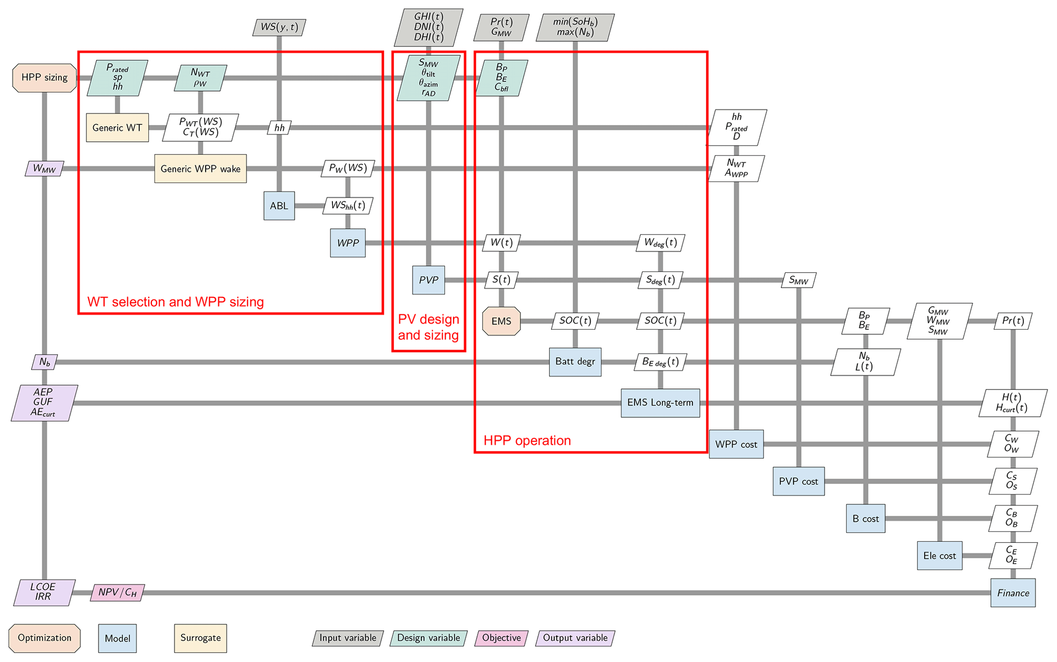
The design of an HPP is an optimization problem that involves several sub-optimization problems such as WT selection, wind power plant (WPP) siting and layout optimization, PV array sitting, EMS operation optimization coupled with battery degradation, and electrical infrastructure optimization. HPP sizing optimization focused on maximizing the viability of an HPP installation in a given location requires a simplified approach. The XDSM (eXtended Design Structure Matrix) diagram of the proposed nested optimization for HPP sizing is presented in Fig. 1. In this sizing optimization formulation several simplifications have been performed to reduce the complexity of the optimization. (1) The WT layout optimization is replaced by a surrogate of the wakes of sub-optimal WPPs. (2) Uncoupled battery, wind, and PV degradation models are used to reduce the complexity of the EMS optimization: the internal operation optimization solves a short-term EMS problem without considering battery degradation but with a penalty for battery power ramping, while a long-term operation rule-based EMS (EMS long-term) corrects the ideal battery operation for degradation and forecast errors. (3) Simplified electrical infrastructure costs are used, instead of an electrical cable and infrastructure optimization. (4) No interaction between WT and PV is assumed, neglecting PV losses due to shadows and flickering and changes in the wind boundary layer due to the presence of large PV arrays.
2.1 HPP sizing optimization
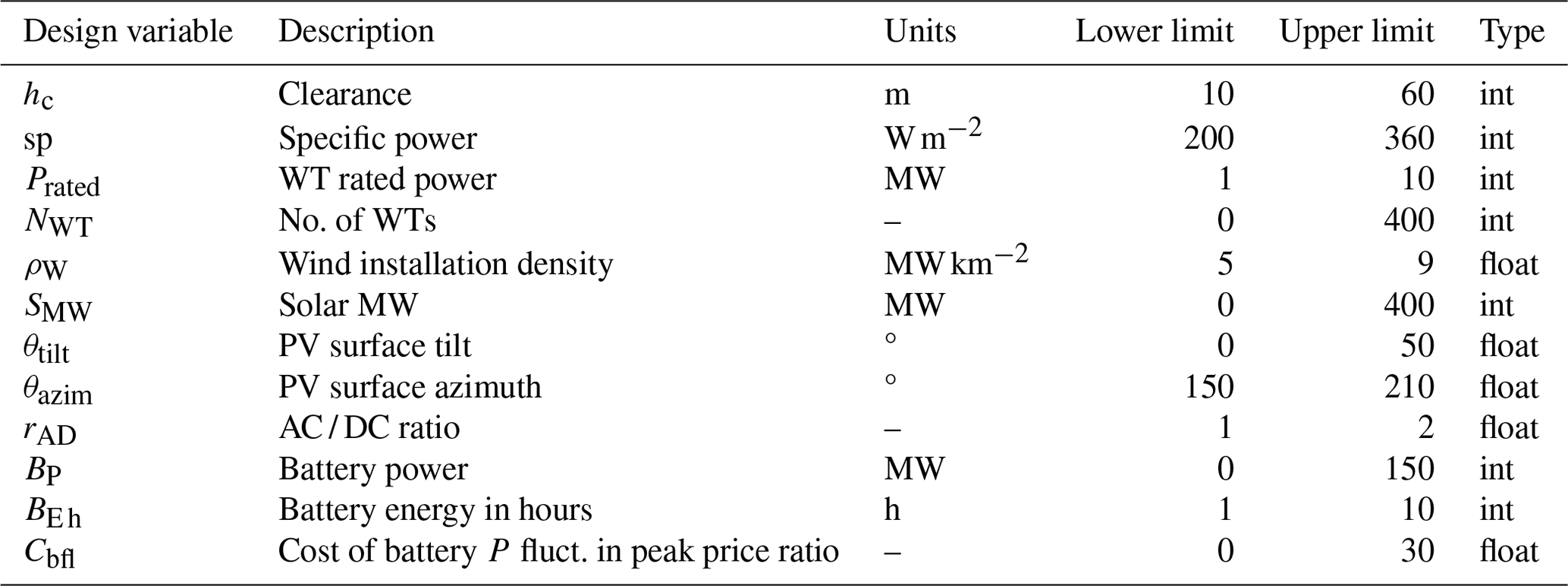
The HPP sizing optimization problem consists of minimizing LCoE or maximizing (relative net present value with respect to the total capital expenditure costs) by changing the design variables: height clearance of the rotor tip to the ground (hc in m), turbine's specific power (sp in MW m−2), turbine's rated power (Prated in MW), number of wind turbines (NWT), wind installation density (ρW in MW km−2), solar capacity (SMW in MW), PV tilt angle (θtilt in degrees), PV azimuth angle (θazim in degrees), PV inverter AC / DC ratio (rAD), battery power capacity (BP in MW), battery energy storage capacity in hours at battery power capacity (BE h), and battery fluctuation penalty factor (Cbfl). Furthermore, the sizing can be forced to only take integer values on some specific design variables such as NWT.
2.2 Generic wind turbine
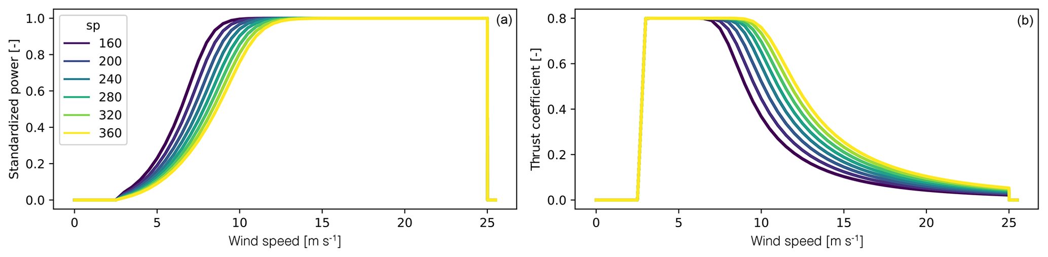
A lookup table is built based on DTU's (Technical University of Denmark) PyWake generic turbine model (Pedersen et al., 2023). The interpolation of this data is a surrogate that predicts the power and thrust coefficient curves, given the turbine's specific power, defined as the ratio between the rated power and the rotor area (). The wind turbine power curve and thrust coefficient curves as a function of the wind speed (WS) are represented as PWT(WS) and CT(WS) in Fig. 1. Examples of the surrogate power and thrust coefficient curves are given in Fig. 2. The rotor diameter () and hub height () can be computed based on sp and the clearance height.
2.3 Generic wind power plant wake model
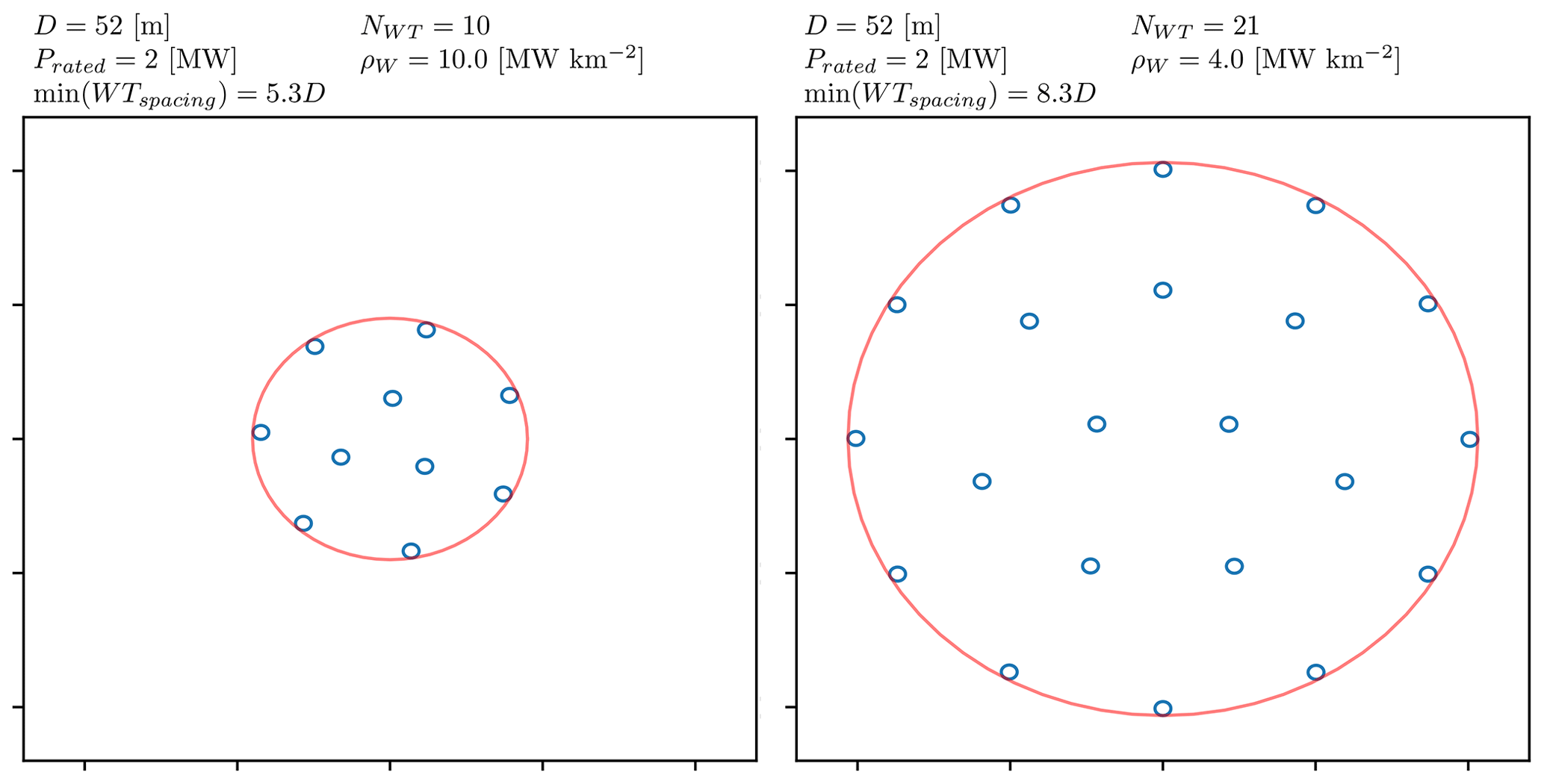
A database of wind power plants is generated using circular plant borders and a simplified layout optimization that maximizes the distance between the turbines. Two example layouts are presented in Fig. 3. Here it can be seen that the layouts are symmetric, and the minimum WT spacing is the consequence of specifying the number of turbines (NWT), the turbine rated power (Prated), and the installation density (ρW, plant-rated power over the land use area, MW km−2). Wakes are simulated using PyWake's implementation of Zong's wake model (Pedersen et al., 2023; Zong and Porté-Agel, 2020) which combines a Gaussian wind speed deficit with local turbulence-dependent linear wake expansion, with a squared sum wake deficit superposition model and Frandsen's added turbulence model as specified in the International Electrotechnical Commission (IEC) wind turbine design standard (IEC, 2017).
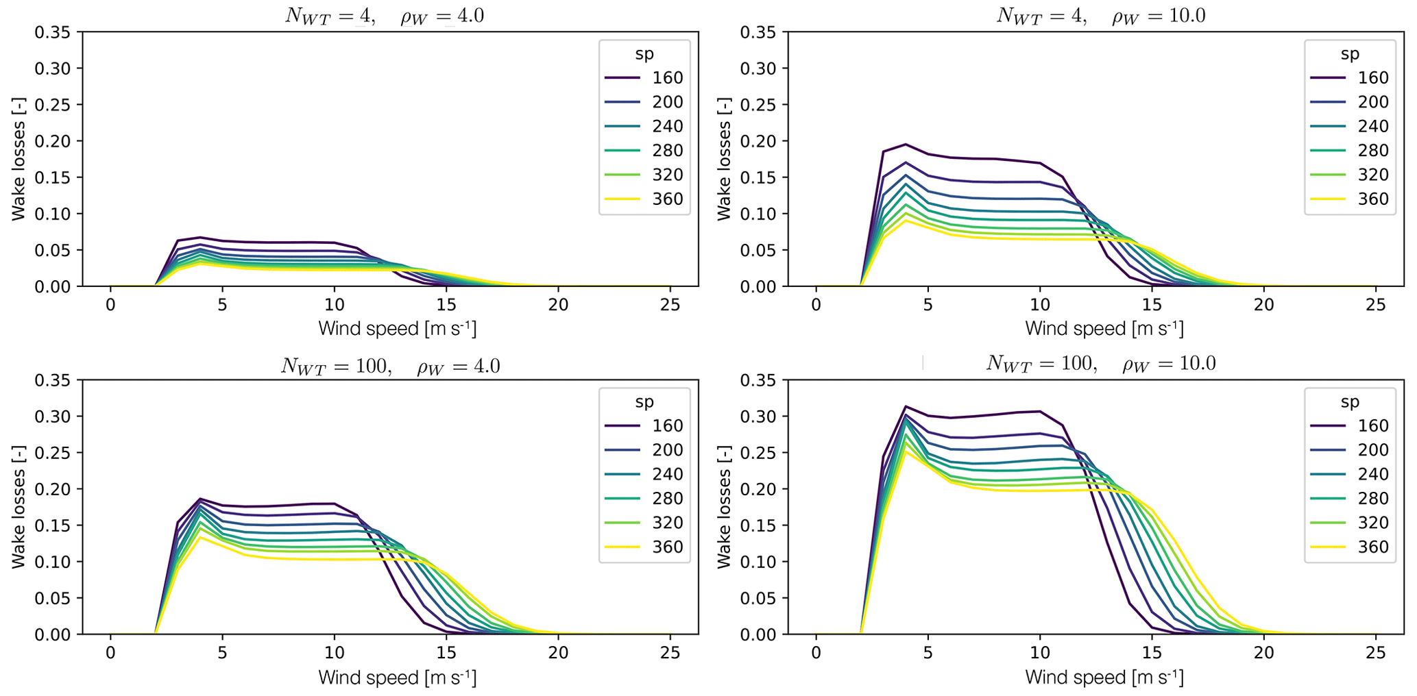
Figure 4Example wake losses as a function of the number of turbines, installation density, and WT's specific power.
Detailed wake losses as a function of wind speed and wind direction are simulated for multiple WPP layouts with the same number of turbines (NWT) and installation density (ρW) for a given WT's specific power, hence given power and thrust curves. The resulting wake losses are aggregated, taking the larger 90th quantile across wind directions and across 20 layouts generated using a different random seed number. A surrogate of the wake losses curve as a function of the hub height wind speed (WL(WS)) is built as a function of the installation density, number of turbines, and specific power of the turbine. Example results of the surrogate are presented in Fig. 4. Finally, the generic wind plant model will combine the turbine power curve with the expected wake losses to provide a wake-affected plant power curve (see Eq. 2).
2.4 Weather
ERA5 (Hersbach et al., 2020) is used as a reanalysis dataset for wind resource calculations. The hourly wind velocity time series with a 0.25° × 0.25° resolution in latitude and longitude are interpolated into heights of 50, 100, 150, and 200 m. This dataset is stored and interpolated at the location of hybrid power plants using linear interpolation in the horizontal coordinates, keeping the hub height dimension of the velocities to compute the effect of changing the hub height of the turbines in the optimization.
The mean wind speed from the Global Wind Atlas 2 (GWA2) is used for correcting ERA5's mean wind speed following the approach presented in (Murcia et al., 2022). This scaling correction is necessary to include the first-order effects of terrain. The corrected wind speed time series is provided at multiple heights (WS(y,t)) in the atmospheric boundary layer (ABL) model. This model uses a piecewise power law interpolation to determine the wind speed time series at the hub height (WShh(t)).
ERA5-Land is used as a reanalysis of the hourly global horizontal irradiance time series (GHI(t)) because it has a higher horizontal resolution than ERA5 (0.1° × 0.1°), and it shows better validation metrics for individual PV plant generation modeling (Camargo and Schmidt, 2020). Decomposition of GHI into direct normal irradiance (DNI) and diffuse horizontal irradiance (DHI) is done in two steps: the Direct Insolation Simulation Code (DISC) model is used to estimate the DNI (Maxwell, 1987) using the GHI and relative air mass model (Kasten and Young, 1989), while the DHI is estimated using the solar position (θzenith(t)) (see Eq. 3).
2.5 Wind power plant (WPP) model
The wind generation time series (W(t)) is obtained by interpolating the plant power curve at the hub height's wind speed time series, scaling the generation by the installed capacity. Additionally, efficiency is assumed to cover the electrical and availability losses (see Eq. 4).
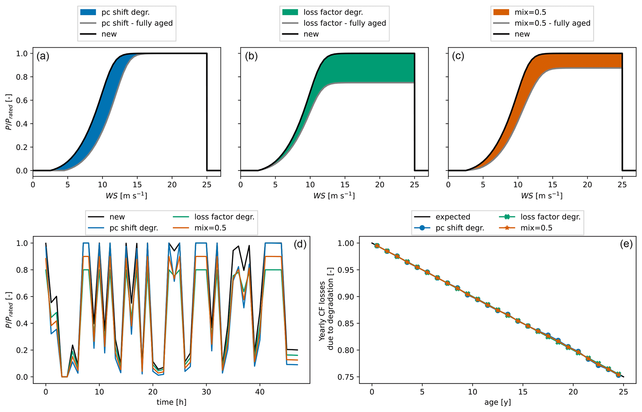
Figure 5(a–c) Mechanisms of WT degradation: (a) shift in the power curve (PC), (b) loss factor, and (c) 50 %–50 % mixture of both mechanisms. (d) Example of 2 d of WPP generation time series after 20 years. (e) Prescribed degradation curve and resulting losses in capacity factor (CF) over the WPP lifetime with the three mechanisms of WT degradation.
Wind turbine degradation is modeled as a mixture of two performance degradation mechanisms: (a) a shift in the power curve towards higher wind speeds represents blade degradation and increasing friction losses (López et al., 2023) and (b) a loss factor applied to the power time series represents an increase in availability losses. These mechanisms are depicted on the top plots in Fig. 5. The WT degradation curve (dlW(t)) prescribes the level of loss in capacity factor over time, and the power generation with degradation (Wdeg(t)) is obtained by linear interpolation of the generation time series of the new (Wnew) and fully degraded (Wfg) generations (see Eq. 5). A linear degradation on the wind turbine has been used in the study cases (see Fig. 5).
2.6 PV power (PVP) plant model
Power conversion uses pvlib (Holmgren et al., 2018) based on a 1 MW PV plant configuration using the default PV module (open rack with glass–glass PV construction) and inverter on pvlib with the irradiance projection transposition model (Davies et al., 1984), the Sandia PV Array Performance Model (SAPM) (Kratochvil et al., 2004), and the Sandia performance model for grid-connected PV inverters (Boyson et al., 2007). The final PV generation requires the PV plant capacity (SMW), the orientation of the panels in terms of tilt and azimuth angles (θtilt,θazim), the ratio between the DC and AC sides of the inverter (rDA), the irradiances (DNI, DHI), the wind speed close to ground (WS1(t)), and the ambient temperature (T1(t)) (see Eq. 6).
The PV degradation model has a loss factor that follows a prescribed PV degradation curve dlS(t). The solar generation time series with degradation is obtained by applying the loss factor to the generation (see Eq. 7). A linear degradation curve is used in the study cases.
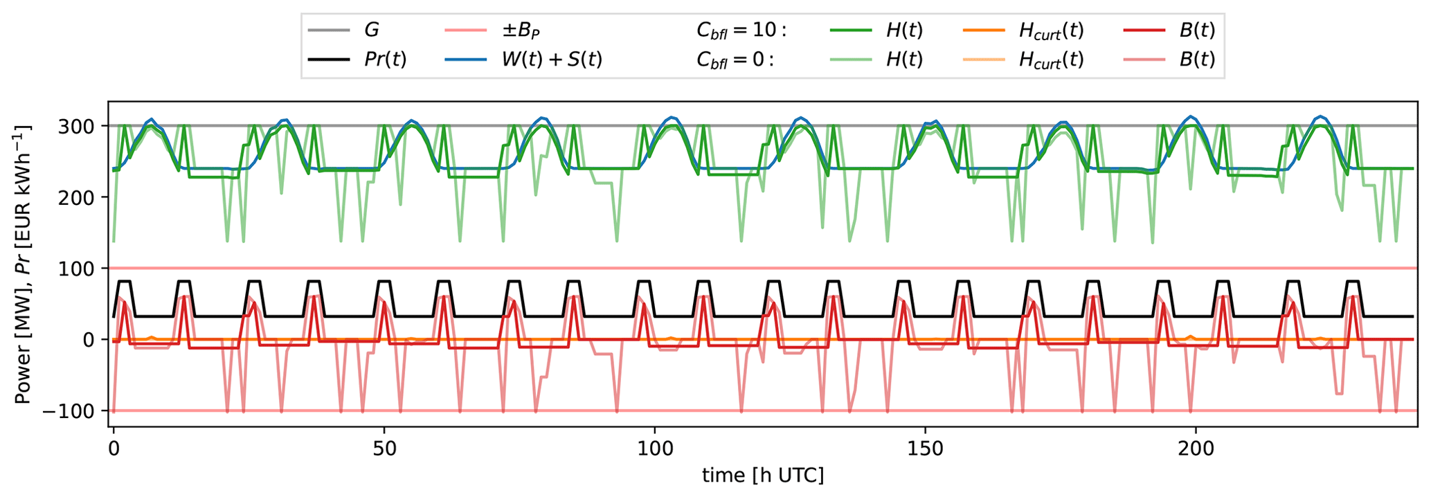
Figure 6EMS comparison in an example HPP for two different battery fluctuation penalty factors Cbfl.
2.7 Electricity price
The electricity price time series in the spot market (Pr(t)) is an input to the model; note that the price time series needs to be correlated with the weather time series. This article focuses on the valuation of time-varying power purchase agreements as the ones that have been seen in the Indian HPP market. This price signal has two levels of electricity price at peak and non-peak (high-demand) hours. An example of the peak–non-peak power purchase agreement (PPA) electricity price is presented in Fig. 6.
2.8 Energy management system (EMS) optimization model
The energy management system optimization model determines the optimal amount of battery charge or discharge and power curtailment that maximizes the revenue generated by the plant over a period of time, including a possible penalty for not meeting the requirement of energy generation and a penalty for battery power ramping to control the number of battery load cycles (see Eq. 8). The EMS optimization is solved using linear programming, applying a piecewise linearization to the change in battery efficiency in charge and discharge and to the absolute value of the battery power fluctuations. The EMS optimization does not account for battery, WT, or PV degradation and uses the generations without degradation. Furthermore, the EMS operation optimization assumes perfect knowledge of both the weather and price, and therefore, there are forecasting errors in neither the prices nor the weather.
The revenue is given by the product of electricity price (Pr(t)) and the HPP power generation (H(t)) minus the penalty over the period (l) and minus the battery ramping penalty (lb). The HPP generation is defined as the total power from wind (W(t)), PV (S(t)), battery charge or discharge (B(t)), and power curtailment (Pcurt(t)).
The penalty (l) is the missing energy generated at peak times with respect to the energy requirement over the period (El) times a mean peak electricity price (). The penalty can only be positive, which means that it can only subtract revenue and generation above the requirement does not yield additional revenue.
The battery fluctuation penalty (lb) is defined as the sum of the products of the absolute battery power fluctuations () and the difference between peak electricity price and the current price (Prpeak−Pr(t)). This means that large fluctuations in the battery charge or discharge are allowed when the price is high. The battery fluctuation penalty factor (Cbfl) is a design variable that captures how strongly the battery can be ramped, and therefore, it controls the battery degradation. When Cbfl is 0, then large changes in charge or discharge occur (see Fig. 6).
The constraints in the optimization force a minimum level of energy in the battery (ESoC(t)) when discharging (BE depth), ensure the limits due to batteries power capacity (BP) and energy capacity (BE=BE h BP), force the grid capacity (G), and include an asymmetric charging/discharging efficiency (ηcharge,ηdischarge).
2.9 Battery degradation model
The battery degradation model includes a linear degradation rate as a function of load cycles and a non-linear degradation due to the solid electrolyte interphase (SEI) film formation process in the early stage of the battery life. The rainflow-counting algorithm (Downing and Socie, 1982; Shi et al., 2018) is used to obtain the depth of discharge (RDoD,j), mean state of charge cycle (RSoC,j), and half or full cycle count (Rcount,j), for a number of load cycles (), given a relative state of charge time series (). The current age of the battery at each load cycle is defined as tc,j.
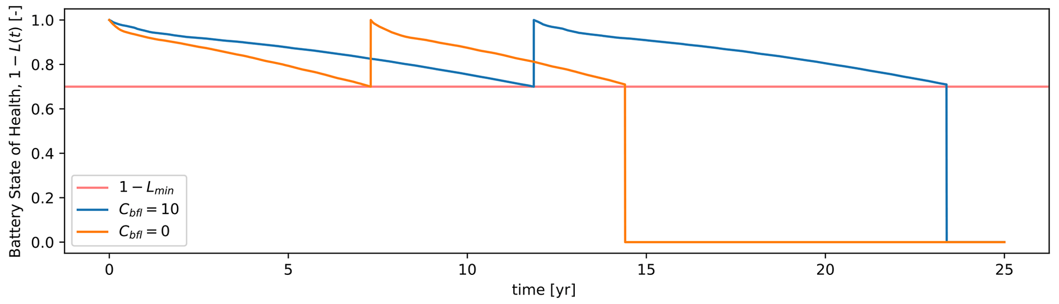
Figure 7Battery degradation comparison in an example HPP for two different battery fluctuation penalty factors Cbfl.
The linear degradation rate (fd) in Eq. (9) depends on a stress model due to the depth of discharge (SDoD), a stress model due to the age of the battery (St), a stress model due to the state of charge (SSoC), and a stress model due to cell temperature in kelvin (ST). The stress factor models are empirical relationships calibrated on measurements (Xu et al., 2016). Note that this model is considered linear because the degradation due to each cycle is summed over the lifetime. The parameters of the model are , , , kσ=1.04, σref=0.5, , Tref=293.15 (K), and .
The non-linear part of the degradation given in Eq. (10) describes the loss of storage capacity (LoC, L) using two models: a new battery and a used battery after the formation of SEI film. A predefined LoC level is used to determine the current regime of the battery (L1). L′ and are the LoC and linear estimation of LoC when L is equal to L1, where the parameters of the model are α=0.0575, β=121, and L1=0.92.
Finally, the time series of the degrading energy capacity of the battery is . In this article, the battery degradation model is not coupled to the EMS model, but instead, it uses the resulting state of charge time series (SoC(t)) estimated by the EMS optimization on an operation period (for example, 1 or 2 years). The SoC operation period is repeated to obtain the full lifetime of operation and then used to compute the degradation over the lifetime of the HPP. Finally, battery replacement occurs when the battery reaches a minimum health level (1−Lmin). Figure 7 presents a comparison of the degradation of the battery operating in the same HPP but using different battery fluctuation penalty factors.
2.10 Long-term operation (EMS long-term) correction model
A ruled-based EMS is implemented to account for battery, PV, and wind degradation and forecast errors in estimated wind and solar generation. The correction model consists of the following general principles: (1) try to follow the resulting operation obtained in the EMS described in Sect. 2.8 (B(t), ESoC(t)); (2) update the state of charge to account for the reduction in the available generation in the HPP and the new limits of the degraded battery; and (3) recompute the battery power operation and HPP curtailment, accounting for the charge and discharge efficiencies.
The implementation consists of computing the reduction in charging power due to the different available generations, as presented in Eq. (11). The SoC (ESoC LT(t)) is updated, including the constraints of the new energy limits of the degraded battery in Eq. (12). Finally, the battery's power (BLT(t)) to supply the SoC and the curtailment (Pcurt LT(t)) are updated in Eq. (13).
2.11 Wind plant costs model
A simple WPP cost model consists of estimating the total capital expenditure (CAPEX) costs (CW) and operational expenditure (OPEX) and maintenance costs (OW) as a function of the installed capacity (given as number of turbines times the rated power of the turbines: WMW=NWTPrated), the cost of the turbines, their construction, and civil infrastructure (CWT+CW civil). The OPEX is divided into fixed costs that are scaled with the rated capacity of the plant (OW fixed) and variable costs (OW var) that scale with the annual energy production of the wind turbines (AEPW) and the ratio between the reference turbine and selected turbine power rating. The wind turbine cost (Dykes et al., 2018) depends on the rotor diameter, the WT-rated power, and the tower hub height. This model uses empirical fits to estimate the mass of all WT components and, therefore, for simplicity, is not presented here. The final turbine costs are scaled with respect to the costs of a reference WT () (see Eq. 14).
2.12 PV plant costs model
A simple PV plant cost model consists of estimating the total capital expenditure (CAPEX) costs (CS) and operational expenditure (OPEX) and maintenance costs (OS) as a function of the installed capacity (SMW) and solar AC / DC ratio (rAD) (see Eq. 15). This model uses the PV costs per megawatt DC (CPV), the installation costs per megawatt DC (CS install), and fixed operational costs (OS fixed), while the inverter costs are provided per megawatt AC (Cinv).
2.13 Battery costs model
The battery plant cost model consists of estimating the total capital expenditure (CAPEX) costs (CB) and operational expenditure (OPEX) and maintenance costs (OB) as a function of the number of batteries required during the plant lifetime (Nb, assuming replacement of batteries after degradation), given the new battery energy (BE) and power capacities (BP) (see Eq. 16). The CAPEX model splits the energy capacity costs (CB E) and power-capacity-dependent costs, which include power capacity, installation, and control system costs (). An equivalent number of present batteries (NB eq) is used to reflect the decrease in battery cost throughout the lifetime of the battery, given a battery price reduction per year (fB) and the time of replacement of the battery (ib) in years (yb(ib)).
2.14 Electrical and shared infrastructure cost model
A simple electrical infrastructure cost model consists of estimating the total capital expenditure (CAPEX) costs (CE) as a function of the grid capacity (GMW) and the balance-of-system costs and grid connection costs (CBOS+Cgrid) and land costs (see Eq. 17). Note that the HPP land use area is shared between wind (AW) and solar (AS), given their corresponding installation densities: ρW and ρS.
2.15 HPP financial model
A simple financial model uses the weighted average cost of capital (WACC) for wind, PV, and battery as a discount rate (see Eq. 18). The WACC after tax (WACCtx) is the result of weighting the sum of the WACCs for wind, PV, battery, and electricity by their corresponding CAPEX, taking the mean WACC for the electrical infrastructure costs shared across all technologies.
The financial model then estimates the yearly incomes (Iy) and cash flow (Fy) as a function of the average revenue over the year, including peak hour penalties (), the tax rate (rtax), and WACCtx. Net present value (NPV), the internal rate of return (IRR), and levelized costs of energy (LCoE) can then be calculated using the WACCtx as the discount rate (see Eq. 19).
Surrogate-based optimization is used as the outer sizing optimization to reduce the number of full model evaluations during a gradient-based optimization (Jones et al., 1998). In this work, we use the Gaussian process (or Kriging) implementation from the Surrogate Modeling Toolbox (SMT) (Bouhlel et al., 2019). Modern Kriging surrogates with partial least squares (KPLS) training are proven to be faster to train and evaluate because of the minimized number of meta-parameters obtained by applying dimensional reduction techniques such as principal component analysis to the inputs (Bouhlel et al., 2016b). Furthermore, KPLS can be used to provide near-optimal, initial conditions in the training of standard Kriging (KPLSK) (Bouhlel et al., 2016a). KPLSK with a squared exponential kernel and linear trend is used as a surrogate model over the design variables.
An updated version of the parallel efficient global optimization (EGO) (Roux et al., 2020) is proposed to use a two-step approach to (a) explore (find regions with candidates for a global optimum) and (b) refine (propose model simulations that help the convergence of EGO on local optima) (see Algorithm 1). An initial database of model simulations is generated using Latin hypercube sampling (LHS) as design of experiments (DOE) (McKay et al., 2000; Jin et al., 2005). Then in each optimization iteration, an exploration step identifies regions with candidates for a global optimum based on the evaluation of the expected improvement (EI) of the surrogate. This is done by parallel execution over 104 random samples (per parallel process) in the design space. Then the top-ranked (EIx) points are clustered using Elkan's K-means clustering algorithm (Elkan, 2003) and the best-performing point per cluster is selected as a candidate (). A refinement step is performed around the current optimal perturbing of each dimension at a time (); depending on the iteration convergence, the refinement focuses on local perturbations or evaluations of extremes per input dimension. Finally the model is evaluated in parallel (). The surrogate is then updated with the updated list of model evaluations .
Algorithm 1Parallel EGO algorithm for exploring and refining.
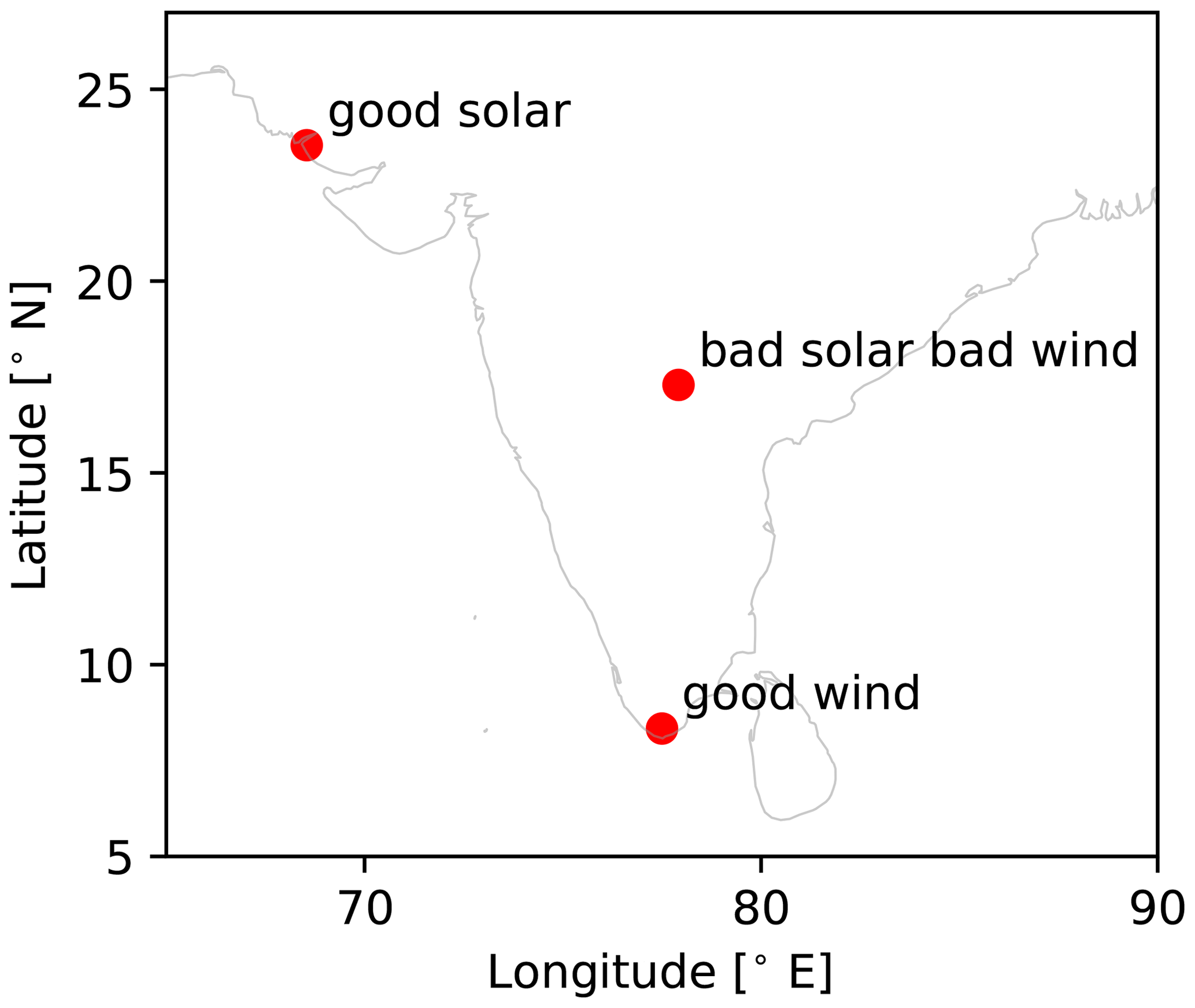
Figure 8Location of the three example sites.
Table 1Assumptions for the HPP sizing optimization with two scenarios for battery costs. O&M: operation and maintenance.
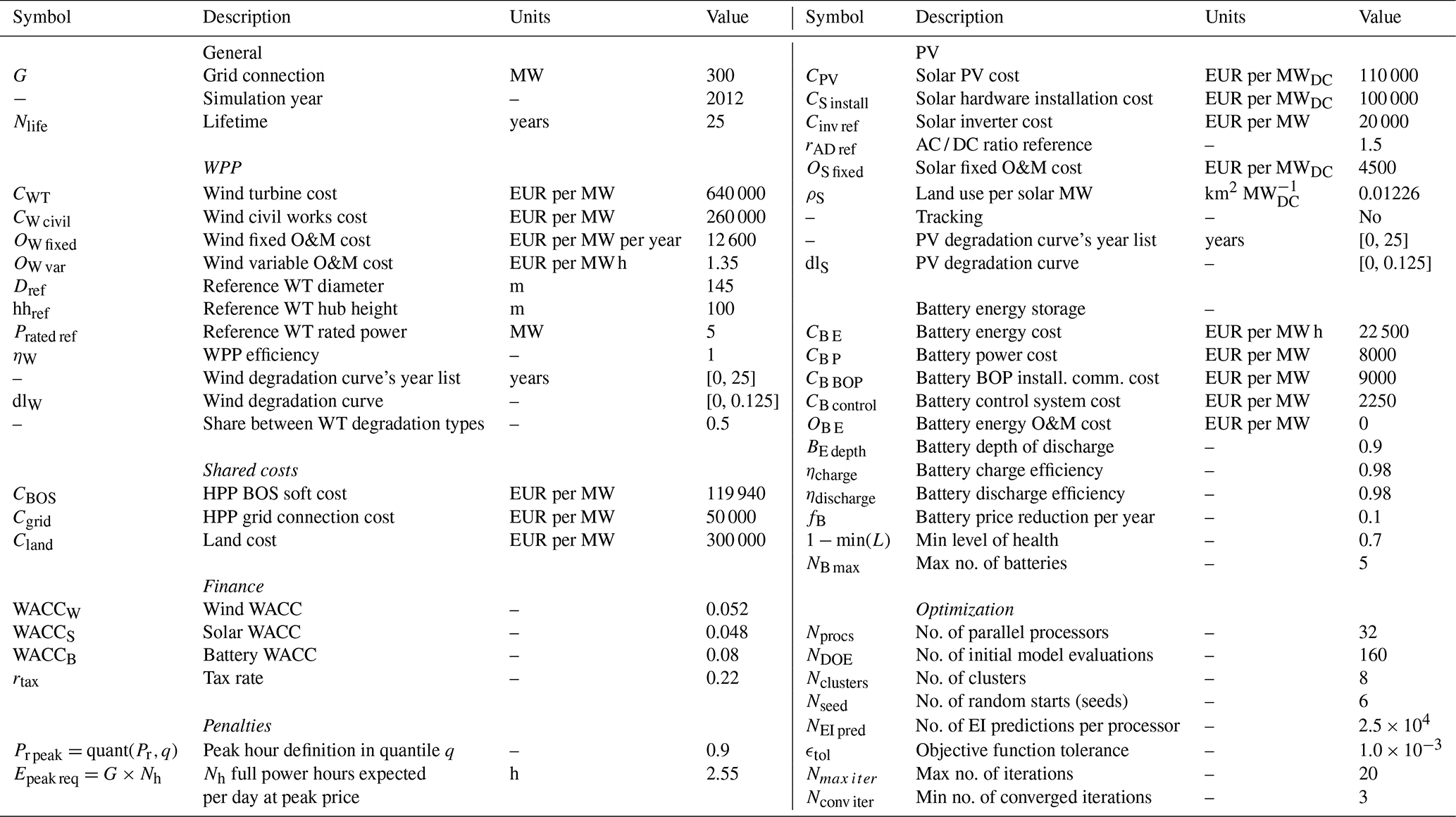
Three locations in India are selected as study cases (see Fig. 8). These locations are selected because they have a good balance between having good wind resources, good solar resources, or intermediate resources. The wind speed and irradiance statistics are presented in Fig. 9. A summary of costs, assumptions, and specifications used for this analysis is presented in Tables 1 and 2. The costs are taken from the Danish Energy Agency (DEA) Technology Catalogue (Danish Energy Agency, 2020), while the PV and wind degradation of 0.5 % yr−1 are taken from Theristis et al. (2023) and Hamilton et al. (2020). For each location, the optimization problem is executed based on two different (single) design objectives – LCoE and – in order to illustrate the benefits of HPP design based on revenue. Each optimization is executed with six multi-starts in order to ensure global optimality. Finally, we present a sensitivity analysis of the optimization results to varying all battery-related costs by applying a factor.
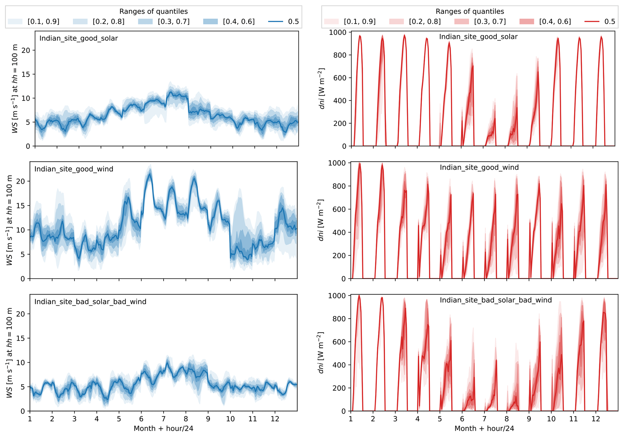
Figure 9Hourly statistics per month for wind speed and direct normal irradiance on the three locations.
The detailed results of the hybrid plant sizing optimization based on minimizing LCoE or on maximizing for the three different locations in India are presented in Table 3. It is observed that batteries are only installed for -based optimal sizing. This is an expected result as batteries add to the costs and do not increase the AEP, besides any curtailment reduction, and therefore do not reduce the LCoE. On -optimal plants, the optimizer tries to minimize the penalties by over-planting the generation and by introducing storage. Over-planting is a concept that has been proposed to increase revenue of WPPs when considering losses (Wolter et al., 2020). In general, the LCoE-based designs are single-generation technologies because the best-performing (lower-LCoE) energy source is prioritized; a low amount of over-planting is observed to compensate for the degradation over the lifetime. Because the LCoE does not account for the penalties, the LCoE-based designs produce negative business cases (NPV<0) for the sites with good solar and bad solar and bad wind. Note that llife in Table 3 represents the total penalties summed over the lifetime and can be twice as large as the total CAPEX on LCoE-based designs. AEcurt represents the mean annual energy curtailment and tends to be smaller than the AEP on all sites. The grid utilization factor, defined as the ratio between the mean HPP power and the grid connection (), better captures the capacity factor of an HPP, as it accounts for the energy sold to the grid. It can be seen that the grid utilization factor is larger for -based designs on the solar-driven sites, while it is slightly reduced on the site with good wind.
On the site with good solar, an HPP of PV and storage is obtained for the -based design with significant over-planting, while a single technology PV plant is obtained for the LCoE-based design. The PV panel orientation and rAD are very similar for both cases, but an increase in tilt indicates an effort to increase the generation closer to the morning peak price.
On the site with good wind, a single wind plant with minimal over-planting is obtained for the LCoE-based design, with high-rated power and a tall tower. A hybrid wind, PV, and storage plant with over-planting is selected for the -based design. At this plant, the turbines are smaller with lower towers and with additional generation produced by PV. The resulting battery power and energy rating are reduced compared to the other sites, which implies that the hybrid generation requires less energy shifting from non-peak to peak hours. On the contrary, this site uses three batteries instead of only two in the other locations. It is interesting to see that both designs at this location have similar final and LCoE values, highlighting that you can achieve similar objectives with multiple combinations of technologies.
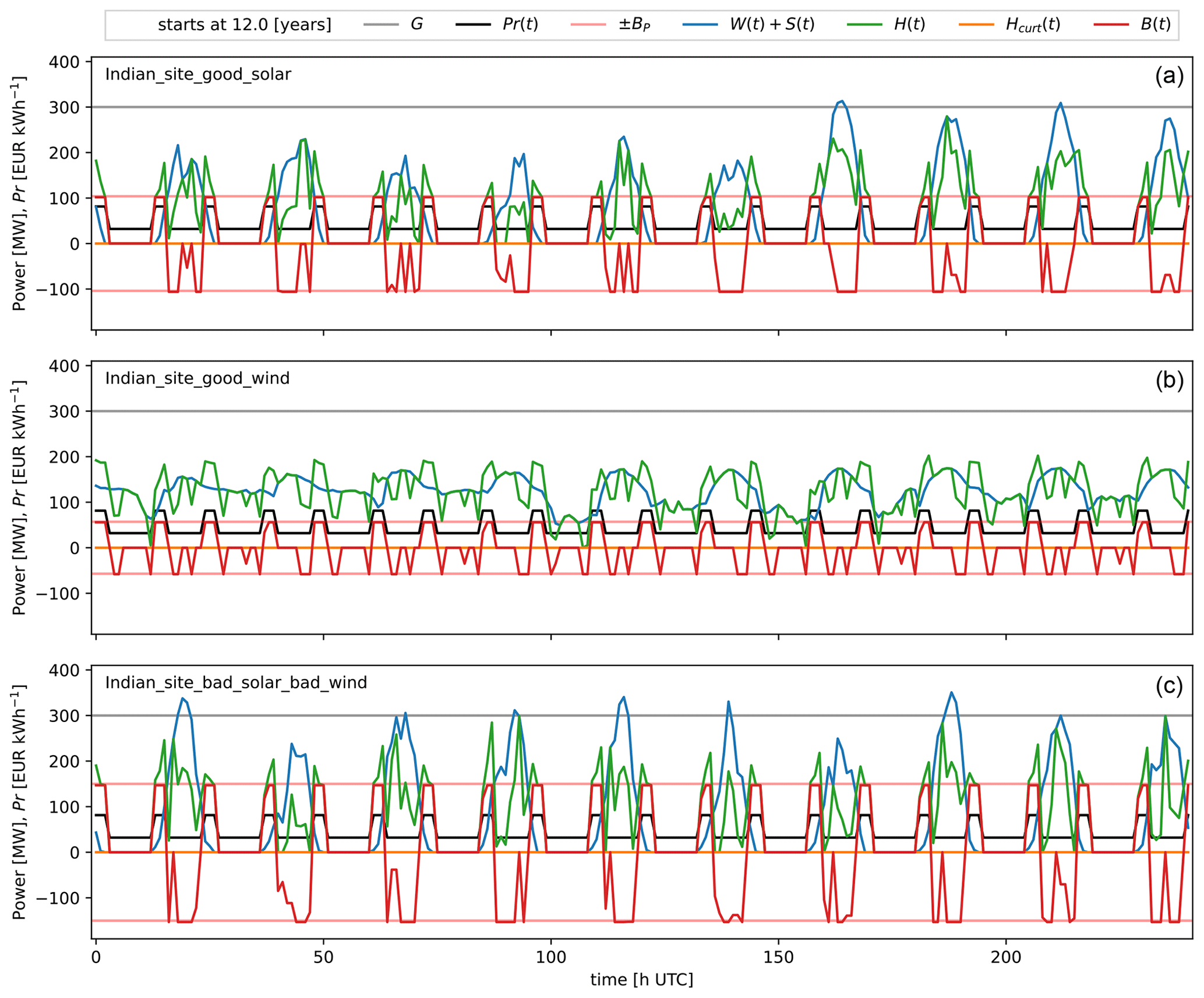
Figure 10Example of 10 d of operation on the 12th year for the -optimized HPPs at the following sites: (top) good solar, (center) good wind, and (bottom) bad solar and bad wind.
On the site with bad solar and bad wind, a PV plant with a storage plant is obtained for the -based design. Note that PV-only plants are, in general, over-planted (320 MW over 300 MW grid); the reason for this is to obtain a better AEP and GUF. An example period of operation of the -based HPPs for all sites is shown in Fig. 10.
Table 3HPP sizing optimization results in the example sites with respect and LCoE.
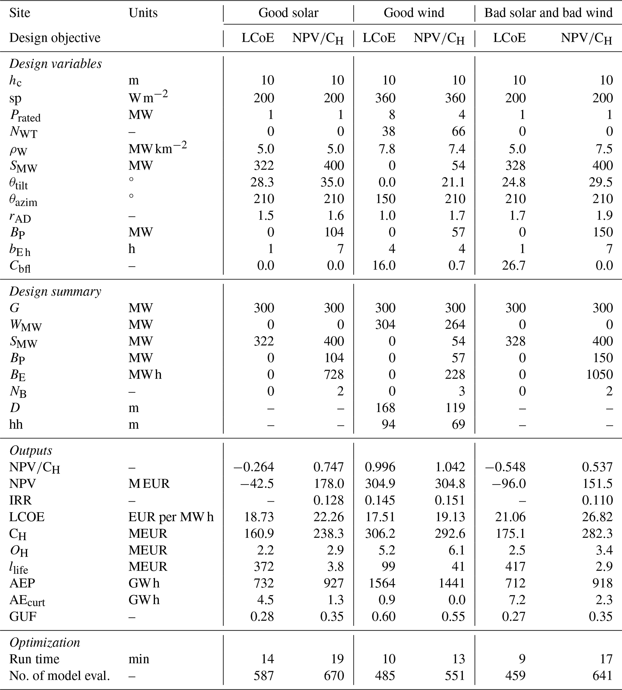
Figure 11 depicts the results of -based optimizations run with varying battery costs. Note that all the battery-related costs are scaled by a unique factor. It can be seen that the cost of batteries has a significant impact on the final HPP design and performance. The overall business case () is reduced when the batteries are more expensive for all sites. For the sites with good solar and bad solar and bad wind, the optimal HPP is very similar in terms of wind, solar, and the number of batteries. While on the site with good wind, batteries are not installed if they are 1.5 times more expensive; instead the amount of wind and PV over-planting increases to reduce the penalties and keep a similar business case. Finally, the optimizer decreases the power rating of the batteries when they are more expensive, but a small increase in the energy capacity is seen on the sites with good solar and bad solar and bad wind.
Hybrid power plants with storage are obtained across India with -based designs as a consequence of trying to mitigate the penalties of not reaching the expected energy generation at peak hours. Li-ion batteries are installed on sites that can not mitigate penalties by over-planting. The results show how changing from a LCoE- to -driven design allows the optimizer to over-dimension the generation and include storage to maximize the revenue by balancing the CAPEX, OPEX, power curtailment, and penalties. Hybrid plants, which include wind, solar, and battery, only occur on sites where the wind and solar generation complement each other to match the spot price signal (good wind).
Battery degradation plays an important role in HPP sizing as the additional costs of replacing the battery one or two times will change the financial viability of the project.
The sizing optimization prioritizes cheaper turbines for the -based HPP on the site with good wind, by selecting a lower hub height and lower-rated power.
The proposed nested-optimization approach ensures realistic HPP operation and at the same time allows for having non-linear sizing optimization. In the proposed framework, both EMS models are necessary since it is not computationally feasible to solve the internal EMS optimization for varying degradation states for the full lifetime within an outer sizing optimization. Instead, the rule-based long-term EMS is used to account for component degradation in a computationally efficient way. Hybrid power plants should be designed considering a realistic representation of the technologies, including their degradation.
The IRR is not defined when the NPV is negative, but such business cases occur on several HPPs evaluated during a sizing optimization and even on some LCoE-optimal HPPs. This illustrates why it is not possible to size HPP sites based on IRR, but instead, we propose the use of among other modified IRRs.
Future work will look into integrating stochastic optimization with internal operation optimization to have operation strategies that are robust to the forecast errors. Furthermore, HPP sizing optimization under cost and future spot price uncertainties is planned.
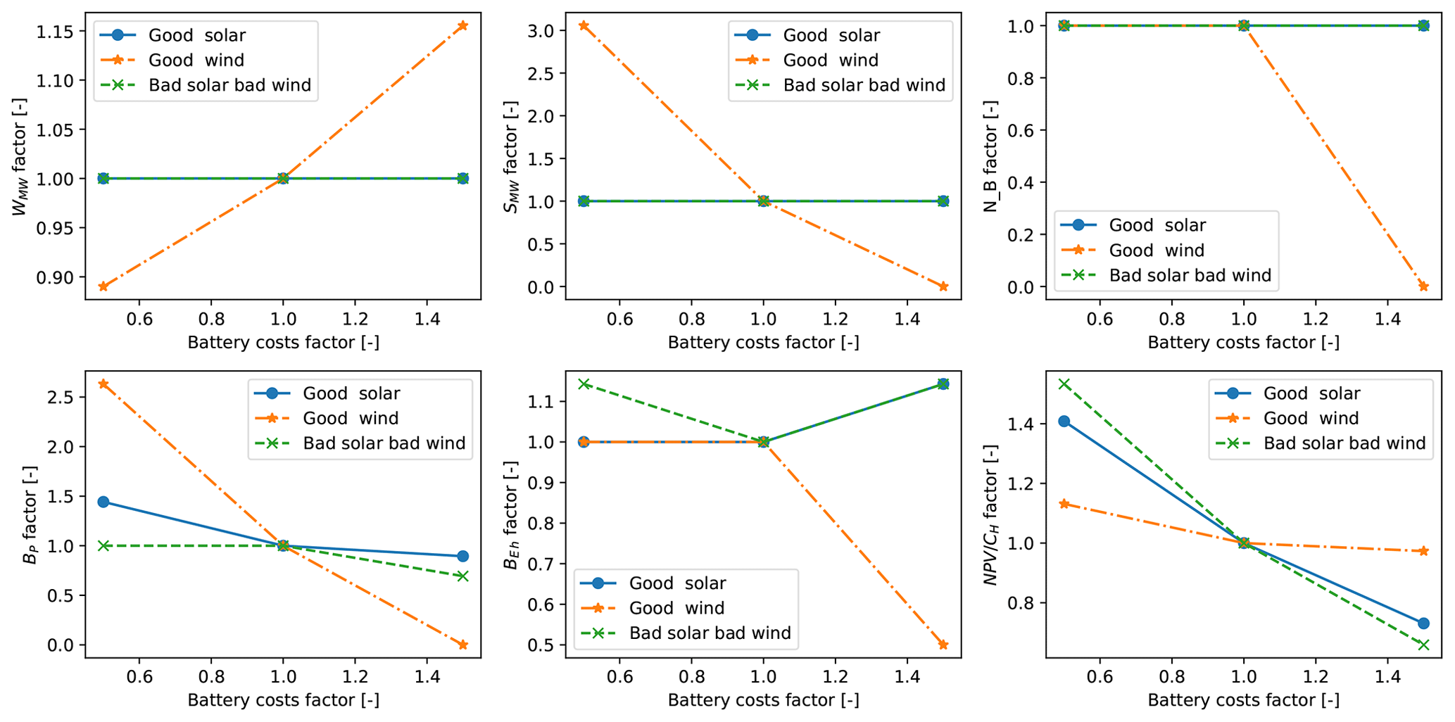
Figure 11Sensitivity of some key outputs for -optimal plants at the three locations when scaling all battery-related costs.
HyDesign is an open-source code for the design and control of a utility-scale hybrid power plant (HPP) based on wind and solar storage. The documentation and interactive examples are available at (https://topfarm.pages.windenergy.dtu.dk/hydesign/, DTU, 2024a); the input data including weather and price signals for the example Indian sites used in this article are available in the HyDesign repository as examples (https://gitlab.windenergy.dtu.dk/TOPFARM/hydesign, DTU, 2024b).
JPML is responsible for the model development, overall implementation, and the article. HH implemented the rule-based correction method. MFM contributed to the implementation of the parallel EGO algorithm. MG contributed to the improvement of the EMS formulation. RZ contributed to the initial implementation of the battery degradation model. KD provided funding and supervision. All authors contributed to the article.
The contact author has declared that none of the authors has any competing interests.
Publisher's note: Copernicus Publications remains neutral with regard to jurisdictional claims made in the text, published maps, institutional affiliations, or any other geographical representation in this paper. While Copernicus Publications makes every effort to include appropriate place names, the final responsibility lies with the authors.
Part of the research was performed within the REALISE project funded by EUDP (journal no. 64021-2049) and as part of the Indo-Danish project “HYBRIDize” (https://orbit.dtu.dk/en/projects/optimized-design-and-operation-of-hybrid-power-plant, last access: 1 February 2024) funded by the Innovationsfonden (Innovation Fund Denmark, IFD). Kaushik Das would also like to acknowledge the EUDP IEA Wind Task 50 project for supporting his hours used for contributing to the article.
This research has been supported by the EUDP-funded REALISE project (grant no. 64021-2049) and the IFD-funded HYBRIDize project.
This paper was edited by Jennifer King and reviewed by two anonymous referees.
Al-Lawati, R. A., Crespo-Vazquez, J. L., Faiz, T. I., Fang, X., and Noor-E-Alam, M.: Two-stage stochastic optimization frameworks to aid in decision-making under uncertainty for variable resource generators participating in a sequential energy market, Appl. Energ., 292, 116882, 2021. a
Astolfi, D., Pandit, R., Celesti, L., Lombardi, A., and Terzi, L.: SCADA data analysis for long-term wind turbine performance assessment: A case study, Sustainable Energy Technologies and Assessments, 52, 102357, https://doi.org/10.1016/j.seta.2022.102357, 2022. a
Bech, J. I., Hasager, C. B., and Bak, C.: Extending the life of wind turbine blade leading edges by reducing the tip speed during extreme precipitation events, Wind Energ. Sci., 3, 729–748, https://doi.org/10.5194/wes-3-729-2018, 2018. a
Bouhlel, M. A., Bartoli, N., Otsmane, A., and Morlier, J.: An improved approach for estimating the hyperparameters of the kriging model for high-dimensional problems through the partial least squares method, Math. Probl. Eng., 2016, 6723410, https://doi.org/10.1155/2016/6723410, 2016a. a
Bouhlel, M. A., Bartoli, N., Otsmane, A., and Morlier, J.: Improving kriging surrogates of high-dimensional design models by Partial Least Squares dimension reduction, Struct. Multidiscip. O., 53, 935–952, 2016b. a
Bouhlel, M. A., Hwang, J. T., Bartoli, N., Lafage, R., Morlier, J., and Martins, J. R. R. A.: A Python surrogate modeling framework with derivatives, Adv. Eng. Softw., 135, 102662, https://doi.org/10.1016/j.advengsoft.2019.03.005, 2019. a
Boyson, W. E., Galbraith, G. M., King, D. L., and Gonzalez, S.: Performance model for grid-connected photovoltaic inverters, OSTI.GOV, https://doi.org/10.2172/920449, 2007. a
Camargo, L. R. and Schmidt, J.: Simulation of multi-annual time series of solar photovoltaic power: Is the ERA5-land reanalysis the next big step?, Sustainable Energy Technologies and Assessments, 42, 100829, 2020. a
Danish Energy Agency: Technology Catalogues, https://ens.dk/en/our-services/projections-and-models/technology-data (last access: 1 February 2024), 2020. a
Das, K., Grapperon, A. L. T. P., Sørensen, P. E., and Hansen, A. D.: Optimal battery operation for revenue maximization of wind-storage hybrid power plant, Electr. Pow. Syst. Res., 189, 106631, https://doi.org/10.1016/j.epsr.2020.106631, 2020. a
Davies, J. A., Abdel-Wahab, M., and Mckay, D. C.: Estimating Solar Irradiation on Horizontal Surfaces, Int. J. Solar Energ., 2, 405–424, https://doi.org/10.1080/01425918408909940, 1984. a
Downing, S. D. and Socie, D.: Simple rainflow counting algorithms, Int. J. Fatigue, 4, 31–40, 1982. a
Dykes, K., King, J., DiOrio, N., King, R., Gevorgian, V., Corbus, D., Blair, N., Anderson, K., Stark, G., Turchi, C., and Moriarty, P.: Opportunities for Research and Development of Hybrid Power Plants, OSTI.GOV, https://doi.org/10.2172/1659803, 2020. a, b
DTU: Welcome to hydesign, https://topfarm.pages.windenergy.dtu.dk/hydesign/ (last access: 2 April 2024), 2024a. a
DTU: hydesign, https://gitlab.windenergy.dtu.dk/TOPFARM/hydesign (last access: 2 April 2024), 2024b. a
Dykes, K. L., Damiani, R. R., Graf, P. A., Scott, G. N., King, R. N., Guo, Y., Quick, J., Sethuraman, L., Veers, P. S., and Ning, A.: Wind turbine optimization with WISDEM, Tech. rep., National Renewable Energy Lab. (NREL), Golden, CO, USA, 2018. a
Elkan, C.: Using the triangle inequality to accelerate k-means, in: Proceedings of the 20th International Conference on Machine Learning (ICML-03), Washington, DC, USA, 147–153, https://cdn.aaai.org/ICML/2003/ICML03-022.pdf (last access: 2 April 2024), 2003. a
Gorman, W., Mills, A., Bolinger, M., Wiser, R., Singhal, N. G., Ela, E., and O'Shaughnessy, E.: Motivations and options for deploying hybrid generator-plus-battery projects within the bulk power system, Electricity Journal, 33, 106739, https://doi.org/10.1016/j.tej.2020.106739, 2020. a
Hamilton, S. D., Millstein, D., Bolinger, M., Wiser, R., and Jeong, S.: How does wind project performance change with age in the United States?, Joule, 4, 1004–1020, 2020. a, b
Hersbach, H., Bell, B., Berrisford, P., Hirahara, S., Horányi, A., Muñoz-Sabater, J., Nicolas, J., Peubey, C., Radu, R., Schepers, D., Simmons, A., Soci, C., Abdalla, S., Abellan, X., Balsamo, G., Bechtold, P., Biavati, G., Bidlot, J., Bonavita, M., De Chiara, G., Dahlgren, P., Dee, D., Diamantakis, M., Dragani, R., Flemming, J., Forbes, R., Fuentes, M., Geer, A., Haimberger, L., Healy, S., Hogan, R. J., Hólm, E., Janisková, M., Keeley, S., Laloyaux, P., Lopez, P., Lupu, C., Radnoti, G., de Rosnay, P., Rozum, I., Vamborg, F., Villaume, S., and Thépaut, J.-N.: The ERA5 global reanalysis, Q. J. Roy. Meteor. Soc., 146, 1999–2049, https://doi.org/10.1002/qj.3803, 2020. a
Holmgren, W. F., Hansen, C. W., and Mikofski, M. A.: pvlib python: a python package for modeling solar energy systems, Journal of Open Source Software, 3, 884, https://doi.org/10.21105/joss.00884, 2018. a
IEC: IEC 61400-1, Wind turbines – Part 1: Design requirements, https://webstore.iec.ch/publication/26423 (last access: 2 April 2024), 2017. a
Jia, X., Jin, C., Buzza, M., Wang, W., and Lee, J.: Wind turbine performance degradation assessment based on a novel similarity metric for machine performance curves, Renew. Energ., 99, 1191–1201, 2016. a
Jin, R., Chen, W., and Sudjianto, A.: An efficient algorithm for constructing optimal design of computer experiments, J. Stat. Plan. Infer., 134, 268–287, https://doi.org/10.1016/j.jspi.2004.02.014, 2005. a
Jones, D. R., Schonlau, M., and Welch, W. J.: Efficient global optimization of expensive black-box functions, J. Global Optim., 13, 455–492, 1998. a
Jordan, D. C., Deceglie, M. G., and Kurtz, S. R.: PV degradation methodology comparison—A basis for a standard, in: 2016 IEEE 43rd Photovoltaic Specialists Conference (PVSC), 5–10 June 2016, Portland, OR, USA 0273–0278, https://doi.org/10.1109/PVSC.2016.7749593, 2016. a
Kasten, F. and Young, A. T.: Revised optical air mass tables and approximation formula, Appl. Optics, 28, 4735–4738, 1989. a
Khaloie, H., Anvari-Moghaddam, A., Contreras, J., and Siano, P.: Risk-involved optimal operating strategy of a hybrid power generation company: A mixed interval-CVaR model, Energy, 232, 120975, https://doi.org/10.1016/j.energy.2021.120975, 2021a. a
Khaloie, H., Anvari-Moghaddam, A., Hatziargyriou, N., and Contreras, J.: Risk-constrained self-scheduling of a hybrid power plant considering interval-based intraday demand response exchange market prices, J. Clean. Prod., 282, 125344, https://doi.org/10.1016/j.jclepro.2020.125344, 2021b. a
Kratochvil, J. A., Boyson, W. E., and King, D. L.: Photovoltaic array performance model, OSTI.GOV, https://doi.org/10.2172/919131, 2004. a
López, J. C., Kolios, A., Wang, L., and Chiachio, M.: A wind turbine blade leading edge rain erosion computational framework, Renew. Energ., 203, 131–141, 2023. a, b
Maxwell, E. L.: A quasi-physical model for converting hourly global horizontal to direct normal insolation, Technical Report No. SERI/TR-215-3087, Solar Energy Research Institute, https://www.osti.gov/biblio/5987868 (last access: 2 April 2024), 1987. a
McKay, M. D., Beckman, R. J., and Conover, W. J.: A comparison of three methods for selecting values of input variables in the analysis of output from a computer code, Technometrics, 42, 55–61, 2000. a
Murcia, J. P., Koivisto, M. J., Luzia, G., Olsen, B. T., Hahmann, A. N., Sørensen, P. E., and Als, M.: Validation of European-scale simulated wind speed and wind generation time series, Appl. Energ., 305, 117794, 2022. a
Panthi, K. and Iungo, G. V.: Quantification of wind turbine energy loss due to leading-edge erosion through infrared-camera imaging, numerical simulations, and assessment against SCADA and meteorological data, Wind Energy, 26, 266–282, 2023. a
Pedersen, M. M., Meyer Forsting, A., van der Laan, P., Riva, R., Alcayaga Román, L. A., Criado Risco, J., Friis-Møller, M., Quick, J., Schøler Christiansen, J. P., Valotta Rodrigues, R., Olsen, B. T., and Réthoré, P.-E.: PyWake 2.5.0: An open-source wind farm simulation tool, https://gitlab.windenergy.dtu.dk/TOPFARM/PyWake (last access: 1 February 2024), 2023. a, b
Roux, É., Tillier, Y., Kraria, S., and Bouchard, P.-O.: An efficient parallel global optimization strategy based on Kriging properties suitable for material parameters identification, Archive of Mechanical Engineering, 169–195, https://doi.org/10.24425/ame.2020.131689, 2020. a
Safari, M., Morcrette, M., Teyssot, A., and Delacourt, C.: Multimodal physics-based aging model for life prediction of Li-ion batteries, J. Electrochem. Soc., 156, A145, 2008. a
Shi, Y., Xu, B., Tan, Y., and Zhang, B.: A convex cycle-based degradation model for battery energy storage planning and operation, in: 2018 Annual American Control Conference (ACC), IEEE, 27–29 June 2018, Milwaukee, WI, USA, 4590–4596, https://doi.org/10.23919/ACC.2018.8431814, 2018. a
Staffell, I. and Green, R.: How does wind farm performance decline with age?, Renew. Energ., 66, 775–786, 2014. a
Theristis, M., Livera, A., Jones, C. B., Makrides, G., Georghiou, G. E., and Stein, J. S.: Nonlinear photovoltaic degradation rates: Modeling and comparison against conventional methods, IEEE J. Photovolt., 10, 1112–1118, 2020. a
Theristis, M., Stein, J. S., Deline, C., Jordan, D., Robinson, C., Sekulic, W., Anderberg, A., Colvin, D. J., Walters, J., Seigneur, H., and King, B. H.: Onymous early-life performance degradation analysis of recent photovoltaic module technologies, Progress in Photovoltaics: Research and Applications, 31, 149–160, 2023. a, b
Tripp, C., Guittet, D., King, J., and Barker, A.: A simplified, efficient approach to hybrid wind and solar plant site optimization, Wind Energ. Sci., 7, 697–713, https://doi.org/10.5194/wes-7-697-2022, 2022. a
Vetter, J., Novák, P., Wagner, M. R., Veit, C., Möller, K.-C., Besenhard, J., Winter, M., Wohlfahrt-Mehrens, M., Vogler, C., and Hammouche, A.: Ageing mechanisms in lithium-ion batteries, J. Power Sources, 147, 269–281, 2005. a
Wang, Y., Zhao, H., and Li, P.: Optimal offering and operating strategies for Wind-Storage system participating in spot electricity markets with progressive stochastic-robust hybrid optimization model series, Math. Probl. Eng., 2019, 2142050, https://doi.org/10.1155/2019/2142050, 2019. a
Wolter, C., Klinge Jacobsen, H., Zeni, L., Rogdakis, G., and Cutululis, N. A.: Overplanting in offshore wind power plants in different regulatory regimes, WIREs Energy Environ., 9, e371, https://doi.org/10.1002/wene.371, 2020. a
Xu, B., Oudalov, A., Ulbig, A., Andersson, G., and Kirschen, D. S.: Modeling of lithium-ion battery degradation for cell life assessment, IEEE T. Smart Grid, 9, 1131–1140, 2016. a, b
Zong, H. and Porté-Agel, F.: A momentum-conserving wake superposition method for wind farm power prediction, J. Fluid Mech., 889, A8, https://doi.org/10.1017/jfm.2020.77, 2020. a