The near-wake development of a wind turbine operating in stalled conditions – Part 1: Assessment of numerical models

This study comprehensively investigates the near-wake development of a model wind turbine operating at a low tip-speed ratio in stalled conditions. In the present paper, part 1, different ways of representing the turbine, which include a full geometrical representation and modeling by means of the actuator line method, and different approaches for the modeling of turbulence are assessed. The simulation results are compared with particle image velocimetry (PIV) measurements from the MEXICO and New MEXICO experiments. A highly resolved numerical setup was created and a higher-order numerical scheme was applied to target an optimal resolution of the tip vortex development and the wakes of the blades. Besides the classical unsteady Reynolds-averaged methodology, a recently developed variant of the detached-eddy simulation (DES) was employed, which features robust shielding capabilities of the boundary layers and enhanced transition to a fully developed large-eddy simulation (LES) state. Two actuator line simulations were performed in which the aerodynamic forces were either evaluated by means of tabulated data or imposed from the averaged blade loads of the simulation with full blade geometry. The purpose is to distinguish between the effects of the force projection and the force calculation in the underlying blade-element method on the blade wake development. With the hybrid Reynolds-averaged Navier–Stokes (RANS)–LES approach and the geometrically fully resolved rotor blade, the details of the flow of the detached blade wake could be resolved. The prediction of the wake deficit also agreed very well with the experimental data. Furthermore, the strength and size of the blade tip vortices were correctly predicted. With the linear unsteady Reynolds-averaged Navier–Stokes (URANS) model, the wake deficit could also be described correctly, yet the size of the tip vortices was massively overestimated. The actuator line method, when fed with forces from the fully resolved simulation, provides very similar results in terms of wake deficit and tip vortices to its fully resolved parent simulation. However, using uncorrected two-dimensional polars shows significant deviations in the wake topology of the inner blade region. This shows that the application in such flow conditions requires models for rotational augmentation. In part 2 of the study, to be published in another paper, the development and the dynamics of the early tip vortex formation are detailed.

1 Introduction

During the total optimization of the levelized cost of energy, the turbines in the wind farms have to be placed ever closer to each other so that distances of the order of 2–3 rotor diameters prevail in some wind directions. This means that the turbines are increasingly being placed in the near wake rather than the far wake. Compared to the far wake, which is mainly characterized by isotropic turbulence and where the influence of the detailed rotor aerodynamics plays a subordinate role, in the near wake (one to two rotor diameters), the effects of blade circulation and the transient events of the blade passage govern the unsteadiness in the wake. In particular, the tip and hub vortices characterize the flow topology of the wake. In addition, viscous effects like flow separation can also become relevant under certain operating conditions. To provide proof of the dynamic loads in such wake scenarios over the entire machine lifetime of 20 years, turbine manufacturers and park developers utilize engineering wake models (Frandsen et al., 2006; Jensen, 1983) and the dynamic wake meandering model (Larsen et al., 2007). These models only incorporate a very simplified model representing the turbine and its operation. They are only valid in the far wake and exhibit inaccuracies in the near wake.

Therefore, it is essential to understand, improve and further develop engineering models for the near wake. The starting point is to deepen the knowledge of the underlying physics and its simulative modeling. This is what this study aims to contribute to. Computational fluid dynamics (CFD) is applied with different levels of model fidelity to study the physical effects in the wake and to learn the limits of the respective method.

The test case at hand is the MEXICO model wind turbine operating in off-design conditions at a low tip-speed ratio in which the rotor is exposed to stall. The unsteady flow phenomena involved here are particularly challenging to predict for flow simulation in general. In order to assess different numerical models regarding the wake physics in such conditions, two different methods are applied to represent the rotor. These are, first, the geometrically fully resolved approach and, second, the actuator line (ACL) method (Sorensen and Shen, 2002). The latter promises significant computational time-saving compared to the full-resolution simulation, since both the spatial and the temporal resolution can be adapted to the chord of the blade instead of requiring the details of viscous boundary layers to be resolved. The method is applied in two different modeling depths. First, it is applied in a “forced” mode, where the averaged forces from the full-resolution simulation are injected at the rotating line. This is to examine to what extent the same circulation and wake properties can be achieved as with the full-resolution method, having the same averaged aerodynamic forces at the blade in both cases. In a second step, the ACL is used classically with internal force calculation, with which the quality of the blade-element method (BEM) for detached flows is to be verified. Regarding both modeling approaches, scale-resolving simulation techniques are applied and compared to classical Reynolds-averaged Navier–Stokes (RANS) turbulence modeling in order to expose the differences in the predicted wake topology.

1.1 Previous experimental and computational studies on the near wake

Experimental studies on the near wakes have mostly been conducted in controlled conditions of wind tunnels. In wind tunnels, data acquisition by means of particle image velocimetry (PIV) or hot-wire anemometry is easy compared to velocity measurements in the field. Moreover, the inflow conditions are well known and controlled, both of which make this type of testing suitable for the validation of numerical simulations. On the other hand, there is the drawback of scaling effects that result in relatively low Reynolds numbers and turbine designs that differ from modern multi-megawatt machines. Therefore, wind tunnel experiments based on small-scale or miniature turbines (Chamorro and Porté-Agel, 2009, 2010; Bottasso et al., 2014; Wang et al., 2021) typically focus on the effects of the atmospheric boundary layer, like shear, turbulence and stratification, on the turbines' wakes. As discussed in Wang et al. (2021), the wakes of the scaled turbine with the real full-scale machine agree well in the far wake beyond 4 rotor diameters in terms of wake deficit and turbulence statistics. The inconsistencies in the near wake are caused by differences in swirl and circulation distribution, as well as neglecting the effect of rotational augmentation.

Experiments with respect to the near wake of model wind turbines have been conducted by numerous research groups (Grant and Parkin, 2000; Ebert and Wood, 1999, 2001; Snel et al., 2007; Boorsma et al., 2014; Dobrev et al., 2008; Krogstad and Eriksen, 2013; Bartl and Sætran, 2017; Mühle et al., 2018; Micallef, 2012; Bastankhah and Porté-Agel, 2017; Okulov and Sørensen, 2007). The velocity deficits of the rotor blades a few chord lengths downstream of the blade were measured for example by Ebert and Wood (2001), Schepers and Snel (2007), and Micallef (2012). With that, a characterization of the induction effects of the blade passage in the very near field of the blade could be performed.

The importance of tip vortices in the evolution and collapse of the wake has been a further key focus in research during experiments and numerical analyses. The vortex roll-up process directly around the blade tip surface was investigated by Micallef et al. (2014). They found in PIV investigations on the Delft research turbine as well as by analyzing the data of the MEXICO turbine (Schepers and Snel, 2007) that the tip vortex stays inward of the blade tip at the early stages before any wake expansion sets in. The vortex propagation in the rotor wake of the aforementioned MEXICO turbine was extensively studied within the first MEXICO campaign in 2007 (Schepers and Snel, 2007). The tip vortices were tracked with the PIV technique on laser sheets placed along the expected vortex trajectories in the wake for each operational point of the turbine. These ranged from a turbulent wake state over the optimum tip-speed ratio to a high-wind-speed case in the stalled regime, for both axial and yawed inflow. In the Mexnext projects (Schepers et al., 2012; Boorsma et al., 2018), the University of Stuttgart processed the PIV data and extracted the following vortex properties: vortex position, strength (circulation) and size. The data were used to compare different CFD solvers and a free vortex code. In numerical studies using CFD, the tip vortex sizes were typically overpredicted compared to experiments. In the results of Schulz et al. (2016), who used unsteady Reynolds-averaged Navier–Stokes (URANS) simulations and a second-order convection scheme (Jameson et al., 1981) on a grid resolution equivalent to ≈16 % tip chord, the core radius was overestimated by a factor of 5. In the simulations of Nilsson et al. (2015), who employed the ACL method in a large-eddy simulation (LES) framework and a QUICK scheme on a grid resolution in the tip region equivalent to ≈20 % tip chord, the core radius was overestimated by approximately the same amount. Meister (2015) employed a vortex refinement mesh together with a higher-order WENO scheme (Jiang and Shu, 1996) with URANS, reducing the overprediction to a factor between 3 and 4. In the studies of Carrión et al. (2014, 2015), the low-Mach-number adapted Roe scheme (Rieper, 2011) was adopted together with URANS on a wake resolution equivalent to ≈6.5 % tip chord in order to reduce dissipation of compressible schemes at low Mach numbers. In their studies, the vortex core size was overpredicted by a factor of around 3 . Other parameters, such as vortex position, as well as integrated vortex circulation were accurately predicted by the aforementioned studies. Here, the determination of the load distribution on the rotor blade is evidently sufficient to correctly reflect the thrust and thus the wake induction and expansion as well as the circulation of the tailing tip vortices.

Further investigations on the tip vortex positions and the effect of vortex wandering were reported in Bailey and Tavoularis (2008) and Dobrev et al. (2008). These factors are important for understanding the instability mechanisms that eventually lead to vortex breakdown and mark the end of the near-wake region. Using PIV measurements and conditional averaging, Bailey and Tavoularis (2008) and Dobrev et al. (2008) separated the mean field from the vortex wandering and were able to map the variance of the vortex position. The vortex wandering was also evaluated in the study of Sherry et al. (2013), who investigated the wake of the Tjareborg wind turbine in a water tunnel at different tip-speed ratios. They found higher standard deviations of the vortex wandering for lower tip-speed ratios. The phenomenon of vortex wandering has recently also been extracted for the larger Berlin Research Turbine (BeRT) of the Technische Universität Berlin by Soto-Valle et al. (2022). Theoretical studies on the instability mechanisms leading to vortex breakdown were conducted by Ivanell et al. (2010), Sarmast et al. (2014) and Kleine et al. (2022) using ACL simulations and controlled perturbations. By means of modal analyses, the authors found the amplification of waves traveling along the vortex spiral that trigger the mutual inductance instability of the tip vortices.

The formation and development of the root vortex were investigated in the experimental study of Akay (2016) with PIV measurements, from which a three-dimensional reconstruction of the flow field was derived (Micallef, 2012; Akay, 2016). The study of Akay (2016) investigated the velocity and vorticity field with special attention given to the root vortex and related it to the spanwise flow around the blade. This test case was numerically studied by Herráez et al. (2016). In their study using the RANS approach, they investigated the formation of the root vortex in the very inner blade sections by comparing the velocity fields close to the blade surface with measured PIV data. They found overall good agreement with the velocity components already 10 mm above the blade surface, suggesting that for design conditions the RANS approach correctly captures the vortex roll-up mechanism.

Wind tunnel experiments for validating aerodynamic simulation tools were conducted within the blind test campaigns that were organized at the Norwegian University of Science and Technology (NTNU) (Krogstad and Eriksen, 2013; Bartl and Sætran, 2017; Mühle et al., 2018). In these experiments the complexity was increased from campaign to campaign, starting with a single wind turbine at uniform inflow, then adding wind shear and turbulence, and ending with yawed conditions and wake interaction. In the comparison of the numerical models with measurements, it turned out that a full-turbine representation in conjunction with detached-eddy simulations produced superior results, especially in highly complex flow situations such as yawed and partial wake situations, with respect to the velocity and turbulence field compared to RANS and actuator disk approaches. Actuator line simulations presented in Mühle et al. (2018) using experimental airfoil data and high grid resolution in combination with LES performed similarly well to the geometrically fully resolved improved delayed DES (IDDES) simulation.

The experimental results of the MEXICO and New MEXICO experiments were utilized as validation for a large number of numerical studies and were collected in Boorsma et al. (2018). The computational approaches ranged from lifting-line codes (Grasso et al., 2011) and actuator disk and actuator line methods (Sarmast et al., 2016; Nilsson et al., 2015) to full-turbine representations, which were simulated with the RANS (Lutz et al., 2011; Meister, 2015; Schulz et al., 2016; Bechmann et al., 2011; Sørensen et al., 2016; Carrión et al., 2014) and hybrid RANS–LES methods (Weihing et al., 2016) and more recently also with the Lattice–Boltzmann method (Li et al., 2021). As summarized by Boorsma et al. (2018), CFD simulations led to superior results in complex situations such as in stalled conditions but also to larger scattering among the different contributions. This implies that careful selection of the numerical input parameters, models and grid resolution is essential to achieve accurate predictions for the simulation problem at hand.

In order to evaluate the turbine modeling approach within a single numerical framework, Troldborg et al. (2015) compared the near wake of actuator disk and line simulations with blade-resolved simulations for the NREL 5 MW reference turbine in uniform and non-sheared turbulent inflow using both the RANS and the DES method. In the near wake, up to 1 diameter downstream of rotor, all three approaches resulted in very similar mean velocity profiles. However, the velocity fluctuations induced by the tip vortices were predicted to be lower in the ACL simulations and were by nature absent in the actuator disk results. In the transition from the near wake to the far wake, the breakdown of the tip vortices was predicted far too late in the actuator-type simulations. In turbulent inflow, the large-scale disturbances imposed by the ambient turbulence led to a very comparable breakdown mechanism of the wake in all three simulations and accordingly to very similar velocity and turbulence profiles. However, in the near wake at 1 rotor diameter into the wake, the actuator line method had the tendency of predicting higher velocity fluctuations in the hub region but larger fluctuations in the tip region compared to the fully resolved simulation. Good agreement between actuator line and fully resolved simulations under turbulent inflow was also found in the study (Weihing et al., 2017), where the ACL was compared to fully resolved simulations at high-turbulence ambient inflow in complex terrain and a lower-turbulence environment representative of offshore conditions. In both cases very similar wake topologies and breakdown phenomena could be observed, which lead to good agreement in the velocity and turbulence profiles, already in the near-wake region. More recently, Hodgson et al. (2022) compared ACL and blade-resolved simulations with the measurements gained in the DanAero experiment (Bak et al., 2010) for the NM80 turbine for axial and yawed inflow conditions. They employed the ACL coupled to the Flex5 solver to also capture aeroelastic effects like blade torsion and deflections. In the outer blade region, the loads were predicted to be lower than in the fully resolved simulations but were closer to the experimental data. The wake pattern and profiles were predicted similarly in the turbulent inflow cases for both approaches, despite the ACL being run on a coarser grid which dissipated the discrete tip vortices rather quickly.

1.2 Objectives and outline

The following objectives are addressed in part 1 of the study in the present paper:

1. It is assessed whether scale-resolving simulation methods yield improved predictions of the near-wake field for a turbine operating in stalled conditions with respect to the wake deficit and the tip vortex propagation.

2. It is examined whether the ACL method can be applied to stalled operation and how accurate the predictions are compared to fully resolved simulations and PIV experiments.

3. The influence of the force determination in the ACL method on the wake is investigated. The aim is to examine how forces from uncorrected two-dimensional polars affect the wake topology compared to forces inherited from a three-dimensional rotor simulation.

In part 2 of the study, to be published in another article, the formation process of the tip vortex and the development of secondary vortex structures will be investigated in detail.

The next section describes the experimental test case of the MEXICO turbine and the operating conditions. This is followed by information on the flow solver and the numerical modeling in Sect. 3 and on the employed computational setups in Sect. 4. The results are presented in Sect. 5, starting with the wake in the vicinity of the blade, then the rotor wake and finally the evolution of the tip vortices. The main conclusions are summarized in Sect. 6.

2 Test case

The MEXICO model wind turbine was experimentally studied in the large low-speed facility (LLF) of the Deutsch-Niederländische Windkanäle (German-Dutch Wind Tunnels, DNW) within two test campaigns. The first campaign took place in 2006 (Snel et al., 2007) and is referred to as the MEXICO campaign. In 2014 a second campaign was conducted with the same wind tunnel model, which is called the New MEXICO experiment (Boorsma and Schepers, 2015).

In principle, the basic test setup was the same in both campaigns. The arrangement is sketched in Fig. 1. The tunnel was operated in an open-jet mode with a contractor equipped with Seifert wings at the lip and a collector, resulting in a cross section of 9.5×9.5 m². The MEXICO model was mounted on a test rig, connected to the floor of the hall by the external balance.

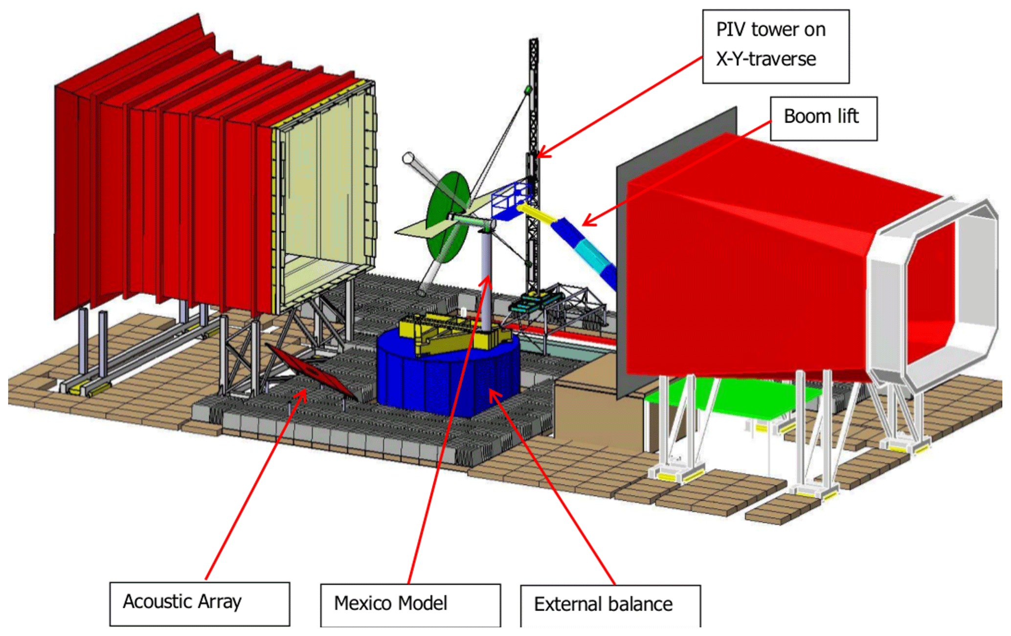
Figure 1 Sketch of the MEXICO test setup in the LLF (DNW) (Philipsen et al., 2014) (courtesy of Gerard Schepers, personal communication, 2021).

The PIV system was mounted on a tower located outside of the cross section and which enabled traversing in the horizontal plane. The camera arrangement was stereoscopic in order to obtain three velocity components in a two-dimensional slice. This slice lies in the horizontal (x–y) plane at hub height, as outlined in Fig. 1. The placement and number of the PIV sheets, as well as the phase angle relative to the rotor blade at which the snapshots were taken, varied depending on the evaluation and are detailed separately in their respective sections.

The MEXICO model turbine comprises three blades with a radius of 2.25 m, the tower and the nacelle. The latter includes the hub, which is a rotating ring located downstream of the non-rotating “spinner” and houses the generator in the rear part. The tower is located 2.13 m downstream of the rotor plane and has a diameter of 0.51 m. The blades of the model are instrumented with Kulite pressure sensors distributed over the five radial sections $r/R=\mathrm{0.25}$, 0.35, 0.60, 0.82 and 0.92.

The blade is composed of three different airfoils. The DU91-w2-250 is installed in the root region ($\mathrm{0.2}\le r/R\le \mathrm{0.44}$), the Risø-A1-21 in the mid-region ($\mathrm{0.55}\le r/R\le \mathrm{0.65}$) and the NACA 64-418 in the outboard section ($r/R>\mathrm{0.74}$). The shape of the blade tip is an ellipsoid. In the transition zones, the shape of the blade is linearly blended between the different airfoils. The chord and twist distributions, as well as the sectional Reynolds and Mach numbers, are shown in Fig. 2. The maximum tip speed of around 100 m s⁻¹ and the chord distribution were elaborated to maximize the Reynolds number while keeping the Mach number reasonably low. The Reynolds number is relatively constant over the radius and varies between 0.48 and 0.64 M. The Mach number, which is estimated from the kinematic inflow velocity, increases linearly and reaches a maximum value of around 0.3 at the blade tip. Compared to modern full-scale turbines, the Reynolds numbers are still more than 1 order of magnitude lower, whereas the Mach number is already slightly above. With a lower Reynolds number, the area of separation and its resolved structures are expected to be relatively larger compared to full-scale turbines. Additionally, a clear effect of compressibility can be expected, namely an increasing adverse pressure gradient and, therefore, an earlier separation than at full scale.

Figure 2 Radial distributions of the airfoil chord, twist angle, chord Reynolds number and inflow Mach number. The grey patches indicate the locations of the different airfoil types.

In contrast to the former MEXICO experiments (Schepers and Snel, 2007), where zig-zag tapes were applied over the entire blade radius, in the New MEXICO experiments, tripping was only applied to the inner rotor sections $\left(\frac{r}{R}<\mathrm{0.7}\right)$ (Boorsma and Schepers, 2015). For the outer rotor portion $\left(\frac{r}{R}>\mathrm{0.7}\right)$, clean conditions allow for natural laminar to turbulent transition of the boundary layer.

2.1 Operational conditions of the reference cases

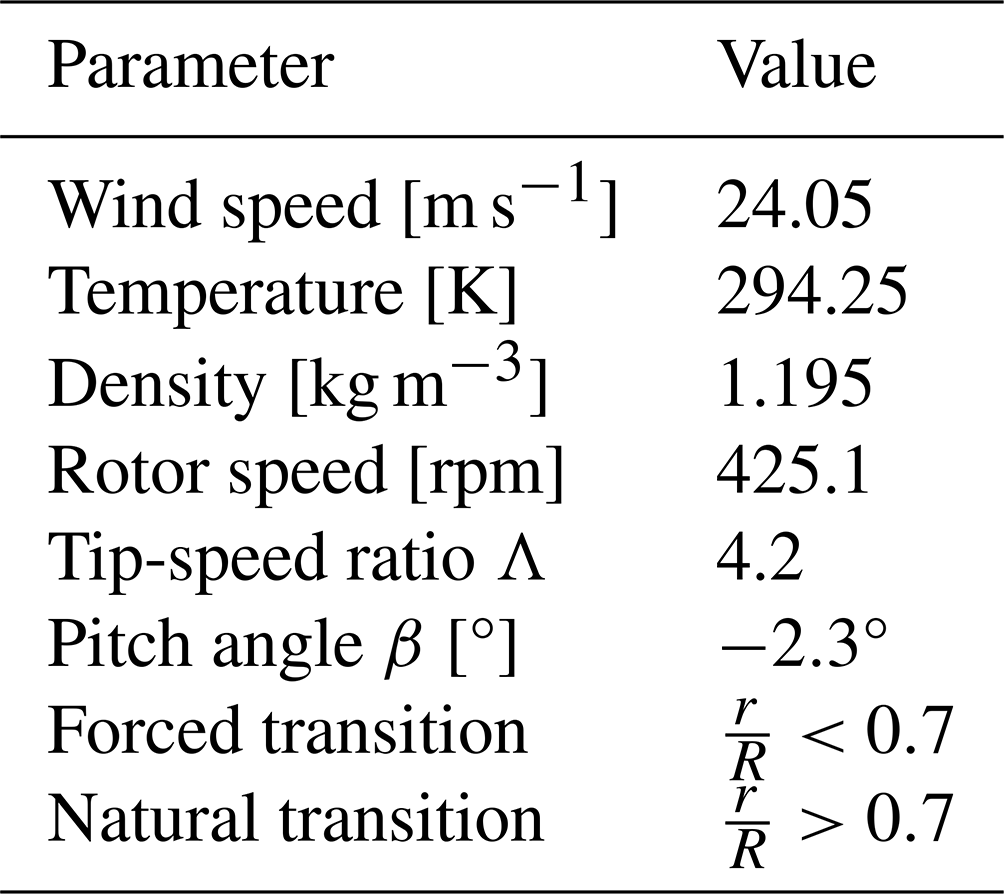
The reference case for the simulations presented is an off-design case at low tip-speed ratio. The pitch settings cause flow separation along the entire blade radius. The operation point is taken from Boorsma and Schepers (2017) and summarized in Table 1.

Table 1 Operational conditions for the MEXICO test cases in axial inflow.

It could be argued that such an off-design case has no practical relevance, since the turbine is supposed to operate outside of any stall issues. However, it is precisely the challenging flow patterns where CFD is applied in industry and where differences can be expected compared to engineering models. It is therefore highly important to thoroughly assess the accuracy and the best practices of CFD, especially with regard to evolving methods such as scale-resolving simulation techniques. This test case offers an excellent data basis with which the wake behavior and, in particular, the blade tip vortices can be analyzed in detail.

3 Flow solver and turbulence modeling

The simulations were performed with the block-structured, compressible flow solver FLOWer. The code was developed by the German Aerospace Center (DLR) (Kroll et al., 2000) and has undergone continuous development at the Institute of Aerodynamics and Gas Dynamics (IAG), facilitating the understanding of multidisciplinary flow phenomena of wind turbines. Relevant extensions for the present study are the higher-order numerical methods (Kowarsch et al., 2013), scale-resolving simulation techniques (Weihing et al., 2016, 2020) and the actuator line method (Weihing et al., 2017; Bühler et al., 2018; Cormier et al., 2021).

Two turbulence modeling approaches are investigated within the present simulations. The first is the unsteady RANS method based on the shear stress transport (SST) turbulence model (Menter, 1994). The location of laminar to turbulent transition is predicted using the amplification factor model of Coder (2014), which is coupled to the turbulence model by a transport equation of the intermittency variable, similar to the approach taken by Menter et al. (2015). The amplification model is based on elements of linear stability theory (Drela and Giles, 1987) and requires the specification of a critical amplification factor N_crit, which is set to 9 in the present study. Note that the transition model was zonally deactivated in the regions that are affected by the zig-zag tape. Thus, it is deactivated in the radial region $\frac{r}{R}<\mathrm{0.7}$, where we have a zig-zag tape but only downstream of it in the chordwise direction (10 % chord on suction and pressure side). The second approach is a recently developed variant (Weihing et al., 2020) of the detached-eddy simulation (DES). The main goal of DES is to treat the boundary layers in the RANS mode while resolving the separated flow structures in a LES-like behavior. In DES97 (Spalart, 1997) and also in Delayed DES (Spalart et al., 2006), it was observed that the LES domain may invade the boundary layer once the grid is refined. When this happens, the modeled stresses are reduced. Eventually, this leads to so-called grid-induced separation in flows with adverse pressure gradients. In the recently developed variant (Weihing et al., 2020) used in the present study, the interfaces between the RANS and LES domains are estimated based on a localized version of the Bernoulli equation. Therefore, the method is called BDES. It identifies the presence of resolved turbulence using a shear layer detector and the σ velocity gradient operator of Nicoud et al. (2011). It should be noted that, due to the presence of the local velocity within the Bernoulli equation, the method is not Galilean invariant. To overcome this problem, the velocities in the boundary layer and the freestream state need to be transformed relative to the considered wall. In the code, this is realized by subtracting the local velocities stemming from rigid-body motions and grid deformations from the values of the inertial system. This shielding method has proven to be very robust against grid-induced separation effects even under asymptotic grid refinement and adverse pressure gradients and has been successfully implemented and applied to separated flows in other solvers (Fuchs and Mockett, 2020; Ehrle et al., 2022). Furthermore, the velocity gradient operator within the turbulence model is replaced by the σ operator, once it is in LES mode (Mockett et al., 2015). Together with a filter width ${\mathrm{\Delta }}_{\stackrel{\mathrm{̃}}{\mathit{\omega }}}$, this reduces the eddy viscosity in areas of pure shear and solid rotation and thereby yields a faster development of the hybrid model towards a mature LES flow field. It should be noted that the LES model is only activated once the transition model is effectively in turbulent mode in order to prevent an unconstrained balance of production and destruction terms in the turbulence model.

Regarding the convection schemes, the inviscid fluxes are approximated by the higher-order WENO scheme of Martín et al. (2006), implemented with four-point stencils. The scheme features its optimal weights such that maximum bandwidth resolution is achieved rather than pure minimization of the truncation error. The viscous fluxes were approximated by central differences. Time integration is performed by explicit multi-stage Runge–Kutta schemes. A second-order implicit dual time-stepping algorithm according to Jameson (1991) is employed for time-accurate computations.

Moreover, the ACL approach (Sorensen and Shen, 2002; Mikkelsen, 2003) is used to include the effects of the blade aerodynamic forces as momentum sources in the Navier–Stokes equations. The two-dimensional aerodynamic forces at each blade element are distributed over the neighboring computational cells using a Gaussian function. In the current implementation, the loads can either be computed from the local flow field properties and tabulated airfoil data, in alignment with the original formulation, or be forced as a steady blade loading from an external radial force distribution. Further details on the ACL are found in Sect. 4.2.

4 Computational setup

Based on the experience gained during the Mexnext projects, a computational setup based on a one-third model was created. The impact of the tower, which is located almost 1 rotor radius downstream, was considered to be subordinate regarding the loads and near-wake behavior in uniform conditions. The numerical representation of the wind tunnel geometry was not considered, as the study of Réthoré et al. (2011) showed negligible influence on the velocity field upstream of the rotor, which can therefore be assumed uniform. Moreover, the wake development is not substantially affected by the tunnel environment.

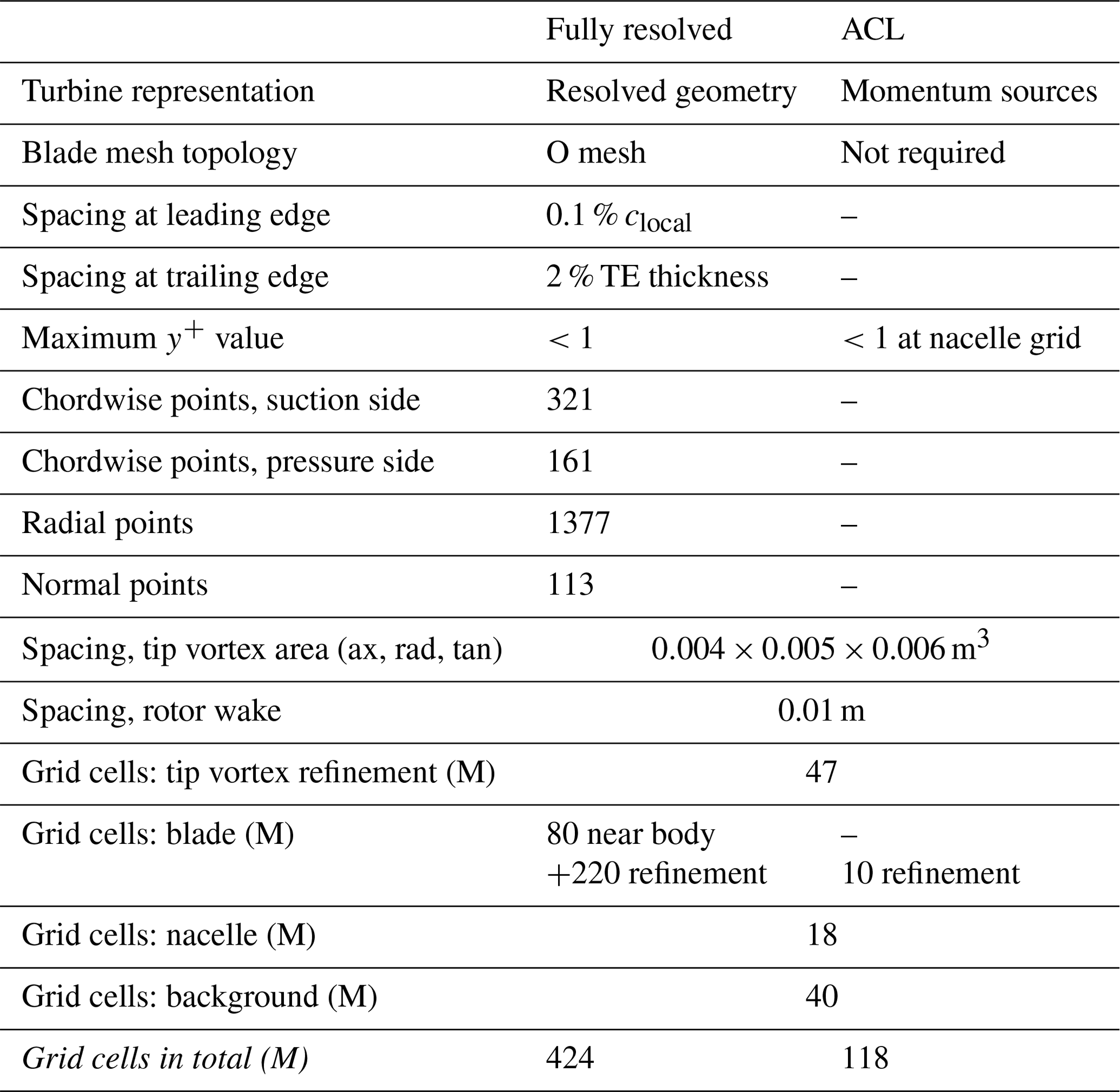
4.1 Grids

The grid used to resolve the flow field in the vicinity of the rotor blade consists of four parts, which are sketched in Fig. 3: the near-body grid covers the attached and separated boundary layers and extends around one-quarter of the chord from the blade surface. It is embedded into a Cartesian background grid with hanging nodes that refines the separated wake region and rotates with the blade. A tip cap closes the blade mesh and is required for topological reasons. At the root, a blade-connector grid is used to enable pitching of the cylindrical root relative to the nacelle. The near-body grid is constructed in an O-type topology, which was created by hyperbolic extrusion. The grid spacings, which are summarized in Table 2, were specified according to the recommendations of American Institute of Aeronautics and Astronautics's (AIAA) drag prediction workshop for aircraft wings (Vassberg et al., 2008). To keep the number of cells manageable, the number of grid points was higher on the suction side (321 nodes) than on the pressure side (161 nodes). However, this required the construction of a cap mesh at the blade tip to close the grid. In the radial direction, the grid spacing is adapted to 1 % of the local chord. The near-body grid is embedded into a Cartesian background mesh which rotates with the blade and serves as a refinement of the separated airfoil wake. It is extended around 1.5 local chord lengths downstream, and the spacing is around 0.7 % c_mean.

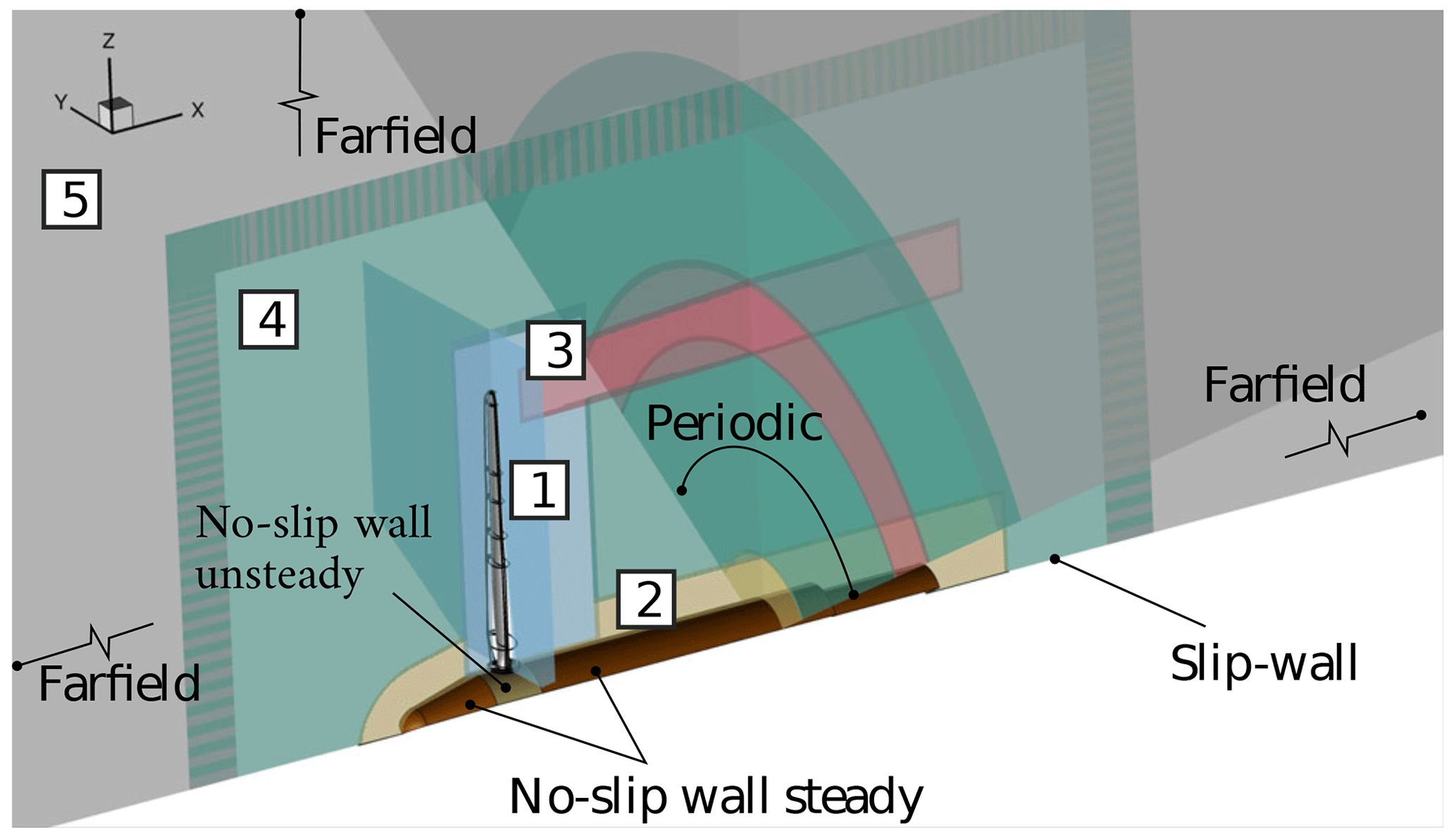
Figure 3 Overlapping grid structures and boundary conditions of the simulation setup for the MEXICO one-third model wind turbine.

Table 2 Cell spacings and grid information.

The grid of the nacelle, labeled 2 in Fig. 3, consists of a one-third periodic surface segment, which, however, does not use a singular line due to problems of that boundary condition with the WENO scheme. Instead, a very small angular segment is created near the axial center that is treated as a slip wall. The extrusion covers the region of the root vortex, and the spacing is adjusted to match the resolution in the background mesh.

The tip vortex refinement grid, labeled 3 in Fig. 3, was designed based on the findings made in the Mexnext III project (Boorsma et al., 2018) in the IAG near-wake aerodynamics work package. The centerline of the present tip vortex mesh was therefore placed along the core positions evaluated in those simulations. Since the vortex core radius was overpredicted in Mexnext III in their own simulations by around a factor of 2, even for the numerical schemes involving the smallest numerical dissipation, the resolution was doubled in the present study in order to examine whether more accurate predictions can be obtained. The specified cell size is 0.004×0.005 m² normal to its axis and averages a cell size of 0.006 m in the circumferential direction. The largest cell size is therefore around 10.6 % of the chord in the tip region. The grid extends 1.5 R in the axial direction, which requires $\mathrm{689}\times \mathrm{97}\times \mathrm{721}$ points in the axial, radial and circumferential directions.

Two background meshes have been created to fill the computational domain towards their far-field boundaries. The near-background grid, labeled 4 in Fig. 3, covers the close vicinity of the rotor. It extends around 1 rotor radius upstream and 2.2 radii downstream and maintains a quasi-constant grid spacing of 0.01 m, which is around 6.6 % of the mean chord. The far-background mesh adopts a resolution of 0.1 m in the overlapping region of the near grid and coarsens the mesh towards the far field. The latter is placed 18 R upstream and 22 R downstream of the rotor and at a distance of 18 R in the radial direction. To omit the singular line in the axial center, both background grids use an inviscid surface patch placed a very small distance from the actual center line.

For the actuator line (ACL) setup, the geometry-fitting grid of the nacelle, the background meshes and the tip vortex refinement mesh, labeled 2, 3, 4 and 5 in Fig. 3, are used. Additionally, a Cartesian local refinement mesh with a cell size of $\mathrm{0.004}\times \mathrm{0.005}\times \mathrm{0.006}$ m³ in the actuator line area is utilized. This mesh is extruded towards the boundaries to match the cell size of the resolution of the near-background grid in the Chimera overlap region.

The relevant grid spacings and cell numbers are summarized for the individual simulation setups in Table 2.

4.2 Actuator line method

The ACL setup aims at determining the limits of the actuator line approach in simulating the flow physics in the rotor wake at the present low-induction operating conditions. To assess the effects of the ACL modeling solely, only the blade is replaced by an actuator line. The nacelle boundary layer is resolved using the BDES scheme, as in the fully resolved setup, referred to as FR-BDES in the following. The shielding functionality will actually only treat the nacelle boundary layer in RANS mode. The wake region is treated completely in LES mode.

In its original formulation, the ACL approach can be broken down into two steps. First, in step (i), the blade loading is computed at each time step based on the local velocity vector – extracted from the CFD flow field at the blade position – and tabulated airfoil data. Then, in step (ii), the corresponding volume forces are smeared over the computational cells around each blade element via a Gaussian distribution function, to avoid numerical instabilities.

In order to address objectives 2 and 3 formulated in Sect. 1.2, in the present study, the effects of these two steps of the force projection on the computational setup are evaluated. The time-averaged blade loads, resulting from the blade-resolving FR-BDES simulations, are imposed as steady blade loads. This case is referred to as ACL forced. In step (i), the blade load computation from the local flow field and airfoil data is activated. In this case, both effects of load computation and force distribution are considered, as in the commonly applied ACL approach. This case is referred to in the following as ACL polars or standard ACL.

Along the blade radius, 125 actuator nodes are employed. To better capture the gradients towards the blade tip and blade root, the node spacing is reduced towards the inner and outer blade extremities. A three-dimensional isotropic Gaussian projection function is applied, where the projection width ϵ is proportional to the local airfoil length. According to the two-dimensional investigation of the optimal projection width by Martínez-Tossas et al. (2017), a factor of 0.23 is used, $\mathit{ϵ}=\mathrm{0.23}\times c$. Moreover, to avoid numerical instabilities, it is ensured that the Gaussian width ϵ is larger than two computational cells at any point, ϵ≥2Δx_min.

For the ACL polar case, the experimental airfoil data from the MEXICO project are used (Schepers and Snel, 2007). This polar set is based on wind tunnel measurements conducted at TU Delft and Risø at Reynolds numbers of 0.5 M for the DU91 airfoil, 1.6 M for the Risø airfoil and 0.7 M for the NACA64 section. As agreed within the Mexnext III project, the polars were applied without corrections for root and tip losses or rotational augmentation. The local velocity vector is extracted from the CFD flow field using eight sampling points equidistantly located on a circular line around each ACL node, as suggested in Bühler et al. (2018). This approach is based on the LineAve method (Jost et al., 2018), originally developed to extract the local angle of attack from fully resolved CFD simulations. It has been shown that the loads are correctly predicted in the blade tip area (Bühler et al., 2018) when using this approach together with a denser node distribution towards the blade tip. Thus, no blade tip correction model is applied. Due to the investigated off-design rotor operating conditions, the Beddoes–Leishman dynamic stall model is applied (Leishman and Beddoes, 1989).

4.3 Boundary conditions and numerical settings

The boundary conditions are also represented in Fig. 3. The 120° domains are mapped periodically, and the global domain boundaries carry far-field conditions. The small patches in the axial center extending upstream and downstream of the nacelle are treated as rotating slip walls. All other surfaces have no-slip conditions. On the nacelle, only the middle beige part is treated as a rotating no-slip wall. The rear and front parts (brown-colored patches) will not rotate. Such a relative motion within an entirely rotating setup can be accomplished with the following correction method, which has already been applied in the studies of Meister (2015) and Weihing et al. (2018): first, the rotation speed of the surface boundary is subtracted at each interior cell adjacent to the wall. Then, the negative value of the inner cell is written to the ghost layers, as in the standard no-slip boundary condition.

The time step was set to $\widehat{\approx }\mathrm{1}/\mathrm{32}$° in order to resolve one convection over the blade at $r/R=\mathrm{0.9}$ by approximately 90 time steps. Note that these parameters refer to the production runs of the simulations. During the initial phase, steady-state simulations, larger time steps and higher dissipative schemes have been employed in order to accelerate convergence and to enhance numerical stability.

The simulations of the fully resolved turbine were performed on 12 960 Intel Xeon E5-2680 v3 cores of the Cray XC40 (Hazel Hen), whereas the ACL was performed on AMD EPYC 7742 cores of the Hewlett Packard Enterprise Apollo (Hawk) machine, both at the High Performance Computing Center Stuttgart. Data are extracted for one rotor revolution, which corresponds to 11 520 time steps.

5 Results

5.1 Overview

In this section a general overview on the wake formation is given, with a view on the overall topology as well as on the tip and root vortices, qualitatively discussing the flow patterns predicted by the individual simulation models. Following this, the blade loads and the circulation will be evaluated, since these are important quantities to understand the evolving wake phenomena. The wake is then analyzed first in the surrounding of the blade and then on the scale of the rotor by comparing the predicted flow fields with measurements from PIV. Special focus is on the development of the tip vortices.

5.1.1 The structure of the wake

The general wake topology of the rotor is shown in Fig. 4 by a comparative vortex visualization of the different simulations and the experiment. In the simulations, vortices are visualized by iso-surfaces of λ₂, whereas in the experiment, smoke was injected near the tip of two of the rotor blades (Boorsma and Schepers, 2015). Therefore, in the experiment, not every helix ring can be compared with the simulations. First, the small expansion of the wake and the large pitch of the tip vortex helix can be observed, which are a direct consequence of the low tip-speed ratio and induction of the rotor. On a real turbine operation, for example in offshore conditions with low turbulence intensity, such a state would result in very long wakes, since a breakdown due to mutual tip vortex interaction becomes very unlikely. Apart from that, the experiment indicates that the tip vortex consists of two regions: there is a very narrow area, in which the density of the smoke is high, and which can be associated with the vortex core. This core region is surrounded by less dense, frayed-out smoke, a “turbulent halo”, which is an indicator of secondary vortex structures developing around the main tip vortex.

Figure 4 Flow visualization of the wake of the MEXICO turbine. Comparison of experiments (Boorsma and Schepers, 2015) (top figure courtesy of Gerard Schepers, personal communication, 2021) with simulations using different turbulence and turbine modeling approaches.

With the fully resolved turbine geometry and BDES turbulence modeling, the most detailed picture of the evolving flow structures of the blade wake and tip vortex region is given. This impressively exemplifies the multi-scale problem of turbulent flow around wind turbines. Very small-scale structures appear in the vicinity of the blade and emerge from the Kelvin–Helmholtz instability of the separated boundary layer. The latter is triggered by the off-design operational point of the rotor. Downstream of the rotor blade, the unstable shear layers shedding from the suction side separation line and the trailing edge of the airfoil interact and break the structures into three-dimensional turbulence. The main shedding mode of the blade wake is associated with the van Kármán instability. The sizes of the vortex structures are the largest towards the root, and the vortex structures decrease in size towards the tip, since here the chord decreases and the outer velocity increases. Both result in smaller integral length scales and timescales. Longitudinal structures of a higher velocity indicate trailing vortices at different radial positions, which, however, are strongly superimposed by turbulence. These longitudinal structures are indicative of spanwise gradients of bound circulation. Similarly to the experiments, the tip vortices reveal a compact vortex core, which is surrounded by secondary structures. Chaderjian (2012), who found them in rotorcraft simulations as well, gave them the nickname “turbulent worms”. Here they appear to arise from the turbulent shear layer that wraps around the main vortex. The direction of the worms is perpendicular to the axis of the main helix. A more detailed analysis on the formation of these structures will be elaborated on in part 2 of the study.

In the URANS simulation, the tip vortices are visibly larger than in the FR-BDES simulation, and there are no secondary vortices being created around the main vortex core. Similarly to the shape of the tip vortex, a coherent root vortex is formed, which spirals around the nacelle. The separated blade wakes are characterized by vortex shedding. This is the dominant mode, the one transient degree of freedom that can be resolved by the URANS method. The shedding frequency is seen to increase with the rotor radius, expectedly, due to the increasing freestream velocity and the decreasing thickness of the separated shear layer. This underlines the fact that only a single Strouhal number can be resolved and that any turbulence cascade, breaking down the eddies to smaller scales, is inhibited.

In the actuator line simulations, which were both also carried out with the BDES turbulence modeling approach, the tip vortices are significantly more concentrated than in the fully resolved URANS simulation. By nature, the actuator line is not able to resolve any flow-separation-related shedding events in the blade wakes. Therefore, there is also no viscous shear layer. There is still a “pseudo-viscous” shear layer that originates from the momentum sources. This shear layer is, however, steady and less concentrated than what is observed in the blade-resolved simulations. Thus, no secondary vortices around the main tip vortex are formed, in contrast to the fully resolved BDES simulation. Indeed, this shear layer will depend on the user input model for the projection kernel. We use the formulation of Martínez-Tossas et al. (2017). Smaller kernels, e.g., directly proportional to the cell width, may result in a sharper shear layer (in sufficiently fine grids) and potentially unlock these secondary vortices. However, this was not tested in the scope of the present work.

However, trailed vorticity caused by spanwise gradients in the bound circulation can be well captured, in general. These trailing vortices can clearly be seen in the mid-blade region and slightly inward of the main tip vortex of the ACL-forced simulation. These vortices do not appear in the standard ACL at all, which already indicates that the underlying aerodynamic forces differ between the two simulations. Compared to the fully resolved URANS simulation, there is also no coherent root vortex visible. It appears as if the wake in the inner region begins to mix due to the shear inside of the wake. Overall, the standard ACL seems to generate a larger and more complex root vortex pattern compared to its forced counterpart.

A closeup of the tip and root is looked at in the following sub-sections.

5.1.2 The topology of the tip vortex

The near field of the tip vortex is shown in Fig. 5 by visualizing the emerging vortices and the roll-up process again by means of a λ₂ iso-surface. In the fully resolved BDES simulation near the tip, the shear layers of the suction side and the shear layer of the trailing edge wrap around the very sharp vortex core. In the fully resolved URANS simulation, the roll-up of the separated shear layers is present as well; however turbulent small-scale structures are completely absent. Although the diameter of the overall tip vortex seems qualitatively similar, no sharp vortex core can be identified. The pattern in the ACL simulations is similar for both, showing a vortex size comparable to the size of the overall tip vortex of the FR-BDES simulation but involving no secondary vortices, as previously discussed. The only difference between both ACL simulations is the more pronounced vortex layer directly inboard of the main tip vortex resulting from the forced ACL. From this, the trailing vortex next to the tip vortex develops, as seen in the overview visualization. As this vortex is also featured in the fully resolved simulations, it is likely an effect of the local blade loading, which is discussed in detail in Sect. 5.2.

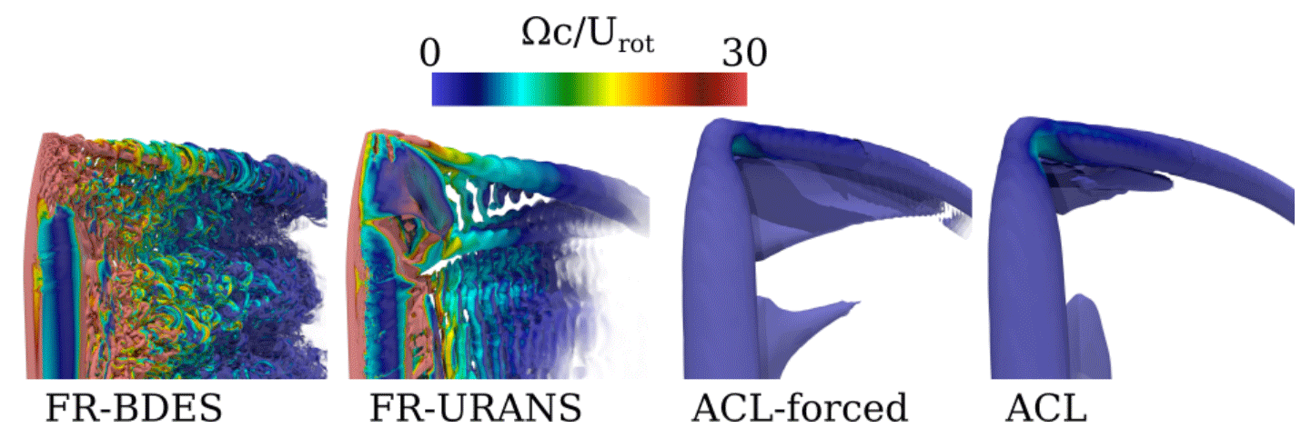
Figure 5 Comparison of the early tip vortex formation between different turbulence and turbine simulation approaches.

5.1.3 The topology of the root vortex

The general structure of the root vortex is compared for the simulations in Fig. 6. The contour color is the helicity to investigate the sense of rotation of the vortices along the streamwise direction. In the FR-URANS simulation the root vortex consists of two vortex legs, which originate from the horseshoe vortex that lies in the junction of the blade connector and the nacelle. The helicity shows that at the horseshoe vortex the two legs are counter-rotating. Farther downstream, they roll up into a single vortex that rotates in the sense that there is a flow around the blade root from the pressure to the suction side. The vortex braid itself spirals around the nacelle in the opposite sense of its self-rotation. The mutual interaction of the still-separated vortex legs leads to the formation of secondary vortices. These arise because the main vertebrae are being stretched. Opposed to the URANS simulation, the FR-BDES can resolve the detailed flow phenomena going along with the massive flow separation in the inner blade region. Two flow topologies can be observed, which are depicted in the upper-right sub-figures, namely a trailing and a shedding topology. It is typical of vortex shedding phenomena that their intensity modulates in time (Mockett, 2009). During weak shedding events, a trailing topology like that of the URANS solution is formed, although it is highly superimposed by smaller-scale turbulent eddies. During strong shedding events, the lower leg is destroyed, and the detached flow is deflected in the outer direction into which the roll-up of the root vortex is also directed. The roll-up itself is then also less coherent than in the case of weak shedding. In the ACL method where the forces are injected from the FR-BDES, there is only one single vortex braid that spirals around the nacelle, as there is naturally no junction flow that could form a horseshoe vortex. Compared to the FR-URANS simulation, the ACL-forced simulation reveals smaller-scale turbulent structures. These vortices appear because the main root vortex is stretched by the boundary layer of the nacelle and also due to the velocity gradients caused by the rotor induction. The scale-resolving turbulence model facilitates the breakdown into smaller and smaller eddies. In the FR-URANS simulation, this evolution is limited to the largest scales. The standard ACL simulation involves a more complex vortex system in the root region, which is illustrated by means of a view upstream and downstream of the actuator line. In the inner rotor region, a second bound vortex prevails that is enclosed by two trailing legs. The outer one rotates in a counterclockwise direction with respect to the flow vector, whereas at the inner end, a counter-rotating vortex pair is formed. This vortex pair is deflected outwards. Inwards of it, the actual root vortex develops. Due to the outward deflection of the whole vortex system, it is lifted from the nacelle surface at the beginning.

Figure 6 Comparison of the root vortex formation between fully resolved URANS and BDES simulations with the two actuator line simulations.

These observations can be explained in more detail when relating them to the blade loading and particularly the distribution of the circulation. Both are discussed in the next section.

5.2 Blade loads, circulation and trailed vorticity

The time-averaged sectional blade loads are presented in Fig. 7. They are based on pressure integration in the normal and tangential direction of the local blade chord and exclude the friction forces. Note that the later used tangential velocity in the wake is defined tangentially to the rotor plane with a positive sign in the sense of blade rotation. In the experiments, the forces are integrated from the pressure taps with the trapezoidal rule. Due to the sparse distribution of sensors in the aft-chord region, the trailing edge point is approximated consistently to Parra (2016) by taking the average of the last available sensors in the chord direction from the pressure and suction side. In the simulations, two different evaluation methods are compared: the first calculates the forces by integration of pressure over the entire surface. The second utilizes only the data points at the location of the pressure taps in the experiment. In the actuator line method, the forces stem directly from the respective actuation nodes, where the BEM is evaluated.

Figure 7 Sectional normal (a) and tangential loads (b). Comparison of simulations with experiments. The lines show the forces determined from pressure integration of the entire surfaces. The symbols are based on pressure integration at the positions of the sensors as in the experiment.

In general, it becomes apparent that the simulations tend to overestimate the normal and tangential loads, particularly in the outer blade region. However, it must also be noted that the deviations in the inner and middle part of the rotor are at least partly a matter of the post-processing. It can be shown that by evaluating the loads solely based on the positions of the pressure taps, an overall improvement in the agreement is achieved, yielding an almost-perfect match for the two inner sections. At $\frac{r}{R}=\mathrm{0.6}$, the overestimation of the normal loads might be due to the fact that the actual geometry, and thus blockage effect of the zig-zag tape, is not considered in the simulations. It was suspected within the Mexnext III project that the latter may cause an overtripping in the experiment, particularly in the Risø section, and consequently leads to a larger extent of the flow separation. In the region of the blending between the Risø and the NACA 64 airfoil, the URANS and the BDES simulations show a very similar behavior in the mean loads, namely strong spanwise gradients. These are linked with gradients in bound circulation, which are detailed in Fig. 10. They are in equilibrium with the two trailed vortices being created in the transition zones between the airfoils. Such strong gradients in the loads were not visible in any previous simulations on this operating point but might eventually be captured by the substantially finer grids employed within the present study. As there are no experimental data in this region, a comprehensive validation is not possible. At the two outer sections, the overestimation of the normal loads is associated with the problem of a too-small tendency of flow separation, which is a typical tendency of the employed k–ω SST turbulence (background) model (Matyushenko and Garbaruk, 2016). The FR-BDES nevertheless shows an improvement compared to the URANS approach. The advantage of the BDES is especially pronounced in the tangential forces, which are significantly influenced by the pressure drag of the separated flow at each profile cut. This suggests that generally the extent of the flow separation seems reasonably predicted. Only again in the outer sections is there a slight overprediction of the tangential forces corresponding to the separation area predicted there being too small.

The difference in the wake topology between the ACL with standard two-dimensional polars and with the forces from the fully resolved simulation can be explained by looking at the differences in the loads. Being calculated based on the polars, the normal and tangential loads are significantly lower than in the fully resolved counterparts, particularly in the inner rotor region. Very similar force distributions were obtained by all partners in the validation rounds working with lifting-line methods and did not employ a rotational augmentation model, while other BEM codes with respective models showed higher loads and better agreement with the measurements (Boorsma et al., 2018). In the transition zones between the airfoils, the force gradients are much smaller. First, there are no measured polars in the transition zones. Therefore, the BEM interpolates them from the adjacent airfoils, i.e., between the DU91 and the Risø for the inner transition zone and between the Risø and the NACA64 for the outer zone. Comparing the measured polars (see Fig. 8), it can be seen that the stall onset of the airfoils is different. The Risø airfoil has a higher C_L,max and a harder stall compared to the DU91 airfoil and the NACA64 airfoil. However, looking at the angles of attack at which the turbine operates (see Fig. 10), it can be seen that in the $\mathrm{0.45}\le r/R\le \mathrm{0.75}$ region the angles are between 20 and 13°. This means that for the ACL with two-dimensional BEM calculation, all polars are effectively in the post-stall regime where very similar lift values are obtained. Thus, the spanwise gradients between the individual airfoils in the transition zones become small. On the other hand, in the blade-resolved simulations, three-dimensional effects such as crossflow cause the airfoils not to operate in the flat post-stall regime, and the different behavior of the airfoils in the stall region comes into play more than in the ACL with BEM forces. In the outer blade region where $\frac{r}{R}>\mathrm{0.75}$, a comparable agreement to the fully resolved simulations is achieved.

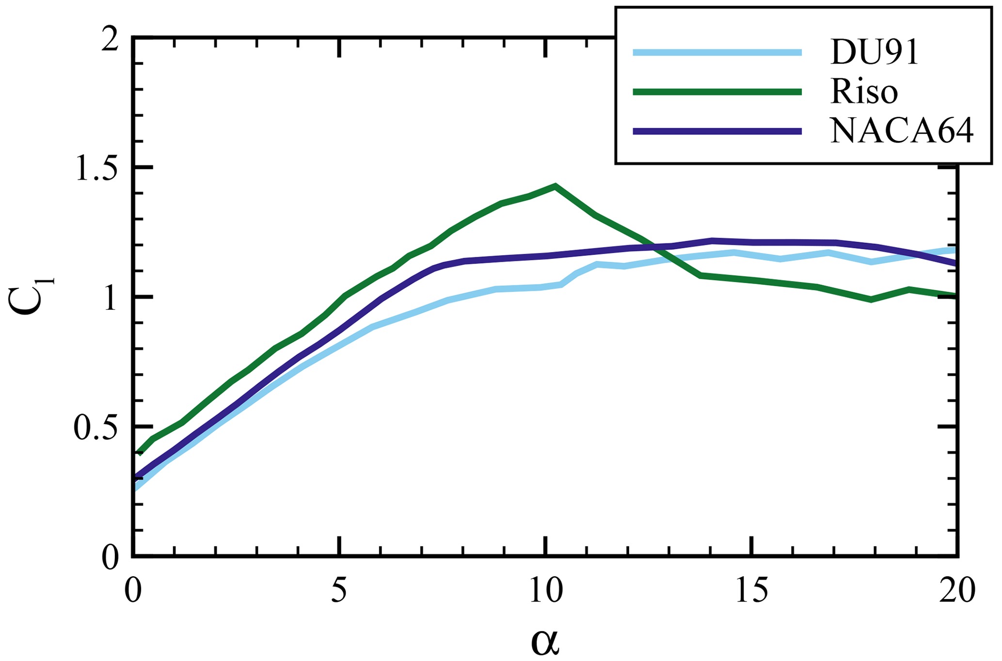
Figure 8 Measured two-dimensional lift polars of the DU91-W2-250, the Risø-1-21 and NACA64-418 airfoils (reproduced from Schepers et al., 2012).

An evaluation of the bound circulation is shown in Fig. 10. It aims to better understand the formation of trailing vortices and, more importantly, to supply evidence on objective 3 stated in the outline, namely, to clarify whether the same wake of a fully resolved simulation is obtained when imposing their forces onto the ACL. For this purpose, the circulation distributions evaluated in the flow field of both simulations are compared. If they do agree well, it can be expected that very similar mean velocities are also obtained in the wake. Moreover, the validity of the Kutta–Joukowski theorem can easily be verified by comparing lift, recalculated using the evaluated bound circulation in the ACL forced with lift from the surface loads of the FR-BDES simulation.

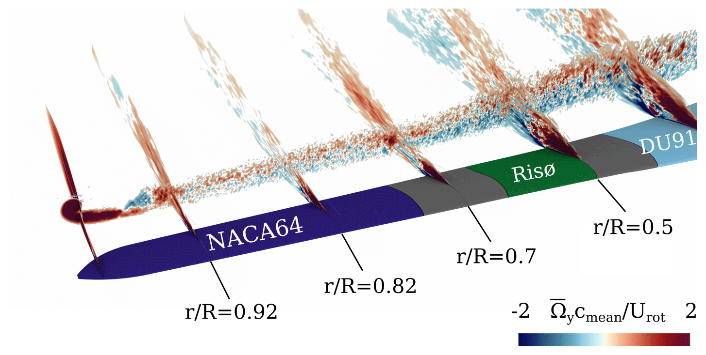
Figure 9 Time-averaged chordwise vorticity in the separated wake, indicating trailing vortices in the transition regions between the airfoils. Simulation FR-BDES.

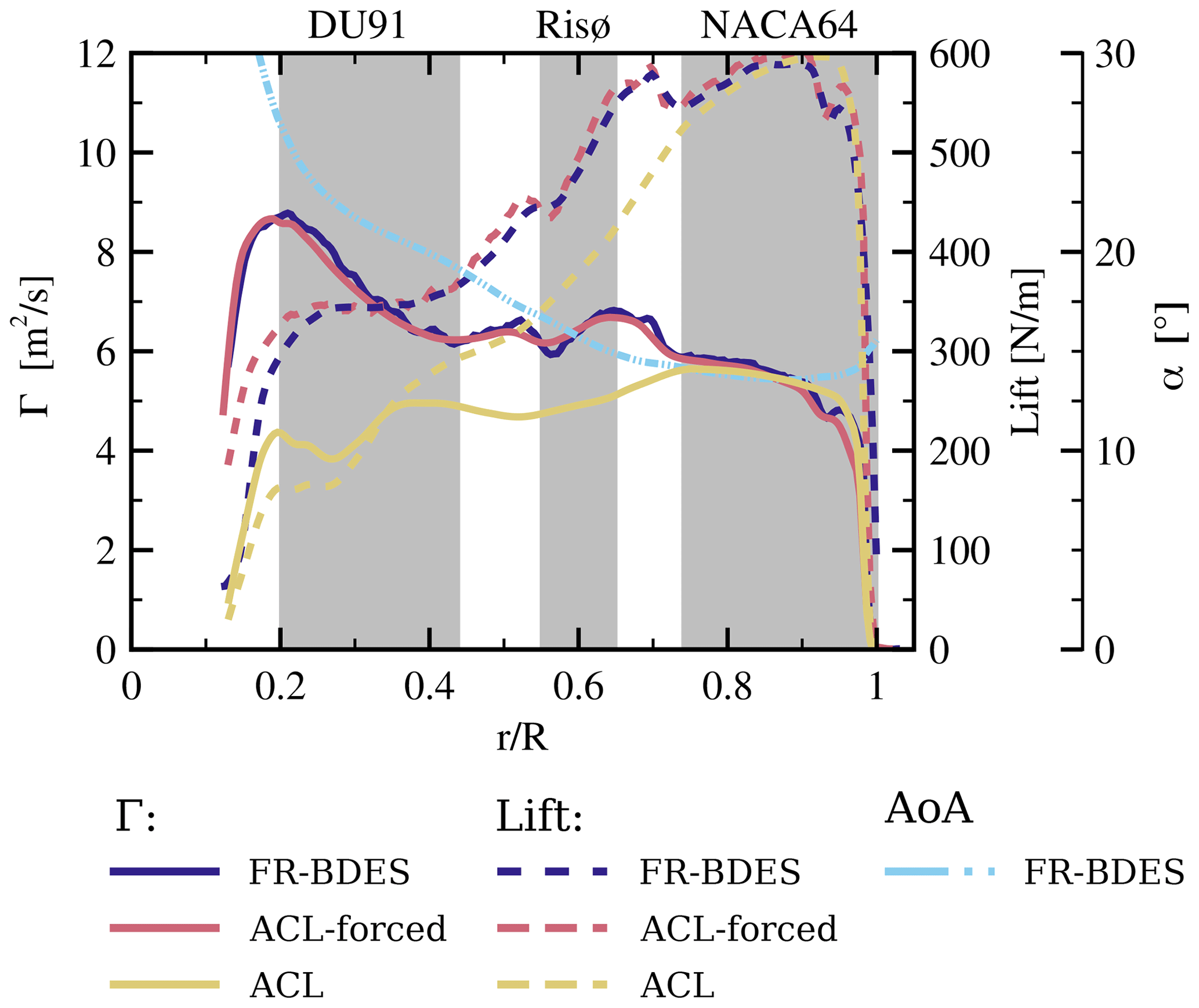
Figure 10 Radial distributions of the bound circulation Γ and the sectional lift forces. The latter as calculated with the Kutta–Joukowski theorem, the surface loads from FR-BDES and the extracted angle of attack. The grey patches indicate the locations of the different airfoil types.

In the graph, circulation is displayed as solid lines and lift as dashed lines. The FR-BDES, the forced ACL and the standard ACL method are given in blue, rose and sand colors, respectively. The circulation was determined from the time-averaged velocity fields extracted on a cylindrical surface with 0.37 m radius around the blade by integrating along closed circular curves in each section of the hull using the relation $\mathrm{\Gamma }=\oint \mathit{u}\cdot \mathrm{d}\mathit{s}$.

Firstly, it can be observed that the fully resolved simulation agrees very well with the forced ACL. This also holds for the comparison of lift, where the recalculated one from the Kutta–Joukowski theorem almost perfectly matches the distribution evaluated from the surface of the FR-BDES simulation, besides some minor deviations in the very inboard region. The required angle of attack was evaluated using the method of Jost et al. (2018), by averaging the axial and tangential velocities on the hull surface in the same way as calculating the circulation. This gives a clear indication that imposing forces stemming from fully resolved simulations directly into the actuator line result in the same circulation, even in separated flow, and, consequently, it can be expected that a very similar induction and mean velocity distribution are also obtained in the near field of the blade.

When comparing the standard ACL model to the above, a significantly smaller circulation is generated, particularly in the inner blade region. This already implies a much lower induction of the rotor in that area and emphasizes the necessity of considering corrections for rotational effects in BEM or lifting-line codes when flow separation is encountered in the root region of the blade.

As the gradients in the circulation behave proportional to the trailed vorticity, they are looked at more closely to explain the observed trailing vortices in the flow visualizations. In the FR-BDES it is difficult to identify these vortices in the instantaneous iso-surfaces of λ₂, as they are heavily overloaded by small-scale turbulence. Therefore it is referred to in Fig. 9, where the temporal mean of the vorticity component in the chordwise direction is depicted.

The overall largest gradients appear at the root and the tip, in all simulations, and are in equilibrium with the root and tip vortices, respectively. However, as already suspected from the loads, significant local gradients appear in the transition zones to and from the Risø airfoil but only in the FR-BDES and the ACL-forced simulation. These gradients correspond to the trailing vortices in the middle part of the blade, which are not present in the standard ACL, as observed in Fig. 4. Moreover, close to the tip at $\frac{r}{R}\approx \mathrm{0.95}$, the distribution shows a small dip which is slightly more pronounced in the FR-BDES than in the ACL-forced simulation. It is represented by an additional trailing vortex inboard of the main tip vortex. This dip in the circulation is not present in the standard ACL. Thus, also no additional vortex evolves at the respective position. On the other hand, this simulation features a spot of a negative and then positive gradient in the inner region $\frac{r}{R}\approx \mathrm{0.2}-\mathrm{0.35}$ not appearing in the other simulations. This explains the additional trailing vortices observed in Fig. 6. The root vortex and the outer trailing leg of the vortex system that both exposed a negative helicity are associated with the positive circulation gradient. On the other hand, the vortex slightly outboard of the actual root vortex that revealed a positive helicity corresponds to the negative circulation gradient.

5.3 The wake of the blade

The wake of the blade mainly reflects the induction effects caused by the aerodynamic forces discussed before. However, viscous effects stemming from the boundary layers or, on a larger scale, separated shear layers are also visible in the blade wake. With the actuator line simulations, imprints of the bound vortex also result in shear layers that create a similar pattern in the flow field to the viscous and separated shear layers, although they originate from the integral aerodynamic forces of the blade section.

5.3.1 Comparison of flow structures with PIV

In order to assess the flow structures in the close vicinity of the blade, its passage through the horizontal PIV plane is traced. Therefore, the instantaneous axial, tangential and radial velocity components are evaluated in Figs. 11–13. They are displayed for three different phase angles relative to the PIV plane, namely at $\mathrm{\Delta }\mathit{\theta }=\mathrm{13},\mathrm{20}$ and 40°. The measurements were gathered on four PIV sheets, which cover the area spanning from 0.065 m (0.029 R) to 0.436 m (0.194 R) in the streamwise direction and from 0.367 m (0.147 R) to 2.683 m (1.073 R) in the radial direction. The borders of the PIV sheets are included in the simulations to support the comparison. Additionally, a line marking the location of the radial velocity traverses is included. These results are discussed in Sect. 5.3.2.

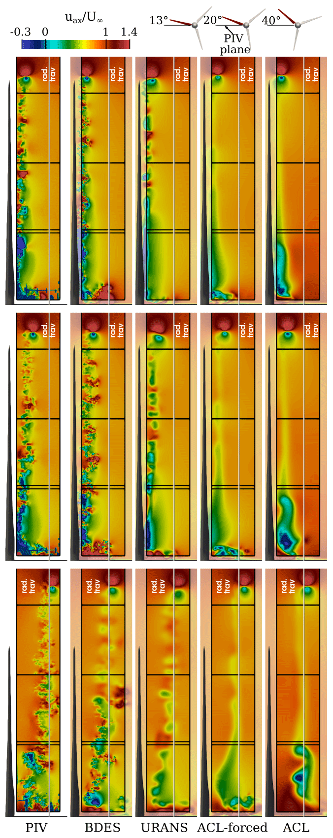
Figure 11 Evolution of the instantaneous axial velocity in the blade wake in planes 13, 20 and 40° (from top to bottom) downstream of the blade. Experimental results are from Boorsma and Schepers (2015).

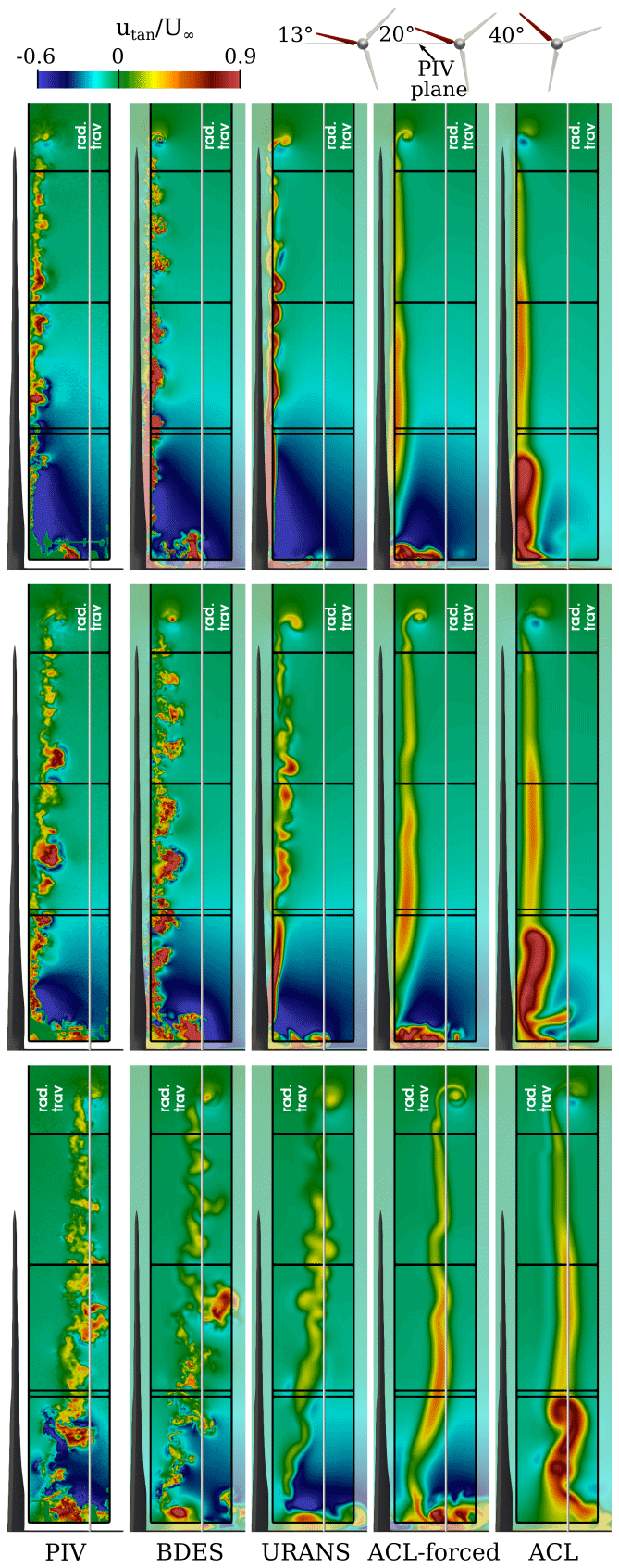
Figure 12 Evolution of the instantaneous tangential velocity in the blade wake in planes 13, 20 and 40° (from top to bottom) downstream of the blade. Experimental results are from Boorsma and Schepers (2015).

Figure 13 Evolution of the instantaneous radial velocity in the blade wake in planes 13, 20 and 40° (from top to bottom) downstream of the blade. Experimental results are from Boorsma and Schepers (2015).

At the phase angle Δθ=13°, where the separated flow field has just entered the evaluation plane, the experiments show alternating cells of high and low axial velocity along the middle and outer blade regions. The bubble-shaped areas of high tangential velocity emphasize the alternating sizes of the separation area and indicate the presence of stall cells. In the inner region, where the blade is just entering the plane, the axial velocity is negative, as a consequence of the downwash of the blade and the generation of lift. This goes hand in hand with a negative tangential velocity due to the large circulation and results in a deflection of the streamlines into the plane. Directly at the root, the spot of positive velocity indicates the formation of the root vortex that pushes the flow on the suction side radially outward (see radial velocity in Fig. 13). At the blade tip, the corresponding tip vortex has already formed since the evaluation plane is situated some chord lengths downstream of the blade. The circumferential velocity around the vortex axis is reflected in the axial and radial velocity (related to the rotor). The axial velocity of the tip vortex is aligned approximately with the tangential direction of the rotor. However, the tilting of the vortex helix with respect to the evaluation plane, which is not negligible due to the small tip-speed ratio of the rotor, leads to a spot of positive tangential velocity at the upper border of the vortex and a negative spot on the bottom side.

Comparing the simulations with the PIV measurements in the first plane, it can be found that the FR-BDES simulation yields a structurally very similar flow pattern, namely alternating patches of axial velocity in the middle and outer parts of the blade. These patches show up as bulbs carrying positive tangential velocity and emphasize the modulation of the separated flow of the blade. Compared to the experiment, the predicted magnitude of the velocity is slightly higher in the mid-blade region, while quantitatively similar levels are obtained in the outer sections. The sizes of the turbulent eddies are even finer in the FR-BDES than in the PIV. This is because of a higher spatial resolution in the near field of the blade in the simulations, which is 1.4 mm for the inner half of the rotor and 0.7 mm in the outer portion, compared to a maximum PIV resolution given as 2.14 mm (Boorsma and Schepers, 2015). Compared to that, the velocity field in the FR-URANS simulation is less fine-grained, although the main alternating vortex structures in the middle and outer blade regions are also present as they can be retrieved especially from the axial velocity field. In the ACL simulations, by definition no viscous blade aerodynamics can be taken into account. Therefore, the detailed and transient separation features and their imprint into the very near wake of the blade cannot be resolved. Indeed, for a fairer comparison of ACL, the time-averaged fields from PIV and the full-resolution simulations would need to be used. The very basic flow patterns that mainly depend on the integral airfoil forces are nevertheless captured, as can be seen in the qualitatively similar shape of the tangential velocity. Here, the standard ACL shows a more homogeneous flow field in the middle and outer blade regions compared to the forced ACL. This is aligned with the fact that the forces and their gradients are much smoother in the standard ACL compared to the forced variant, which is in accordance with the previously made observations on the generation of the trailing vortices.

In the inner blade region, the flow field is very well predicted by the FR-BDES simulation. This applies to the deceleration of the flow in the axial direction, its strong deflection in the negative tangential direction and its redirection in the positive radial direction. The first two effects are due to the strong circulation of the blade in the inner portion, whereas the region of positive radial velocity represents the suction side part of the root vortex that is building up. The spot of positive tangential velocity near the vertical line that marks the extraction of the radial traverse shows the tail of a preceding shedding event as described in the flow visualization of Fig. 6. Apart from the absence of small-scale turbulence, the FR-URANS simulation provides a very similar picture compared to the BDES simulation; i.e., the range of influence of the root vortex in all velocity components is narrower than in the FR-BDES and the experiments. Accordingly, there is no vortex shedding in the inner blade area. The ACL-forced simulation shows a similar pattern in the root vortex region for the tangential and radial components to the FR-BDES simulation, from which it inherited the forces. Overall, however, the flow deflection in the tangential direction appears to be less pronounced than in the fully resolved simulations and the experiment. Relative to this, however, the deviations of the ACL, in which the forces are calculated internally by the BEM, are significantly larger. The deceleration in the axial direction is smaller, and the deflection of the flow in the negative tangential direction in particular is completely absent. Instead, the secondary vortex system shown in Fig. 6 begins to form. This flow pattern correlates in detail with the clearly underestimated blade loads in the normal and tangential directions compared to the experiment, as well as the associated distinctly reduced circulation in the inner blade area discussed in Fig. 10.

In the tip region, the roll-up process of the vortex occurs similarly in all simulations. The best agreement with the experiment is obtained with the FR-BDES simulation. In the FR-URANS simulation, the tip vortex is already deformed and more oval than in the experiment. The ACL simulations predict the shape correctly, although the initial strength seen in the peak velocities slightly differs between forced and standard ACL. There are differences in the tangential velocity pattern of the tip vortex. In the FR-BDES, the shape is very similar to the experiment, however, with slightly stronger peak values in both directions. The positive spot in the upper border of the tip seems to be highly pronounced and is even more pronounced in the FR-URANS and in the forced ACL compared to the FR-BDES simulation. On the other hand, the negative velocity spot at the lower end of the tip vortex is overly pronounced in the standard ACL. Especially when tracking the evolution in the planes further downstream, the strength of the tangential velocity in the tip vortex seems to depend on the strength of the shear layer being rolled up. In the forced ACL, this layer of positive tangential velocity remains coherent. The roll-up of the tip vortex stretches the shear layer and thereby transports high values into a concentrated spiral around the main tip vortex (significantly stronger than in the experiment). In the ACL with internal force calculation, this layer is more blurred. The reason might lie in the bi-directional coupling of the forces and the wake flow. Hence, variations in the flow field will vice versa cause variations in the forces and lead to an overall thicker and less concentrated shear layer. Of course, this mechanism does not exist in the variant with constantly applied forces. By comparison, the shear layer in the fully resolved simulations includes the viscous effects of the separated blade wake. Thus, especially with the scale-resolving turbulence modeling, the shear layer mixes and becomes less coherent than in the ACL-forced simulation. Consequently, a less pronounced and less concentrated spiral of positive tangential velocity is also rolled-up around the tip vortex. This is also in overall good agreement with the PIV measurements. In the FR-URANS simulation, however, a higher blurring is visible due to the dissipating nature of the underlying turbulence modeling.

When looking at the propagation of the separated wake in the middle and outer parts of the blade (note that the PIV results are not temporally correlated to the planes before), the turbulence pattern is again very similarly predicted in size and shape by the FR-BDES. The mushroom-like structures have become larger during the development from the previous slice. At the position Δ=40° relative to the blade, a large-scale turbulence bale has developed in the wake of the mid-blade region, a narrow turbulence band in the inboard area and a relatively homogeneous wake in the outer part of the rotor. Regarding the resolution of small-scale structures, good visual agreement is found only in the inner half of the rotor. Farther outboard, however, where the distance of the slice to the blade has increased, the wake is already in the coarser grid level, and, therefore, the eddies become blurred. In the FR-URANS simulation, the changes along the different evaluation steps are primarily related to inviscid induction effects that govern the motion and interaction of the largest modes being resolved. Any other turbulence-related cascade of vortex breakdown is diffused by the turbulence model. This is the typical and expected behavior of the URANS approach and is commonly referred to as the “spectral gap”. Likewise, the ACL flow field is also primarily driven by inviscid effects (except for the wall-bounded part near the root). However, in comparison to the URANS simulation, the diffusion is minimized by using a scale-resolving turbulence model. Since there are no external perturbations, like gusts or inflow turbulence, the wake remains rather stable in the near field of the blade. First, deformations are nonetheless initiated with the ACL-forced simulation at Δ=40° due to the high gradients in the bound circulation of the ACL-forced simulation that initiate a deformation wake.

Turning finally to the propagation of the flow in the root region, the details of the described flow topology in Fig. 6 can also be found in the PIV snapshot with a phase angle Δ=40° to the blade. The plane is located temporally in between two strong shedding events and thus captures a trailing event in which the root vortex is rolled up. This can be retrieved from the areas of alternating sign in the axial and radial velocity components. Unlike the tip vortex, which is almost circular, the root vortex becomes elliptical by the presence of the shear in the boundary layer of the nacelle. An important detail to be noted is the small patch of positive tangential velocity at the edge of the PIV plane observed in both the FR-BDES simulation and the experiment. A close examination of the λ₂ isosurface in Fig. 6 has shown that the evaluation plane intersects the offshoots of the previous shedding event. The fact that this spot is very similarly found in the experiments gives a clear indication of the actual occurrence of the described alternations of the root vortex topology. In the FR-URANS and ACL-forced simulations, the root vortices develop quite similarly to each other. However, as already noted for the first evaluation level, it is somewhat flatter in the FR-URANS simulation. Lastly, the most significant deviations occur in the standard ACL simulation. In particular from the radial velocity component, it can clearly be seen how the two additional inboard vortices previously described in Fig. 6 are developing. These vortices also inhibit the classical velocity pattern expected of the root vortex.

5.3.2 Radial traverses

The radial traverses of the velocities were extracted at the streamwise constant lines previously shown in Figs. 11–13. Nominally and according to the experimental data reduction document (Boorsma and Schepers, 2015), the traverses should have been extracted at x=0.3 m (0.13 R) downstream of the rotor. However, Schulz et al. (2016) found a misalignment of the coordinate systems by around ∝0.045 m. For this reason, the extraction line was corrected to the position x=0.345 m (0.153 R) for both experiments and simulations. The cross-plotting of the PIV data and the different simulation approaches are shown in Fig. 14. Again the phase angles relative to the blade of $\mathrm{\Delta }\mathit{\theta }=\mathrm{20},\mathrm{40},\mathrm{60}$° are evaluated. Additionally, an azimuthal average over the 120° period is presented in the top row of the figure. This averaged traverse was the main benchmark in the Mexnext III project. It is calculated by a weighted sum of all the recorded traverses (not only 20, 40 and 60°) with a weighting factor representing the phase increment between the individual traverses. In contrast to the previous evaluations, which compared the flow structures based on the instantaneous fields, the phase-averaged velocity is considered here. In the experiments, this was achieved by ensemble averaging the 31 temporally uncorrelated PIV images. In the simulations, the time averaging was carried out in the moving reference frame over 1 revolution. The data were then extracted under the respective phase angle relative to the blade. In the measurements, the error bars shown as the grey background denote the standard deviation of the velocity. Note that for the azimuthal average, the weighting is applied equally to the standard deviation.

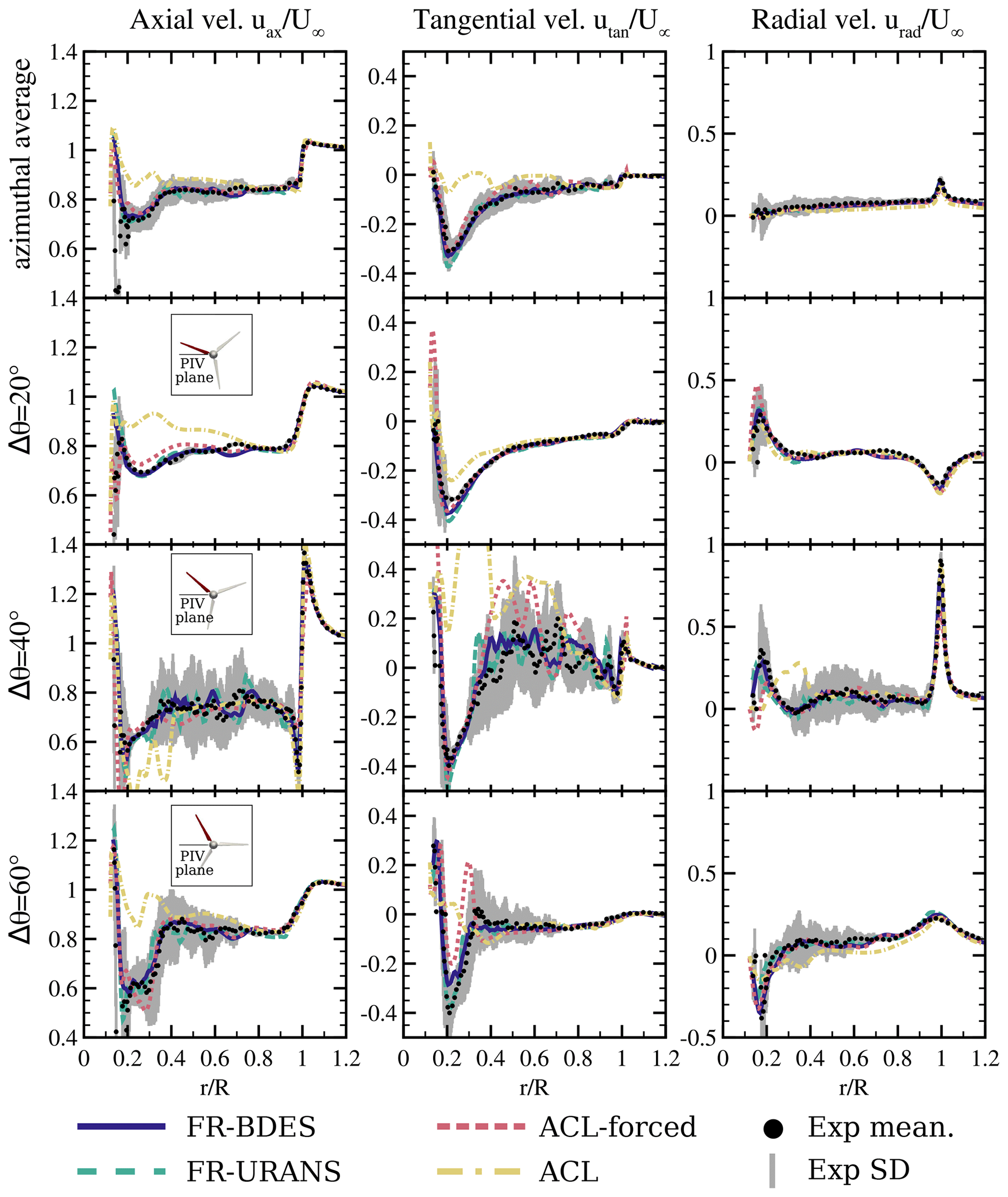
Figure 14 Radial traverses of the axial, tangential and radial velocities, evaluated $\frac{r}{R}=\mathrm{0.153}$ downstream of the rotor plane at different azimuthal positions relative to the blade (Δθ) as well as azimuthally averaged. All results are phase averaged. Comparison of different simulation approaches with the PIV experiment of Boorsma and Schepers (2015).

The azimuthal average of the axial velocity is shown in the upper-left graph of Fig. 14. Overall, good agreement of simulations and measurements can be observed. The only significant deviations appear with the ACL simulation in the inner region, where induction is generally too small. In the outer part, all simulations agree well with the measurements. It is worth noting that the previously observed overestimation of the loads in the outer rotor area is hardly discernible in the velocity deficit. The drop in the inboard region between $\frac{r}{R}=\mathrm{0.2}$–0.4 is seen to be caused by the large normal-force coefficients in this area. Note that for the design case at tip-speed ratio Λ=6.7, this dip did not occur, and also the blade-normal loads did not show a relative increase in that section. This effect is clearly associated with the rotational augmentation of lift in the inboard region of the blade. In the ACL simulation based on the uncorrected two-dimensional polars, this effect is not included. Likewise, the underprediction of the normal loads and the associated reduced circulation in that region lead to a significant underprediction of the axial induction in that region. In the ACL with imposed forces, the agreement is very good for the azimuthally averaged wake. Only in the early stages of building up the wake (cf. Δθ=20°) is the flow less retarded than in the experiment. At the plane Δθ=40°, the separated flow and also the tip vortex reach the evaluation traverse. Excellent agreement is achieved for all simulations. However, it must be noted that the correction of the evaluation position in the experiments is crucial to correctly capture the large gradients around the tip vortices. The separated flow, which stems from the middle and outer blade regions, yields expectedly strong fluctuations. In the inner portion, the fluctuations are lower since this part of the separation area travels slower. All simulations closely match the measured velocities of the PIV. Only in the inner part does the secondary vortex system evolving in the standard ACL lead to a downward excursion in the velocity. At Δθ=60°, the separated area of the root region has arrived, imposing large fluctuations, whereas the fluctuations in the outer area have diminished. Again, very good agreement is obtained for all simulations, except for the case of the standard ACL in the inner part of the blade.

Turning to the tangential component u_tan, its profile is similar for all evaluated azimuth positions, showing a distinct minimum at around $\frac{r}{R}=\mathrm{0.2}$ followed by a rise towards the tip. Generally, the values are supposed to be negative as the wake rotates in the opposite direction of the rotor. The only exception, where positive values are obtained, is when the separated wake flow of the blade reaches the evaluation line (see Δθ=40°). Due to the principle of “action and reaction”, the rotor can only be driven if it sets the wake into counter-rotation; it is intuitively clear that the positive tangential component caused by the flow separation reduces the turbine power. The strong dip in the inner blade region, which is visible as the dark-blue contour in Fig. 12, is again the consequence of the high bound circulation in the root region boosted by the effect of rotational augmentation. Indeed, pressure coefficients of up to $C_{\mathrm{p}}\approx -\mathrm{8}$ (see code comparison in Boorsma et al., 2018) were obtained on the suction side of the blade. In the standard ACL without respective correction for the rotation effects, the associated deflection of the flow is significantly less pronounced. All other simulations yield very accurate simulations in that region. At Δθ=40°, the ACL-forced simulation tends to predict a too-positive tangential velocity in the mid-blade region. This overprediction is even more pronounced in the standard ACL simulation. It implies that the shear layer in the ACL simulations stemming from the injection of body forces is somewhat too concentrated compared to that of the fully resolved simulations that account for the effect of turbulent mixing. The force injection could be further tuned by employing different strategies for mapping them into the flow field (Cormier et al., 2021; Churchfield et al., 2017). In the tip region, all simulations capture the change in the sign of the tangential velocity from negative to positive values in position and magnitude. This implies that the roll-up and tilting of the tip vortex relative to the evaluation plane are predicted correctly. At Δθ=60°, where the traverse cuts the root vortex, the FR-URANS simulation yields the best agreement, whereas its BDES counterpart slightly underestimates the dip. In the forced ACL, the change in sign is too concentrated and not predicted as in the measurements. As already seen from the distribution of the axial velocity, the flow deflection in the tangential direction in the rotor blade inner area is only insufficiently represented in the ACL with internal force calculation.

In contrast to the other components, for which the general distribution was the same across all azimuth positions, this is not the case with the radial component. At Δθ=20°, which is before the arrival of the separated flow, the root vortex induces an outward velocity and, correspondingly, the tip vortex a negative component. In between, an overall outward motion prevails. Opposed to the axial velocity, the ACL-forced simulation is in good agreement with the experiments. At Δθ=40°, the tip vortex has just passed the traverse, and the root vortex has not arrived yet; both vortices induce a positive radial velocity as also shown in the lower rows of Figs. 11–13. The simulations very accurately capture the distinct peak in the radial velocity. The excellent agreement also holds for the azimuth of 60°, except for a slight underprediction visible in the standard ACL. At this time, the root vortex has passed and induces an inward velocity component. In the tip region, the traverse departs the influence region of the tip vortex. Returning to the azimuth-averaged graph, it becomes clear that most of the local effects are averaged out. What remains is an overall outward flow, which is slightly lower with the standard ACL compared to the other simulations. This is associated with an overall smaller thrust coefficient of the rotor that also leads to a reduced deflection of the outer flow around the rotor wake.

5.3.3 Summary of the development of the blade wake

The following conclusions can be drawn from the velocity field in the very near wake of the blade:

1. The general trend in the velocity field is well predicted by all fully resolved and actuator line simulations.

2. The scale-resolved simulation on a highly resolved grid provides a very detailed view into the physics and the development of turbulent structures.

3. The URANS approach is sufficiently accurate in predicting the mean induction effects, even in separated flow.

4. The standard actuator line with internal force calculation and no model for rotational augmentation, as expected, underpredicts axial and tangential inductions in the inner part of the blade.

5. The falsely predicted forces and circulation gradients in the standard ACL induce a secondary vortex system in the root region, which has no physical basis.

5.4 The wake of the rotor

In the Mexnext projects, the wake of the rotor was characterized using axial velocity traverses. The corresponding evaluation plane is located 90° downstream of the rotor blade under consideration; i.e., the rotor blade is in a vertical position, while the data were extracted in the horizontal PIV plane. In the following, a qualitative comparison between the different simulations is again made using the instantaneous velocity contours before the axial traverses are compared as phase-averaged data. The velocity distributions of the PIV sheets are shown together with the predictions of the simulation in Fig. 15. The arrangement of the PIV sheets is marked again in the simulation graphs. The horizontal line labeled ax trav at $\frac{r}{R}=\mathrm{0.67}$ indicates the sampling locations of the phase-averaged data for the axial traverses, which are discussed in Sect. 5.4.2.

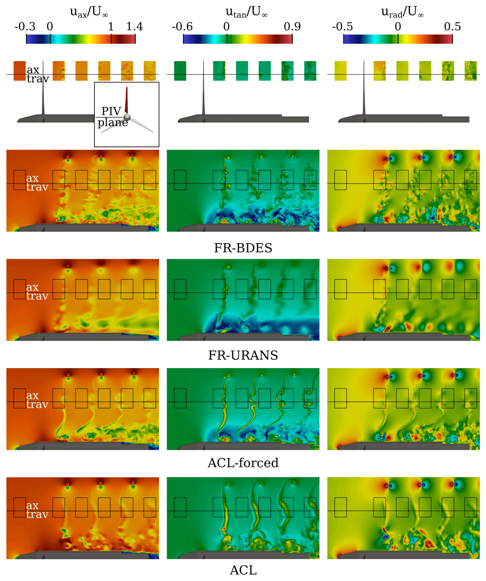
Figure 15 Comparison of the instantaneous flow field in the wake of the rotor in a plane located 90° downstream of the blade. PIV measurements are from Boorsma and Schepers (2015).

5.4.1 Flow structures in the rotor wake

In the FR-BDES simulation, the middle and outer areas of the wake show that the coherent structures disintegrate with increasing downstream distance. In particular, the velocity in the tangential direction shows that the wavy pattern, which was characteristic of the wake of the blade, breaks down towards homogeneous turbulence. This development is also confirmed by the experiments. However, due to the coarser computational grid in the wake compared to the PIV resolution, the simulated turbulence fields are more diffused. In the FR-URANS simulation, it can clearly be seen that any scale resolution is inhibited. The initially wavy shape in the tangential velocity is maintained. It appears to be only deformed by mutual induction effects. With increasing downstream distance these structures are increasingly diffused. Compared to the results of the fully resolved simulations, the ACL-forced simulation predicts significantly sharper velocity gradients in the middle and outer areas of the wake compared to the URANS flow field. This is firstly due to the turbulence modeling by using the same approach as the FR-BDES and secondly because of the stronger gradients in the shear layer generated by the body forces. With increasing downstream distance, it can be observed that the trailing vortices in the mid-region of the rotor start becoming unstable. Compared to that, the standard ACL reveals a less wavy pattern, which is also more diffusive than the pattern in the ACL-forced simulation. As already discussed before, the missing waviness is due to the absence of any trailing vortices in the mid-region of the rotor, and the increased diffusivity may be rooted in the bi-directional coupling of forces and the wake, which could have a damping effect on the imposed body forces.

Focusing on the inner region, the root vortex development can be traced by the alternating signs in the radial velocity component u_rad. In all simulations, except the standard ACL, they develop similarly. It can be deduced that its convection velocity is lower compared to the tip vortex due to overall smaller axial velocity in the inner region of the wake. Due to the shear, which is enhanced by the boundary layer around the nacelle, the root vortex starts mixing with the flow in the center. In the FR-BDES simulation, it also mixes with the resolved turbulence of the separated blade wakes. Along the axial direction, the thickness of the mixing layer increases. When reaching the position of the step in the nacelle geometry, no coherent vortex is visible anymore. In the FR-URANS simulation, the root vortex remains coherent without being mixed with the surrounding, but it is blurred out during the propagation. Opposed to this, the ACL-forced simulation predicts a very similar topology to its FR-BDES counterpart, also showing a disintegration towards small-scale turbulence. As there are no resolved eddies in the blade wakes, the mixing is slightly slower. In the standard ACL, the wrongly predicted development of the root vortex with its induced secondary trailing vortices together with the smaller induction in the inner part of the rotor also reduces the radial shear in the wake. Therefore, the mixing with the core flow is also less pronounced.

The latter observation on the actuator line method, namely that the wake remains more stable in undisturbed conditions but reaches a very similar topology to fully resolved simulations when it is disturbed, is a typical behavior already reported by Troldborg et al. (2015). In their study the disturbance was the turbulent inflow; here it is the shear of the flow in the root region.

5.4.2 Axial traverses

A quantitative comparison of the velocity fields is conducted based on the axial traverse crossing the mid-area of the wake at $\frac{r}{R}=\mathrm{0.67}$ (see Fig. 16). Phase-averaged results are plotted. The grey background shading indicates the standard deviation of the velocity fluctuations in the PIV measurements. The axial velocity implies the typical gradual deceleration of the flow when approaching the rotor, due to its blockage effect, and a further, more distinct retardation after passing the rotor plane being caused by its axial induction. The induction factor is only a_ax=0.13 at $\frac{r}{R}=\mathrm{0.8}$. This means that the average velocity is still about 75 % of the inflow velocity. In the simulations, the general shape of the blockage and the retardation of the flow in the wake are well predicted. Only the standard ACL underpredicts the blockage and the wake deficit due to the corresponding underprediction of the loads in the inner and middle portions of the blade.

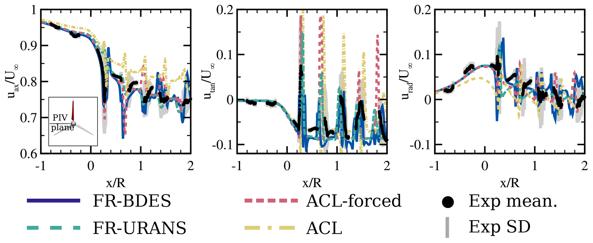
Figure 16 Axial traverse of the axial, tangential and radial velocity components, evaluated at $\frac{r}{R}=\mathrm{0.67}$. All results are phase averaged. Comparison of different simulation approaches with the PIV experiment of Boorsma and Schepers (2015).

Other than that, it can be observed that the axial velocity drops periodically when crossing the detached wakes of the blade. In the tangential velocity, this effect is even more pronounced as positive excursions. In both ACL simulations, these peaks are overpredicted, as the shear layers induced by the body forces are predicted to be too strong and too stable. This decay is more realistically captured by the fully resolved simulations. In the BDES simulation, the decay is a consequence of the resolved turbulent mixing, whereas in the URANS it is caused by the modeled turbulent viscosity. The general sense of the tangential velocity primarily indicates the rotation of the wake being opposed to the rotation of the rotor. It is interesting to note that the wake rotation already initiates slightly upstream of the rotor. In the wake it then remains effectively constant. All simulations slightly overpredict the magnitude of the wake rotation. This could be attributed to the overprediction of the loads in the tangential direction at that radial position. Turning finally to the radial velocity shown in the right panel of Fig. 16, it is characterized by a positive velocity upstream of the rotor as a consequence of its displacement effect. The nacelle possibly also contributes to this. This positive component decreases downstream of the wake as the expansion becomes asymptotic. All simulations but the standard ACL capture the general shape very well. In the latter a significant underprediction is visible already upstream of the rotor. The smaller induction results in a smaller blockage and thus a reduced deflection of the outer flow around the rotor. The spikes in the distribution stem again from crossing the vortex sheet of the viscous wake. Based on the circulation distribution, a positive amplitude can be expected from the former pressure side and a negative one from the suction side. Overall, these alternations are predicted by all simulations within the standard deviation of the experiments.

5.5 The tip vortices

The development of the tip vortices is mainly compared with the experiments of the first MEXICO campaign (Schepers and Snel, 2007). The reason for this is that only in the first campaign were the PIV planes placed such that they covered the tip vortex development. In the first MEXICO campaign, however, the entire span of the blade was equipped with boundary layer tripping. Therefore, it should be noted that there is a small inconsistency with the simulations, in which the outer flow section was treated as transitional. However, due to the high angles of attack, the effect of the transition on the loads in the outer blade region is minor. Hence, no major differences in the circulation and thus on the tip vortex development are expected. Unless otherwise described, the data were extracted in such a way that the rotor blade is located directly in the horizontal PIV plane during evaluation. The only exception is vortex 0 in Fig. 17, which was evaluated at a phase offset of 20° downstream of the blade and was obtained from the New MEXICO measurements. In all cases, the streamwise coordinate in the experiment was corrected by −0.045 m according to Schulz et al. (2016).

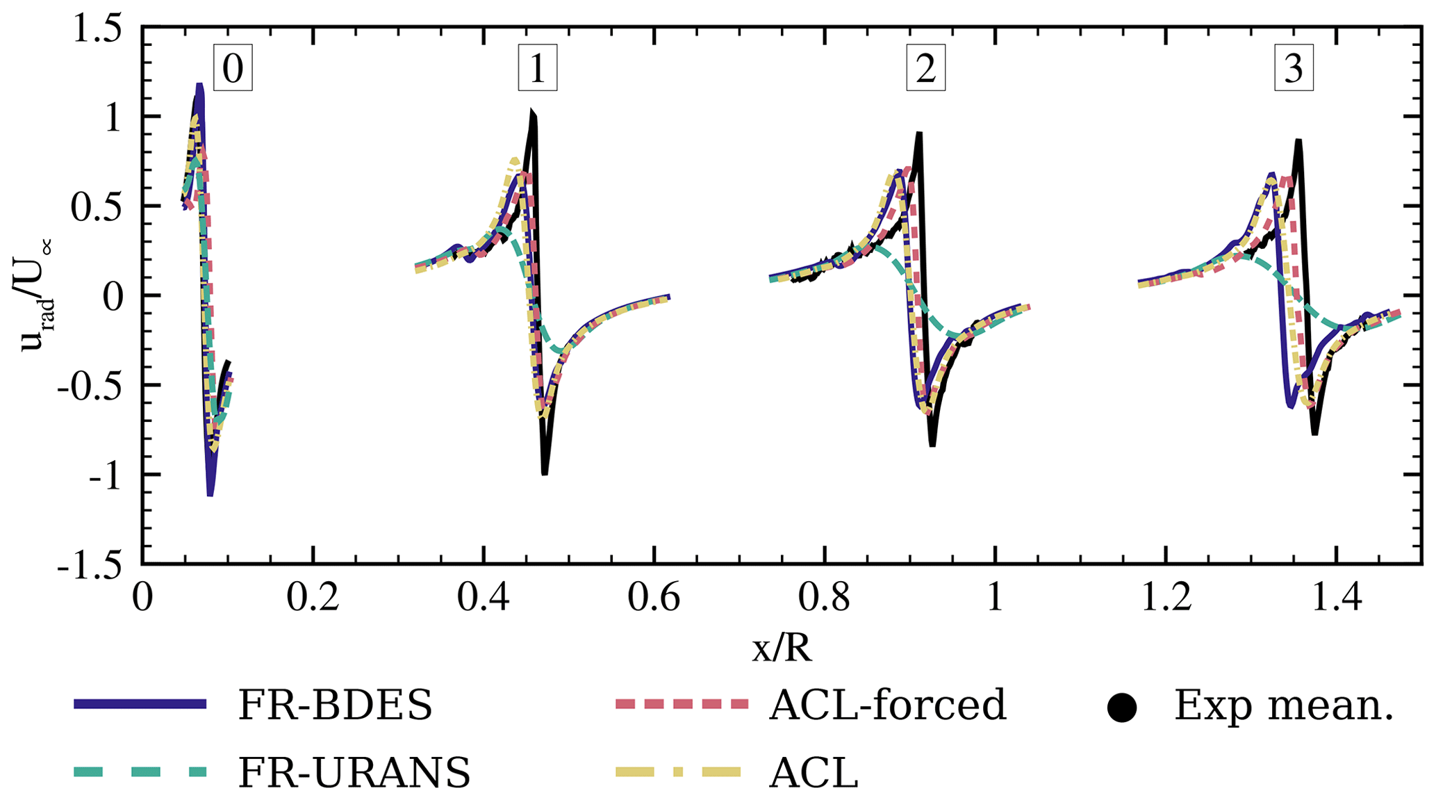
Figure 17 Comparison of the radial velocity in the tip vortex core. Instantaneous data. Comparison of different simulation approaches with the PIV experiment of Boorsma and Schepers (2015).

A first comparison of the vortex development is given based on the radial velocity (with respect to the rotor, which is the approximate circumferential direction of the tip vortex) traversing the vortex core in Fig. 17. The primary focus is on the amplitude of the velocity jumps rather than on the vortex-wandering dynamics. Therefore, the instantaneous field was evaluated, and the traverses were extracted for each case at the radial position, where the vorticity is maximum in the vortex core.

The streamwise position of the tip vortex agrees well for vortex 0 and vortex 1. Farther downstream, the FR-BDES simulation in particular lags behind the experiments slightly, suggesting a modestly slower propagation velocity. It should be noted that the vortex wandering will also influence the exact streamwise location of the vortex core. This effect was not corrected in the evaluation carried out here based on one snapshot and can lead to slight inaccuracies in the exact x position. However, since all simulations in all vortex cores have a bias to lower x coordinates, another cause for the systematic shift may be present, like for example a phase error between PIV and simulations or a slightly different axial induction or inflow velocity.

The velocity jump in vortex 0 is well captured by all simulations. Due to the higher grid resolution compared to the PIV sheet in that region, the gradient is even larger in the scale-resolved simulations than in the experiments. However, the FR-URANS simulation already shows a lower velocity jump. All simulations underpredict the amplitude of the experiments for vortex 1. Here, the grid spacing is around 6.6 % of the tip chord (stays constant up to vortex 3) and obviously too coarse to accurately capture the very sharp gradients in the vicinity of the vortex center. While the FR-BDES and the ACL-type simulations yield very similar maxima (with relatively higher values in the ACL-forced simulation), the FR-URANS simulation dramatically blurs the velocity across the vortex. This could already be expected from the previous examinations on the velocity field of the blade and rotor wakes. This trend also prevails for vortex 2 and vortex 3. It is interesting to note that the relative difference between all simulations (except the FR-URANS) and the experiment decreases slightly. By looking at the decay rates of the velocity jumps in more detail (summarized in Table 3), some insight can be gained into whether it is the physical aging of the vortex or numerical dissipation that changes the amplitude. The decay rates of the semi-empirical model of van der Wall et al. (2016) are used for comparison as a further reference. In this model the aging of the vortex core with respect to the azimuth angle ψ behind the blade is defined as

$$\begin{array}{}\text{(1)}& r_{\mathrm{core}}=r_{\mathrm{core},\mathrm{0}}\sqrt{\mathrm{1}+{\displaystyle \frac{\mathrm{5}\times {\mathrm{10}}^{-\mathrm{6}}}{{\left(\frac{r_{\mathrm{core},\mathrm{0}}}{R}\right)}^{\mathrm{2}}\mathrm{\Omega }}}\mathit{\psi }},\end{array}$$

where r_core,0 is the initial vortex core size assumed by van der Wall et al. (2016) as 5 % of the tip reference at 93 % rotor radius (=0.095 m), and Ω is the rotational speed of the rotor.

Table 3 Comparison of vortex aging between experiments, simulations and the semi-empirical model of van der Wall et al. (2016).

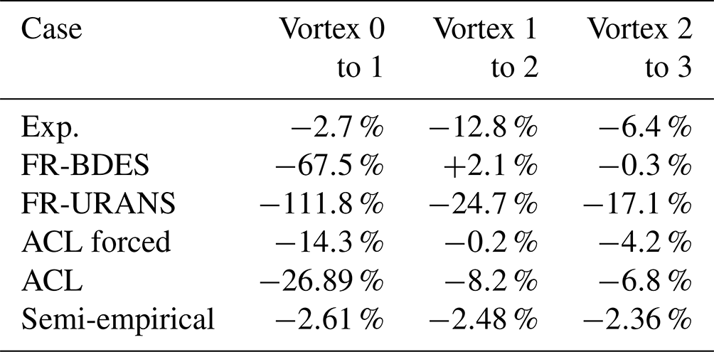
In the experiments, there is a very small reduction in the velocity jump (−2.7 %) from vortex 0 to vortex 1 followed by a larger reduction (−12.8 %) to vortex 2 and then again a smaller reduction (−6.4 %) to vortex 3. The small decay from vortex 0 to vortex 1 indicates that the PIV resolution is too coarse to fully resolve the vortex core. This has already been suggested by the PIV planes when we compared the blade wake in Sect. 5.3. Furthermore, it is also expected from the semi-empirical model that the decay rates are the largest at the early stages and then decrease with propagation time in a square root relation. The decay rates of the van der Wall model is overall smaller than in the experiment. In all simulations the significant decay from vortex 0 to vortex 1 is due to the increased grid spacing, in particular in the case of the FR-URANS, additionally due to the diffusion introduced by the turbulence model. In both ACL simulations the decay rate is lower than in the FR-BDES simulation since the initial vortex is larger due to the smearing of the actuation forces. From vortex 1 to vortex 2 and beyond, the decay rates of the FR-BDES and the ACL-forced simulation are lower than in the experiment. It seems that vortex growth is suppressed as long as numerical dissipation and diffusion through the turbulence model are small, and vortex resolution is limited only by a grid too coarse to fully resolve the physical size.

To obtain a quantitative measure for the quality of the different simulation methods, the vortex position, circulation, core radius and core vorticity are evaluated with the tip vortex analysis tool developed at IAG (Meister et al., 2011). This tecplot tool uses velocity slices as input and can easily be used with different sources of data, e.g., CFD, PIV or free vortex wake codes (Boorsma et al., 2018). The results are presented in Fig. 18. Two sets of measurement results are included. First, processing is based on the phase-averaged velocity field, which was the standard procedure in the Mexnext projects, and secondly, processing is based on an instantaneous flow field. The simulations are evaluated from instantaneous fields. Besides the simulations focused on in the present study, two further cases of the same authors are included, which were conducted during the Mexnext III project. These are IDDES simulations conducted on a full turbine model but on a wake grid approximately twice as coarse as in the present study. One simulation was performed with a standard second-order central difference scheme (JST) and one with a higher-order WENO scheme, as in the present study. The results from these simulations help us to understand the role of turbulence modeling, grid resolution and numerical schemes in the preservation of the tip vortices.

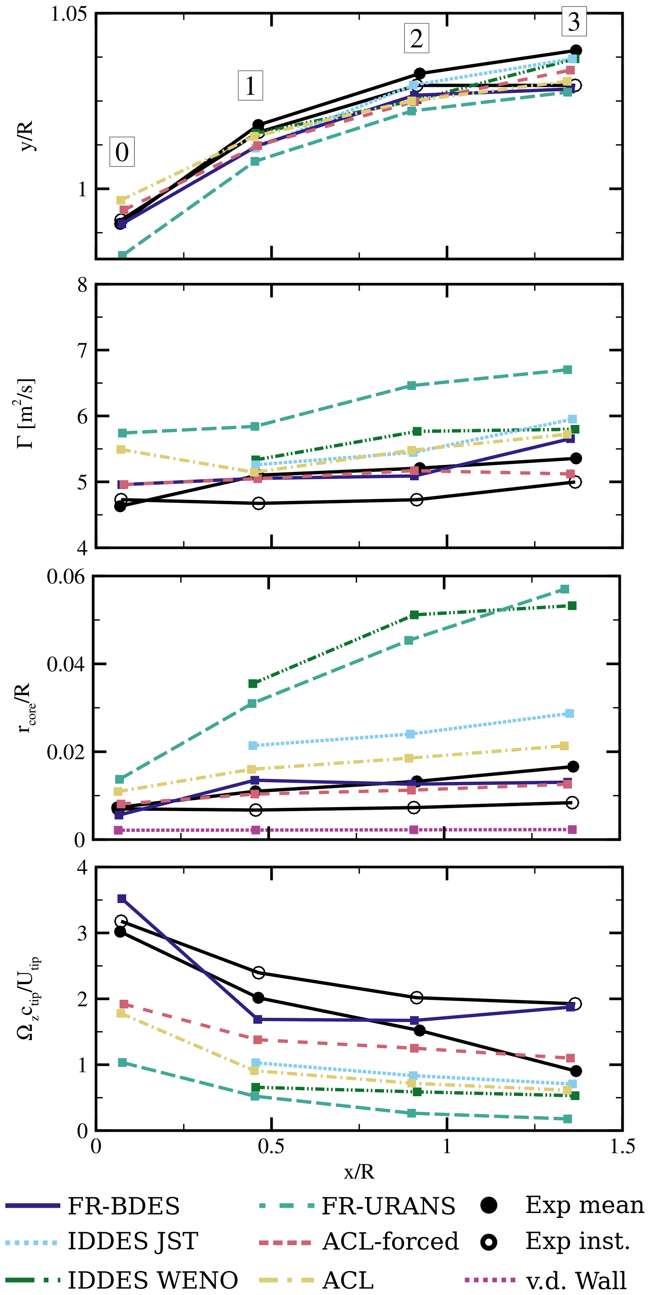
Figure 18 Comparison of the tip vortex properties between the PIV experiments of Schepers and Snel (2007), different simulation approaches, and the model of van der Wall et al. (2016). The IDDES-WENO and IDDES-JST results are reproduced from the Mexnext III contribution of the same authors.

The vortex core position depicted in the top graph of Fig. 18 is defined as the point of minimum out of the plane vorticity. Note that the scale of the y axis in the plot is 0.1 times smaller than that of the x axis. The vortex core position is adequately captured by the simulations, with the tendency of slightly underpredicting the wake expansion.

The circulation is calculated by integrating the vorticity within a circular area around the vortex core. The integration is executed by increasing the radii, until convergence is reached. This is equivalent to the closed line integration of the velocity vector according to the Stokes theorem and reads

$$\begin{array}{}\text{(2)}& \mathrm{\Gamma }=\underset{C}{\oint }\mathit{u}\cdot d\mathit{s}=\underset{A}{\int }\mathit{\omega }\cdot \mathit{n}\mathrm{d}A.\end{array}$$

The magnitude of the circulation is shown in the second panel from the top in Fig. 18. All simulations tend to overestimate the circulation, which confirms the general trend that most models overpredicted the lift near the blade tip. The overprediction is significantly larger for the RANS compared to the DES simulations. Towards vortex core 3, the uncertainty in the simulations increases. For example, the ACL-forced simulation, which showed very good agreement with its fully resolved counterpart for vortex 1 and vortex 2, predicts a decrease in the circulation, while the fully resolved simulation tends to result in an increase. The reason might be that in the fully resolved simulations and also in the PIV sheets, vorticity stemming from the shear layer, which wraps around the main tip vortex, is included in the integration.

The vortex core radius is crucial for assessing vortex preservation. Its accurate prediction is of special interest for example when it comes to wake–flight–vehicle interactions (Bühler et al., 2018; Tomaszewski et al., 2018; van der Wall et al., 2016; Cormier et al., 2020) or for investigations on the turbulent breakdown of the wake. The procedure in the evaluation tool of Meister (2015) follows the definition from Vollmers (2001), in which the vortex core is determined as half the distance between the peak values of the tangential velocity in a cross section through the vortex core. As expected from the previous analyses, the FR-URANS simulation strongly overestimates the vortex core radius by around a factor of 4. The wrong slope of the vortex growth emphasizes the excessive numerical diffusion.

In order to separate the effects of numerical dissipation and diffusion due to the turbulence model in DES-type simulations, we include our results presented in the Mexnext III project. This was conducted on a coarser mesh with about double grid spacing in the tip vortex area. Two IDDES simulations were performed, one with the second-order JST scheme using a dissipation coefficient k₄=128 and one with the higher-order WENO scheme. In the simulation with the JST scheme, even a larger core radius is obtained than with the FR-URANS simulation for vortex 1 and vortex 2. However, in the later stages, the gradient of the growth reduces, yielding an overall more concentrated tip vortex. The combination of DES with WENO clearly improves the results since the numerical dissipation from the convection scheme is reduced. The vortex is now only double the size of the experiments and reveals a very similar growth rate as in the phase-averaged PIV data. This means that numerical dissipation dominated the effect of the turbulence model and underlines that low-dissipation numerical schemes are a prerequisite to fully exploit the potential of scale-resolving simulation techniques. In the present FR-BDES and ACL-forced simulations, the vortex diameter is significantly reduced. It is of the order of the phase-averaged PIV measurements but still larger compared to the instantaneous PIV evaluation. The semi-empirical van der Wall model predicts even smaller core radii than the instantaneous PIV results. This trend was also observed in Cormier et al. (2020), where it was compared to measurements and CFD simulations on a multi-megawatt turbine.

Turning finally to the maximum of the vorticity based on the maximum value found in the core region, we observe a very similar trend to that of the core radius. The FR-URANS solution severely underestimates the core vorticity. A clear improvement is obtained with DES as the eddy viscosity is effectively reduced. As observed before, the use of a higher-order scheme is beneficial for preserving the velocity gradients in the core. The FR-BDES simulation yields the most accurate results, predicting even a larger vorticity than the experiments for the initial core of vortex 0. The smearing of the forces in the ACL-type simulation already leads to a reduction in the vorticity. Due to the coarsening of the grid size from vortex 0 to vortex 1, the vorticity drops below the experimental values for all numerical approaches but recovers for the FR-BDES until vortex 3. At that position, there is also a significant difference among the experimental results. The averaged data show an almost-linear decrease in the vorticity, whereas in the instantaneous fields the slope decreases with the streamwise distance. The reason is that with the averaging, small-scale vortex motions (vortex jittering or wandering) decrease their sharpness when looking at them in a time-averaged frame.

Compared to numerical wake simulations found in the literature and described in Sect. 1, the FR-BDES simulation significantly improves the prediction capabilities of tip vortices of wind turbine wakes because it combines several methodological extensions, namely a higher-order numerical scheme in combination with the BDES turbulence modeling approach that results in almost-implicit LES behavior in flows of solid rotation. This feature in the DES model is based on the use of the σ velocity gradient operator (Mockett et al., 2015), which does not contribute to the eddy viscosity in the case of pure rotation. Therefore, it is effective in reducing the diffusivity in the tip vortex core region.

It can be summarized, also by our own experiences, that with the URANS approach, successive grid refinement and the usage of low-dissipation numerical schemes can reduce the vortex core diameter to a certain extent. However, the slope of the vortex growth in particular was always highly overpredicted, which would result in inadequate predictions, for example of wake breakdown. Accurate predictions of blade tip vortices therefore require sufficient grid resolution and an adapted time step, as well as a turbulence model that does not erroneously damp the velocity gradients within the tip vortices. These methods further benefit from utilizing higher-order convection schemes. Whether an actuator line method or geometrically fully resolved blade simulations are employed plays only a subordinate role, as long as the very early stages of the tip vortex development are not of interest.

6 Conclusions

A computational study was conducted on the near wake and tip vortex development of the MEXICO model wind turbine operating in stalled conditions at a low tip-speed ratio. Different simulation methodologies were compared with experimental data from PIV. One focus was on comparing the traditional URANS approach with a recently developed variant of the detached-eddy simulation technique. The second emphasis was on comparing the modeling of the rotor. In this comparison, the actuator line method was juxtaposed with the simulation of the geometrically fully resolved turbine. Two approaches were pursued for the actuator line simulation. The effects were isolated to the propagation of the injected forces by transferring them from the full-resolution simulation to eliminate the uncertainties in the BEM and the polars and comparing these results to a standard actuator line with internal force calculation.

The following conclusions can be drawn from this study:

1. The URANS turbulence modeling approach is sufficiently accurate to predict the mean velocity distribution in the near wake governing the induction of the rotor. Expectedly, no interaction between turbulent structures in the blade wake was resolved. Also, the flow in the region of the root vortex remained coherent. The tip vortex size was tremendously overpredicted, although sufficient grid resolution and a higher-order numerical scheme were provided. The URANS approach is nonetheless sufficiently accurate in predicting the mean induction effects of the blade wake. It can therefore still be recommended for practical applications focusing on the mean flow field of the near wake, even in the separated flow regime.

2. The scale-resolving simulation using the Bernoulli-based DES formulation on the geometrically fully resolved rotor captured the details of the turbulent flow field in the vicinity of the blade, showing very good agreement regarding the shape and sizes of the structures. At the scale of the rotor wake, the axial velocity traverses were also found to coincide well with the experiments. The vortex core diameter agreed well with the phase-averaged PIV results but was still overpredicted relative to the instantaneous fields. Moreover, secondary vortices around the main tip vortex could be captured. The formation of these structures as well as the dynamics of the tip vortex motion will be investigated in detail in a second paper (part 2).

3. In the standard actuator line approach with forces calculated from the blade-element momentum theory based on uncorrected two-dimensional polars, the agreement of the loads in the outer blade area was reasonably accurate. In the inner half of the rotor they were substantially underestimated. This resulted in the formation of an incorrect wake topology in the inboard region, where the axial and tangential blade inductions were predicted to be far too low. Also, the trailing vortices in the middle part of the radius were not captured since the gradients in bound circulation could emerge out of the forces stemming from the two-dimensional polars. In the outer region of the wake, the results were comparable to those of the fully resolved simulations. As a consequence, the tip vortices and their propagation were also captured reasonably well.

4. It could be shown that by injecting the “correct” forces from the scale-resolving simulations with geometrically resolved blades, the same bound circulation could be proven as in the donor simulation. This way, the method of the force projection could be verified in a clear way. As a result of the agreement in the circulation, there was also very good agreement between the two simulations with respect to the mean velocity field, the tip vortex diameter and the mixing process of the root vortex in the inner region of the blade. However, since only the trailing vortices can be resolved in the ACL, the development of the blade wake remained more coherent, and its breakdown was delayed.

5. Overall, it can be concluded that the ACL method can also be used in massively separated flows. However, it is highly important to impose forces which represent the actual three-dimensional flow phenomena as good as possible. Although it was not explicitly shown in this study, the application of a model for rotational augmentation is highly recommended. A comparison with corresponding correction models could be the subject of future research.