Swell impacts on an offshore wind farm in stable boundary layer: wake flow and energy budget analysis

We investigate the impact of swell on wind turbine wakes and the power output of offshore wind farms under stable atmospheric conditions. We conduct large-eddy simulations, and the influence of swell is modeled by incorporating a wave-induced stress term in the momentum equation. We perform kinetic energy budget analysis, including all relevant source and sink terms. Two typical scenarios in the North Sea area with modest wind speeds and wind-following and wind-opposing fast waves are considered. The results show that swells significantly affect the wind speed profiles and turbulence intensity across the entire operational height of the wind turbines. The impact of the swell predominantly affects the inflow, while its significance progressively diminishes downstream. From kinetic energy budget analysis, we discover that the wave effects are primarily exerted through indirect modification of the advection of energy in the streamwise and vertical dimensions instead of the direct wave-induced energy input/output. The wind shift and yawing adjustment caused by waves play a crucial role in the energy harvesting rate, depending on the specific inflow direction and wind farm layout. The relative changes in total power production reach up to 20.0 %/−27.3 % for the wind-following and wind-opposing wave scenarios, respectively.

1 Introduction

As a substantial and environmentally friendly energy resource, offshore wind energy offers a promising opportunity to mitigate climate change and accelerate the global energy transition from fossil fuels toward sustainable energy sources. Offshore wind exhibits different characteristics from its counterpart over land due to the ubiquitous and changeable wind–wave interactions at the air–sea interface, which significantly influences the airflow above through complex physical processes such as velocity and pressure perturbations and wave breaking and spray (Sullivan and McWilliams, 2010). As the offshore wind industry is expected to experience rapid growth in the near future, it is crucial to enhance our understanding of marine atmospheric boundary layer (MABL) characteristics and their impacts on the performance of offshore wind farms.

Numerous observational studies have provided evidence supporting the significant dependence of atmosphere–ocean coupling on wind–sea conditions (Donelan et al., 1997; Drennan et al., 2003; Smedman et al., 2003). The wind–sea condition is usually quantified by wave age, defined as the ratio of the wave phase speed to the wind speed at 10 m height (or friction velocity), and categorized into two regimes: wind wave (young sea) and swell (old sea). Wind waves are generated by local winds, transferring energy from the atmosphere to the ocean (Jenkins et al., 2012). They typically align with the wind direction and are characterized by relatively short wavelengths and low wave heights, with their strength determined by the wind's duration and fetch. Swells, on the other hand, are waves originating from distant weather systems and have traveled away from their source. These waves are characterized by longer wavelengths, greater amplitudes, and higher propagation speeds than wind–sea waves. Therefore, swells typically possess higher energy and are associated with more complex physical processes. These processes include the upward transfer of momentum flux (Grachev and Fairall, 2001; Kahma et al., 2016), the occurrence of low-level jets (Hanley and Belcher, 2008; Semedo et al., 2009), and surface stresses misaligned with the wind (Zou et al., 2019; Patton et al., 2019; Chen et al., 2020a). The impact of swell on the wind field is particularly pronounced under stable atmospheric conditions, where buoyancy suppresses turbulence, allowing wave-induced flow structures to dominate near the ocean surface (Zou et al., 2018; Jiang, 2020). Furthermore, a statistical analysis based on data from the 45-year European Centre for Medium-Range Weather Forecasts reanalysis (ERA-40) revealed that swells prevail across the global ocean (Semedo et al., 2011).

The computational fluid dynamics (CFD) technique plays a crucial role in analyzing wind farm performance in offshore environments, primarily due to its unparalleled ability to provide detailed three-dimensional flow data. This level of detail is crucial for comprehending the complex dynamics of wind farm airflow, facilitating advancements in wind energy engineering models, including the development of more accurate reduced-order and surrogate models (Breton et al., 2017). Previous large-eddy simulation (LES) studies on offshore wind farms have generally employed two approaches to model wave effects: the wave-averaged method and the wave-phase-resolved method (Deskos et al., 2021). The wave-averaged approach, often employing Monin–Obukhov similarity theory (MOST) with a roughness length near the ocean surface (Wu and Porté-Agel, 2015; Dörenkämper et al., 2015; Sood et al., 2022), is less effective under old-sea conditions (Liu et al., 2022) and cannot capture swell-induced upward momentum fluxes (Wu and Qiao, 2022; Ning et al., 2023). In contrast, wave-phase-resolved LES incorporates surface geometry via coordinate transformation, enabling detailed simulations of wind–wave interactions. For example, Yang et al. (2014) demonstrated how swell modifies wind profiles and turbulence intensity (TI), influencing wake recovery and power production. Using similar solvers, Yang et al. (2022b) and Xiao and Yang (2019) investigated the influence of swell propagation speed, direction, and swell-induced pitch motion on offshore wind farm performance. However, wave-phase-resolved simulations are computationally expensive due to the need for mesh transformation and finer temporal and spatial resolutions, limiting their application to large-scale wind farms. Recent efforts have explored intermediate approaches between wave-averaged and wave-phase-resolved methods. For instance, the wave drag model proposed by Aiyer et al. (2023, 2024) offers a balance between accuracy and computational cost, while machine-learning-based models by Zhang et al. (2023) and Yousefi et al. (2024) show promise in capturing wave effects efficiently.

With the expansion of offshore wind farms and the emergence of wind farm clusters, new flow phenomena have been observed, including the blockage effect (Sanchez Gomez et al., 2023), gravity wave influences (Allaerts and Meyers, 2018), atmospheric pressure gradient changes (Antonini and Caldeira, 2021), and wind farm wake deflection (van der Laan and Sørensen, 2017). Exploring the influence of wind–wave interactions on these large-scale wind farm characteristics opens up a compelling research field. Bakhoday-Paskyabi et al. (2022) evaluated the performance of online and offline wind–wave coupling in mesoscale and microscale modeling frameworks during typical events such as low-level jets (LLJs) and open cellular convection (OCC), establishing a close model chain for meso-to-micro downscaling and wind-turbine-scale process analysis. Porchetta et al. (2021) simulated 1250 turbines using the WRF and WRF-SWAN models, showing a difference in power output of up to 20 % and a 25 % variation in wake length with dynamic wave effects. Despite this, microscale research on the role of waves, particularly swells, in shaping the dynamics of large-scale wind farm flows remains limited. Bridging this gap requires the development of robust, generalizable wave modeling techniques that effectively capture the interactions between waves and MABL flows while overcoming the computational challenges associated with large-scale offshore wind farm simulations.

In this study, we integrate a novel wave-induced stress parameterization method into a LES code to simulate a large-scale offshore wind farm under a stable atmospheric boundary layer with low wind speed and fast swells. Our objective is to investigate the impacts of swells on the performance of the wind farm and its wake flow. In particular, we aim to uncover the underlying mechanisms by closely examining the conservation of kinetic energy. The paper is organized as follows: Sect. 2 describes the modeling tool, wave parameterization method, and detailed configuration. Section 3 presents the modeling results and their analysis. The findings of this study are summarized and concluded in Sect. 4.

2 Methods

2.1 LES model

In our study, we utilize the Parallelized Large-Eddy Simulation Model (PALM), an open-source LES code developed by the PALM group at Leibniz University Hanover (Maronga et al., 2020). This code is written in Fortran language and specifically designed for massively parallel computing tasks. It solves the incompressible Navier–Stokes (N–S) equations as follows:

$$\begin{array}{}\text{(1)}& {\displaystyle \frac{\partial u_j}{\partial x_j}}=\mathrm{0},\text{(2)}& {\displaystyle }\begin{array}{rl}{\displaystyle \frac{\partial u_i}{\partial t}}& =-{\displaystyle \frac{\partial u_i{u}_j}{\partial x_j}}-{\mathit{ϵ}}_{ijk}{f}_j{u}_k+{\mathit{ϵ}}_{i\mathrm{3}k}{f}_{\mathrm{3}}{u}_{g,k}\\ & -{\displaystyle \frac{\mathrm{1}}{{\mathit{\rho }}_{\mathrm{a}}}}{\displaystyle \frac{\partial {\mathit{\pi }}^{*}}{\partial x_i}}+g{\displaystyle \frac{\mathit{\theta }-\langle \mathit{\theta }\rangle }{\langle \mathit{\theta }\rangle }}{\mathit{\delta }}_{i\mathrm{3}}+{\displaystyle \frac{\partial {\mathit{\tau }}_{\text{SGS},ij}}{\partial x_j}}+{\displaystyle \frac{\partial {\mathit{\tau }}_{\mathrm{w},ij}}{\partial x_j}}+S_i.\end{array}\end{array}$$

Here, t denotes time; u_i, u_j, and u_k are the velocity components; π^* is the modified perturbation pressure; and θ represents potential temperature with horizontal averaging indicated by angular brackets. The subgrid-scale (SGS) turbulent stress τ_SGS,ij is parameterized by the 1.5-order Deardorff subgrid-scale model (Deardorff, 1980). The Coriolis parameter $f=(\mathrm{0},\mathrm{2}\mathrm{\Omega }\cos \mathit{\varphi },\mathrm{2}\mathrm{\Omega }\sin \mathit{\varphi })$ involves Earth's angular velocity $\mathrm{\Omega }=\mathrm{0.729}\times {\mathrm{10}}^{-\mathrm{4}}$ rad s⁻¹, and latitude ϕ is set at 54° (corresponding to the position of the studied wind farm). Gravitational acceleration is g=9.81 m s⁻², and ρ_a represents dry air density. ϵ and δ denote the Levi-Civita symbol and Dirac delta function, respectively. S_i represents the momentum sink term by wind turbines. These terms align with the original governing equations in Maronga et al. (2015). However, we introduce an additional term τ_w,ij to denote wave-induced stress, detailed in the subsequent section. Time advancement uses the third-order Runge–Kutta method, and spatial discretization employs a staggered grid with the fifth-order Wicker–Skamarock scheme for advection.

2.2 Parameterization of wave-induced stress

The wave-induced stress at the ocean surface, τ_w(0), is derived by dividing the energy transfer rate between the wind and wave fields by the wave speed, $c=\mathit{\omega }/k$, and integrating this value over the wave spectrum (Hanley and Belcher, 2008):

$$\begin{array}{}\text{(3)}& {\mathit{\tau }}_{\mathrm{w}}\left(\mathrm{0}\right)=-{\displaystyle \frac{{\mathit{\rho }}_{\mathrm{w}}}{{\mathit{\rho }}_{\mathrm{a}}}}g\underset{\mathrm{0}}{\overset{\mathrm{2}\mathit{\pi }}{\int }}\underset{\mathrm{0}}{\overset{{\mathit{\omega }}_{\mathrm{c}}}{\int }}{\displaystyle \frac{\mathit{k}}{w}}\mathit{\beta }E(\mathit{\omega },{\mathit{\varphi }}_{\mathrm{w}})\mathrm{d}\mathit{\omega }\mathrm{d}{\mathit{\varphi }}_{\mathrm{w}},\end{array}$$

where ρ_w represents the density of water, ϕ_w is the wave propagation direction, ω denotes the wave angular frequency, and k is the wave number vector. E(ω,ϕ_w) represents the wave spectrum function, and β, the wave damping rate, is calculated using the formulas from Ardhuin et al. (2010):

$$\begin{array}{}\text{(4)}& \mathit{\beta }=\left\{\begin{array}{ll}{\displaystyle \frac{{\mathit{\rho }}_{\mathrm{a}}}{{\mathit{\rho }}_{\mathrm{w}}}}\left(\mathrm{2}k\sqrt{\mathrm{2}\mathit{\nu }\mathit{\omega }}\right)& \mathit{Re}<{\mathit{Re}}_{\mathrm{c}}\\ {\displaystyle \frac{{\mathit{\rho }}_{\mathrm{a}}}{{\mathit{\rho }}_{\mathrm{w}}}}(\mathrm{16}{f}_e{\mathit{\omega }}^{\mathrm{2}}{u}_{\text{orb}}/g)& \mathit{Re}\ge {\mathit{Re}}_{\mathrm{c}}\end{array}\right..\end{array}$$

Here f_e is a constant coefficient set to 0.008. The boundary Reynolds number, Re, is defined as $\mathit{Re}=\mathrm{2}{u}_{\text{orb}}{H}_{\mathrm{s}}/\mathit{\nu }$, where ν is the kinematic viscosity of air, and H_s represents the significant wave height. The surface orbital velocity, u_orb, is calculated as $u_{\text{orb}}=\sqrt{m_{\mathrm{2}}/\left(\mathrm{2}{m}_{\mathrm{0}}\right)}{H}_{\mathrm{s}}$, with m₀ and m₂ denoting the zeroth and second moments of the wave spectrum, respectively. The critical Reynolds number, Re_c, used to differentiate between the viscous and turbulent states of flow near the surface, is defined as ${\mathit{Re}}_{\mathrm{c}}=\mathrm{2.0}\times {\mathrm{10}}^{\mathrm{5}}/H_{\mathrm{s}}$. The wave spectrum in the present work is defined as the empirical wave spectrum proposed by Donelan et al. (1985) multiplied by an exponential factor:

$$\begin{array}{}\text{(5)}& \begin{array}{rl}& S\left(\mathit{\omega }\right)={\displaystyle \frac{\mathit{\alpha }{g}^{\mathrm{2}}}{{\mathit{\omega }}^{\mathrm{4}}{\mathit{\omega }}_p}}\exp [-{\left({\displaystyle \frac{{\mathit{\omega }}_p}{\mathit{\omega }}}\right)}^{\mathrm{4}}]{\mathit{\gamma }}^r\exp \left[{\left({\displaystyle \frac{\mathit{\omega }}{{\mathit{\omega }}_{\mathrm{0}}}}\right)}^{\mathrm{3}}\right],\\ & r=\exp [-{\displaystyle \frac{(\mathit{\omega }-{\mathit{\omega }}_p{)}^{\mathrm{2}}}{\mathrm{2}{\mathit{\sigma }}^{\mathrm{2}}{\mathit{\omega }}_p^{\mathrm{2}}}}],\end{array}\end{array}$$

where

$$\begin{array}{}\text{(6)}& \begin{array}{rl}& \mathit{\alpha }=\mathrm{0.006}{\left({\displaystyle \frac{U_{\mathrm{10}}}{c_p}}\right)}^{\mathrm{0.55}},\mathit{\gamma }=\mathrm{1.7}+\mathrm{6.0}\log \left({\displaystyle \frac{U_{\mathrm{10}}}{c_p}}\right),\\ & \mathit{\sigma }=\mathrm{0.08}[\mathrm{1.0}+\mathrm{4.0}{\left({\displaystyle \frac{c_p}{U_{\mathrm{10}}}}\right)}^{\mathrm{3}}].\end{array}\end{array}$$

Here, ω_p is the peak wave frequency, c_p refers to the peak phase speed, and U₁₀ denotes the wind speed at 10 m height. ${\mathit{\omega }}_{\mathrm{0}}^{-\mathrm{3}}$ within the exponential factor is set to −0.01 following Hanley and Belcher (2008). This setting helps to approximate a swell-dominated wave spectrum, characterized by the dampening of high-frequency components due to dissipation over long distances. We employ a theoretical directional spectrum, expressed as

$$\begin{array}{}\text{(7)}& D\left({\mathit{\varphi }}_{\mathrm{w}}\right)={\displaystyle \frac{\mathrm{1}}{\mathit{\pi }}}{\cos }^{\mathrm{2}}\left({\displaystyle \frac{{\mathit{\varphi }}_{\mathrm{w}}-{\mathit{\varphi }}_{\mathrm{w},p}}{\mathrm{2}}}\right),\end{array}$$

to characterize the directional distribution of wave energy, where ϕ_w,p represents the peak wave propagation direction. The directional wave spectrum is then calculated by multiplying Eq. (5) by Eq. (7), resulting in $E(\mathit{\omega },{\mathit{\varphi }}_{\mathrm{w}})=S\left(\mathit{\omega }\right)D\left({\mathit{\varphi }}_{\mathrm{w}}\right)$. We define a critical frequency as in Semedo et al. (2009), ω_c, which demarcates the boundary between swell and wind wave in the frequency domain, calculated as ${\mathit{\omega }}_{\mathrm{c}}=g/U_{\mathrm{10}}$. The integration is performed within the range $\mathrm{0}<\mathit{\omega }<{\mathit{\omega }}_{\mathrm{c}}$ to explicitly calculate the momentum fluxes from swells to the wind field, while higher-frequency wave contributions, only acting as surface drag, are accounted for using the roughness length. Assuming that the wind and wave conditions are consistent across the domain, the wave-induced stress is treated as horizontally homogeneous, thereby making it a function dependent exclusively on height. Moreover, numerous researchers have observed that wave-induced stress decreases exponentially with height (Högström et al., 2015; Wu et al., 2018). Therefore, we approximate the vertical profile of τ_w by multiplying its surface value by an exponential decay function:

$$\begin{array}{}\text{(8)}& {\mathit{\tau }}_{\mathrm{w}}\left(z\right)={\mathit{\tau }}_{\mathrm{w}}\left(\mathrm{0}\right)e^{-a\widehat{k}z},\widehat{k}={\displaystyle \frac{{\int }_{\mathrm{0}}^{\mathrm{2}\mathit{\pi }}{\int }_{\mathrm{0}}^{{\mathit{\omega }}_{\mathrm{c}}}kE(\mathit{\omega },{\mathit{\varphi }}_{\mathrm{w}})\mathrm{d}\mathit{\omega }\mathrm{d}{\mathit{\varphi }}_{\mathrm{w}}}{{\int }_{\mathrm{0}}^{\mathrm{2}\mathit{\pi }}{\int }_{\mathrm{0}}^{{\mathit{\omega }}_{\mathrm{c}}}E(\mathit{\omega },{\mathit{\varphi }}_{\mathrm{w}})\mathrm{d}\mathit{\omega }\mathrm{d}{\mathit{\varphi }}_{\mathrm{w}}}},\end{array}$$

where a=1.0 is the decay coefficient, and $\widehat{k}$ is the integration-weighted average wave number. Readers are referred to our previous work (Ning and Paskyabi, 2024) for a comprehensive explanation of the proposed wave model and the determination of its parameters.

2.3 Wall-stress model

In our simulation, we utilize a wall-stress model that assumes a constant flux layer (CFL) near the surface to estimate momentum fluxes at the bottom of the model domain. This model differs from LES wall-stress models based on the conventional Monin–Obukhov similarity theory (Monin and Obukhov, 1954), as it accounts for not only viscous stress τ_ν and turbulent stress τ_t but also the stress arising from wind–wave interaction τ_w (Paskyabi et al., 2014), i.e.,

$$\begin{array}{}\text{(9)}& {\mathit{\tau }}_{\text{tot}}={\mathit{\tau }}_{\mathit{\nu }}+{\mathit{\tau }}_{\mathrm{t}}+{\mathit{\tau }}_{\mathrm{w}}.\end{array}$$

The sum of the viscous and turbulent stresses can be approximated by the viscosity model within the height of 10 m (Chen et al., 2020b):

$$\begin{array}{}\text{(10)}& {\mathit{\tau }}_{\text{tot}}-{\mathit{\tau }}_{\mathit{\nu }}-{\mathit{\tau }}_{\mathrm{w}}=K_{\mathrm{m}}{\displaystyle \frac{\mathrm{d}\mathit{u}\left(z\right)}{\mathrm{d}z}},z<\mathrm{10.0}\mathrm{m},K_{\mathrm{m}}=\mathit{\kappa }z{u}_{*},\end{array}$$

where K_m is the momentum eddy diffusivity. It is parameterized to be linearly proportional to both the height and the friction velocity $u_{*}=\sqrt{\left|{\mathit{\tau }}_{\text{tot}}\right|}$, with κ=0.4 representing the von Kármán constant. Furthermore, the viscous stress τ_ν is omitted here because it is only important in the millimeter above the surface (Hanley and Belcher, 2008; Semedo et al., 2009). Integrating Eq. (10) yields the vertical velocity profile within the constant flux layer:

$$\begin{array}{}\text{(11)}& \mathit{u}\left(z\right)={\displaystyle \frac{{\mathit{\tau }}_{\text{tot}}}{\mathit{\kappa }{u}_{*}}}[\ln {\displaystyle \frac{z}{z_{\mathrm{0}}}}-{\mathrm{\Psi }}_{\mathrm{m}}({\displaystyle \frac{z}{L}}\left)\right]-\underset{z_{\mathrm{0}}}{\overset{z}{\int }}{\displaystyle \frac{{\mathit{\tau }}_{\mathrm{w}}\left(z\right)}{\mathit{\kappa }z{u}_{*}}}\mathrm{d}z.\end{array}$$

Here, the roughness length is determined using Charnock's method (Charnock, 1955) as $z_{\mathrm{0}}={\mathit{\alpha }}_{\mathrm{c}}{u}_{*}^{\mathrm{2}}/g$, where α_c=0.012 is the Charnock coefficient. The first term on the right-hand side of Eq. (11) aligns with the MOST-based logarithmic wind profile, while the second term represents the adjustment to wind velocity due to the influence of swells. ${\mathrm{\Psi }}_{\mathrm{m}}(z/L)$ represents the integrated universal stability function, which depends on height normalized by the Monin–Obukhov length, L (Van Wijk et al., 1990). Figure 1 provides a flowchart illustrating the integration of the wave model into the LES code. Equation (11) is solved at z=10 m to determine the total surface stress, τ_tot, and the friction velocity, u_*, for each grid point. At every time step, the wind velocity u(z=10) is known, and the wave-induced stress, τ_w, is explicitly calculated using Eq. (3). The value of u_* from the previous time step is used as an initial guess to iteratively solve for τ_tot, u_*, z₀, and L until Eq. (11) is satisfied. The resulting total surface stress is then applied as the wall-stress boundary condition, while the vertical divergence of the wave-induced stress is calculated and incorporated into the momentum equation, Eq. (2). The simulation then progresses to the next time step.

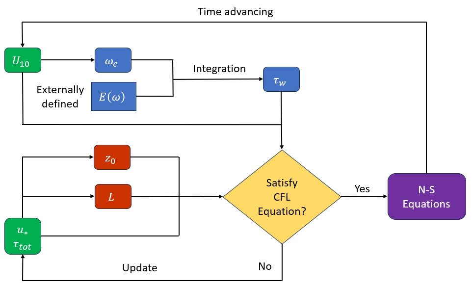
Figure 1 Flowchart of wall-stress model with wave parameterization based on constant flux layer assumption.

2.4 Simulation setup

In this study, we focus on a specific wind farm within a cluster situated approximately 60 km north of the German coast in the North Sea. This wind farm, located at 54°30^′ N, 6°22^′ E, as indicated in Fig. 2, consists of 80 wind turbines, each with a capacity of 5 MW. The wind turbines are represented by the Actuator Disk Model with Rotation (ADM-R), as detailed in Wu and Porté-Agel (2015). We utilize the design parameters of the benchmark NREL-5 MW wind turbine (Jonkman et al., 2009), which include a rotor diameter of D=126.0 m, a hub height of 90 m, and a rated wind speed of 11.4 m s⁻¹.

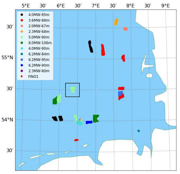
Figure 2 Locations of wind farms in the North Sea.

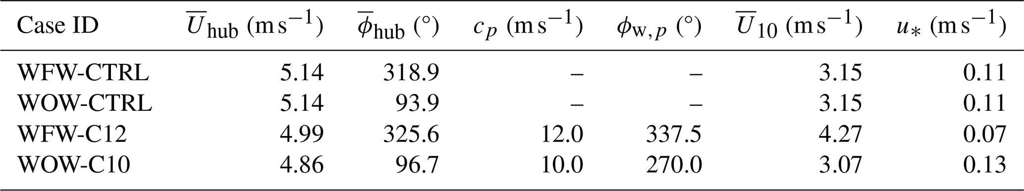
We first perform precursor simulations of stable ABL flows without any wind farms. We are interested in the regime characterized by moderate wind speeds coupled with fast-propagating waves, a scenario where the influence of swells is relatively pronounced as reported by Chen et al. (2019) and Zou et al. (2019). This choice of setup was widely used in previous numerical studies of the impact of swells on the marine atmospheric boundary layer (Sullivan et al., 2008; Nilsson et al., 2012; Jiang et al., 2016). Wind and wave data, collected from the FINO1 platform (indicated by a red star in Fig. 2) between May 2015 and April 2016, are presented as rose diagrams in Fig. 3. The diagrams show that low to moderate wind speeds (represented by the dark blue region) primarily originate from the northwest and east, and fast peak wave speeds (indicated by the dark-red region) most frequently come from the west and north-northwest. Drawing from this data, two distinct scenarios are chosen for our analysis: (1) a northwest wind with a hub height speed of 5.0 m s⁻¹, accompanied by waves originating from a 337.5° direction and having a peak phase speed of 12.0 m s⁻¹, representing the wind-following wave (WFW) condition, and (2) an easterly wind of 5.0 m s⁻¹, coupled with oppositely propagating waves from west to east at a speed of 10.0 m s⁻¹, as the wind-opposing wave (WOW) condition. These two cases are labeled as WFW-C12 and WOW-C10, respectively. The wind–wave conditions and corresponding model parameters for the various cases are summarized in Table 1.

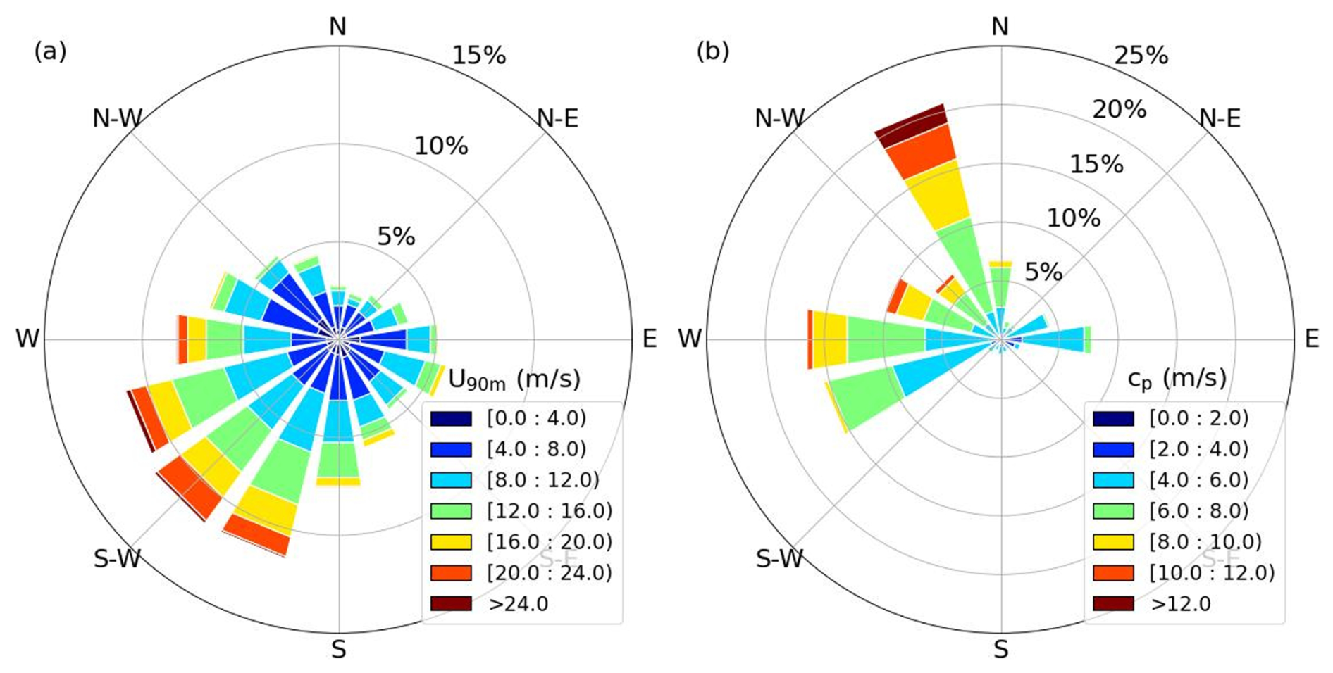
Figure 3 Rose diagrams of wind (a) and wave (b) in the FINO1 area, covering the period from May 2015 to April 2016.

Table 1 Abbreviations and setups for main runs.

The computational domain for the preruns is set with a uniform horizontal grid size of ${\mathrm{\Delta }}_x={\mathrm{\Delta }}_y=\mathrm{6}$ m. This grid resolution is considered sufficiently fine according to Sanchez Gomez et al. (2023). Vertically, the grid size is Δ_z=6 m up to a height of 216 m, above which it increases regularly at a rate of 1.036, reaching the domain top at 4.6 km with a maximum Δ_z of 48 m. The initial temperature profile is structured in three segments: a constant 300.0 K from the ocean surface to 1000 m; a steep capping inversion up to 1200.0 m, increasing at 1.0 K per 100.0 m; and then a gradual rise by 0.1 K per 100.0 m up to the top of the boundary layer. A Rayleigh damping layer is set above z=1000.0 m to avoid the reflection of gravity waves at the upper boundary (Klemp et al., 2008). Each prerun spans 48 h, with the first 36 h dedicated to establishing a fully developed neutral flow, followed by 12 h of constant surface cooling at a rate of −0.08 K h⁻¹ to produce a weakly stable boundary layer. The wave model is activated at 45 h and gradually reaches the full swell-induced stress, as determined by Eq. (3), over a 2 h linear relaxation period. This approach ensures numerical stability and helps mitigate inertial oscillations. Additionally, two control cases (WFW-CTRL and WOW-CTRL) are conducted to isolate and analyze the specific impacts of swells. These control cases exclude the wave parameterization method and instead use a constant roughness length of $z_{\mathrm{0}}=\mathrm{2}\times {\mathrm{10}}^{-\mathrm{4}}$ to account for the total surface stress.

Once a quasi-steady stable boundary layer flow is established in the preruns, the flow data are used to initialize the so-called main runs, which incorporate the wind farm. These main runs retain the same mesh resolution, temperature profile, and wind–wave conditions as the preruns. However, the domain size is expanded to ensure adequate simulation of the flows within and around the entire wind farm, as illustrated in Fig. 4. To better utilize the domain, the x axes are aligned with the hub height wind direction, ensuring a consistent left-to-right wind flow in all cases. To maintain the turbulent inflow and its equilibrium with the mean wind shear and stability conditions, velocity fluctuations are continuously recycled in the region extending from $\mathrm{0}<x<\mathrm{1.5}$ km. The cyclic condition is applied to the crosswise boundaries, and the outflow radiation condition is used at the outlet boundary. The wind turbines, positioned based on their real-world locations, are arranged in a right-angled trapezoidal layout within the computational domain. In the WFW-CTRL and WFW-C12 cases, as in Fig. 4a, the wind originates from the northwest. Consequently, the x axis is rotated clockwise by 45° from the east to align with the wind direction. The wind farm layout is adjusted accordingly: the turbine located at the northwest corner becomes the foremost in the windward direction, and the subsequent turbines are arrayed in a staggered, diagonal formation behind it, with spacings of approximately 1.1 km in both the streamwise and crosswise directions. In the WOW-CTRL and WOW-C10 cases (Fig. 4b), the wind direction is easterly. Here, the turbines are arranged in columns that run west to east in line with the wind flow, with a streamwise spacing of 0.9 km. The crosswise spacings along the south–north rows are around 0.7 km. In both domains, a 5 km (40D) buffer is set between the inlet boundary and the wind farm to encompass the wind induction zone. Additionally, a 10–12 km fetch (80D–95D) is allocated beyond the wind farm to the outlet boundary, ensuring sufficient space for wake flow development and recovery.

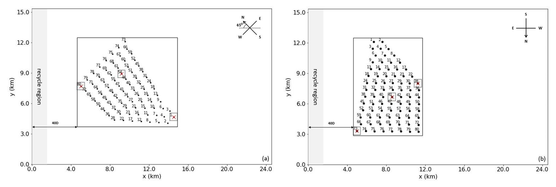
Figure 4 Top view of the computational domains for the main runs: wind-following wave scenario (a), wind-opposing wave scenario (b).

All main runs span a duration of 3 h of physical time, which is nearly twice the time required for the wake to traverse the domain. Figure 5 illustrates the temporal evolution of the friction velocity u_* from t=36 h, when surface cooling is initiated, to the end of the main runs. The friction velocity initially undergoes a gradual decline as the surface cools and stabilizes after approximately 6 h. The introduction of wind-following or wind-opposing waves subsequently reduces or increases u_*, respectively, until a new steady state is reached, marked by a plateau in the time series during the last 2 h of the main runs. The shaded gray region indicates the final hour of the main runs, during which data are averaged and used for the subsequent analysis.

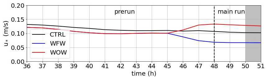
Figure 5 Temporal evolution of horizontally averaged friction velocity during the preruns (final 12 h) and main runs. The shaded region represents the last hour of the main runs, from which the data used for analysis are extracted.

2.5 Kinetic energy budget

The kinetic energy (KE) of airflow, representing the energy due to its motion, is the direct energy source for wind turbines. Understanding kinetic energy is vital for elucidating the dynamics of the marine atmospheric boundary layer, particularly its interactions with offshore wind farms and the ocean surface beneath. In this study, we conduct an in-depth kinetic energy budget analysis to reveal the physical processes responsible for the generation, redistribution, and dissipation of KE for the wind field inside the offshore wind park, with a special focus on the role of swells in KE conservation.

The mean kinetic energy consists of the kinetic energy of the mean flow (KEM) and the turbulent kinetic energy (TKE):

$$\begin{array}{}\text{(12)}& {\stackrel{\mathrm{‾}}{E}}_k=\stackrel{\mathrm{‾}}{E}+\stackrel{\mathrm{‾}}{e}={\displaystyle \frac{\mathrm{1}}{\mathrm{2}}}({\stackrel{\mathrm{‾}}{u}}_i{\stackrel{\mathrm{‾}}{u}}_i+\stackrel{\mathrm{‾}}{u_i^{\prime }{u}_i^{\prime }}).\end{array}$$

Here the prime denotes the turbulent component. The conservation equation for the mean kinetic energy can be derived by multiplying Eq. (2) by u_i and taking the time average:

$$\begin{array}{}\text{(13)}& \begin{array}{rl}{\displaystyle \frac{\partial {\stackrel{\mathrm{‾}}{E}}_k}{\partial t}}=& \underset{A}{\underbrace{-{\displaystyle \frac{\partial {\stackrel{\mathrm{‾}}{u}}_k{\stackrel{\mathrm{‾}}{E}}_k}{\partial x_k}}}}\underset{T}{\underbrace{-{\displaystyle \frac{\partial {\stackrel{\mathrm{‾}}{u}}_i\stackrel{\mathrm{‾}}{u_k^{\prime }{u}_i^{\prime }}}{\partial x_k}}+{\displaystyle \frac{\partial \stackrel{\mathrm{‾}}{u_i{\mathit{\tau }}_{\text{ki}}}}{\partial x_k}}-{\displaystyle \frac{\partial \stackrel{\mathrm{‾}}{u_k^{\prime }e}}{\partial x_k}}-{\displaystyle \frac{\mathrm{1}}{{\mathit{\rho }}_{\mathrm{a}}}}{\displaystyle \frac{\partial \stackrel{\mathrm{‾}}{u_i^{\prime }{{\mathit{\pi }}^{*}}^{\prime }}}{\partial x_i}}}}\\ & \underset{G}{\underbrace{-\stackrel{\mathrm{‾}}{u}{f}_{\mathrm{3}}{v}_g+\stackrel{\mathrm{‾}}{v}{f}_{\mathrm{3}}{u}_g}}\underset{P}{\underbrace{-{\displaystyle \frac{\mathrm{1}}{{\mathit{\rho }}_{\mathrm{a}}}}{\displaystyle \frac{\partial {\stackrel{\mathrm{‾}}{u}}_i\stackrel{\mathrm{‾}}{{\mathit{\pi }}^{*}}}{\partial x_i}}}}\underset{B}{\underbrace{+{\displaystyle \frac{g}{T_{\mathrm{0}}}}\stackrel{\mathrm{‾}}{(T-T_{\mathrm{0}})w}}}\\ & \underset{D}{\underbrace{-\stackrel{\mathrm{‾}}{{\mathit{\tau }}_{\text{ki}}{\displaystyle \frac{\partial u_i}{\partial x_k}}}}}\underset{W}{\underbrace{+\stackrel{\mathrm{‾}}{{\stackrel{\mathrm{‾}}{u}}_i{\displaystyle \frac{\partial {\stackrel{\mathrm{‾}}{\mathit{\tau }}}_{\mathrm{w},ki}}{\partial x_k}}}}}\underset{F}{\underbrace{+\stackrel{\mathrm{‾}}{u_i{d}_i}}},\end{array}\end{array}$$

where the left-hand side is the temporal change rate of ${\stackrel{\mathrm{‾}}{E}}_k$, and the right-hand side includes 12 terms, each with a clear physical meaning. These terms are grouped as in Maas (2023b), except for the additional wave-related term:

• 𝒜 – divergence of ${\stackrel{\mathrm{‾}}{E}}_k$ advection

• 𝒯 – turbulent transport of ${\stackrel{\mathrm{‾}}{E}}_k$

• 𝒢 – energy input by geostrophic forcing

• 𝒫 – energy input by mean perturbation pressure gradients

• ℬ – energy input by buoyancy forces

• 𝒟 – dissipation by SGS model

• 𝒲 – energy input by wind–wave interaction

• ℱ – energy sink by wind turbines.

The turbulent transport term 𝒯 can be further divided into four parts: the transport of KEM by resolved turbulent stresses (term 1 of 𝒯), transport of ${\stackrel{\mathrm{‾}}{E}}_k$ by SGS stresses (term 2), the transport of TKE by resolved turbulent stresses (term 3), and the turbulent transport of TKE by perturbation pressure fluctuations (term 4).

3 Results

3.1 Inflow conditions

Figure 6 presents the vertical profiles of temporally and horizontally averaged atmospheric variables from the precursor simulations. A 12 h surface cooling creates a positive temperature gradient from the surface up to the top of the turbine rotors, signifying a stably stratified boundary layer. This stable stratification leads to the formation of a supergeostrophic wind jet, which spans the entire rotor height and results in a peak wind speed of 5.2 m s⁻¹ at a height of 100.0 m in the control case. The temperature profile exhibits only minor changes due to wave impacts, whereas the distribution of vertical velocity is significantly influenced by waves, as illustrated in Fig. 6b and c. In the WFW scenario, the waves accelerate the wind speed near the surface, with the jet flow occurring at a lower height than in the control case. This results in a higher wind speed at the lower portion of the rotor and a reduced speed at the upper portion. Additionally, the wind direction in WFW shifts northward by over 10° below the hub height. In contrast, the WOW scenario shows a slight reduction in wind speed due to opposing wave effects, with the wind direction remaining nearly identical to that of the control run.

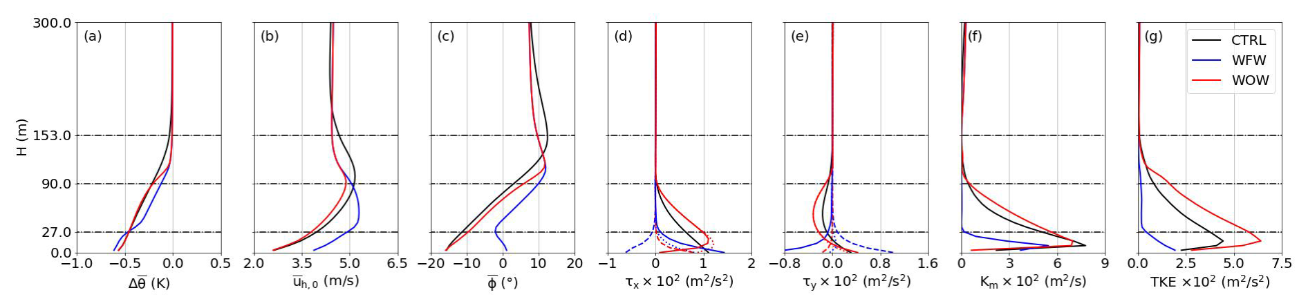
Figure 6 Vertical profiles of temporally (1 h) and horizontally averaged potential temperature (a), wind speed (b), wind direction relative to the x axis (c), stresses (dotted line, dashed line, and solid line represent turbulent stress, wave-induced stress, and total stress, respectively) (d, e), momentum eddy diffusivity (f), and turbulent kinetic energy (g) from the precursor simulations. The black line represents the control case without wave effects, and the blue and red lines denote the cases with wind-following and wind-opposing waves, respectively. The dash-dotted lines mark the wind turbine rotor's bottom, center, and top.

The observed variations in wind profiles are directly attributed to the wave-induced modification of stresses near the ocean surface. As depicted in Fig. 6d and e, waves generate stresses that align with their direction of propagation. In the WFW case, the wave field neutralizes over 80 % of the turbulent stress in the x direction and introduces a positive stress in the y direction. This is the main cause of the increased wind speed and the northerly shift in wind direction. Similar results were also observed in phase-resolved LESs by Sullivan et al. (2008). Conversely, in the WOW case, surface stresses are enhanced due to the opposing waves. These wave effects also manifest in the turbulent characteristics of the airflow. Changes in wind shear alter the parameterized momentum eddy diffusivity K_m, subsequently affecting turbulence quantities. Figure 6f and g show that in the WFW scenario, K_m is reduced to nearly zero at the rotor's bottom height, and the turbulence almost disappears beyond this height. In contrast, the WOW scenario shows a significant increase in TKE throughout the boundary layer.

To sum up, the presence of swells directly influences the momentum exchange at the wind–wave interface and, consequently, the magnitude and direction of surface stresses. This leads to a remarkable modification of the wind shear and veer close to the waves. Although wave-induced stresses reduce significantly, by approximately 96 % at a height of half the wave's wavelength according to Eq. (8), these near-surface variations are further extended upwards beyond the operational height of the wind farm. This upward spread occurs through turbulent mixing as a new equilibrium is established within the entire Ekman layer, highlighting the profound influence of swells on wind farm aerodynamics.

3.2 Wind farm

3.2.1 Flow field

Figure 7 illustrates the 1 h averaged flow field quantities, including wind speed, wind direction, and turbulence intensity for the WFW-C12 case (left column) and its differences from the control case WFW-CTRL (right column) at the hub height horizontal plane. The turbulence intensity is defined as

$$\begin{array}{}\text{(14)}& \text{TI}={\displaystyle \frac{\sqrt{\frac{\mathrm{1}}{\mathrm{3}}(\stackrel{\mathrm{‾}}{u^{\prime }{u}^{\prime }}+\stackrel{\mathrm{‾}}{v^{\prime }{v}^{\prime }}+\stackrel{\mathrm{‾}}{w^{\prime }{w}^{\prime }})}}{{\stackrel{\mathrm{‾}}{u}}_{\mathrm{h},\mathrm{0}}}},\end{array}$$

where ${\stackrel{\mathrm{‾}}{u}}_{\mathrm{h},\mathrm{0}}$ is the inflow velocity. The wake region behind the wind farm is distinctly characterized by the reduced wind speed, change in wind direction, and significantly enhanced turbulence intensity. As observed in Fig. 7c and through streamlines, the wind within the wake zone undergoes a gradual counterclockwise rotation, leading to a directional shift of approximately −10° at the domain's outlet. This phenomenon of wake deflection is attributed to the decrease in Coriolis force (which is proportional to wind speed) in the wake and is typically observed in large-scale wind farms, as noted by Maas and Raasch (2022).

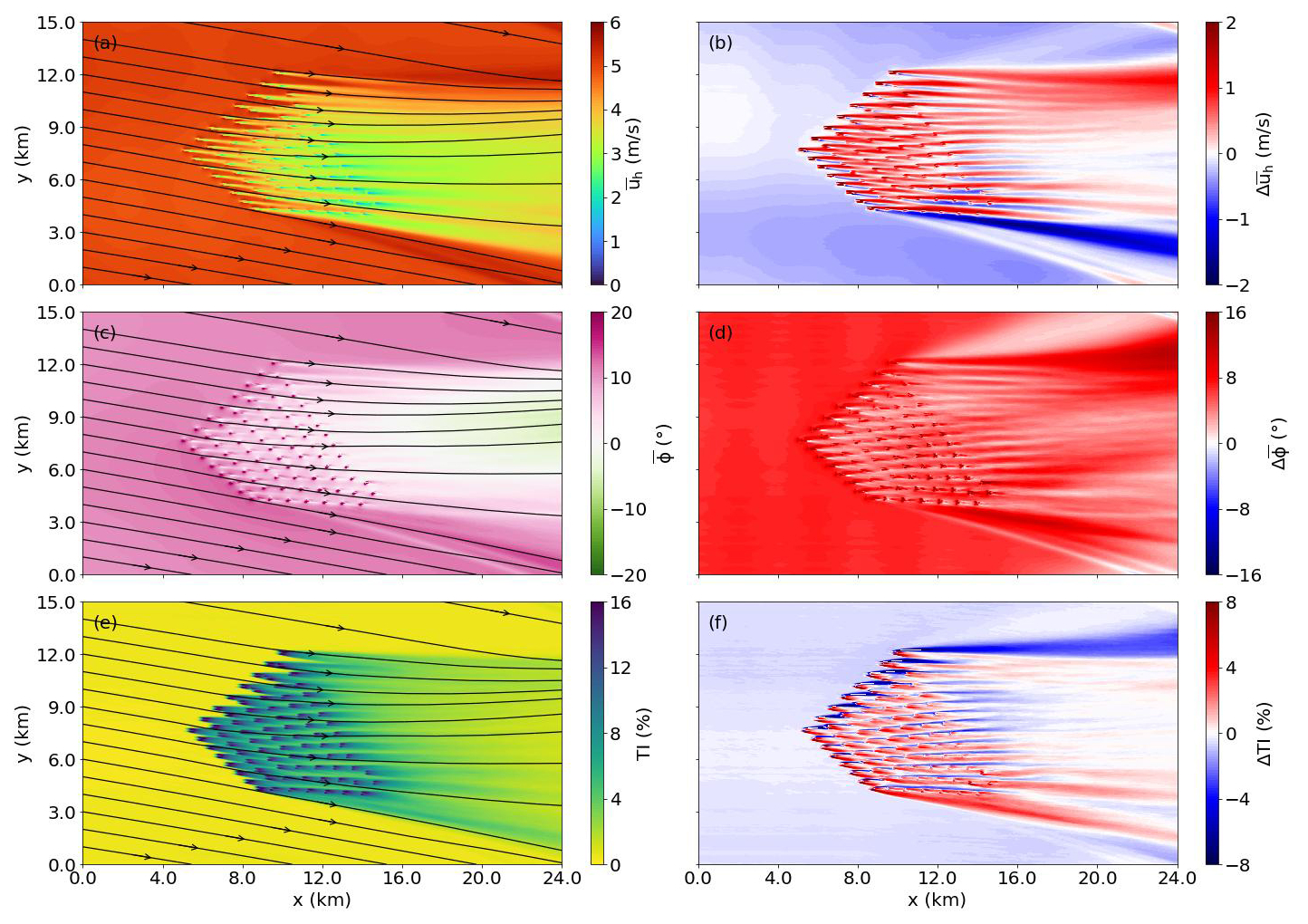
Figure 7 Mean wind speed (a), mean wind direction (c), and turbulence intensity (e) at the hub height horizontal plane for the WFW-C12 case. Subplots in the right column (b, d, f) are differences in corresponding quantities between the WFW-C12 case and its control case WFW-CTRL. The solid black lines with arrows are streamlines.

In comparison to the WFW-CTRL case, introducing waves in the WFW-C12 case results in a slight decrease in inflow wind speed at hub height. Immediately downstream of each wind turbine, there is an acceleration of wind speed, while the waves do not significantly impact the wind speed in the farther wake region. A notable effect caused by wind-following waves is the clockwise rotation (positive $\mathrm{\Delta }\stackrel{\mathrm{‾}}{\mathit{\varphi }}$) of the wind in both the inflow and the wake flow. As explained in Sect. 3.1, this is because the wave-induced stress alters the original Ekman equilibrium among the pressure gradient, turbulent stress, and Coriolis force, and the wind direction has to shift to reach a new balance. Furthermore, the turbulence intensity of the inflow shows a reduction relative to the case without wave influence, as wave-induced stress partially offsets the surface friction. However, the TI in the wake region remains largely unchanged, regardless of the presence or absence of waves.

Figure 8 presents the same flow field information as Fig. 7 but for WOW-C10 and its differences from WOW-CTRL. In WOW-C10, the presence of wind-opposing waves leads to a reduction in inflow wind speed and a slight clockwise directional shift, consistent with observations in Fig. 6b and c. While the near-wake flow speed in the WOW-C10 case is marginally lower than in WOW-CTRL, the far-wake region appears relatively unaffected by waves. However, the shift in wind direction is pronounced: the wake flow exhibits a notable counterclockwise rotation (negative $\mathrm{\Delta }\stackrel{\mathrm{‾}}{\mathit{\varphi }}$), as marked by the blue region in Fig. 8d. Despite the wind-opposing waves enhancing momentum exchange and turbulence in the inflow, the turbulence intensity at hub height within both the near- and far-wake regions remains at the same level as that in the control case.

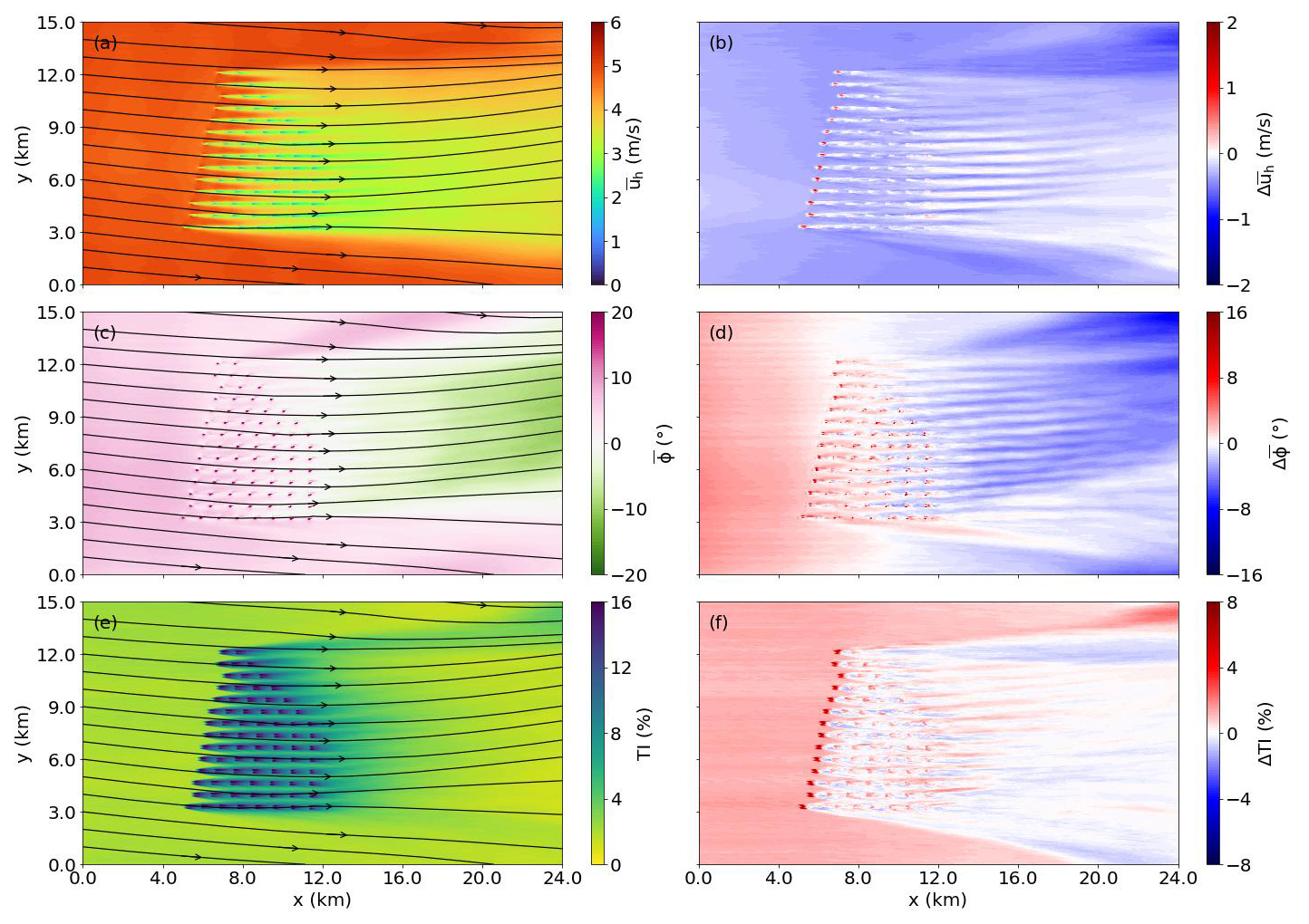
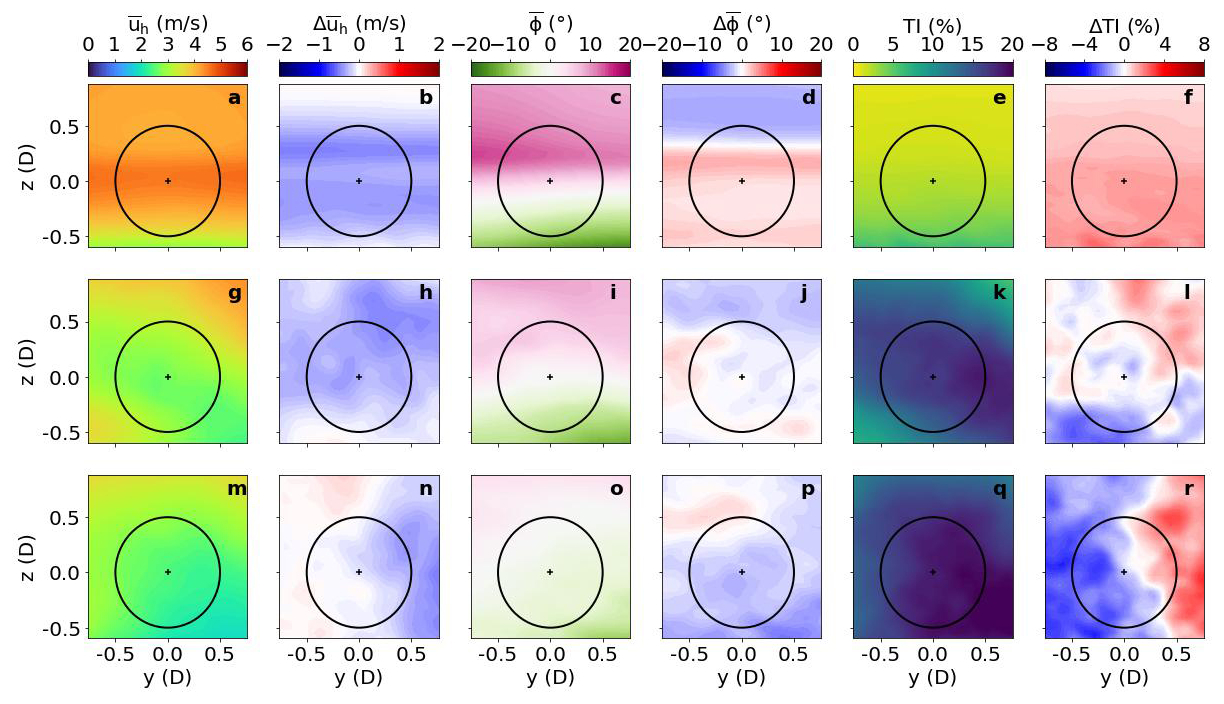
Figure 8 Same as in Fig. 7 but for the WOW-C10 case and the differences from the WOW-CTRL case.

To analyze the wake flow and highlight the differences between cases with and without wave effects, we defined the wake region as areas where the velocity deficit exceeds 0.05. The velocity deficit is calculated as the relative reduction in velocity from the inflow, expressed as $\mathrm{1.0}-u_{\mathrm{h}}/u_{\mathrm{h},\mathrm{0}}$, where u_h is the velocity at the hub height within the wake, and u_h,0 is the inflow velocity at the same height. Downstream along the x axis, we computed the wake width by measuring the span between its left and right wake edges. Additionally, we evaluated the velocity deficit, wind direction, and turbulence intensity, averaged across the wake width at each x position. This enables a detailed examination of how waves impact wake development. These wake statistics along the x axis for all cases are illustrated in Fig. 9.

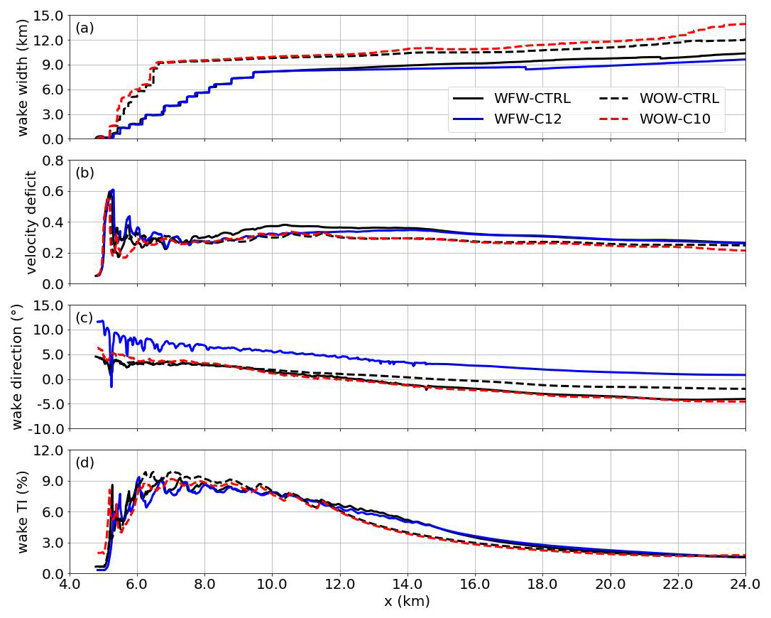
Figure 9 Evolution of the wake statistics along the x axis: wake width (a), velocity deficit (b), wake direction (c), wake turbulence intensity (d). The WFW-CTRL, WOW-CTRL, WFW-C12, and WOW-C10 cases are represented by the solid black line, solid blue line, dashed black line, and dashed red line, respectively.

Figure 9a indicates that within the wind farm, the wake width remains unaffected by wave conditions. However, further downstream, the wake width is influenced depending on the wave direction: it is narrowed by wind-following waves and broadened by wind-opposing waves. This variation in wake width due to wave influence extends from a few hundred meters just behind the wind farm to approximately 2.0 km near the domain's outlet. Regarding velocity deficit, simulations with and without wave effects show almost consistent results for different wave directions, with only minor fluctuations observed within the wind farm. In contrast, the impact of waves on wind direction is more significant. In the WFW-C12 case, the wake direction shifts by over 5° compared to WFW-CTRL, while in WOW-C10, the shift is about −3° relative to WOW-CTRL. A directional shift of 3–5° implies a crosswise wake deviation of approximately 50.0 to 120.0 m at a normal streamwise spacing in a wind farm, which could lead to a strong impact on the total wind farm power output. Furthermore, the turbulence intensity at hub height appears to be minimally influenced by wave conditions in both scenarios. Across all cases, TI exhibits a consistent trend in the streamwise direction: it increases sharply at the front part of the wind farm; slightly decreases until the last row of wind turbines; and finally slowly reverts to the ambient level in the distant wake region, typically beyond the extent of one wind farm length. Though the entire wake flow is not available due to limitation in domain size, the convergence of velocity deficit and turbulence intensity levels across different cases at the downstream boundary suggests that the wake recovery process, and consequently the wake length, in a stable boundary layer with low wind speed is not significantly affected by the presence of swell.

Figures 10 and 11 present the time-averaged flow statistics on the x–z plane through the wind farm's center. In both the WFW-C12 and WOW-C10 cases, an internal boundary layer (IBL) begins to form immediately behind the first row of turbines. In contrast to the growth pattern seen in conventionally neutral boundary layers (CNBLs), where the IBL's vertical extent can reach heights of 3D to 4D downwind (Allaerts and Meyers, 2017), our scenarios show a different behavior. In our simulations, the cold air at the lower part of the boundary layer is entrained and drawn upward under the mixing effect of the wake turbulence, forming a sharper temperature gradient at the top of the IBL. This in turn restrains further expansion of the IBL, which ceases its growth at approximately 2D height, indicated by the dashed black lines.

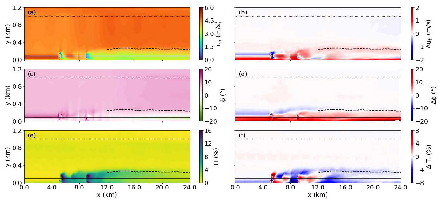
Figure 10 Mean wind speed (a), mean wind direction (c), and turbulence intensity (e) at the central x–z plane for the WFW-C12 case. Subplots in the right column (b, d, f) are differences in corresponding quantities between the WFW-C12 case and its control case WFW-CTRL. The solid black line and the dotted line are the hub height and the bottom of the inversion layer. The dashed line marks the top of the internal boundary layer.

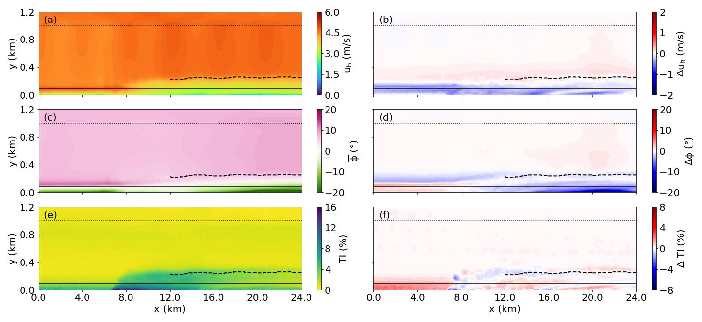
Figure 11 Same as in Fig. 10 but for the WOW-C1 case and the differences from the WOW-CTRL case.

The heights of the IBL in the control cases along the x direction align closely with those in the wave-affected scenarios, indicating that the evolution of the upper part of wake flow is hardly affected by wave conditions. However, the effects of waves on the flow below the hub height are notably distinctive. In Fig. 10b and d, it is observed that, in the WFW-C12 case, the wind speed near the surface can exceed that of WFW-CTRL by 1.0 to 1.5 m s⁻¹. Additionally, a significant clockwise rotation in wind direction is evident in the dark-red region below the hub height line. Wave effects are also apparent in the comparison between the WOW-CTRL and WOW-C10 cases, as shown in Fig. 11. Here, under the influence of wind-opposing waves, there is a noticeable decrease in velocity below hub height, accompanied by a counterclockwise shift in wind direction. The impact of waves on the turbulence intensity within the wind farm wake flow in our study is less pronounced, in contrast to the enhanced TI and faster wake recovery of a single wind turbine under wind-opposing wave conditions reported by Yang et al. (2022b). This is mainly because the wake's turbulence is predominantly mechanical turbulence originating from the wind turbines themselves, which overwhelms the wave-induced turbulence.

3.2.2 Energy budget analysis

The integration of each term in the energy budget was computed over the control volume of the wind farm, denoted as Ω_wf. This volume extends horizontally to 3D beyond the wind farm's edges, as outlined by the black squares in Fig. 4. Vertically, Ω_wf spans from 15 to 201 m above the surface. The results are presented in Fig. 12. Theoretically, in an equilibrium state, the mean kinetic energy of a flow field should remain constant, implying that the sum of the terms on the right-hand side of Eq. (13) would be zero. However, in our simulations, this sum yields a positive value. This discrepancy can be attributed to two primary reasons: firstly, the flow never reaches a perfectly steady state due to the continuous evolution of the potential temperature profile (as shown in Fig. 6a) driven by the imposed surface cooling setup (Sanchez Gomez et al., 2023). Secondly, there is an inherent underestimation of dissipation resulting from the numerical integration method and the computational schemes used in the PALM code, as discussed in Maas (2023a). To account for this, we combine this residual with the dissipation term, treating them as a single energy sink term, denoted as 𝒟+ℛ.

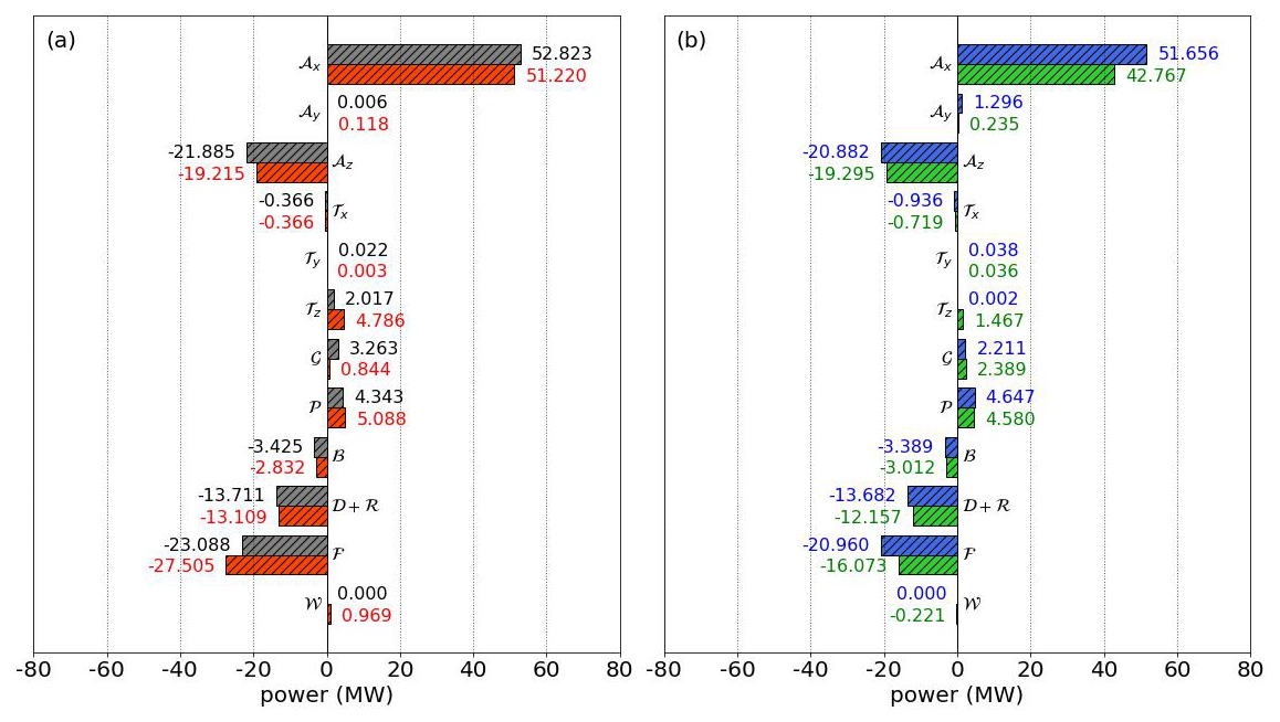
Figure 12 The mean kinetic energy budget terms in the wind farm control volume for WFW-CTRL and WFW-C12 (a) and WOW-CTRL and WOW-C1 (b). WFW-CTRL, WFW-C12, WOW-CTRL, and WOW-C1 are colored gray, red, blue, and green, respectively.

We find that the inclusion of swell does not qualitatively alter the energy source and sink terms. In all four cases in this study, six common terms contribute to the total energy input: 𝒜_x, 𝒜_y, 𝒯_y, 𝒯_z, 𝒢, and 𝒫. Among them, the advection of kinetic energy in the x direction 𝒜_x is the predominant source of energy. Notably, the kinetic energy transport in the y direction by both the mean flow (𝒜_y) and turbulence (𝒯_y) is significantly less, typically 2 to 3 orders of magnitude smaller than 𝒜_x. Compared to the findings in Maas (2023b), where the vertical turbulent transport of ${\stackrel{\mathrm{‾}}{E}}_k$, i.e., 𝒯_z, is comparable to 𝒜_x, our simulations under stable atmospheric conditions exhibit different behavior. In our cases, the turbulence is suppressed by the buoyancy force, and the wake turbulence intensity rapidly reverts to the ambient level. As a result, the vertical turbulent transport term, 𝒯_z, is an order of magnitude smaller than 𝒜_x, leading to a slow recovery of velocity deficit (as also shown in Fig. 9). The common energy sink in all cases includes the vertical transport by mean flow 𝒜_z, turbulent transport along the x axis 𝒯_x (which is negligible), the buoyancy term ℬ, dissipation 𝒟+ℛ, and energy extraction by the wind farm ℱ. It is worth noting that while the buoyancy term ℬ is relatively small in magnitude in all simulations, it can be a significant factor in strongly stable or convective stability conditions.

Compared to the WFW-CTRL case, the magnitudes of 𝒜_x and 𝒜_z in the WFW-C12 case exhibit slight reductions of 3.0 % and 12.2 %, respectively. This is primarily attributed to changes in the mean wind speed profile influenced by wind-following swell effects. Additionally, despite a notable reduction in turbulence at the lower boundary of Ω_wf in WFW-C12, there is a substantial increase of 137.3 % in 𝒯_z. This increase is caused by the combination of an upward turbulent momentum flux (negative turbulent stress) and a negative wind shear induced by waves. A sharp decrease in the geostrophic term 𝒢 is mainly due to the clockwise shift in the wind direction, resulting in a negative $\stackrel{\mathrm{‾}}{v}$. Notably, the contribution to ${\stackrel{\mathrm{‾}}{E}}_k$ from the wave-induced stresses itself is relatively minor, only constituting about 1.5 % of the total energy input. However, it leads to a 19.1 % increase in energy extraction by the wind farm. This implies that the impact of waves on the wind farm's energy budget is primarily indirect, through modifications to the mean wind speed and direction, rather than from the wave-induced stresses themselves. Variations in other terms are of a magnitude of 0.1 MW for 80 wind turbines in total and thus are considered insensitive to the presence of swells.

In the WOW-C1 case, the presence of wind-opposing waves results in a reduction in wind speed at various levels throughout the rotor range, leading to a decrease of 17.2 % in 𝒜_x and 7.6 % in 𝒜_z compared to the WOW-CTRL case. 𝒯_z shows a remarkable increase, but unlike in the WFW-C12 case, this increase is due to the enhanced kinetic energy entrainment across the upper Ω_wf boundary. The geostrophic term 𝒢 remains largely unchanged, as the wind direction is not significantly affected by the opposing waves. The energy sink related to τ_w is minimal, at only −0.2 MW (0.4 % of the total sink). However, the indirect effects of the waves lead to a substantial 23.3 % reduction in energy extraction by the wind farm.

Figure 13 shows the power density profiles of budget terms (except for those in the y dimension). The integration of these profiles along the z axis gives the corresponding budget values as in Fig. 12. It provides a clear view of the wave effects on the ${\stackrel{\mathrm{‾}}{E}}_k$ budget terms at various height levels. Figure 13a illustrates highly consistent profile shapes of 𝒜_x and wind speed (see also Fig. 6b), indicating again that 𝒜_x is largely determined by the inflow wind profile. Due to the presence of a velocity deficit in the wake, the inflow at the x axis boundaries of Ω_wf exceeds the outflow, causing the mean flow to diverge through the top and bottom planes. Consequently, any acceleration of wind speed at these boundaries results in a greater amount of kinetic energy being carried away, and vice versa. This is the reason for the larger magnitude of 𝒜_z near the surface and a smaller one at the rotor top in WFW-C12 compared to WFW-CTRL. The wind-following wave condition in WFW-C12 induces negative wind shear and alters the direction of turbulent momentum flux, accounting for the increased 𝒯_z across the rotor, while the larger 𝒯_z in WOW-C1 compared to WOW-CTRL is mainly observed at the upper part of the rotor. Figure 13d demonstrates the influence of wind direction on the geostrophic term 𝒢. A clockwise shift in wind leads to a reduction in 𝒢. As for the energy contributions from mean perturbation pressure 𝒫 and the energy sinks due to buoyancy ℬ and dissipation 𝒟+ℛ, these terms are not sensitive to the presence of waves in both the WFW-C12 and WOW-C1 cases, even near the surface. Figure 13i displays the exponential decay of ${\stackrel{\mathrm{‾}}{E}}_k$ rate of change directly caused by the wave-induced stresses, which die out quickly above the height of $z=-\mathrm{0.5}$D.

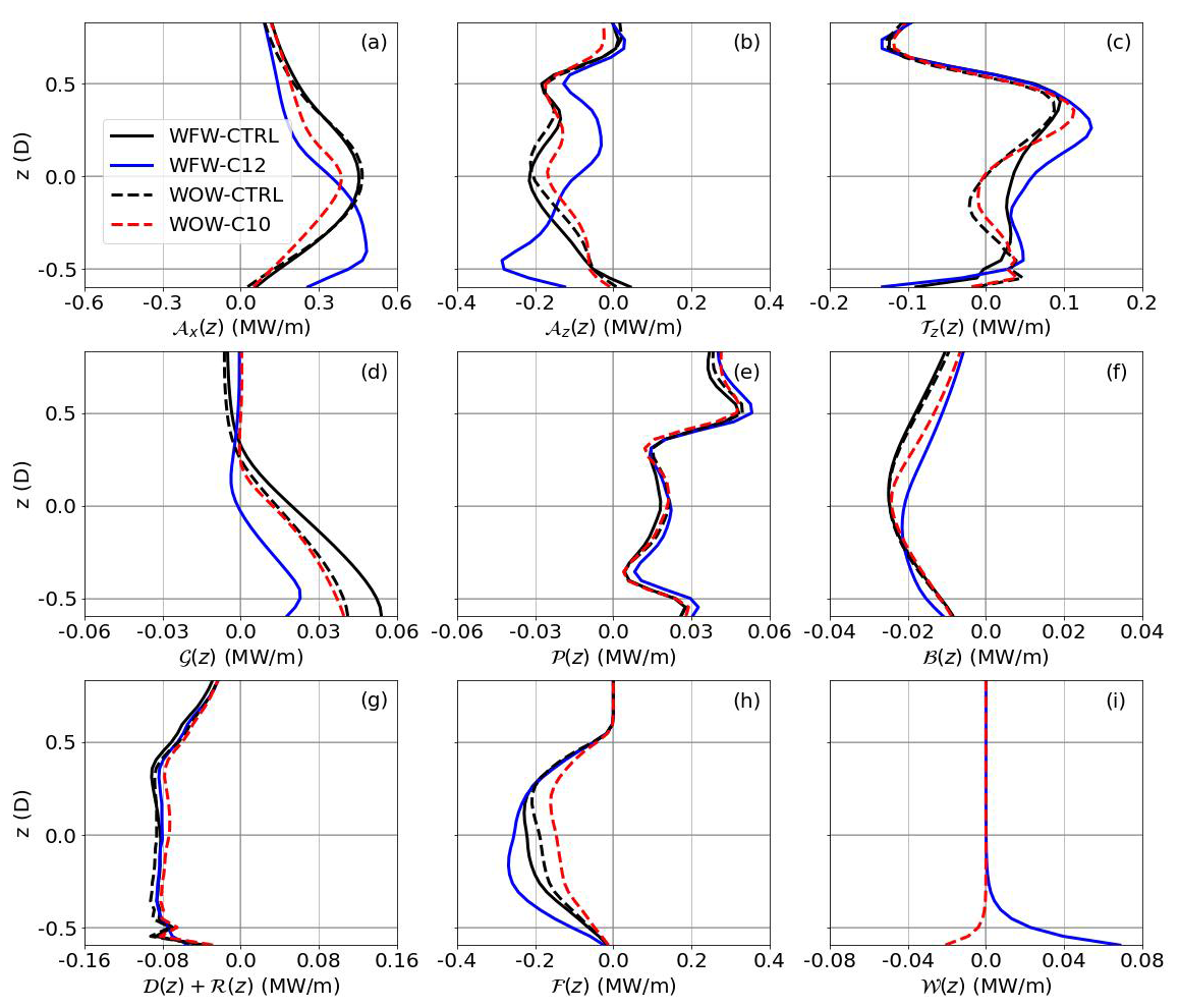
Figure 13 The power density vertical profiles of each mean kinetic energy budget term for WFW-CTRL (solid black), WFW-C12 (solid blue), WOW-CTRL (dashed black), and WOW-C1 (dashed red).

3.3 Wind turbine

3.3.1 Flow field

While the previous section addressed the impact of waves on the overall wind farm, this section explores the variation in wave effects among individual wind turbines at different positions, intending to provide a clearer picture of the wave-influenced airflow dynamics inside the wind farm. To achieve this, we chose three representative turbines in each case (marked by cross signs in Fig. 4): turbine nos. 80, 54, and 1 for the WFW-CTRL and WFW-C12 cases and turbine nos. 73, 41, and 28 for the WOW-CTRL and WOW-C1 cases. These turbines are selected to represent the front (WT-F), middle (WT-M), and back (WT-B) segments, offering a comprehensive view of the wave effects across the entire wind farm.

Figure 14 plots the mean horizontal wind speed (column 1), wind direction (column 3), and turbulence intensity (column 5) for the wind turbines at the front (row 1), middle (row 2), and back parts (row 3) of the wind farm in the WFW-C12 case, and the corresponding differences between the WFW-C12 and WFW-CTRL cases are shown in columns 2, 4, and 6. WT-F reflects the conditions experienced by the first-row turbines, which are subject to swell impacts similar to those on the ambient inflow, as shown in Fig. 6. The wind speed's acceleration and the clockwise shift in wind direction at the lower rotor section, due to wind-following waves, are evident in Fig. 14b and d, where TI is also observed to be slightly lower near the surface. WT-M benefits from this altered wind direction and remains unobstructed by upstream wake flow. Consequently, there's a notable increase in wind speed and a reduction in TI throughout the rotor area compared to the corresponding turbine in the WFW-CTRL case. WT-B's rotor is partially covered by wake, resulting in higher wind speeds and reduced turbulence on the right half of the rotor compared to the left. Notably, the influence of waves on airflow inside the wind farm progressively extends from the lower rotor area in the front row to higher altitudes in the middle, eventually impacting the entire rotor area in the farm's rear region.

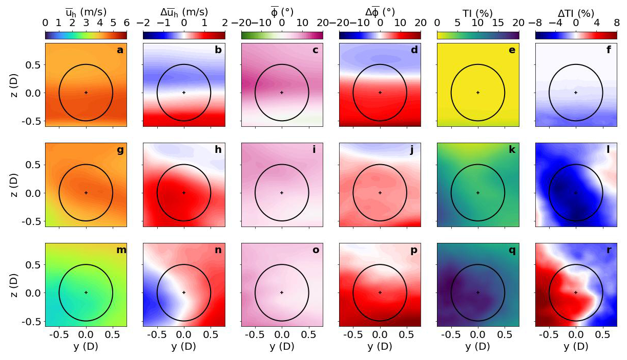
Figure 14 Flow statistics in the rotor planes of three wind turbines at the front, middle, and back positions in the wind farm for the WFW-C12 case and the differences between WFW-C12 and WFW-CTRL. Columns 1, 3, and 5 show the mean horizontal wind speed, wind direction, and turbulence intensity, respectively. Columns 2, 4, and 6 are the differences in the corresponding quantities from the WFW-CTRL case.

The most pronounced influence of wind-opposing waves is the intensification of turbulence. In the WOW-C1 case, WT-F encounters stronger turbulence across the entire rotor compared to its counterpart in WOW-CTRL, as seen in Fig. 15f. The wind speed is slightly reduced, while the wind direction is barely changed, contrasting with conditions under wind-following waves. The wave-induced variations in flow quantities gradually decay further downstream. The inflow direction and TI for WT-M in WOW-C1 are almost consistent with those in WOW-CTRL, although the decrease in velocity is still present. WT-B in the last row faces an asymmetric inflow turbulence due to its yaw adjustment to the south.

Figure 15 Same as in Fig. 14 but for the WOW-C1 case and the differences from the WOW-CTRL case.

3.3.2 Energy budget analysis

With the same analysis method as discussed in Sect. 3.2.2, but focusing on the individual wind turbine control volume Ω_wt as shown by gray squares in Fig. 4, we calculate the mean kinetic energy budget terms for three selected turbines in each simulation case and demonstrate the results in Fig. 16.

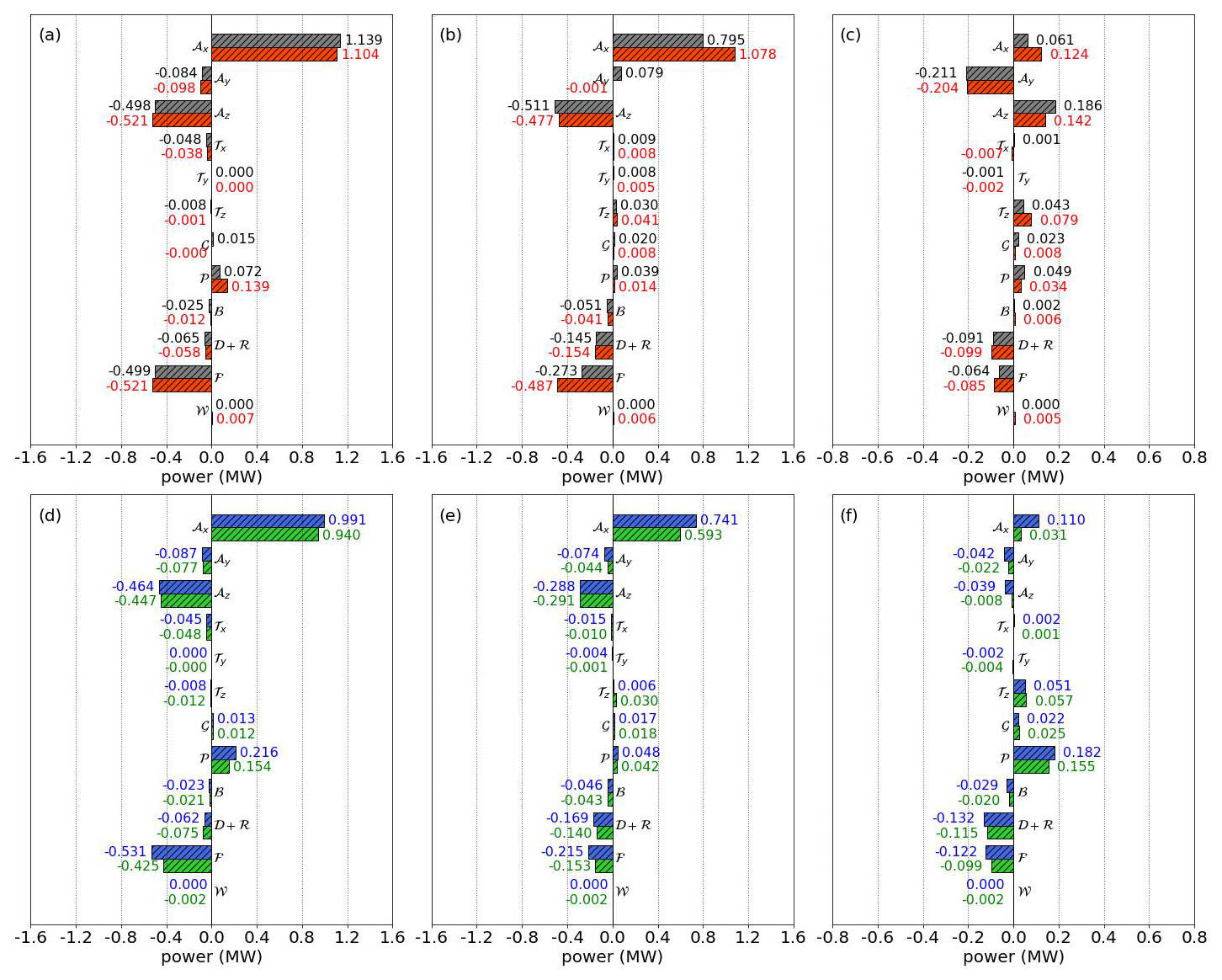
Figure 16 The mean kinetic energy budget terms in the wind turbine control volumes for WFW-CTRL and WFW-C12 (a–c) and WOW-CTRL and WOW-C1 (d–f). WFW-CTRL, WFW-C12, WOW-CTRL, and WOW-C1 are colored gray, red, blue, and green. The left, middle, and right columns represent the front, middle, and back wind turbine positions in the wind farm.

As a result of the accumulating velocity deficit in wake flow, the primary energy source 𝒜_x for a wind turbine's control volume diminishes progressively downstream, with 𝒜_x of WT-B being merely about 10.0 % of that of WT-F. This aligns with findings from previous LES studies by Allaerts and Meyers (2017) and Maas (2023b). 𝒜_y is mainly attributed to the asymmetry of the inflow. For front-row turbines, 𝒜_y arises from yaw misalignment, while for turbines further back, it is mainly influenced by rotor wake interference. For instance, WT-B in the WFW-CTRL and WFW-C12 cases experiences partial wake obstruction, leading to a significant disparity in velocities at its left and right sides. This results in a substantially higher 𝒜_y for WT-B. To compensate for the KE loss through lateral boundaries, there's a corresponding increase in 𝒜_z, contrasting with the conditions experienced by WT-F and WT-M, where such wake obstruction is less pronounced or absent (column 2 in Fig. 14). The influence of waves on the kinetic energy advection along the x axis, 𝒜_x, becomes increasingly pronounced for wind turbines located further downstream. In the WFW-C12 case, which involves wind-following waves, the changes in 𝒜_x compared to WFW-CTRL are −3.1 % for WT-F, 35.6 % for WT-M, and 103.3 % for WT-B. The corresponding differences due to wind-opposing wave conditions between WOW-C1 and WOW-CTRL are −5.1 %, −20.0 %, and −71.8 %, respectively.

The turbulent transport of ${\stackrel{\mathrm{‾}}{E}}_k$ is marginal in magnitude compared with the contribution from advection. However, it is worth noting that the waves result in a remarkable increase (83.7 %) in 𝒯_z for the last-row turbine in WFW-C12, while this increase in WOW-C1 is only 11.8 %. As for the geostrophic term 𝒢, there is a consistent trend of increase downstream in both cases. However, 𝒢 is largely reduced in WFW-C12 due to the presence of waves. 𝒫 signifies the work performed by perturbation pressure across the wind turbine control volume Ω_wt. It is elevated at both the front and rear of the wind farm. This increase is due to the larger pressure gradients present at these boundaries. In the presence of wind-following waves, 𝒫 increases at the front row, as these waves intensify the pressure drop in the x direction across the rotor. Conversely, wind-opposing waves reduce 𝒫 by decreasing this pressure drop. The velocity changes induced by waves have a relatively minor effect on variations in 𝒫. Downstream, 𝒫 exhibits non-monotonic variations, potentially linked to the small-scale gravity wave oscillations identified in the study by Maas (2023b). The dissipation term 𝒟+ℛ, as expected, follows the variation trend of turbulence intensity, exhibiting a greater magnitude within the wind farm than at its edges. Interestingly, though the change in the absolute magnitude of the energy extraction term ℱ due to waves decreases downstream, the relative change is more pronounced for WT-M compared to WT-F and WT-B.

3.3.3 Yaw and power extraction

In practice, wind turbines work with a control system designed to optimize power output by adjusting their operational states. Yawing control is a critical part of this system because the wake direction is largely determined by the yaw angle, and the total energy production could vary by a wide range with different yawing conditions given the same wind farm layout (Bastankhah and Porté-Agel, 2019; Munters and Meyers, 2018). The yawing control module in PALM is turned on in the present study so that each wind turbine adjusts its yaw angle according to the local wind direction until the yaw misalignment threshold of 5.0° is reached, and the yawing speed is set to 0.3° s⁻¹.

Figure 17 gives a comprehensive view of how swells from two opposite directions affect the yawing behavior of wind turbines at various positions within the wind farm, and Table 2 details the yaw statistics for all four cases. In the WFW-C12 case, the first-row turbines yaw northwards to align with the clockwise-shifted wind under the wind-following swell effects, with an average yaw angle difference of about 10° compared to WFW-CTRL. This variation rapidly phases out for turbines deeper within the wind farm, as indicated by the gradual fading of the rose color from west to east in Fig. 17a. However, turbines in the rear section (no. 1 to no. 22) exhibit larger yaw angle differences again. These discrepancies are mainly due to the wave influences on the wind farm wake deflection. The increase in wind speed below the hub height, caused by wind-following waves, mitigates the wake's velocity deficit, thereby reducing the geostrophic force responsible for wake deflection. This phenomenon becomes more evident in the downstream turbines. The pattern where yaw differences are more pronounced at the front and back of the wind farm than in the middle is also observed between WOW-C1 and WOW-CTRL (as shown in Fig. 17), though with a smaller magnitude of the average yaw difference Δγ. The wind-opposing waves aggravate the velocity deficit across the wind farm, causing the wake flow to veer further leftward. Consequently, turbines at the back rows rotate towards the south to minimize yaw misalignment.

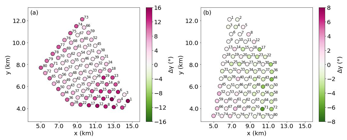
Figure 17 The yaw angle difference in each wind turbine between WFW-C12 and WFW-CTRL (a) and between WOW-C1 and WOW-CTRL (b).

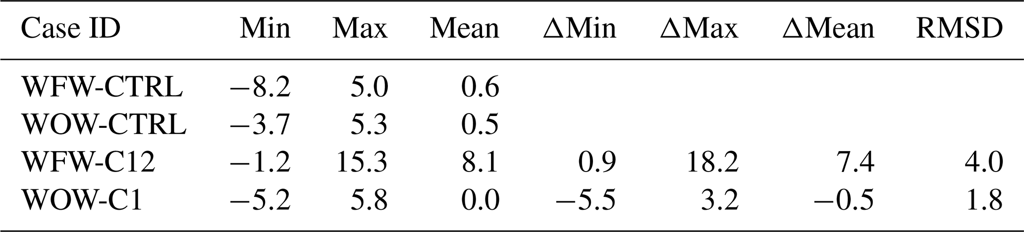
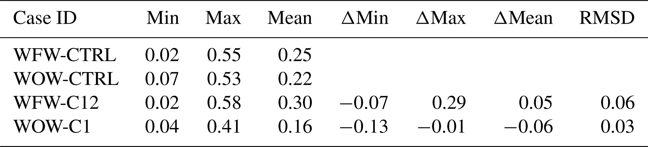
Table 2 Wind turbine yaw angle statistics in degrees. Δ signifies the difference from the corresponding control case. RMSD is the root mean square deviation.

The differences in energy production caused by waves are illustrated in Fig. 18, and Table 3 lists the related statistics. It is worth noting that while the first-row wind turbines in WFW-C12 gain more energy than those in WFW-CTRL due to the larger inflow wind speed, the maximal power increase appears in the middle region, where the turbines are less influenced by the upwind wake flow as a result of wind shifting. The powers of turbines in the rear region are slightly increased, except for no. 3 and no. 4, which are fully covered by the shifted wake. The total energy extraction increases from 20.0 to 24.0 MW, i.e., an improvement of 20.0 %, which is considered a substantial value for a large-scale wind farm. By contrast, when swells propagate against the wind, they result in a power reduction for each wind turbine, and this reduction value decreases from approximately −0.1 MW in the front row to −0.01 MW in the last row. The overall energy extraction loss in WOW-C1 due to waves is 4.8 MW (−27.3 %), with the maximal individual difference reaching −0.13 MW.

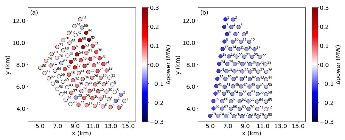
Figure 18 The power extraction difference in each wind turbine between WFW-C12 and WFW-CTRL (a) and between WOW-C1 and WOW-CTRL (b).

Table 3 Wind turbine power extraction statistics in MW. Δ signifies the difference from the corresponding control case. RMSD is the root mean square deviation.

4 Discussion and conclusions

The interaction between the atmosphere and ocean waves, especially swells, has gained considerable research interest for their strong influence on the dynamics of marine atmospheric boundary layer flows and the operation of large-scale wind farms. Nevertheless, most prior numerical studies have been limited to neutral stability conditions and idealized wind farm layouts. To address this gap, the present large-eddy simulation study focuses on an actual wind farm situated at the North Sea and investigates the swell impacts on both wind farm performance and wake flow dynamics under stably stratified boundary layer flows.

We enhance the original wall-stress model in PALM to capture the effects of waves accurately with a new parameterization method. This method computes the vertical profiles of wave-induced stresses using a predefined wave spectrum, enabling it to simulate more complex wind–wave interaction scenarios. Specifically, it effectively represents upward momentum fluxes and cases involving misalignment between wind and wave directions. Based on the wind and wave data from May 2015 to April 2016, we identify two representative scenarios characterized by moderate wind speeds (5.0 m s⁻¹) and fast wave (12.0 and 10.0 m s⁻¹) conditions: the first involves a northwesterly wind accompanied by a wind-following wave, with a slight misalignment angle of 22.5°; the second includes an easterly wind opposed by a westerly originated wave. We are interested in the wave impacts under stable conditions because in such cases the wind turbulence is suppressed, and thus the wave-induced momentum plays a more important role in the boundary layer flows (Jiang, 2020).

In both selected scenarios, the presence of waves significantly influences the inflow characteristics. For the wind-following wave case, the waves induce an ageostrophic jet below the hub height, along with a clockwise wind shift and a notable reduction in turbulence intensity. In contrast, the wind-opposing wave scenario leads to reduced wind speeds and increased turbulence intensity across the rotor, with minimal change in inflow direction. These effects are quantitatively consistent with the results of previous numerical studies conducted under neutral conditions (Sullivan et al., 2008; Jiang et al., 2016). A key distinction in wind–wave interaction under neutral versus stable conditions is the height of the stable boundary layer, which in our simulations is about 160.0 m, significantly less than the typical 1.0 km height of a neutral boundary layer. This results in more pronounced wave-induced wind shear, wind veer, and turbulence intensity variations exactly within the operational height range of a wind farm. This underscores the research significance of these scenarios in the context of wind farm operations.

Partly aligned with the simulation results from Yang et al. (2022b, a), the differences in wind speed and turbulence intensity due to waves are detected inside the wind farm. Compared to the case without waves, a weaker TI and thus slower recovery of velocity deficit is found in the WFW case. However, for the WOW case, there is neither a strong enhancement of TI in the wake flow nor a remarkable faster recovery. There are two main reasons: firstly, the wave heights used in this study (1.36 m for WFW and 0.96 m for WOW) are smaller than theirs (3.2 m); secondly, the wind farm in our case is much larger (80 turbines) compared to the wind turbine arrays in their study (6 turbines). As a result, the extra TI in the inflow induced by waves is rapidly overwhelmed by the mechanical turbulence generated by the wind turbines. Furthermore, the influence of waves on the wind speed and TI of the wind farm's wake flow diminishes rapidly as it moves downstream and is barely distinguishable in the far-wake region (Fig. 9). Nevertheless, waves can significantly change the flow direction by inducing a crosswise velocity component and modifying the Coriolis force within the wake. This wind direction shift persists until the domain's end and notably influences the aerodynamic performance of downstream wind turbines.

The analysis of kinetic energy budget terms over wind farm control volume Ω_wf reveals that waves influence the ${\stackrel{\mathrm{‾}}{E}}_k$ balance mainly by increasing (WFW)/decreasing (WOW) mean wind speed and thus modifying the energy advection in the x and z directions, i.e., 𝒜_x and 𝒜_z. Furthermore, the vertical turbulent transport term 𝒯_z is also substantially affected. 𝒯_z in the WFW case increases due to the wave-induced upward momentum fluxes and the negative wind shear, while the increase in 𝒯_z in the WOW case is a result of the enhanced turbulence at the top of Ω_wf. However, the direct wave-induced energy term 𝒲 is negligibly small, accounting for only 1.5 % and 0.4 % of the total power in both cases.

In addition, the aerodynamics of three wind turbines representative of the front, middle, and back regions of the wind farm are also analyzed to investigate how the wave influences vary with position in the wind farm. ${\stackrel{\mathrm{‾}}{E}}_k$ budget term analysis over Ω_wt shows that, though the absolute wave-induced wind decays quickly, the relative changes in energy advection for individual turbines increase downstream; e.g., the changes in 𝒜_x are 3.1 % and −5.1 % for WT-F, 35.6 % and −20.0 % for WT-M, and 103.3 % and −71.8 % for WT-B in the WFW and WOW cases, respectively.

While waves mainly impact the energy harvesting of wind turbines through changes in energy advection, the role of wind direction shift and corresponding yaw adjustments plays a crucial role in this process. In the wind-following wave scenario, the most substantial power changes occur in the middle section of the wind farm. This is primarily because the reduction in inflow wind caused by upstream wake effects is significantly mitigated for these turbines due to the wave presence. The alteration in energy production related to wind shift depends highly upon the ambient wind direction and the specific layout of the wind farm. Previous research has not paid enough attention to this aspect. Incorporating yawing control is therefore critical and should be a key consideration in future studies on this topic.

In brief, the main contributions and findings of the present work are summarized as follows:

1. A parameterization method for wave-induced stresses is incorporated into the wall-stress model in PALM for the first time to investigate the swell impacts on stable atmospheric boundary layers.

2. The output module of PALM is extended by adding KE-related quantities to reveal the mechanism of wave effects through budget analysis. Results demonstrate that the wave affects the wind farm flow not mainly by the direct work done by itself but by the indirect modification of the energy transport in the x and z dimensions.

3. The wave-induced shift in wind direction can lead to considerable changes in the energy harvesting of individual wind turbines and the whole wind farm by wake deflection and yawing control. Therefore, this should not be neglected in future numerical studies and engineering models for offshore wind energy.

4. The absolute variations in energy production for individual wind turbines due to waves decrease progressively downstream. Notably, the relative change in total power output can be as significant as an increase of 20.0 % in the wind-following wave scenario and a decrease of 27.3 % in the wind-opposing wave scenario. These scenarios, characterized by moderate wind speeds and fast waves, are commonly observed in the North Sea area.