Investigating the relationship between simulation parameters and flow variables in simulating atmospheric gravity waves for wind energy applications

Wind farms, particularly offshore clusters, are becoming larger than ever before. Besides influencing the surface wind flow and the inflow for downstream wind farms, large wind farms can trigger atmospheric gravity waves in the inversion layer and the free atmosphere aloft. Wind-farm-induced gravity waves can cause adverse pressure gradients upstream of the wind farm, which contribute to the global blockage effect, and can induce favorable pressure gradients above and downstream of the wind farm that enhance wake recovery. Numerical modeling is a powerful means of studying these wind-farm-induced atmospheric gravity waves, but it comes with the challenge of handling spurious reflections of these waves from domain boundaries. Typically, approaches which employ radiation boundary conditions and forcing zones are used to avoid these reflections. However, the simulation setup of these approaches relies heavily on ad hoc processes. For instance, the widely used Rayleigh damping method requires ad hoc tuning to produce a setup that may only produce satisfactory results for a particular case. To provide more systematic guidance on setting up realistic simulations of atmospheric gravity waves, we conduct a large-eddy simulation (LES) study of flow over a 2D hill and through a wind farm canopy that explores the optimum domain size and damping layer setup depending on the fundamental parameters which determine the flow characteristics.

In this work, we only consider linearly stratified conditions (i.e., no inversion layer), thereby focusing on internal gravity waves in the free atmosphere and their reflections from the domain boundaries. This type of flow is governed by a single Froude number, which dictates most of the internal wave properties, such as wavelength, amplitude, and direction. This, in turn, will dictate the optimum domain size and Rayleigh damping layer setup. We find the effective horizontal and vertical wavelengths (the representative wavelengths of the entire wave spectrum) to be the appropriate length scales to size the domain and damping layer thickness, and the optimal Rayleigh damping coefficient scales with the Brunt–Väisälä frequency.

Considering Froude numbers seen in wind farm applications, we propose recommendations to limit the reflections to less than 10 % of the total upward-propagating wave energy. Typically, damping is done at the top boundary, but given the non-periodic lateral boundary conditions of practical wind farm simulation domains, we find that damping the inflow–outflow boundaries is of equal importance to damping the top boundary. The Brunt–Väisälä frequency-normalized damping coefficient should be between 1 and 10. The damping layer thickness should be at least one effective vertical wavelength; damping layers exceeding 1.5 times the vertical wavelength are found to be unnecessary. The domain length and height should accommodate at least one effective horizontal and vertical wavelength, respectively. Moreover, Rayleigh damping does not damp the waves completely, and the non-damped energy might accumulate over the simulation time.

1 Introduction

The size of a modern wind farm, especially offshore, can extend several tens of kilometers horizontally, involving flow interactions on a regional scale with impacts well into the free atmosphere. The energy and momentum extraction caused by a large wind farm is significant enough to decelerate the flow in the atmospheric boundary layer (ABL) (Frandsen, 1992; Calaf et al., 2010; Smith, 2010), which slowly recovers because of turbulent momentum transfer and the interplay between the large-scale driving pressure gradient and the Coriolis force. This is evident from the consolidated wake of a large wind farm, which extends far beyond the wind farm in the streamwise direction. Researchers frequently study the behavior of a wind farm within the ABL only and do not consider the free atmosphere above. However, a full understanding of large-wind-farm behavior requires an understanding of the farm's effect on the free atmosphere and vice versa.

The temperature stratification of both the ABL and the free atmosphere is strongly connected to the flow dynamics of large wind farms. For instance, the thickness of the ABL can significantly decrease during stable atmospheric conditions, which will affect the flow at turbine level in a variety of ways. In offshore environments in particular, the height of the capping inversion (the relatively thin strongly stable layer that often forms between the top of the ABL and the free atmosphere) can drop to a few hundred meters at night. In such conditions, wind farms can induce atmospheric gravity waves (AGWs), which include trapped gravity waves (TGWs) in the capping inversion and internal gravity waves (IGWs) in the free atmosphere aloft. Wind-farm-induced AGWs were first hypothesized by Smith (2010), who treated wind farms as semi-permeable obstacles that can deflect the flow upward to displace the capping inversion, resulting in these buoyancy-driven waves.

Wind-farm-induced AGWs can affect wind farm performance by creating streamwise pressure gradients that accelerate or decelerate the flow into and through the farm, contributing to the phenomenon of “wind farm blockage” and affecting the way the consolidated wind farm wake recovers. Smith (2010), Allaerts et al. (2018), and Lanzilao and Meyers (2021) believe that AGWs are the main driver behind the wind farm blockage effect at the entrance of a wind farm. Wu and Porté-Agel (2017) theorize that the wind farm blockage effect is the combined effect of AGWs and cumulative turbine induction. The term “regional efficiency” of wind farms was introduced by Allaerts and Meyers (2018) to characterize the impact of atmospheric gravity waves on wind farm performance. They claim that regional efficiency is of the same order as wake-induced wind farm efficiency losses. Allaerts et al. (2018) estimated a 4 to 6 % decrease in the annual energy production of an offshore wind farm caused by the blockage effect created by AGWs. On the other hand, Lanzilao and Meyers (2023) and Stipa et al. (2024) argue that AGWs can also assist in wind farm wake recovery because they can create a locally favorable pressure gradient at the downstream end and behind the wind farm. However, the extent of the favorable pressure and whether or not it always improves wind farm wake recovery are still unknown. Because of the sheer scale of AGWs and their interaction with wind farms, little – if any – experimental data exist to quantify their effects on wind farms; most investigations on wind-farm-induced AGWs are numerical.

Numerical flow simulation, particularly large-eddy simulation (LES), is a useful tool to study AGWs. Gravity waves induced by large wind farms were first investigated with LES by Allaerts and Meyers (2017). Since then, wind-farm-induced gravity waves have been studied using LES by Allaerts and Meyers (2017, 2018), Allaerts et al. (2018), and Lanzilao and Meyers (2021, 2023), all of which used pseudospectral codes and a forcing fringe region to circumvent the horizontal periodicity that is inherent in the pseudospectral approach. Stipa et al. (2024) and Maas (2023) have also studied wind-farm-induced gravity wave effects using simulations with finite-volume codes, where the former used periodic boundary conditions and the latter used inflow and outflow boundary conditions.

The simulation of wind-farm-induced atmospheric gravity waves in a finite domain requires special treatment at all domain boundaries other than the ground to stop the gravity waves from spuriously reflecting off these boundaries that do not exist in reality. AGWs propagate in all directions, so they spuriously interact with the inflow, outflow, and top boundaries (all of which do not exist in reality). Unfortunately, current approaches to avoiding wave reflection at domain boundaries are all ad hoc and require extensive fine-tuning (Allaerts, 2016; Lanzilao and Meyers, 2023). Thus, setting up reflection-free simulations is currently tedious, computationally expensive, and time-consuming, and there is a lack of clear guidance.

The goal of this study is to make the process more systematic by investigating possible relations between the simulation setup and the physical parameters driving the flow through wind farms under stable atmospheric conditions. We anticipate that appropriate simulation parameters, like domain length and height, are related to internal wave properties such as wavelength and direction. We therefore investigate the proper scaling of simulation parameters and their effectiveness in avoiding wave reflections for a range of physical parameters. Understanding the relation between the physical parameters, the internal wave properties, and the simulation setup enables recommendations to be made on how to set up simulations involving internal atmospheric gravity waves.

As this is, to our knowledge, the first systematic LES study to investigate the relation between simulation setup and physical parameters, we restrict ourselves to the study of internal gravity waves in the free atmosphere for reasons of simplicity. Investigating the free atmosphere separately is vital to handling the reflections, as IGWs propagate both horizontally and vertically and hence can reflect off all domain boundaries. To this end, we consider two linearly stratified flow scenarios: the flow over a bell-shaped 2D hill and the flow through a wind farm canopy as a simpler surrogate for a wind farm consisting of discrete turbines. The former flow scenario can be solved analytically and is used mainly to validate the simulations and to understand the dependence of AGW properties on the governing flow parameters.

The paper is structured as follows: Sect. 2 gives an overview of current approaches to avoiding AGW reflection at domain boundaries and highlights why it is so challenging to obtain a good simulation setup for inflow and outflow type of simulations. Next, Sect. 3 describes the flow scenarios studied in this study. In Sect. 4, the simulation methodology and the methods to analyze the LES data are explained. The numerical models and simulation setups for both flow scenarios are also explained in this section. Section 5.1 presents the results for the hill case, while Sect. 5.2 contains the results for the wind farm canopy. In Sect. 6, the conclusions of this research are presented as recommendations on how to effectively and efficiently set up simulations involving atmospheric gravity waves.

2 Current practices to avoid spurious AGW reflection

Two main methods exist to mitigate spurious AGW domain boundary interaction: radiative boundary conditions and damping layers. Radiative boundary conditions often take the form

$$\begin{array}{}\text{(1)}& {\displaystyle \frac{\partial \mathit{\varphi }}{\partial t}}+c_j{\displaystyle \frac{\partial \mathit{\varphi }}{\partial n_j}}=\mathrm{0},\end{array}$$

where ϕ is the quantity being transported through a boundary over time t, n_j is the displacement in the direction j normal to the boundary, and c_j is the wave transport velocity in the normal direction. One way to imagine this boundary condition is that the transported quantity ϕ is set to be exactly the same value as that imparted by the wave as it propagates to the boundary, thus absorbing the wave. One major difficulty is accurately determining c_j. This is often only possible in idealized situations. The radiative boundary condition is capable of allowing wave energy out of the domain only if the waves move perfectly normal to the boundary (Durran, 1999). However, internal gravity waves typically move at an angle relative to horizontal.

A popular alternative to the radiative boundary condition is a damping layer. Damping layers, sometimes referred to as “sponge zones”, attenuate waves as the wave moves through the zone. These zones are placed adjacent to domain boundaries and have a prescribed thickness. A downside to using such zones is that, because they have thickness, the domain size needs to be increased accordingly, which adds some extra computational cost. Typically, damping layers are either of the viscous type or of the relaxation type, with the latter also known as Rayleigh damping layers (RDLs). RDLs are more commonly used than viscous damping and are considered more effective than the latter. For example, a recent study by Lanzilao and Meyers (2023) found that RDLs outperform radiative boundary conditions in minimizing AGW reflections in wind farm simulations. For this reason, we focus on the application of RDLs in this study.

In principle, the quantity of interest passing through an RDL, usually velocity but also sometimes temperature, is relaxed toward a prescribed reference value with a specified timescale as the wave travels through the RDL, reflects off the boundary, and travels back through the RDL once again. Rayleigh damping is introduced into the transport equations as a forcing term, which, for the case that the quantity to be damped is a 3D field ϕ(x), takes the form

$$\begin{array}{}\text{(2)}& f^{\mathrm{RDL}}\left(\mathit{x}\right)=-{\displaystyle \frac{\mathrm{1}}{\mathit{\tau }}}f\left(\mathit{x}\right)\cdot \left(\mathit{\varphi }\right(\mathit{x})-{\mathit{\varphi }}_{\text{ref}}(\mathit{x}\left)\right),\end{array}$$

where ϕ_ref(x) is the reference value toward which the quantity of interest in a parcel of fluid is driven along a streamline. For example, where the velocity field is required to be damped, then ϕ(x) = u(x) and ϕ_ref(x) = u_ref(x). In this case, u_ref(x) could be defined as $[G_x,G_y,\mathrm{0}]$, where G is the geostrophic wind vector. Sometimes the situation is ageostrophic and a reference horizontal velocity is not appropriate, in which case only the vertical (z) component of velocity is damped toward zero. The Rayleigh damping function, f(x), is a critical part of an RDL that ensures that the wave gradually dissipates energy as it travels through the layer and that the attenuation does not cause waves to reflect from the interface between the non-damped and damped regions. The function f(x) can be linear, exponential, polynomial, or cosine. A cosine function is commonly used in the vertical, which, for the upper boundary, typically has the form (Lanzilao and Meyers, 2023)

$$\begin{array}{}\text{(3)}& f\left(z\right)=\left[\mathrm{1}-\cos \left({\displaystyle \frac{\mathit{\pi }}{s_{\mathrm{ra}}}}{\displaystyle \frac{z-(L_{\mathrm{z}}-L_{\mathrm{d}})}{L_{\mathrm{d}}}}\right)\right],\end{array}$$

where z is the height above the ground, L_z is the height of the computational domain, L_d is the thickness of the damping layer, and s_ra is a constant that controls the gradient of the damping function in the vertical. This was tuned by Lanzilao and Meyers (2023), and the best results were obtained for a value of s_ra=2. Although this suggests some dependency of wave damping on the shape of the damping function, Perić (2019) found that the form of the damping function had little impact when investigating different approaches to damping internal waves.

The timescale (τ) or damping coefficient controls how fast the quantity is relaxed toward a reference value. In Lanzilao and Meyers (2023), τ is scaled with the Brunt–Väisälä frequency (N) in pursuit of the optimal value for wind farm simulations, suggesting an optimum value of $\mathit{\xi }=\mathrm{1}/\left(\mathit{\tau }N\right)$ of 3, with s_ra=2, as mentioned above. By contrast, Allaerts (2016) tuned the RDL damping coefficient and found an optimum value of $\mathrm{1}/\mathit{\tau }=\mathrm{0.0001}$ s⁻¹, translating into a typical value of ξ=0.017, though it should be noted that this was for a value of s_ra=1; the same value of ξ was used in a number of later studies, including Allaerts and Meyers (2017), Allaerts et al. (2018), and Allaerts and Meyers (2018).

The damping layer thickness is an important parameter as it determines the space available for the forcing to dissipate the incoming wave energy. Klemp and Lilly (1978) suggested that the thickness should be greater than one vertical wavelength based on hydrostatic flow solutions of a single Fourier mode. More recent studies also follow this convention but without any further investigation: Allaerts and Meyers (2017, 2018) and Lanzilao and Meyers (2021, 2023) use a 15 km thick RDL only at the top boundary as the vertical wavelengths in their simulations are always less than 15 km.

As mentioned above, many of the existing LES studies on wind farm interaction with the ABL are performed with codes that are horizontally pseudospectral. Pseudospectral codes have the advantage of nearly exponential error convergence with increasing spatial resolution, but they come with the limitation that all lateral domain boundaries must be periodic. This poses a challenge for wind farm simulations because we wish to advect turbulent ABL flow into the domain and allow that flow, along with that produced by the wind turbine wakes, to exit the domain. Periodic boundaries normally would cause the wake flow exiting the domain to re-enter at the inflow. The solution to this problem is the introduction of a forcing fringe region adjacent to the downstream boundary, which forces the “contaminated” inflow back toward the pre-computed or concurrently computed pure turbulent ABL inflow solution (Inoue et al., 2014). However, it is important to remember that pseudospectral codes with their periodic lateral boundary conditions effectively have no lateral boundaries. RDLs only have to be applied adjacent to the top boundary. Furthermore, the forcing fringe region used to force the downstream flow back toward the desired inflow state is a form of Rayleigh damping. This means that AGWs will not reflect off the lateral boundaries in pseudospectral LES; rather, they will simply exit the domain on one side and re-enter at the inflow. The forcing fringe region will have some effect on damping the lateral progression of the AGWs or may trigger spurious gravity waves, requiring additional treatment (Lanzilao and Meyers, 2021).

As opposed to pseudospectral simulations, simulations with inflow–outflow boundary conditions, which are more commonly used in engineering applications, do not have lateral periodicity and hence do not need a forcing fringe region. Inflow is simply injected into the domain on the inflow boundary with a Dirichlet condition, and the outflow boundary is often a Neumann or advection boundary condition that lets the waked flow exit the domain. There is no need for a fringe zone that forces the waked outflow back to the desired clean inflow. On the downside, this approach requires real lateral boundary conditions that gravity waves will either reflect off or spuriously interact with. Therefore, RDLs must be placed adjacent to these boundaries and adjacent to the top boundary. Very little guidance is given in the literature on how to effectively simulate gravity waves using inflow–outflow boundaries. Stipa et al. (2024) and Maas (2023) used inflow–outflow boundary conditions for their large-wind-farm LES, but the approach is complicated when modeling AGWs. Any inconsistency between the inflow and the internal flow field triggers non-physical waves at the inlet, which propagate into the domain over time. Besides the generation of spurious waves due to these mismatches, avoiding gravity wave reflections from the domain boundaries is a significant challenge. Reflections are spurious waves that are triggered by having a boundary that is not there in reality but required in these simulations. As shown in Fig. 1, the gravity waves triggered by a small hill under linearly stratified conditions should move up and out of the numerical domain. But the reality of a finite domain with boundary conditions that do not exactly depict the actual physical conditions at the boundaries causes these waves to reflect. The non-dissipated wave energy accumulates at the boundaries and propagates back into the domain, eventually making the solution non-physical.

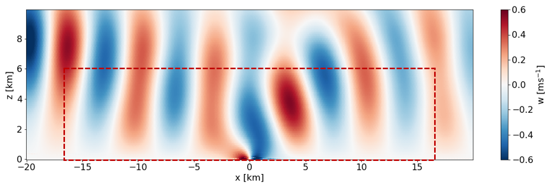
Figure 1 Vertical velocity contours of the flow over a small hill located at x=0 km, produced by simulating a bell-shaped hill under linearly stratified laminar conditions using the Simulator for Wind Farm Applications (SOWFA). The region outside the dotted red box consists of Rayleigh damping layers at the inlet (left), top, and outlet (right).

The current approaches to setting up RDLs in wind farm simulations are rather ad hoc. Extensive fine-tuning of the damping parameters is required to set up a working simulation, which may be applicable only to a specific case (Allaerts, 2016; Lanzilao and Meyers, 2023). As a result, setting up reflection-free simulations is tedious, computationally expensive, and time-consuming. The aim of this paper is to investigate how to make the process less ad hoc by investigating relationships between the simulation setup and the fundamental physical parameters driving wind farm flow under stable atmospheric conditions.

3 Flow scenarios

In this study, we consider two simple 2D flow scenarios that generate internal gravity waves: the flow over a bell-shaped hill and the flow through a wind farm canopy. Our initial focus lies on the hill case, which is used in various meteorology and earth sciences studies, such as Vosper and Ross (2020) and Snyder et al. (1985). The reasons for starting with the hill case include the simplicity of the flow scenario, computational affordability, and the availability of a semi-analytical solution (which is useful for validation purposes). Moreover, the primary aim of this study is how best to handle atmospheric gravity waves in numerical simulations, and the wave source is thereby of less importance. Nevertheless, the simulated hill heights are similar to typical wind turbine rotor tip heights, and the half width of the hill is of the same order as typical wind farm lengths. In the second flow case, we study the flow through wind farm canopies to extend the findings from the hill case to wind farm applications. Unlike the rigid hill, a wind farm canopy is a porous region in which the drag force of the wind turbines is applied homogeneously. The details of both flow scenarios are discussed in more detail in the following subsections.

3.1 Scenario 1: bell-shaped hill

The first flow scenario considers flow over a 2D bell-shaped hill. The height profile h of a bell-shaped hill – sometimes referred to as the witch of Agnesi (WOA) profile – is defined in the horizontal direction x as

$$\begin{array}{}\text{(4)}& {\displaystyle }h\left(x\right)={\displaystyle \frac{H}{\mathrm{1}+(x/L{)}^{\mathrm{2}}}}.\end{array}$$

This profile is governed by two parameters, i.e., the maximum hill height H and the half width at half height L.

To allow for a direct comparison between an LES and a linear gravity wave potential flow solution, surface friction and the Coriolis force were excluded, and only a linearly stratified free atmosphere was considered with uniform inflow. Although the inflow was laminar, the LES model could still generate turbulence due to flow separation behind the hill.

A computationally inexpensive semi-analytical flow solution over the hill was used to understand the properties of the IGWs and validate the numerical solutions. We use the analytical solution along with the relative root mean square error (R-RMSE) metric (discussed in Sect. 4.3) to quantify reflections in the simulations. The following subsection gives an overview of this semi-analytical solution and how it is used in this study.

3.1.1 Semi-analytical solution

Linear wave theory, particularly the Taylor–Goldstein equations, is commonly used to study atmospheric gravity waves. Allaerts (2022) used these equations to develop a Python module called Linear Buoyancy Wave Package (LBoW) to solve linear buoyancy wave problems. In this research, we use part of this code that computes a semi-analytical steady-state solution of the uniform, stratified flow over the WOA hill. The code solves the equations on a grid in frequency space using fast Fourier transform (FFT). The solution is independent of the grid size in the vertical direction but not in the horizontal direction. A solution at any vertical level can be acquired without requiring a prior solution at lower and higher levels. The grid resolution in the horizontal direction dictates the solution accuracy. The FFT solution deviates from a theoretical Fourier transform of the bell-shaped hill for high horizontal wave numbers due to rounding errors. A mesh size in the range of 20 to 100 m is recommended to compute the semi-analytical solution.

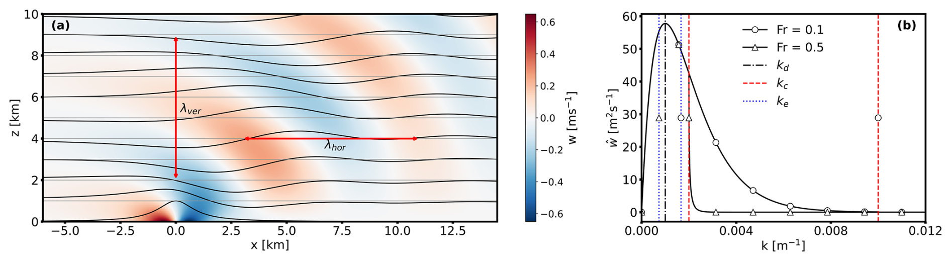
Figure 2 (a) Steady-state analytical solution of flow over a WOA hill centered at x=0 km. The color contours represent vertical velocity, and the streamlines from the displacement field show the wave propagation. (b) The streamwise wave spectrum for vertical velocity at a height, where critical, dominant, and effective wave numbers are identified for Fr=0.1 and 0.5. Figure created with LBoW (Allaerts, 2022).

The steady-state, semi-analytical solution of uniform flow over the hill in a stably stratified free atmosphere with a uniformly increasing potential temperature with height is shown in Fig. 2a, where the upward flow deflection by the hill triggers only IGWs. The vertical velocity contour and streamlines of the displacement field clearly show the propagation of gravity waves in the vertical direction. The gravity waves transport energy mainly upward from their source, the hill or a wind farm, but some wave amplitude decays with height. At the same time, the waves are also blown downstream. The combined effect is a decrease in the amplitude of some parts of the wave with height and downstream distance. The properties of IGWs depend on the wind speed U, hill half width at half height L, hill maximum height H, and Brunt–Väisälä frequency $N=\sqrt{(g/\mathit{\theta })\left(\frac{\mathrm{d}\mathit{\theta }}{\mathrm{d}z}\right)}$ (where g is acceleration due to gravity and θ is the potential temperature at height z). Employing similarity theory, we normalize these variables to get two physical parameters, the Froude number (Fr) and the slope parameter (S_h), where Fr = $U/NL$ and S_h = $H/L$. Thus, the wave properties depend mainly on the free atmosphere Froude number and the slope parameter.

It is important to understand that the wave train seen in Fig. 2a is not monochromatic but is actually a wave spectrum, which is given by the following expression:

$$\begin{array}{}\text{(5)}& \widehat{w}(k,z)=\mathit{\pi }HLiUk{e}^{-\left|k\right|L}{e}^{imz},\end{array}$$

with

$$\begin{array}{}\text{(6)}& m\left(k\right)=\left\{\begin{array}{ll}\text{sgn}\left(k\right)\sqrt{k_{\mathrm{c}}^{\mathrm{2}}-k^{\mathrm{2}}}& \text{for}\left|k\right|<k_{\mathrm{c}},\\ i\sqrt{k^{\mathrm{2}}-k_{\mathrm{c}}^{\mathrm{2}}}& \text{for}\left|k\right|>k_{\mathrm{c}},\end{array}\right.\end{array}$$

where k and $k_{\mathrm{c}}=N/U$ are horizontal and critical wave numbers, respectively. Here, sgn suggests the use of the actual value, positive or negative, acquired from the square root in the expression, as Eq. (5) includes imaginary numbers. The spectrum for a specific height is shown in Fig. 2b together with the three important length scales corresponding to the dominant ($k_{\mathrm{d}}=\mathrm{1}/L$), critical (k_c), and effective ($k_e=\mathrm{1}/{\mathit{\lambda }}_{\mathrm{hor}}$) wave numbers. Thus, there are three important wavelengths to consider:

1. The wavelength with the highest amplitude is the dominant wavelength, λ_L=2πL, which depends on the hill width.

2. However, the dominant wavelength for the bell-shaped hill is not necessarily the wavelength that is the most visually apparent in contour plots. For example, the most apparent wavelength, which is termed the effective wavelength, is shown in Fig. 2a with a horizontal red arrow and is labeled λ_hor.

3. Lastly, there is a critical wavelength (often we consider its reciprocal, the critical wave number). For wavelengths smaller (or wave numbers larger) than the critical one, the waves cannot be supported by buoyancy, so they dissipate and are called “evanescent” waves.

Figure 3 The variation in effective (a) horizontal and (b) vertical wavelengths with Fr.

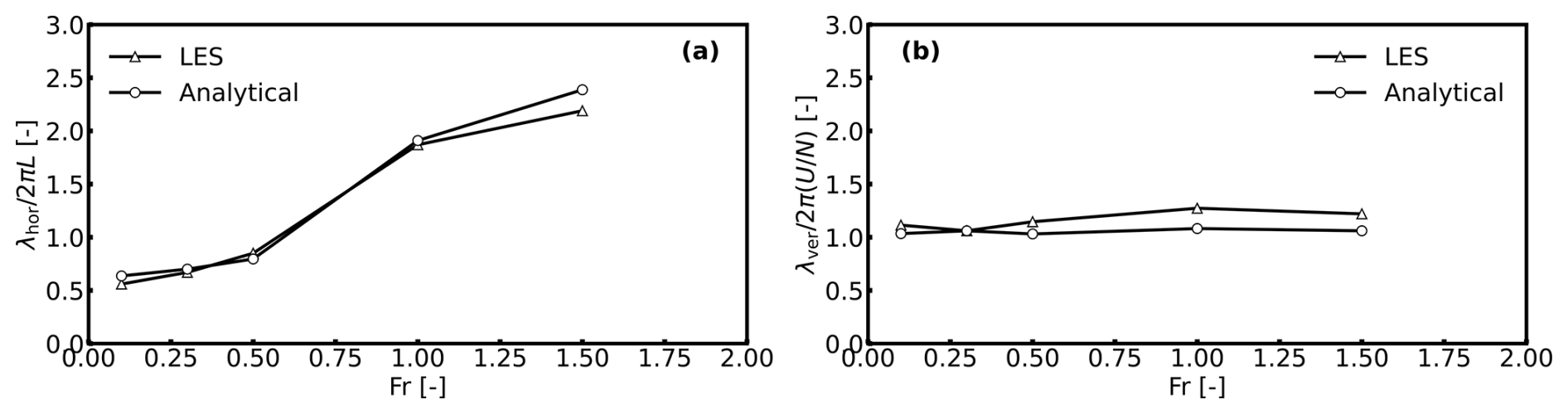
Although the analytical solution tells us that wave amplitude depends more on the hill slope, particularly the height, the effective wavelengths and the inclination angles of the IGWs depend on Fr. The IGWs naturally tend to travel vertically, but the background flow forces them to bend. Since zero advection speed is impossible, these waves always travel inclined. For Fr in the range of 0.1 to 1.5, the inclination angle to the streamwise direction, estimated from the vertical velocity field, is in the range of 75–53°, respectively. The effective horizontal wavelength (λ_hor) is sensitive to the hill width for low Fr, but for Fr>0.5, it depends more on the Scorer parameter ($N/U$), which is the reciprocal of the buoyancy length. This can be seen in Fig. 3a, where the normalized λ_hor, calculated from the semi-analytical solution and LES, is plotted against Fr. We measure λ_hor as twice the distance between the global maxima and minima determined from a vertical velocity plot at a constant height along the domain length. We see that as Fr is increased, λ_hor increases, but it is not a linear relation.

Although we visually identify with the effective wavelength of AGWs when we view figures like Fig. 2a, those AGWs are really a spectrum of waves. Based on the spectrum and wave numbers shown in Fig. 2b, the situation can be classified into two different conditions:

1. When the critical wave number is greater than k_d or when Fr<0.5, the dominant wavelength is greater than λ_hor. In this situation, λ_hor depends more on the hill half width than on the Scorer parameter, and the entire wave spectrum is preserved, and the waves propagate.

2. On the other hand, when Fr>0.5, the critical wave number is closer to k_d; thus, part of the spectrum becomes evanescent, and wave numbers greater than k_c are dissipated. In this case, the dominant wavelength is less than λ_hor, which depends more on the Scorer parameter.

The effective vertical wavelength (λ_ver), shown as the vertical red arrow in Fig. 2a, depends only on the Scorer parameter, which is proportional to the vertical wave number. This is evident from Fig. 3b, where λ_ver, normalized with the maximum vertical wavelength $\mathrm{2}\mathit{\pi }(U/N)$, is shown as a function of Fr. The constant ${\mathit{\lambda }}_{\mathrm{ver}}/\mathrm{2}\mathit{\pi }(U/N)$ for varying Fr indicates that λ_ver does not depend on L and is usually representative of the maximum vertical wavelength. λ_ver is measured as twice the distance between the global maxima and minima determined from a vertical velocity plot along the domain height at the x location corresponding to H. The locations of global extrema are extracted from the vertical velocity on the physical coordinates such that grid stretching does not affect λ_ver. It is also important to note that the IGWs curve downstream of the hill; thus, λ_ver varies slightly at different streamwise locations for values of Fr>0.5, as seen in Fig. 3b. Therefore, the maximum vertical wavelength is better suited to scaling in the vertical direction, especially since it is almost equal to λ_ver.

Hence, it can be seen that the effective horizontal and vertical wavelengths can be greater than the dominant length scales, i.e., the hill width and height; thus, domains scaled with the hill width and height might be inappropriate for the accurate simulation of gravity waves.

This study focuses only on the Froude number as it pertains to gravity wave properties that are critical to the simulation setup. The slope parameter is less critical for this research, and the slope of the hill (S_h) is kept the same. With different hill shapes, the amplitude and wave spectrum would change, making comparisons between simulations with different hill shapes inconsistent. In addition, we only consider the steady-state solution.

3.2 Scenario 2: wind farm canopy

Wind farm flow interactions with the atmosphere involve a wide range of length scales. When focusing on wind-farm-induced IGWs, large length scales are important, as the expected IGW wavelengths are on the scale of the wind farm length, which can be several kilometers. Since the intra-farm (turbine–wake) interactions are not the focus of this study, wind farm canopies are a convenient way to model wind farms without the complexity of modeling individual wind turbines. The concept of a wind farm canopy was introduced by Markfort et al. (2018) through an analytical model to represent large wind farms in weather prediction models. In our work, we use a similar approach to simulate the cumulative drag force of a wind farm consisting of a number of wind turbines of a given type.

The standard coefficient of thrust associated with a wind turbine rotor is

$$\begin{array}{}\text{(7)}& C_{\mathrm{t}}={\displaystyle \frac{\mathit{T}}{\frac{\mathrm{1}}{\mathrm{2}}\mathit{\rho }{\mathit{U}}^{\mathrm{2}}{A}_{\mathrm{r}}}}={\displaystyle \frac{\mathit{T}}{\frac{\mathrm{1}}{\mathrm{2}}\mathit{\rho }{\mathit{U}}^{\mathrm{2}}\mathit{\pi }\frac{D_{\mathrm{r}}^{\mathrm{2}}}{\mathrm{4}}}},\end{array}$$

where A_r is the rotor-swept area, D_r is the turbine rotor diameter, ρ is the density of air, T is the dimensional rotor thrust force, and U is the freestream velocity. Because we distribute the force of the rotors in the wind farm over the volume occupied by the wind farm, it is better to define a thrust coefficient based on the area of the farm belonging to this rotor (i.e., the entire footprint area considering turbine spacing allocated to this wind turbine). This area is $A_{\mathrm{f}}=\left(S_x{D}_{\mathrm{r}}\right)\left(S_y{D}_{\mathrm{r}}\right)=S_x{S}_y{D}_{\mathrm{r}}^{\mathrm{2}}$, where S_x and S_y are the turbine spacings in the two horizontal directions within the farm. This new thrust coefficient is

$$\begin{array}{}\text{(8)}& c_{\mathrm{t}}={\displaystyle \frac{\mathit{T}}{\frac{\mathrm{1}}{\mathrm{2}}\mathit{\rho }{\mathit{U}}^{\mathrm{2}}{S}_x{S}_y{D}_{\mathrm{r}}^{\mathrm{2}}}}.\end{array}$$

The two thrust coefficients are related to each other through

$$\begin{array}{}\text{(9)}& c_{\mathrm{t}}={\displaystyle \frac{\mathit{\pi }}{\mathrm{4}{S}_x{S}_y}}{C}_{\mathrm{t}}.\end{array}$$

Defining dimensional thrust based on c_t, we have

$$\begin{array}{}\text{(10)}& \mathit{T}={\displaystyle \frac{\mathrm{1}}{\mathrm{2}}}\mathit{\rho }{\mathit{U}}^{\mathrm{2}}{S}_x{S}_y{D}_{\mathrm{r}}^{\mathrm{2}}{c}_{\mathrm{t}},\end{array}$$

and normalizing dimensional thrust by the volume of the farm occupied by a turbine, $V_{\mathrm{f}}=S_x{S}_y{D}_{\mathrm{r}}^{\mathrm{2}}(H_{\mathrm{t}}-H_{\mathrm{b}})$, where H_t and H_b are the height of the top and bottom of the turbine rotor and also the height of the top and bottom of the wind farm canopy, we have

$$\begin{array}{}\text{(11)}& \begin{array}{rl}{f}_{\mathrm{wf}}& ={\displaystyle \frac{\mathit{T}}{V_{\mathrm{f}}}}={\displaystyle \frac{\mathrm{1}}{\mathrm{2}}}{\displaystyle \frac{\mathit{\rho }{\mathit{U}}^{\mathrm{2}}{S}_x{S}_y{D}_{\mathrm{r}}^{\mathrm{2}}}{S_x{S}_y{D}_{\mathrm{r}}^{\mathrm{2}}(H_{\mathrm{t}}-H_{\mathrm{b}})}}{c}_{\mathrm{t}}={\displaystyle \frac{\mathrm{1}}{\mathrm{2}}}{\displaystyle \frac{\mathit{\rho }{\mathit{U}}^{\mathrm{2}}}{(H_{\mathrm{t}}-H_{\mathrm{b}})}}{c}_{\mathrm{t}}\\ & ={\displaystyle \frac{\mathrm{1}}{\mathrm{8}}}{\displaystyle \frac{\mathit{\rho }{\mathit{U}}^{\mathrm{2}}\mathit{\pi }}{S_x{S}_y(H_{\mathrm{t}}-H_{\mathrm{b}})}}{C}_{\mathrm{t}}.\end{array}\end{array}$$

It is this thrust per unit volume that is applied to the momentum equations as a source term within the wind turbine canopy volume. The wind speed, U, is determined locally at each cell center within the canopy.

4 Methods

4.1 Simulation parameters and setup

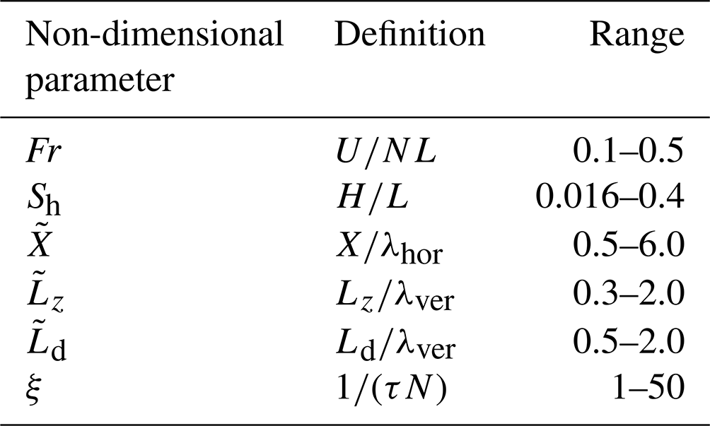
A set of non-dimensional parameters governs the flow over the terrain and through wind farms under linearly stratified atmospheric conditions. These parameters can be determined by normalizing the flow equations or performing dimensional analysis of a number of key variables. These variables are detailed in Table 1, along with their practical values in wind energy applications. From these variables, the set of non-dimensional parameters in Table 2 can be defined. The first two sets are physical parameters, namely the Froude number and slope parameter, while the remainder are simulation parameters.

An appropriate choice of grid structure, resolution, and time step is important for the simulation of gravity waves, particularly for very low values of Fr, because the flow interactions can trigger subgrid-scale wavelengths. Likewise, the frequencies of some waves in the spectrum could be shorter than the simulation time steps, leading to an unresolved fraction of the spectrum. However, the relevant value of Fr for wind farm applications is approximately between 0.1 and 0.5, for which a grid independence study was carried out. It was found that grid resolutions, roughly 10 m in all directions, used in wind farm LES to resolve wind turbines and their wakes are more than sufficient to resolve wind-farm-induced AGWs.

Table 1 Key variables in the simulation of atmospheric gravity waves under linearly stratified free atmospheric conditions with typical ranges in wind energy applications.

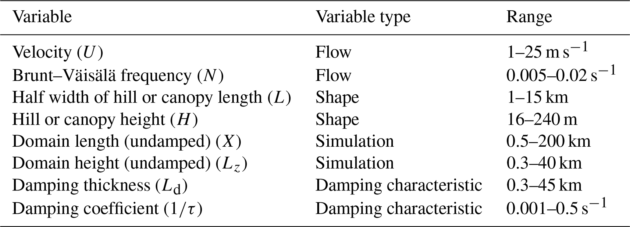
Table 2 Non-dimensional parameters derived from the variables in Table 1 with typical ranges.

LES of flow over the WOA hill and through the wind farm canopy is carried out with the Simulator for Wind Farm Applications (SOWFA) Churchfield et al. (2012). Based on OpenFOAM, this code is mainly used for the LES of atmospheric flows over terrain and through wind farms, where a one-equation model is commonly used for subgrid-scale turbulence modeling. SOWFA has actuator models for wind turbine aerodynamics that can be coupled with aero-servo-elastic tools. Moreover, it can use boundary inflow data from mesoscale weather data, and terrain can be included through non-conformal meshes. The model setup solves the incompressible Navier–Stokes equations under non-hydrostatic conditions and with the Boussinesq approximation for buoyancy. Equations for continuity, momentum, and potential temperature are those typically used in the LES of atmospheric flows. A more complete description is given in Churchfield et al. (2012). For simulations with the wind farm canopy, the drag force of the wind farm is added to the momentum equation as a body force. Rayleigh damping is applied as a body force in the forcing zones through the momentum equation, the details of which are given in the following subsection.

Figure 4 shows the numerical setup for the hill and wind farm canopy cases. The flow is driven in and out of the domain by inflow–outflow boundary conditions. Periodic boundary conditions are used in the transverse direction only. Because SOWFA's inflow and outflow boundary conditions and lower and upper impenetrable boundaries set the velocity flux locally over each boundary face, there is no need for pressure boundary conditions (keeping in mind that the pressure solve in an incompressible code enforces continuity). To simplify the setup, wind shear is neglected, a uniform inflow is imposed as the inlet boundary condition for wind speed, and the zero-gradient boundary condition is implemented at the outlet. In addition, free-slip boundary conditions are imposed at the top and bottom of the domain. The temperature profile is linear in the vertical direction, giving a constant Brunt–Väisälä frequency with height. There is no heat flux at the ground. Moreover, Coriolis forces are not considered. These conditions are intended to mimic those of a stable free atmosphere without the ABL and inversion layer.

A surface profile for the WOA hill is created using a Python script, and the computational mesh conforms to the hill. A mesh with layered refinement is used with $\mathrm{20}\mathrm{m}\times \mathrm{20}\mathrm{m}\times \mathrm{20}\mathrm{m}$ resolution in the non-damped domain and $\mathrm{40}\mathrm{m}\times \mathrm{20}\mathrm{m}\times \mathrm{40}\mathrm{m}$ in the top damping layer. The first mesh layer near the surface ends in the top damping layer to ensure any numerical noise for switching to a coarser mesh is damped. The domain for all cases is 100 m in the y direction, whereas the x and z extents are varied as a function of the effective horizontal and vertical wavelengths, respectively, as the domain length and height are critical simulation variables when simulating gravity waves. The exact domain length and height used for each simulation are reported while discussing the results. Both the hill and the wind farm canopy are extended in the transverse direction to the sides of the domain, effectively creating an infinite ridge and a semi-infinite wind farm, respectively, as we are primarily interested in vertical and streamwise flow.

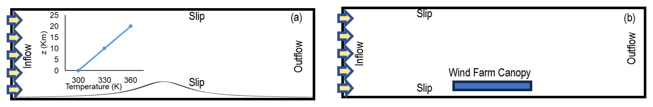
Figure 4 Lateral view of the simulation setup: (a) with a schematic WOA hill profile and (b) with a schematic wind farm canopy.

The guidelines to systematically model AGWs can be established based on the hill scenario; however, the characteristics of the AGWs may vary for a porous wind farm canopy as opposed to a solid hill. Therefore, wind farm canopies are simulated to extend the findings from the hill scenario to the wind farms. This approach reduces computational resources, which is desirable as hundreds of cases are run to evaluate the extent of wave reflections. The wind farm canopy model can be used with relatively coarse grids compared to conventional actuator models that resolve wind turbines to a given extent. The numerical setup with the wind farm canopy is the same as that of the WOA hill, except that the hill is replaced with wind farm drag as a body force.

4.2 Rayleigh damping

RDLs are implemented as zones adjacent to the reflective boundaries in the simulation domain and far from the region of interest, such as a wind farm. It is critical to note that RDLs are always implemented in the free atmosphere because it is the gravity waves in the free atmosphere that reflect from the boundaries. The primary role of an RDL is to dissipate the energy propagated through the zone by AGWs. In this study, only the vertical velocity is damped, unless mentioned otherwise, as the prominent perturbation is the vertically deflected velocity by the hill or the wind farm canopy. If periodic streamwise boundary conditions are used, an RDL is implemented at the top boundary only with an RDL-like fringe region at the outlet where flow is recycled to the inlet. However, in a simulation setup with inflow–outflow boundary conditions, RDLs may be required at various boundaries. The RDL at the inlet will filter any incoming turbulence. Generally, damping incoming turbulence into the boundary layer is undesirable in wind farm simulations; however, in this study, for simplicity, we have neglected inflow turbulence. This should not impact the aim of the study, which is to minimize gravity wave reflections efficiently.

4.3 Quantifying reflections

Reflectivity is quantified by the method proposed by Allaerts and Meyers (2017), which is a modification of the procedure initially given by Taylor and Sarkar (2007). The reflection coefficient (Cr) is one of two primary tools used here to analyze the simulation data, and its calculation can be summarized in the following two steps. First, the vertical velocity values on a vertical streamwise plane are converted to horizontal and vertical wave number space (K_s and M_s, respectively) through a 2D Fourier transform. The wave number coordinates centered at 0 are similar to the physical coordinates, where K_s and M_s are on the horizontal and vertical axes, respectively. The upward- and downward-moving waves are separated based on the quadrants they fall into. The upward-propagating waves are in the first and third quadrants, whereas the downward-propagating waves are in the second and fourth quadrants on the K_s and M_s coordinates. Thus, only the Fourier coefficients in quadrants I (i.e., $K_{\mathrm{s}},M_{\mathrm{s}}>\mathrm{0}$) and III (i.e., $K_{\mathrm{s}},M_{\mathrm{s}}<\mathrm{0}$) are retained for upward waves, and those in the other two quadrants are set to zero. Likewise, quadrants II (i.e., $K_{\mathrm{s}}<\mathrm{0},M_{\mathrm{s}}>\mathrm{0}$) and IV (i.e., $K_{\mathrm{s}}>\mathrm{0},M_{\mathrm{s}}<\mathrm{0}$) are retained for the downward waves. The filtered coefficients are inverse transformed to obtain the respective velocity fields, as shown in Fig. 5. The tilted phase fronts on these contours clearly show (a) the initial upward-propagating waves and (b) the much weaker reflected downward-propagating waves. Wave energy propagates normal to the phase fronts and is calculated from these decomposed vertical velocity fields. Finally, the reflection coefficient is estimated by taking the ratio of total downward- to upward-propagating energy. This Cr metric sometimes gives inconsistent values, especially for low Fr and L, possibly because the spectrum includes a large fraction of high-frequency waves. Therefore, visual inspection of the simulation fields, especially the vertical velocity, is critical to ensure that the value predicted is realistic; improving or replacing this metric is left for future work.

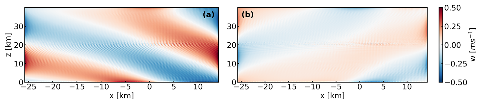
Figure 5 Decomposed vertical velocity fields for a WOA hill simulation showing (a) upward- and (b) downward-propagating internal waves.

In the case of the hill, the numerical solution can be compared to the semi-analytical solution using the relative root mean square error (R-RMSE) metric. The differences between the vertical velocity (w) fields from the numerical and analytical solutions are normalized with the maximum w from the analytical solution to determine the R-RMSE over a vertical plane in the streamwise direction. The vertical velocity is always taken at time t when $t=\mathrm{300}/N$, which is equivalent to 2.083, 4.167, or 8.33 h for $N=\mathrm{0.02},\mathrm{0.01}$, and 0.005 s⁻¹, respectively. As the R-RMSE metric depends on the number of points sampled, we only calculated this for the same section of the domain, around the hill or canopy. This has the drawback of not capturing reflections close to the boundaries. However, the R-RMSE can be better than Cr in capturing localized spurious wave sources, like numerical noise at the interface of the damping layers with the non-damped domain. Due to the strengths and weaknesses of the two metrics, we analyze the results of both, and it is found that the R-RMSE metric generally detects the same patterns seen in Cr. Therefore, only results in Cr are reported in the paper to be consistent with the literature. In all cases, unless otherwise mentioned, the vertical velocity values are taken from a vertical plane at the mid-point of the domain. For reflection-free simulations, we require that the criterion of Cr and R-RMSE <10 % should be met.

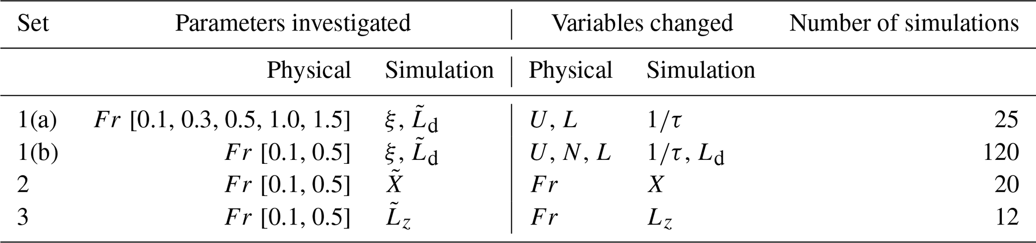
4.4 Simulation sets

Simulations were run initially to acquire a base case, which was then used to explore the dependency of reflection on the non-dimensional parameters defined in Table 2. Various combinations of damping layers with different combinations of characteristics were simulated to investigate the most appropriate configuration with minimum reflections. Details on the configurations explored are given in the Appendix. In addition to exploring the configuration of the damping layers, three simulation sets are defined, as detailed in Table 3. These three simulation sets were repeated for the wind farm canopy.

• The first set of simulations investigates the impact of damping characteristics on reflections and their optimal values for a range of Fr. Set 1(a) explores the extent of reflections when varying the damping coefficient for a range of Fr values, i.e., 0.1 to 1.5, where Fr was adjusted by changing U and L. In Set 1(b), the damping coefficient and thickness were changed when setting Fr=0.1 and 0.5, where Fr was adjusted by changing N and U or U, N, and L, ensuring dynamically similar solutions.

• Set 2 explores the impact of the domain length on wave reflections. In this case, the domain length was varied for two values of Fr.

• Set 3 investigates the impact of domain height on wave reflections. In this case, for two values of Fr, the domain height was varied in proportion to the expected λ_ver.

Table 3 Simulation sets.

5 Results

5.1 Hill

This section first considers the optimum damping configuration for the hill case as a baseline before moving on to the wind farm canopy setup.

5.1.1 Configuring the damping layers

Correctly setting up the size and location of the damping layers is important for the accurate and effective simulation of AGWs. Therefore, we test various configurations of the damping layers that give minimum reflections and use these as a base case for further investigation of the sensitivity to the non-dimensional parameters. As mentioned earlier, we require that both Cr and R-RMSE be less than 10 % for the simulation to qualify as reflection-free, as defined in this study. Following a brief investigation of various combinations of damping layers, it was found that RDLs at the inlet, outlet, and top boundaries give minimum reflections, and thus all subsequent simulations use this configuration as the base case.

5.1.2 Dynamic similarity

We started the analysis by testing whether the non-dimensional parameters discussed in Sect. 4.1 are sufficient to ensure dynamic similarity; i.e., the non-dimensional solution remains the same if the non-dimensional parameters are the same, irrespective of the values of the variables defining them. The simulations performed had a setup with a damping layer thickness and domain height 1.5 times the effective vertical wavelength and a domain length 5 times the expected effective horizontal wavelength. Figure 6 shows the dependency of wave reflections on the non-dimensional damping parameter, ξ for changing buoyancy and hill half widths ($U/N$ and L), and buoyancy and advection timescales ($\mathrm{1}/N$ and $L/U$). In terms of minimizing reflections, the plots indicate that a suitable range for ξ is between 1 and 10 when Fr=0.1, and the buoyancy timescale is an appropriate scaling parameter for the damping coefficient. The plots further show that the results are independent of both the timescale and the length scale because the solutions are dynamically similar. The buoyancy length was kept constant (i.e., $U/N=\mathrm{0.5}$ km) by changing the Brunt–Väisälä frequency and inflow velocity for a constant hill half width (i.e., L=5 km). Thus, the advection timescale was different for these two cases. The buoyancy length was varied by adjusting the Brunt–Väisälä frequency and hill half width to fix Fr=0.1, and the buoyancy timescale and physical length scale were also varied. Thus, it is deduced that from the definition $\mathit{Fr}=U/NL$, $L/U$ acts like N or the free atmosphere's stability. This means that the stability of the free atmosphere is relative to the size of the disturbance source and the geostrophic wind. These three cases can be compared in different ways, which can establish dynamically similar solutions for all comparisons. Similar results are seen for Fr=0.5, though these are not shown for clarity.

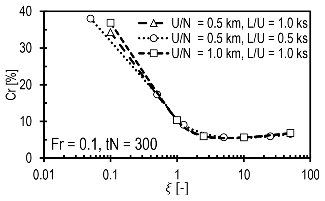
Figure 6 Reflection coefficient as a function of normalized damping coefficient ξ for varying length scales and timescales.

5.1.3 Optimal damping coefficient as a function of Froude number

In general, very low damping coefficients lead to the highest reflections; however, very high damping coefficients, e.g., ξ≫10, also enhance reflections as the IGWs reflect off the damping layer instead of the boundaries. These effects can be seen in Fig. 7. Strong reflections and energy accumulation can be seen visually in Fig. 7 (top) for ξ=0.1, where they appear parallel to the inlet on the left and gradually contaminate the solution in the entire domain. Figure 7 (middle) shows vertical velocity contours when ξ=10, which are the least affected by reflections and energy accumulation at the inlet. Moreover, the gradual decay of IGWs with height inside the top RDL is evidence of suitable damping characteristics. On the other hand, Fig. 7 (bottom) shows vertical velocity contours when ξ=50, where IGWs are abruptly attenuated right at the start of the top damping layer. Moreover, accumulated waves appear at the end of inflow RDL as if it were a hard boundary.

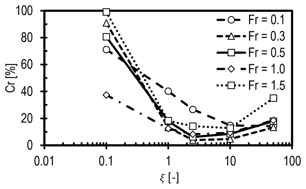
It was shown in Sect. 5.1.2 that the optimal damping coefficient for Fr=0.1 is around 10. However, Fig. 8 shows that for values of Fr>0.1, the optimal damping coefficient is somewhat less, with minimum reflections occurring for values of ξ between 2 and 10, although the sensitivity to ξ in this range is small. The adverse level of reflection for low and very high damping coefficients is also apparent from this plot. For Fr=0.1 and 1.5, Cr cannot be made less than 10 % because the damping layer thickness is just one vertical wavelength, which is insufficient for these very low and supercritical values of Fr, respectively. These simulations had damping layer thicknesses and domain heights equal to the effective vertical wavelength, and the domain length was twice the effective horizontal wavelength. Supercritical values of Fr (Fr>1), a regime in which much of the wave content is evanescent, are less likely to occur for large wind farms, whereas low Fr values are very likely. For this reason, the following sections restrict analysis to the expected upper and lower ranges of the Froude number for wind energy applications; i.e., Fr=0.1 and 0.5.

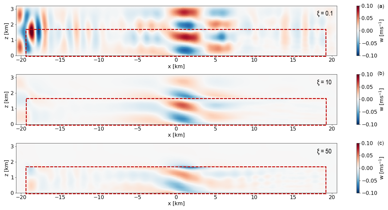
Figure 7 Contours of vertical velocity in a streamwise-oriented vertical plane at tN=300 for Fr=0.1 with ξ=0.1 (a), ξ=10 (b), and ξ=50 (c). The red box shows the non-damped domain, and everything outside is the RDL.

Figure 8 Reflection coefficient as a function of ξ for a range of Froude numbers.

5.1.4 Impact of damping layer thickness on reflections

So far, we have considered the impact of ξ on the reflections while L_d is equal to or greater than the vertical wavelength. However, the impact of damping characteristics on reflections is coupled. A weak, thick damping layer may have the same impact as a strong, thin layer. Therefore, determining the coupled impact of the damping characteristics on reflections and the minimum damping thickness is desirable, as knowing the minimum effective damping layer thickness can help reduce the computational load.

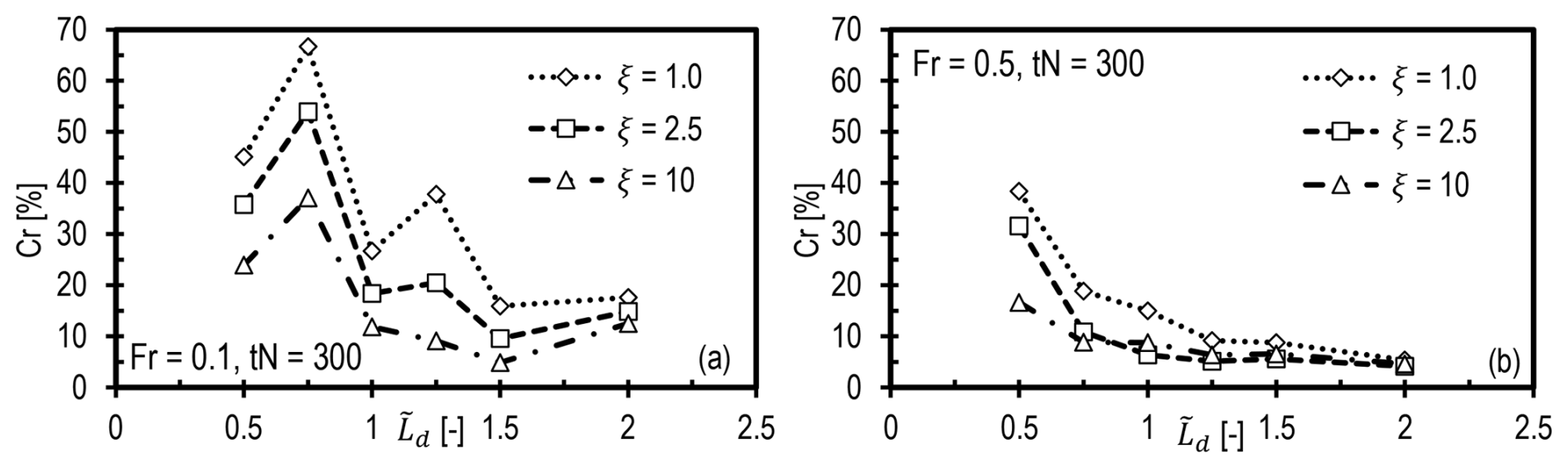
Figure 9 Reflection coefficient for the hill case as a function of normalized damping layer thickness for different values of the damping coefficient when (a) Fr=0.1 and (b) Fr=0.5.

The joint effect of different damping parameters is investigated for Fr=0.1 and Fr=0.5, where the damping thickness and coefficient are varied simultaneously. In general, thicker damping layers for all damping coefficient values should reduce reflections, but thinner damping layers are desirable for their low computational cost. Figure 9 shows that a damping layer set to the optimal damping coefficient and accommodating one effective vertical wavelength seems more effective than a thicker layer with a sub-optimal value of ξ. Figure 9a shows that Cr is minimum for all values of ${\stackrel{\mathrm{̃}}{L}}_{\mathrm{d}}$ when ξ is 10. The non-monotonic nature of the plots in this figure indicates how optimizing the setup for a low value of Fr is more challenging. The exact reason for this non-monotonic behavior is hard to establish, but it is most likely associated with the complicated wave properties for low values of Fr. For instance, wavelengths become shorter for low Fr. Thus, the resolved wave spectrum can vary significantly for even small changes in the domain size, which is linked to the amount of wave reflection. Furthermore, the waves are more aligned to the horizontal for a low value of Fr, complicating the interaction with the background advecting flow as the wavefronts are more directly aligned with the inlet wind flow than that of a higher-Fr case. Moreover, the energy accumulation is higher for a low value of Fr as the wave speed is faster than the advection speed, in turn causing more contamination of the solution. This also suggests inadequacy of the RDLs in terms of their ability to prevent energy accumulation at the inlet only, delaying its propagation back into the domain.

Figure 9b shows monotonic reflection behavior for Fr=0.5. It can be seen that a value of ξ=2.5 provides an optimal solution when ${\stackrel{\mathrm{̃}}{L}}_{\mathrm{d}}>\mathrm{1.0}$, and a value of ξ=10 is best when ${\stackrel{\mathrm{̃}}{L}}_{\mathrm{d}}<\mathrm{1.0}$. The damping layer thickness required when Fr=0.1 is slightly bigger than that for Fr=0.5 to limit the reflections to the same levels. This can be seen when comparing the optimal setups for Fr=0.1 and Fr=0.5, where Cr is limited to 5 %, whereby ${\stackrel{\mathrm{̃}}{L}}_{\mathrm{d}}$ is 1.2 for Fr=0.5 and ${\stackrel{\mathrm{̃}}{L}}_{\mathrm{d}}$ is 1.5 for Fr=0.1.

In summary, the damping layer thickness should be greater than one effective vertical wavelength to efficiently damp the IGWs. This aligns with the recommendation of Klemp and Lilly (1978) but is based on analyzing the entire wave spectrum instead of analyzing individual wave numbers, which was their approach.

5.1.5 Domain length impact on reflections

Intuitively, the location of the top boundary is more important than that of the other boundaries, as the gravity waves travel upward, and reflections are mainly expected from the top boundary. However, the accumulation of energy at the inlet boundary, shown in Figs. 1 and 7, indicates the importance of appropriately positioning the inlet and outlet relative to the hill or wind farm (i.e., the zone of interest). One approach is to place boundaries far from the zone of interest to prevent spurious waves from affecting the flow around the zone of interest. This approach has two major flaws: it is costly in terms of computational resource for LES studies, and simulations can run only for a limited time before the reflections reach the zone of interest. This constraint conflicts with the common practice in wind farm LES of simulating several domain flow-through times to obtain reliable statistics. Moreover, the contamination of the solution upstream of a wind farm may affect the inflow, and an unrealistic inflow to the wind farm would lead to an unreliable solution. Therefore, knowing the shortest possible domain length that ensures the least contaminated inflow approaching the zone of interest is important to produce accurate solutions and save computational resources and time. To this end, a set of simulations, denoted in Table 3 as Set 2, was performed for values of Fr=0.1 and Fr=0.5, where the domain length was varied between 0.5λ_hor and 4.0λ_hor. Instead of simulating for several different values of the damping parameters, we used the results from Sect. 5.1.4 with ξ=10 for Fr=0.1 and ξ=2.5 for Fr=0.5. The value of ${\stackrel{\mathrm{̃}}{L}}_{\mathrm{d}}$ was set to 1.5 for Fr=0.1 and 1.2 for Fr=0.5.

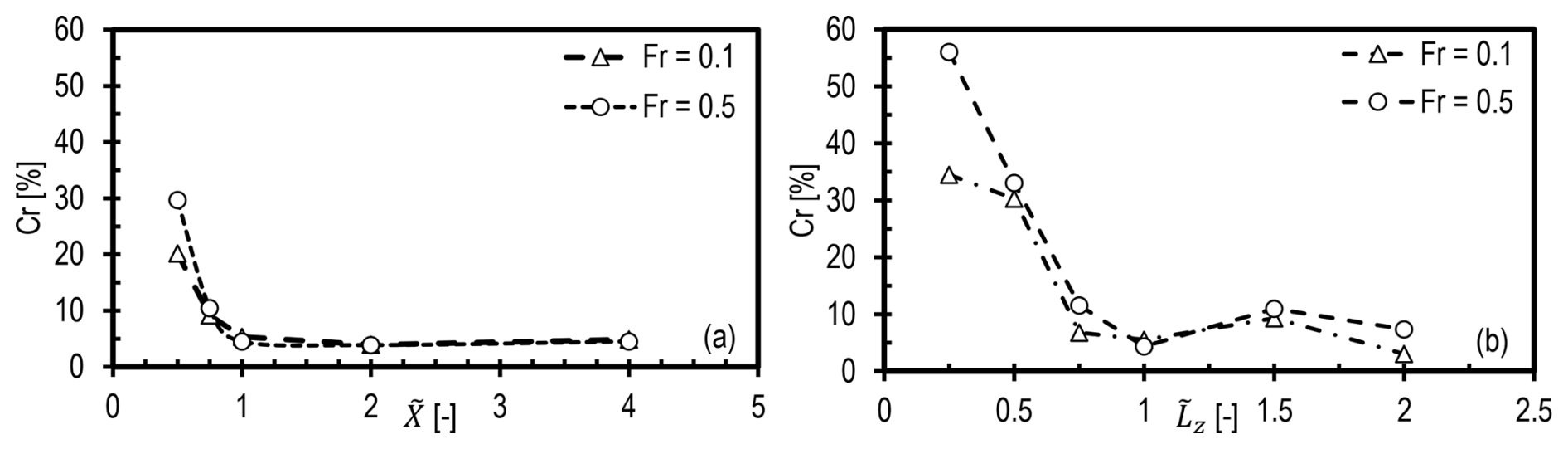
Figure 10 Reflection coefficient for the hill case as a function of (a) domain length for Fr=0.1 and Fr=0.5 and (b) domain height for Fr=0.1, ${\stackrel{\mathrm{̃}}{L}}_{\mathrm{d}}=\mathrm{1.5}$ and Fr=0.5, ${\stackrel{\mathrm{̃}}{L}}_{\mathrm{d}}=\mathrm{1.2}$.

Figure 10a shows the impact of domain length on reflections. The reflection coefficient shows the same trend for Fr=0.1 and Fr=0.5. The domain length should be at least one effective horizontal wavelength, as Cr increases abruptly for shorter domains. We emphasize the discussion in Sect. 3.1 concerning the variation in effective horizontal wavelength with Fr. It was established that λ_hor depends on both L and $U/N$ for Fr<0.5 but predominantly on $U/N$ for Fr>0.5. In other words, the domain length should not be scaled with L. Instead, the expected effective horizontal wavelength should be calculated from linear theory, and this value should be used to set the domain length to accommodate at least one effective horizontal wavelength. It can be seen that domain lengths over λ_hor are unnecessary as Cr barely decreases for increasing domain length. The evolution of reflections in time is another critical aspect to highlight, as we observed increasing Cr values in time in all simulations. We run the simulations until a steady state is reached, which in general requires only a few flow-through times, and a domain length equal to λ_hor is sufficient for these short runs. For longer runs, like diurnal cycles, the wave energy accumulation at the inlet may eventually contaminate the solution, which is a topic for the future. It is also important to note that the simulated domains are symmetric at the hill top; i.e., the distance between the inlet and outlet is the same from the center. In wind farm simulations, there should be a minimum distance between the wind farm and the inlet to allow the flow to adjust to the pressure field created by the AGWs, avoiding non-physical blockage (Lanzilao and Meyers, 2023). This minimum requirement will be the subject of a further study.

5.1.6 Impact of domain height on reflections

It is expected that the height of the domain should scale to the effective vertical wavelength. To investigate this, a set of simulations was designed (Set 3 in Table 3) by changing the height of the domain in proportion to the expected λ_ver. Six simulations were run with domain heights in the range of ${\stackrel{\mathrm{̃}}{L}}_z=L_z/{\mathit{\lambda }}_{\mathrm{ver}}=\mathrm{0.25}$ to 2.0 for values of Fr=0.1 and 0.5. The domain length was set equal to λ_hor for all simulations, and the damping thickness was set to 1.5λ_ver for Fr=0.1 and 1.2λ_ver for Fr=0.5. Further, ξ was set to 10 for Fr=0.1 and 2.5 for Fr=0.5.

Figure 10b shows the reflection coefficient as a function of the non-damped domain height. A rapid reduction in the reflection coefficient is seen as the domain height is increased and approaches λ_ver. There is a slight increase in the reflection coefficient for ${\stackrel{\mathrm{̃}}{L}}_z=\mathrm{1.5}$ for both values of Fr, but further increasing the domain height beyond twice λ_ver has little effect. Our experience indicates that a higher domain height allows more waves to reach the inlet than a lower one. Since the waves are inclined, the wavefronts impinge on the top damping layer in the case of a lower domain before reaching the inlet. However, if the domain height is larger than one λ_ver, then, depending on Fr, the wavefronts farther from the source reach the inlet before impinging on the top damping layer. Thus, the reflection pattern seen in Fig. 10b is not entirely monotonic. In any case, it is important to set the minimum height of the non-damped domain height to around one effective vertical wavelength. This recommendation may change when including a temperature profile which more closely reflects an ABL with an inversion layer, in which case the inversion height might be critical in setting the non-damped domain height. This will be the subject of further work.

5.2 Wind farm canopy

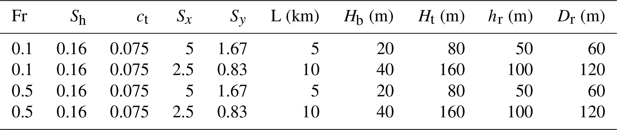
The investigation of flow over the hill provided a baseline for simulating AGWs under linearly stratified free atmospheric conditions. This was then extended to the wind farm canopy (WFC). Simulation sets 2 and 3 from Table 3 are re-run, this time with the wind farm canopy. The setups are the same as those of the hill cases described in Sect. 5.1.5 and 5.1.6, except that the hill is replaced with a wind farm canopy, where the canopy length and height correspond to the hill's half width at half height and maximum height, respectively. The parameters used to model the wind farm canopy are given in Table 4. Similarly to the hill case, the slope parameter is kept constant, i.e., S_h=0.16, and two values of Fr, i.e., 0.1 and 0.5, are considered. The thickness of the wind farm layer (i.e., the rotor diameter), the hub height, and C_t are varied as c_t is kept constant, i.e., 0.075. As shown in Table 4, the WFC starts at H_b=20 m and goes to H_t=80 m vertically for L=5 km such that hub height is h_r=50 m and the rotor diameter is D_r=60 m. For L=10 km, H_b=40 m and H_t=160 m, with the wind farm layer being 120 m thick and hub height at 100 m. Therefore, the turbine thrust is stronger for the L=10 km cases than for the L=5 km cases because of higher hub height and a bigger rotor.

Table 4 Wind farm canopy parameters. Note that the canopy only extends over the rotor diameter, so the bottom of the canopy is at H_b, and the top is at H_t.

5.2.1 Impact of damping layer thickness

Figure 11 shows that the results for the canopy case are similar to those of the hill (Fig. 9) in terms of the sensitivity of the reflection coefficient of the damping layer thickness and damping coefficient for the two Fr cases. The main difference is that the reduction in Cr with damping layer thickness when Fr=0.1 is monotonic for the canopy case and does not show the variation seen for the hill. The reasons for this are explored in Sect. 5.2.2.

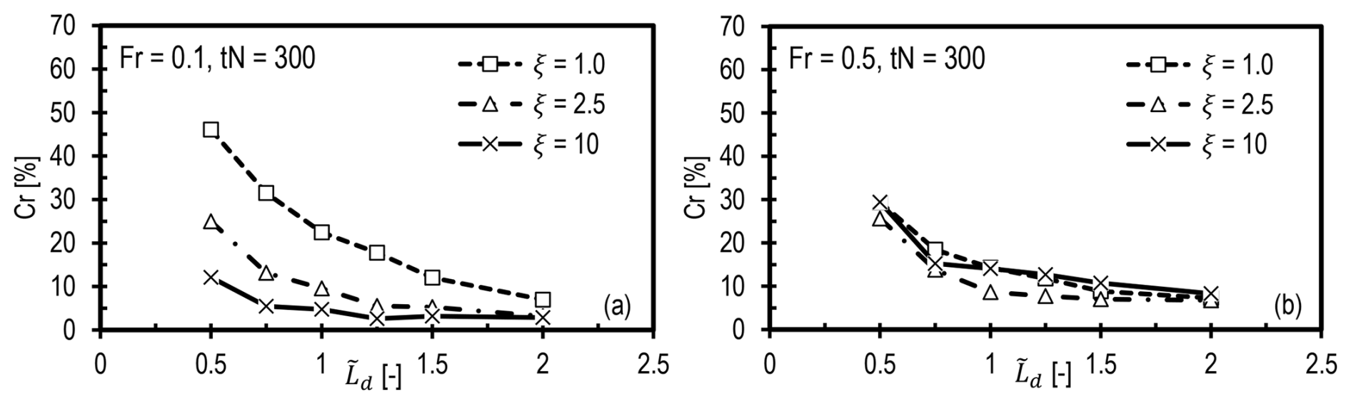
Figure 11 Reflection coefficient for the wind farm canopy case as a function of normalized damping layer thickness for different values of the damping coefficient when (a) Fr = 0.1 and (b) Fr=0.5.

Generally, thicker damping layers compensate for weaker damping coefficients. More importantly, for almost all values of ξ and ${\stackrel{\mathrm{̃}}{L}}_{\mathrm{d}}<\mathrm{1}$, Cr exceeds the threshold selected in this study for an acceptable level of reflection. Figure 11a shows that the suitable damping coefficient range for Fr=0.1 is still 1.0 to 10, with 10 being optimal for all damping layer thicknesses. Likewise, Fig. 11b shows that ξ=2.5 is the optimal damping coefficient for Fr=0.5, for all damping layer thicknesses. Furthermore, values of ξ=1 and 10 appear to be slightly less effective in damping reflections than a value of ξ=2.5.

5.2.2 Impact of domain size

The domain length is normalized based on the horizontal wavelength predicted from the linear theory for a hill using the wind farm canopy height and length instead of the hill maximum height and half width at half height, respectively. We calculate the effective wavelengths from the simulations at tN=300 to compare with the predicted wavelengths, where the horizontal wavelength is calculated based on a horizontal slice at ${\stackrel{\mathrm{̃}}{L}}_z=\mathrm{1.0}$ through the flow fields shown in Fig. 12 and the vertical wavelength is similarly calculated based on a vertical slice at X=0. In general, the calculated wavelengths match the predicted wavelengths.

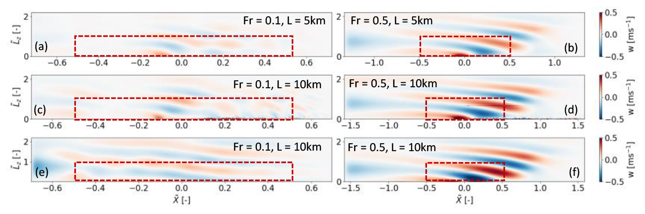
Figure 12 Plots (a)–(d) show vertical velocity of flow through and around the wind farm canopy with lengths L=5 and 10 km for Fr=0.1 and 0.5 and $\stackrel{\mathrm{̃}}{X}=\mathrm{1.0}$. For comparison, the plots (e)–(f) show the corresponding hill cases, where L=10 km for Fr=0.1 and 0.5 and $\stackrel{\mathrm{̃}}{X}=\mathrm{1.0}$. The region inside the dashed red box is the non-damped domain.

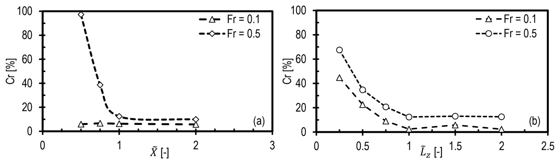
Figure 13 Reflection coefficient for the wind farm canopy case as a function of (a) domain length for Fr=0.1 and Fr=0.5 and (b) domain height for Fr=0.1, ${\stackrel{\mathrm{̃}}{L}}_{\mathrm{d}}=\mathrm{1.5}$ and Fr=0.5, ${\stackrel{\mathrm{̃}}{L}}_{\mathrm{d}}=\mathrm{1.2}$.

It is interesting to note that the wave shape for the canopy is significantly different from that of the hill for the same conditions and optimal simulation setup. The vertical velocity fields for the two wind farm canopy lengths and one hill half width (i.e., L=10 km) are shown in Fig. 12. For the WFC, there are two prominent wave trains for the Fr=0.1 cases shown in Fig. 12a and c, one at the entrance and the other at the canopy exit. The most dominant wave train is caused by upward flow deflection at the entrance due to the thrust force at the start of the canopy. The wave at the canopy exit results from the downward flow as the thrust force abruptly ends. These waves are out of phase and propagate at the same angle to the horizontal, and their interaction leads to a distorted wave spectrum. Therefore, the effective wavelength from a canopy simulation differs from that predicted if the most dominant wave train is considered, though the wavelength calculated using the global maxima at the canopy entrance and global minima at the canopy exit does provide a good match. This difference in wave shapes for the WFC and the hill case can be seen by comparing the plots in Fig. 12a and c with those in e. When referring to the monotonic Cr plots in Fig. 11a and nearly constant values in Fig. 13a for Fr=0.1, it seems that the dominant wave train triggered by canopy entrance is more critical in terms of simulation setup. For this case, the dominant wave train propagates out, both upstream and downstream. The second, smaller wave train at the exit propagates similarly, merging with the first to give the patterns seen in the plots in Fig. 12a and c. For Fr=0.5, we see only one wave train in the plots in Fig. 12b and d because the advection speeds in this case, 25 and 50 m s⁻¹, for the 10 km canopy and the 5 km canopy, respectively, are higher than the wave speed in this case. These advection speeds are higher than those generally observed for a wind farm but are used here to fix the value of Fr=0.5 for practical values of N when L is a constraint. As can be seen in the plots in Fig. 12b, d, and f, the wave shape and wavelengths are the same for the WFC and hill cases when Fr=0.5; however, the amplitude of the vertical velocity is higher in the hill case.

Another important observation is the increased wave energy accumulation at the inlet in all cases compared with the hill simulations, suggesting that Dirichlet inflow boundary conditions are inappropriate when simulating AGWs. In contrast to the zero-gradient outflow boundary condition, which appears to advect the waves through the outlet, the inflow boundary condition is not influenced by any approaching waves (i.e., the prescribed boundary values remain as prescribed and are not perturbed by the gravity waves). Thus, the user-prescribed inflow velocity is not truly representative of a flow regime where AGWs are present. As a consequence, wave energy accumulates at the inlet, and the inlet RDL can only delay its propagation back into the domain. Further work concerning how to effectively contain or eliminate this energy accumulation at the inlet is required.

In terms of the main aim of this study, the waves are effectively damped, especially in the top and outlet RDLs, suggesting that the optimal setups from the hill case are also optimal for the wind farm canopy. Figure 13a shows that there is no impact of the domain length on Cr when Fr=0.1. This is because the domain lengths were set as a function of λ_hor predicted from the linear theory, which is significantly greater than the wavelength of the dominant wave train at the entrance of the canopy. When Fr=0.5, similar behavior is seen to that in the hill case, where Cr reduces with increasing domain length and is minimum when $\stackrel{\mathrm{̃}}{X}>\mathrm{1.0}$. However, Cr values remain higher than 10 % because of faster energy accumulation for higher advection speeds than observed wind speeds for a wind farm.

The impact of domain height on the reflections is also the same as that of the hill case. As shown in Fig. 13b, Cr is minimized for domain heights greater than λ_ver. It is important to recall that vertical wavelength depends on $U/N$, which holds true for both the canopy case and the hill case. The value of Cr is higher when Fr=0.5 because of high amplitudes due to a high advection speed, i.e., 25 m s⁻¹. Based on these observations, we suggest setting the domain length and height in wind farm simulations to at least one predicted effective horizontal and vertical wavelength, respectively. However, the link between high inflow velocities, wave amplitudes and wave trains should be investigated by modeling wind farms with actuator models for a more accurate representation of wind farm flow dynamics.

6 Conclusions

This study aims to provide guidelines for atmospheric flow simulations that include atmospheric gravity waves by relating key physical and simulation parameters. The study is first carried out for a 2D hill in stably stratified flow to compare the results to those of an analytical solution. The findings are then tested for flow through wind farms, approximated with a wind farm canopy model. Based on recent findings in the literature, only Rayleigh damping gravity wave treatment was investigated. Therefore, the findings apply to simulation setups with Rayleigh damping layers and inflow–outflow boundary conditions solved with finite-volume codes.

Simulation time is one of the most critical parameters in simulations, including gravity waves. In all cases, a longer simulation time resulted in the accumulation of wave energy at the inlet boundary, and the reflections gradually became stronger. Thus, we conclude that the Rayleigh damping method attenuates gravity waves to an extent that may not work for a long simulation, such as a diurnal simulation. Therefore, a robust technique is required to handle both the energy accumulation and the reflections. In terms of time-step size and grid resolution, the typical values used in wind farm LES (i.e., $\mathrm{0.5}<t<\mathrm{1.0}$ and $\mathrm{5}<\mathrm{\Delta }x,\mathrm{\Delta }y,\mathrm{\Delta }z<\mathrm{20}$) are more than sufficient to resolve the AGWs. Thus, the simulation setups used for the investigated Fr range are independent of the time-step size and grid resolution because the time periods and wavelengths of AGWs are several times bigger.

The results regarding the configuration of the damping layers show a trade-off between the ability to correctly resolve gravity waves and computational resources. With periodic conditions in the lateral direction, the highest accuracy can be achieved with damping layers of a thickness exceeding the effective vertical wavelength at the inlet, top, and outlet. In the case of limitations on computational resources, a combination of damping layers of the same thickness at the inlet and top could still be reasonable.

Our test shows that for various Froude numbers, small damping coefficients would not be effective, even for damping thickness 2 to 5 times greater than the effective vertical wavelength. Likewise, the reflections are higher for layers with excessively large damping coefficients and might distort the solution in regions of the non-damped domain close to the damping layer. The most suitable damping coefficients are values from 1 to 10 when the damping coefficient is normalized with the Brunt–Väisälä frequency. The thickness of the damping layer should be at least one effective vertical wavelength, and thicknesses exceeding 1.5 times the effective vertical wavelength may be unnecessary. The wave direction is critical to understanding AGWs, but it should not affect the wave damping as it is applied to velocity components; usually, the vertical velocity is set to zero, and the other two are set to the geostrophic components.

The domain length should be scaled with the effective horizontal wavelength and not with the length of the hill or wind farm. The reflection coefficient as a function of domain length, normalized by effective horizontal wavelength, shows that large domains are more effective at avoiding undesirable levels of reflections from the domain boundaries. For domain lengths exceeding one horizontal wavelength, the reflection of the upward-propagating energy is less than 6 % in the hill case. The reflection coefficient was slightly higher for the wind farm canopy cases due to the interaction of the wave trains at the canopy entrance and exit. Therefore, further investigation using, for example, an actuator disk approach to model wind turbines is required to thoroughly test the optimal setups and understand the wave dynamics. For both flow scenarios, i.e., the hill case and the canopy case, increasing the domain length beyond λ_hor shows a small reduction in the reflection coefficient. A similar impact on the reflection coefficient is observed when varying the non-damped domain height, and setting it to at least one effective vertical wavelength is recommended. It is important to point out that the wave reflection coefficient in this study was calculated by taking the ratio of energy values. This can be misleading in some cases, as the reflected waves can be directed upward, thus reducing the Cr value. Visual inspection of the vertical velocity fields is recommended to cross-check the Cr values.

These recommendations are based on linearly stratified atmospheric flows. Aspects like turbulence and a more realistic and complex temperature structure of the atmosphere are not considered in this study. Nevertheless, this work should help provide useful guidelines for setting up simulations that include atmospheric gravity waves in wind energy applications. We have tested these findings with another finite-volume code, TOSCA (Stipa et al., 2024), and found results consistent with those of SOWFA.

In further work (Khan et al., 2024), the impact of the inversion layer (inversion Froude number and height) on the setup is explored, as well as the impact of turbulence and the Coriolis force. In extending the current study, we validated the findings mentioned above for conventionally neutral boundary layer conditions. An additional observation of the follow-up study is that the Rayleigh damping layer along with the advection damping layer (as detailed in Lanzilao and Meyers, 2023) is better at containing energy accumulation at the inlet than using the Rayleigh damping layer alone. More importantly, the study is intended to develop an inflow boundary condition that can avoid energy accumulation at the inlet based on an inflow which accounts for the presence of AGWs.

Appendix A: Configuration of damping layers

The reflection of waves from the top boundary is expected, as the typically used boundary conditions to model an arbitrary location in the atmosphere are mostly fully reflective. Since gravity waves travel vertically, one would anticipate reflections from the top boundary if forcing zones are not used there. Intriguingly, with inflow–outflow boundary conditions, the damping layers are needed at other boundaries, too. For instance, the reflected waves from the top are directed toward the outlet, and weak reflections may also appear there. Likewise, the wave energy distributes throughout the domain and accumulates over time if not damped at the boundaries. This is evident as reflections from the inlet propagate into the domain after one to two flow-through times. Thus, damping the waves at various boundaries is necessary for realistic simulations. Sometimes, the solution for a setup without an appropriate damping layer configuration will diverge due to numerical instability caused by excessive flow velocity from complex reflected wave interactions.

In this context, deciding on the configuration of damping layers becomes important when setting up simulations involving gravity waves. We explored the configuration of damping layers to come up with a base case. The test cases and normalized errors are shown in Fig. A1.

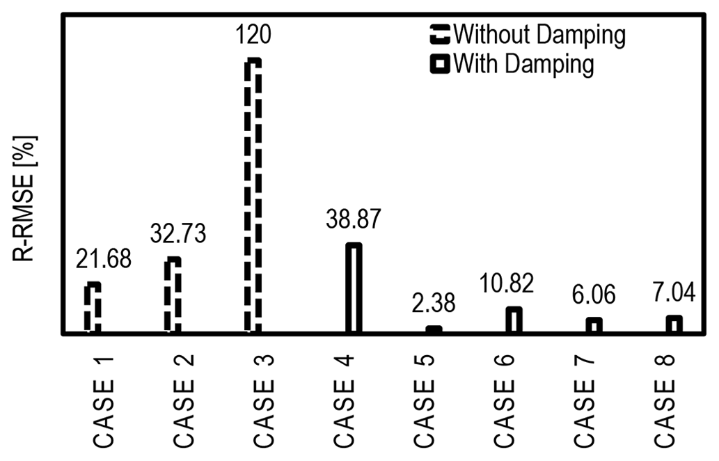
Figure A1 Comparison of R-RMSE for various damping configurations designed to acquire the most suitable arrangement for the base case.

At this point, it is important to highlight that the minimum amount of reflections is the user's choice. Since the reflections intensify over the simulation time, it may be the case that a user will opt for a configuration based on the availability of computational resources and the simulation time of their interest. Thus, a simulation without any forcing zones is the first possibility. The domain height is critical when there is no damping. This can be established by comparing Cases 1, 2, and 3, where the domain height (L_z) is 1, 2, and 3 times the effective vertical wavelength, respectively. Reflections increase rapidly when increasing the domain height, from 22 % to 33 % and 120 % in Cases 1 to 3, respectively. However, none of these cases fall below the criterion for an acceptable amount of reflection. Thus, we opt to use Rayleigh damping, and it is evident that only having a top Rayleigh-damped layer (Case 4) is insufficient to reduce reflections to an acceptable level. The R-RMSE for this case is 39 %, and the solution for the hill case is contaminated by reflections from the inlet such that the actual gravity waves disappear entirely. This suggests that it is better not to have a damping layer rather than only having a damping layer at the top and instead have a setup with a domain height just over one effective vertical wavelength. This would be viable only when a maximum value of R-RMSE or Cr of about 20 % is an acceptable criterion for a given problem.

The most suitable setup is to have damping layers at the inlet, outlet, and top with the same damping characteristics. This is Case 5 in Fig. A1, where the R-RMSE is only 2.38 %. If the damping layer thickness is reduced by half while having damping on all three sides (Case 6), the R-RMSE increases to 10 %. Case 7, featuring a combination of damping layers at the top and outlet, appears to be better than Case 6, as here the R-RMSE is 6 %. Damping at the top and inlet (Case 8) is slightly more reflective (R-RMSE 7 %) than in Case 7. There can be other possible configurations, but this analysis gives enough insight to decide on a suitable configuration for a sufficiently accurate base case. Altogether, the configuration of damping layers is a trade-off between computational resources and the desired accuracy of the solution, which depends on the user's choice regarding the acceptable degree of reflection.