Source–load matching and energy storage optimization strategies for regional wind–solar energy systems

In response to the issue of limited new energy output leading to poor smoothing effects on grid-connected load fluctuations, this paper proposes a load-power smoothing method based on “one source with multiple loads”. The method comprehensively considers the proximity between the source and the load, as well as the correlation between their power fluctuations, using these factors as evaluation criteria for source-side and load-side matching in regional power grids. Initially, loads are clustered and divided based on power frequency division. The EEMD algorithm is then applied to obtain wind and solar energy outputs with greater complementarity and smoother fluctuations, leveraging their low-frequency correlation. Subsequently, a load-tracking coefficient is used to compare the matching degree between wind–solar power output and different loads, selecting the most compatible load and output for source–load matching and smoothing. Concurrently, a gray-wolf-optimization (GWO) algorithm based on Tent chaotic mapping is employed to optimize edge energy storage at different load sides, minimizing overall grid-connected load-power fluctuations. Numerical results demonstrate that the proposed method can fully utilize the stable output from the low-frequency correlation of wind and solar energy, combined with energy storage, to significantly reduce the fluctuation rate of regional grid-connected loads. This effectively promotes local absorption of source loads, thereby alleviating the pressure on the grid side caused by the randomness and volatility on both sides of the source load.

1 Introduction

In response to China's dual carbon goals, new power systems utilizing renewable energy sources like wind and photovoltaic are rapidly advancing. The installed capacity of wind turbines and photovoltaic units, crucial components of renewable energy, is growing (Xi, 2020; Gao, 2022). However, both wind and photovoltaic power generation are highly volatile and stochastic, leading to increased pressure on grid-side dispatch when parallelized with traditional load demands (Qu and Ye, 2023; Lee and Baldick, 2017; Ma et al., 2020; Oh and Son, 2022; Li et al., 2022). Often, the installed capacity of wind–solar units in a region is insufficient to meet local load demands, or their utilization is limited, resulting in low-efficiency suppression of load fluctuations.

Despite these challenges, the consistency of regional source–load fluctuations can be leveraged to improve local consumption of wind–solar power and reduce grid-side pressure from load-power fluctuations, which is crucial for regional grid-connected dispatch. One effective strategy is the use of wind–solar correlation for regional power suppression, which has been extensively studied (Liang et al., 2023; Hu et al., 2024; Xie et al., 2017; Tan et al., 2022; Dong et al., 2018; Haensch et al., 2024; Wang et al., 2020; Zhao et al., 2020). By considering the complementary characteristics of wind and solar power, volatility and randomness in the original output can be reduced. For instance, typical wind–solar output scenarios can be generated based on wind–solar correlation, aiding in optimal scheduling for microgrids.

The traditional energy optimization dispatching strategy is distinct from the source–load matching strategy, which focuses on regional renewable energy consumption and grid-connected power fluctuation reduction. Source–load matching is implemented based on evaluating the load-tracking degree, which considers the smoothness of the load tracking and residual load curve (Zhu et al., 2024). To enhance load tracking, different tracking coefficient models are established based on the overall system fluctuation's smoothness (Shi et al., 2023; Mitrofanov and Baykasenov, 2022; Beluco et al., 2008). Additionally, the Copula function can evaluate source–load matching, inverting the energy side's complementary characteristics (Ren et al., 2024). However, these methods are often limited to considering power differences or fluctuation similarities between the source and load, or they only address matching between single power and load sides.

In this paper, we propose a source–load matching strategy based on wind–solar complementarity and the “one source with multiple loads” concept. We prioritize the more stable low-frequency wind–solar output to match load-power fluctuations according to load-tracking criteria. We also optimize the edge storage charging and discharging strategy for each load group using the gray-wolf-optimization (GWO) algorithm with Tent chaotic mapping, aiming to minimize overall load fluctuation in regional grid connections and reduce power fluctuations on both sides of the grid.

Unlike current research on microgrid or regional source–load matching models, which typically consider a single power side and a single load group, this paper delves deeper into the impact of different power-side suppression abilities on various load groups, influencing regional grid fluctuations. We construct a “one source with multiple loads” regional grid framework, utilizing a typical wind–solar cogeneration plant and multiple load groups with edge storage. K-medoid clustering is used to categorize loads into groups with typical energy use characteristics. Based on the complementary low-frequency correlation of wind–solar power, the source-side power output is smoothed. The proposed load-tracking index is then employed to track load–side power fluctuations, reducing regional grid-connected power fluctuations.

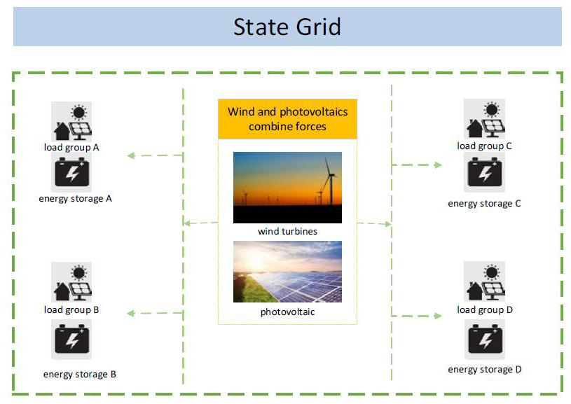
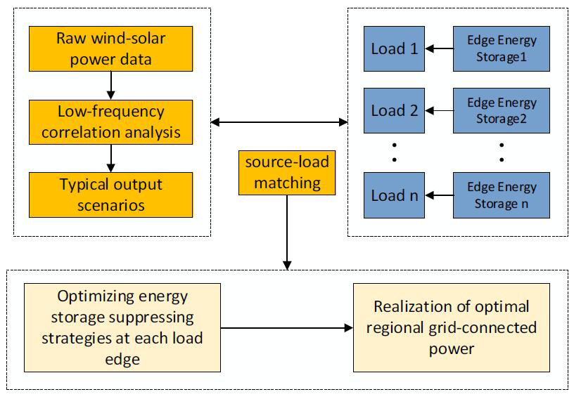
The framework of “the one source with many loads” regional grid is shown in Fig. 1.

The primary contributions of this paper are as follows:

• Frequency decomposition of the daily wind–solar output, correlation analysis of the decomposed low-frequency components and generation of a daily scenario set of wind–solar low-frequency output are performed. Euclidean distance is then used to compare each scenario to the original output of the corresponding day, and the closest day is selected as a replacement of the output of that day.

• The load is clustered based on the rough K-means of variational firefly optimization. The load-tracking evaluation criteria proposed in this paper are used to compare the matching degree between the output scenario and each load group. The load group with the highest source–load matching degree is selected as the output satisfaction object for that day.

• The gray-wolf-optimization algorithm based on Tent chaotic mapping is used to optimize each load–side edge energy storage leveling strategy to minimize the fluctuation of regional grid-connected load, promote the level of wind–solar consumption and reduce the pressure of grid-side dispatch.

Figure 1 “One source with multiple loads” regional power grid framework.

The specific steps of power leveling are shown in Fig. 2.

Figure 2 Flow chart of regional source–load matching and stabilizing method.

2 Source–load matching for regional wind–solar systems

2.1 CEEMD-based wind–solar output frequency decomposition

In this paper, based on a previous study (Mahdavi et al., 2023), we further study the smoothing effect of the source-side power output on the load-side fluctuation. Based on not changing the capacity configuration in the original region, the obtained typical daily scenario set of wind–solar power output and the load scenario are source–load-matched to achieve the power fluctuation smoothing at the regional grid connection.

To better achieve the decomposition effect, this paper adopts the CEEMD (complementary ensemble empirical mode decomposition) algorithm to decompose the frequency of the original wind–solar output data. CEEMD has the characteristics of independent and homogeneously distributed addition of white noise with opposite signs to the original signal for auxiliary decomposition. It can compensate for the shortcomings of modal mixing in the traditional empirical mode decomposition (EMD) while better reducing the noise remaining in the original signal and decomposition errors (Liu et al., 2024). The specific decomposition steps are as follows.

1. Add a pair of random Gaussian white noise values – one positive and one negative – to the original sequence as follows:

   $$\begin{array}{}\text{(1)}& {\displaystyle }{X}^{+}\left(t\right)=x\left(t\right)+{\mathit{\mu }}^{+}\left(t\right)\text{(2)}& {\displaystyle }{X}^{-}\left(t\right)=x\left(t\right)+{\mathit{\mu }}^{-}\left(t\right),\end{array}$$

   where X⁺(t) and X⁻(t) are the sequences after adding positive and negative random Gaussian white noise, respectively, and μ⁺(t) and μ⁻(t) represent the positive and negative Gaussian white noise components, respectively.

2. Use the EMD decomposition of the newly generated signal to obtain the intrinsic mode function (IMF) components of each order:

   $$\begin{array}{}\text{(3)}& {\displaystyle }{X}^{+}\left(t\right)=\sum _{i=\mathrm{1}}^m{c}_i^{+}\left(t\right)+r^{+}\left(t\right)\text{(4)}& {\displaystyle }{X}^{-}\left(t\right)=\sum _{i=\mathrm{1}}^m{c}_i^{-}\left(t\right)+r^{-}\left(t\right),\end{array}$$

   where $c_i^{+}\left(t\right)$ and $c_i^{-}\left(t\right)$ are the ith IMF components of the decomposition, and r⁺(t) and r⁻(t) are the remaining terms of the decomposition.

3. Repeat the above steps n times. Each repetition adds a new and different sequence of paired Gaussian white noise.

4. Sum up the IMF components obtained from each repetition to take the mean value as the final decomposition result. The final c_i(t) and r(t) are expressed as follows:

   $$\begin{array}{}\text{(5)}& {\displaystyle }{c}_i\left(t\right)={\displaystyle \frac{\mathrm{1}}{\mathrm{2}n}}\sum _{i=\mathrm{1}}^n\left(c_{ji}^{+}\right(t)+c_{ji}^{-}(t\left)\right)\text{(6)}& {\displaystyle }r\left(t\right)={\displaystyle \frac{\mathrm{1}}{n}}\sum _{i=\mathrm{1}}^n\left(r_j^{+}\right(t)+r_j^{-}(t\left)\right),\end{array}$$

   where $c_{ji}^{+}\left(t\right)$ and $c_{ji}^{-}\left(t\right)$ are the ith IMF components obtained from the decomposition at the jth repetition, $r_j^{+}\left(t\right)$ and $r_j^{-}\left(t\right)$ are the residuals obtained from the decomposition at the jth repetition, c_i(t) is the ith IMF component from the final decomposition, and r(t) is the remaining amount of final decomposition.

2.2 Rough-load clustering optimized by the mutation firefly algorithm

This paper uses a variational strategy and a firefly algorithm with differential evolution to optimize the traditional clustering algorithm (Wei et al., 2023). The rough K-means algorithm is an improvement of the classical K-means algorithm, and the difference is that the algorithm divides the sample objects that cannot be determined into the boundary set of the class. The division is based on the presence or absence of other clustering centers with a difference between the distance and the minimum distance from the sample object being less than a given threshold.

The core concepts of rough set theory are upper approximation and lower approximation rather than boundary domain. The variation in the number of objects in the lower approximation and boundary set, along with the variability in object distribution, dynamically adjusts the center-of-mass weights. The relative distance is

$$\begin{array}{}\text{(7)}& T^{\prime }=\left\{t:{\displaystyle \frac{\mathrm{d}\left(x_n,m_k\right)}{\mathrm{d}\left(x_n,m_h\right)}}\le \mathit{\xi }\wedge h\ne k\right\}.\end{array}$$

The variant firefly optimization algorithm makes full use of the information of individual firefly populations through a double-variant strategy, which significantly improves the ability of the algorithm to jump out of the local optimum and converge to the global optimum with probability one, given a large-enough number of iterations. The new objective function value is constructed as the firefly light intensity for the initial clustering centroid search, and the optimal solution found by the firefly algorithm is used as the clustering center of the algorithm for clustering iterations:

$$\begin{array}{}\text{(8)}& I=f\left(x\right)={\left({\displaystyle \frac{O}{I}}\right)}^{\mathit{\lambda }},\end{array}$$

where I is the intraclass distance, which is the sum of the distances from each data sample in each class to its cluster center, and O is the interclass distance, which is the distance between the cluster centers. When λ≥1, the data may be out of range if the number of samples and the number of dimensional bases are large, and $\mathit{\lambda }=\mathrm{1}/\mathrm{2}$ is taken in this study.

2.3 Load-tracking evaluation criteria

This paper considers the proximity of source–load power-magnitude and the correlation degree of source–load-power fluctuation as evaluation criteria of source-side load tracking. Based on the fact that Spearman's coefficient and Euclidean distance present complementary advantages and disadvantages, in order to measure correlation, Euclidean distance and rank correlation coefficient are used to calculate them, respectively. The equation is shown in the following way:

$$\begin{array}{}\text{(9)}& max{\mathit{\theta }}^i={\mathit{\alpha }}_{\mathrm{1}}{\mathit{\delta }}_{\mathrm{1}}^i+{\mathit{\alpha }}_{\mathrm{2}}{\mathit{\delta }}_{\mathrm{2}}^i,\end{array}$$

where θⁱ is the match between the source-side output and the ith load group; ${\mathit{\delta }}_{\mathrm{1}}^i$ is the tracking coefficient between the source-side output and the ith load group; ${\mathit{\delta }}_{\mathrm{2}}^i$ is the correlation between the normalized source-side output and the ith load group; α₁ and α₂ are the weight coefficients of the corresponding indicators; and the initial ratio of the two is selected as 1 : 1 in this paper, considering their different effects on the matching degree.

$$\begin{array}{}\text{(10)}& {\displaystyle }{\mathit{\lambda }}^i=\sqrt{\sum _{t=\mathrm{1}}^T(P^t-L_i^t{)}^{\mathrm{2}}}\text{(11)}& {\displaystyle }{\mathit{\xi }}_{\mathrm{1}}^i={\displaystyle \frac{{\mathit{\lambda }}^i}{\sum _{n=\mathrm{1}}^N{\mathit{\lambda }}^n}},\end{array}$$

where P^t and $L_i^t$ are the output power and the load power of the ith load group at moment t, respectively; T is the number of moments of that day (T=24); and λⁱ and λⁿ are the Euclidean distances between the source-side output and the power of the ith and nth load groups, respectively, for that day. N is the total number of load groups. ${\mathit{\xi }}_{\mathrm{1}}^i$ is the Euclidean distance between the normalized source-side output and the ith load group.

$$\begin{array}{}\text{(12)}& {\mathit{\delta }}_{\mathrm{1}}^i=\mathrm{1}-{\mathit{\xi }}_{\mathrm{1}}^i\end{array}$$

Spearman rank correlation coefficient was used to do a correlation analysis between wind–solar low-frequency output and each load power. Spearman correlation coefficient is a nonparametric statistical method of rank correlation using monotonic equations in statistics to evaluate the correlation between two statistical variables. The basic idea is that there are three binary distributions of random vectors $\left(m_{\mathrm{1}},n_{\mathrm{1}}\right),\left(m_{\mathrm{2}},n_{\mathrm{2}}\right)$ and (m₃,n₃) with the difference between the probability that at least one of them occurs in concert with the other distributions and the probability that at least one of them does not occur in concert with the other distributions as the correlation indicator describing the random variables (Wei et al., 2023), which is calculated as the following equation:

$$\begin{array}{}\text{(13)}& \mathit{\tau }=\mathrm{1}-[\mathrm{6}\sum _{t=\mathrm{1}}^T{d}_t^{\mathrm{2}}/T(T^{\mathrm{2}}-\mathrm{1}\left)\right],\end{array}$$

where τ is the Spearman correlation coefficient between any two vectors; T is the vector dimension, which in this paper is the 24 time periods that divide each day in source–load matching; and d is the set of element-ranking differences in the two vectors.

$$\begin{array}{}\text{(14)}& {\mathit{\delta }}_{\mathrm{2}}^i={\displaystyle \frac{{\mathit{\tau }}^i}{\sum _{n=\mathrm{1}}^N{\mathit{\tau }}^n}}\end{array}$$

To make a uniform distance and a correlation–variation relationship, Eq. (14) normalizes Spearman coefficients to [0, 1], ensuring compatibility with Euclidean distance, where τⁱ and τⁿ are the correlation coefficients between the source-side output and the ith and nth load groups, respectively, for that day, and N is the number of load groups.

According to the above load-tracking evaluation criteria, the matching degree between the wind–solar system's low-frequency output and each load's power is compared, and the most matching load is selected as the target of the power leveling on that day. The wind–solar excess energy is used to charge the energy storage corresponding to the matched load. When the load is not matched with the energy output on a given day and the load has too much fluctuation, the energy storage – according to its own SOC state and the set fluctuation threshold – smooths the load to a certain extent. If the wind–solar output has excess energy in a specific period, that energy is used to charge the energy storage. This ensures that on days when the load and output do not match, the energy storage can operate within a specific scheduling interval, using renewable resources, reducing pressure on the grid, and calming down load fluctuation, while avoiding the waste of energy when the wind–solar power is connected to the grid (Luo et al., 2021).

3 Load–edge energy storage suppressing strategy

In order to better achieve the overall grid-connected power fluctuation smoothing of regional loads, the charging and discharging strategies of small-capacity energy storage on each load group side are optimized using the gray wolf algorithm based on Tent chaotic mapping to minimize the overall fluctuation rate of regional loads. The method proposed in this paper, compared with the traditional energy storage methods, can optimize the single-period load reduction to a more detailed multi-time-period reduction. This helps avoid dispatch pressure on the grid after a substantial load smoothing, which can occur after the load rises again during peak and valley periods, to achieve the reduction of the overall fluctuation rate.

3.1 Gray-wolf-optimization algorithm based on Tent chaotic mapping

Compared with the traditional particle swarm algorithm and genetic algorithm, the gray wolf algorithm has a good performance in terms of the accuracy of solving problems and calculating convergence speeds due to its strong convergence performance, simple structure, few parameters to be adjusted, and the ability to achieve a balance between local optimization and global search (Wei et al., 2023). This paper uses the improved gray-wolf-optimization algorithm with Tent chaotic mapping to flatten the marginal energy storage on different load sides.

The core idea of the gray wolf algorithm is to mathematically model the social hierarchy of gray wolves using GWO by defining the first-, second- and third-best wolves (optimal solutions) as α, β and δ, respectively, and using those wolves to guide the other wolves in their search toward the goal. The remaining wolves (candidate solutions) are defined as ω, and they update their position around α, β and δ.

Chaos uses randomness, traversal and initial value sensitivity to speed up the convergence of the algorithm, generating chaotic sequences based on Tent mapping to initialize the population:

$$\begin{array}{}\text{(15)}& Z_{I+\mathrm{1}}^k=\left\{\begin{array}{ll}\frac{Z_I^k}{u},& \mathrm{0}\le Z_I^k\le u\\ \frac{\mathrm{1}-Z_I^k}{\mathrm{1}-u},& u<Z_I^k\le \mathrm{1}\end{array}\right.,\end{array}$$

where k is the number of populations, I is the number of current iterations and u (to maintain the randomness of the initialization information of the algorithm) takes the value of $u\subset \text{rand}(\mathrm{0},\mathrm{1})$. Combined with the chaotic sequence $Z_I^k$, the further process of generating the sequence $X_I^k$ of initial locations of individual gray wolves in the search area is as follows:

$$\begin{array}{}\text{(16)}& X_I^k=X_{I,min}^k+Z_I^k\left(X_{I,max}^k-X_{I,min}^k\right),\end{array}$$

where $X_{I,\max }^k$ and $X_{I,\min }^k$ are the maximum and minimum value of $X_I^k$, respectively.

A dynamic weight factor b, which changes in a linearly decreasing manner, is introduced to update the gray-wolf-individual step size dynamically:

$$\begin{array}{}\text{(17)}& b\left(I\right)=b_{\mathrm{f}}-{\displaystyle \frac{I}{\text{maxiter}}}\left(b_{\mathrm{f}}-b_{\mathrm{s}}\right),\end{array}$$

where maxiter denotes maximum iterations and b_s and b_f denote the initial and final values of the weighting factors, respectively.

A fitness scaling factor was introduced to dynamically weight the averages and differentiate the contributions of the head wolves, thus effectively differentiating the different guiding roles of head wolves α, β and δ in subsequent position updates of each gray wolf:

$$\begin{array}{}\text{(18)}& \left\{\begin{array}{l}f=\left|f_{\mathit{\alpha }}+f_{\mathit{\beta }}+f_{\mathit{\delta }}\right|\\ v_{\mathrm{1}}=\frac{f_{\mathit{\alpha }}}{f},v_{\mathrm{2}}=\frac{f_{\mathit{\beta }}}{f},v_{\mathrm{3}}=\frac{f_{\mathit{\delta }}}{f},f>\mathrm{0}\\ v_{\mathrm{1}}=v_{\mathrm{2}}=v_{\mathrm{3}}=\frac{\mathrm{1}}{\mathrm{3}},f=\mathrm{0}\end{array}\right.,\end{array}$$

where v₁, v₂ and v₃ are the adaptation scale factors, and f_α, f_β and f_δ are the adaptation values of α, β and δ, respectively.

The fused improved position update formula is as follows:

$$\begin{array}{}\text{(19)}& X\left(I+\mathrm{1}\right)=b\left(I\right)\cdot r_{\mathrm{4}}\cdot \left(v_{\mathrm{1}}\cdot X_{\mathrm{1}}+v_{\mathrm{2}}\cdot X_{\mathrm{2}}+v_{\mathrm{3}}\cdot X_{\mathrm{3}}\right),\end{array}$$

where r₄ is a random vector between [0, 1].

3.2 Edge energy storage optimization model

The gray-wolf-optimization algorithm based on Tent chaotic mapping is used to optimize the charging and discharging power of the edge energy storage of the remaining load groups with the objective of minimizing the fluctuation of the regional required grid-leveling load to achieve the reduction of the regionally grid-connected load fluctuation. The optimization objective function is as follows:

$$\begin{array}{}\text{(20)}& min{F}_i=\left(\sum _{t=\mathrm{1}}^T{\displaystyle \frac{M_i(t+\mathrm{1})-M_i\left(t\right)}{M_i^{max}}}\right)/\mathrm{24},\end{array}$$

where F_i is the overall regional load fluctuation rate on day i, M_i is the overall regional load power on day i after source–load matching, $M_i^{\max }$ is the maximum load value on that day and T is the number of moments on that day (T=24).

The constraints are as follows:

1. wind farm operation

   $$\begin{array}{}\text{(21)}& \mathrm{0}\le P_{\mathrm{wind},\mathrm{s},\mathrm{t}}\le P_{\mathrm{wind},\mathrm{s},\mathrm{t}}^{max};\end{array}$$

2. photovoltaic plant operation

   $$\begin{array}{}\text{(22)}& \mathrm{0}\le P_{\mathrm{PV},\mathrm{s},\mathrm{t}}\le P_{\mathrm{PV},\mathrm{s},\mathrm{t}}^{max};\end{array}$$

3. load

   $$\begin{array}{}\text{(23)}& P_{\mathrm{LD},\mathrm{s},\mathrm{t}}^{min}\le P_{\mathrm{LD},\mathrm{s},\mathrm{t}}\le P_{\mathrm{LD},\mathrm{s},\mathrm{t}}^{max};\end{array}$$

4. energy storage (which includes the following energy-storage-specific constraints)

   charging and discharging power

   $$\begin{array}{}\text{(24)}& P_{\mathrm{ess},\mathrm{s},\mathrm{t}}^{min}\le P_{\mathrm{ess},\mathrm{s},\mathrm{t}}\le P_{\mathrm{ess},\mathrm{s},\mathrm{t}}^{max};\end{array}$$

   charge state

   $$\begin{array}{}\text{(25)}& {\text{SOC}}^{min}\le {\mathrm{SOC}}_{\mathrm{s},\mathrm{t}}\le {\text{SOC}}^{max};\end{array}$$

   discharge balance

   $$\begin{array}{}\text{(26)}& \sum _{t=\mathrm{1}}^T{P}_{\mathrm{ess}}\left(t\right)=\mathrm{0}.\end{array}$$

3.3 Energy-storage SOC control

The basic idea of energy storage leveling is as follows. On the day when the load matches the energy source, if the load is larger than the output and fluctuates widely, energy storage discharges to level the load. On the same day, if the load is smaller than the output, energy storage charges to avoid the waste of renewable energy. At the same time, on the day when the load does not match the energy output, if the load has a significant fluctuation, energy storage – according to its own SOC and the set fluctuation threshold – will level the load to a certain extent, in order to better protect the energy storage and prolong its lifespan.

In order to better protect the energy storage and prolong the life of the energy storage, it is necessary to limit the energy storage ground charge and discharge; i.e., the energy storage SOC is limited to [0.1, 0.9]. The SOC is calculated as follows:

discharging

$$\begin{array}{}\text{(27)}& S_{\mathrm{soc}}\left(t\right)=(\mathrm{1}-\mathit{\rho })S_{\mathrm{soc}}(t-\mathrm{1})-{\displaystyle \frac{P_{\mathrm{e}}\left(t\right)\mathrm{\Delta }t}{E{\mathit{\eta }}_{\mathrm{d}}}}\end{array}$$

charging

$$\begin{array}{}\text{(28)}& S_{\mathrm{soc}}\left(t\right)=(\mathrm{1}-\mathit{\rho })S_{\mathrm{soc}}(t-\mathrm{1})-{\displaystyle \frac{P_{\mathrm{e}}\left(t\right)\mathrm{\Delta }t{\mathit{\eta }}_{\mathrm{c}}}{E}},\end{array}$$

where S_soc(t) and S_soc(t−1) denote the SOC values of energy storage in period t and t−1, respectively; P_e(t) denotes the required leveling target of energy storage in period t; Δt is the length of the period; ρ is the self-discharge rate; η_d and η_c denote the energy storage discharge efficiency and charging efficiency, respectively; and E is the energy storage capacity.

4 Experiments and results

This paper analyzes the actual power output of a 100 MW wind farm and a 50 MW PV cogeneration farm and the actual loads of four typical load groups in the region in the summer of 2018 in a northwestern area.

From the scenario generation method described in the previous section, typical scenarios of wind and solar low-frequency output power are obtained, as shown in Fig. 3.

They are adopting the load-tracking evaluation criteria proposed in Sect. 2.3. Furthermore, combined with the local weather, the daily corresponding wind power and different load groups are matched and evaluated, and the load group with the highest degree of matching is selected as the main suppression target of the wind power on that day.

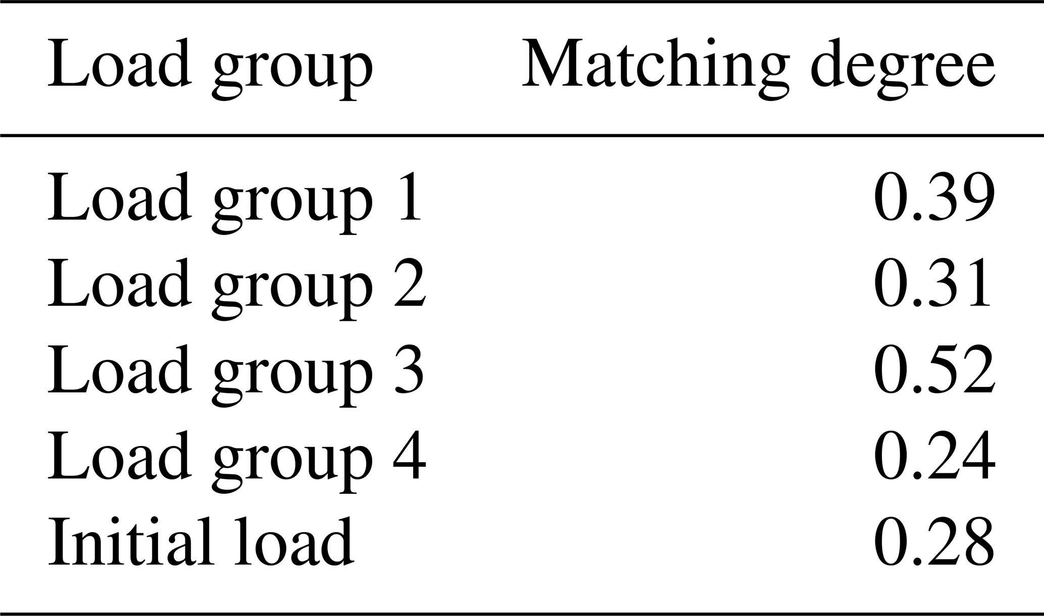
Table 1 shows the matching degree between source-side output and different load clusters and the original load for a particular day, where load cluster 5 is the original load before the clustering of loads. The table shows the matching degree between source-side output and original load to be less than 0.3, while the highest-matching degree of the clustered load groups can reach 0.52. Therefore, this paper can effectively explore the matching degree between source-side output and typical load groups after dividing the load clusters.

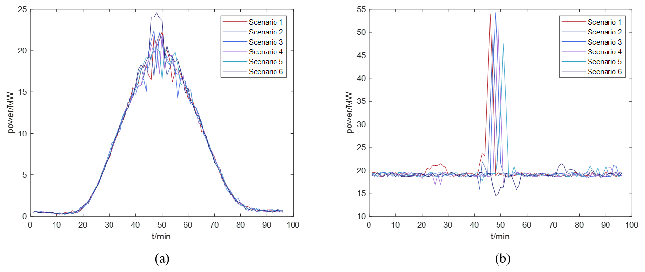
Figure 3 (a) Generation results of a wind power scenario. (b) Generation results of a PV scenario.

Table 1 Comparison of matching degrees on a certain day.

Figure 4 Source–load matching results.

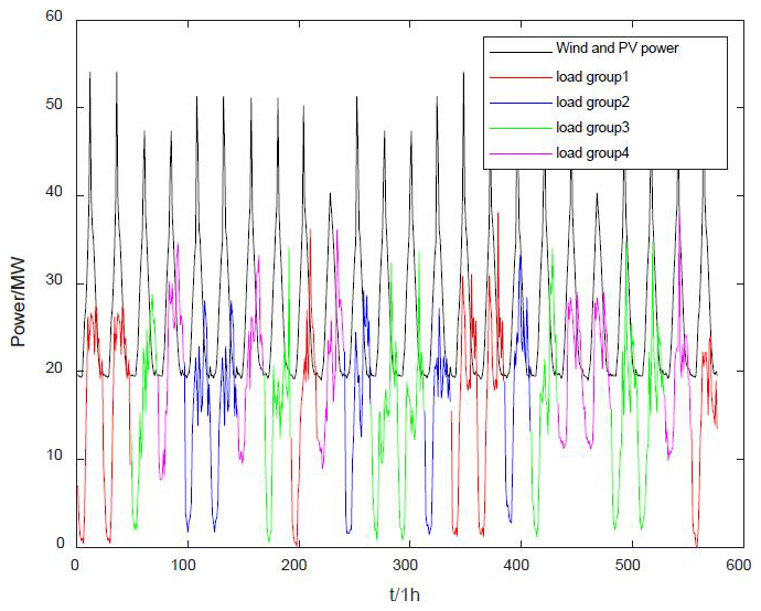
According to the method described in this paper, the matching results are shown in Fig. 4, and the wind–solar output is based on the principle that the highest-matching degree will meet different loads daily. As shown in the figure, the load-tracking evaluation criteria established in this paper can select the load with the most closely matched output among different loads for matching, reducing the grid-side pressure on both sides of the independent dispatch. At the same time, the load side is split into different load groups. The wind–solar output has excess energy at a specific period, which is used to charge the energy storage so that the energy storage has a specific dispatch interval on the days when the load is not matched. The suppressing time of the energy storage can be further extended.

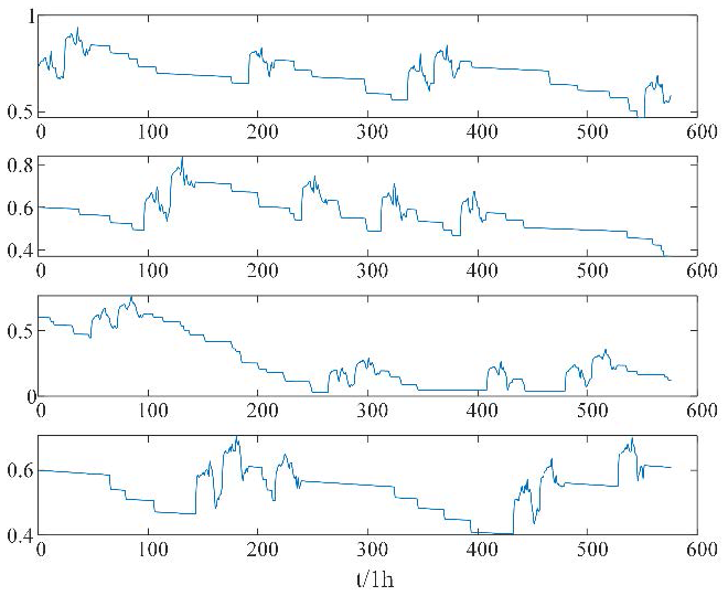
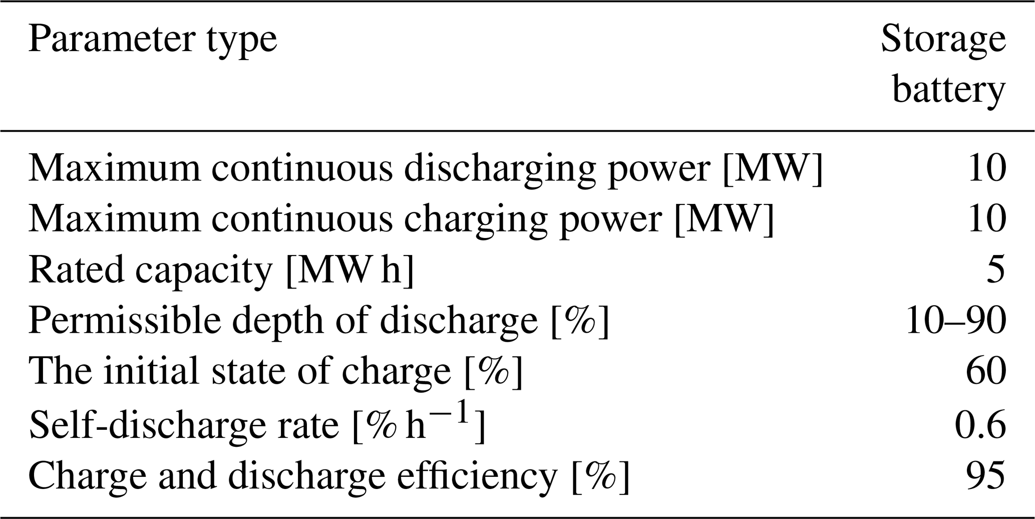
As shown in Fig. 5, the SOC of each load-side edge energy storage is optimized using the overall load fluctuation in the region and using the gray-wolf-optimization algorithm. The figure shows that source–load matching can provide enough energy for the energy storage to meet its required smoothing objective, and the SOC of each energy storage is maintained in the ideal interval to avoid damage to the energy storage lifetime. In this paper, the selected energy storage parameters are shown in Table 2.

Figure 5 Energy-storage SOC.

Table 2 Energy storage parameters.

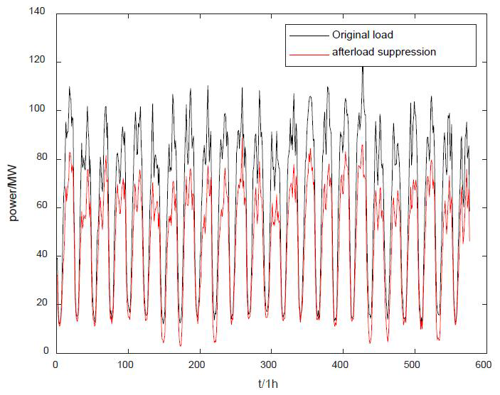
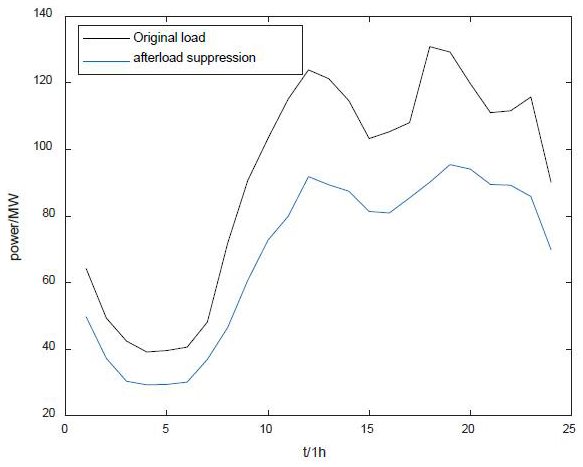
As shown in Fig. 6, the overall load power of the region is compared with the original regional load power after adopting the method proposed in this paper; the source–load matching strategy proposed in this paper can significantly reduce the power target of the grid-side load to be leveled and the pressure on the grid-side to meet the original load. At the same time, the method in this paper makes reasonable use of the regional wind–solar power and load adjacent to the characteristics of easy scheduling, the use of source–load matching strategy to achieve the power of local consumption, and the use of fluctuation suppression in the load to avoid possible waste of wind–solar power in a grid-connected energy waste situation that may exist.

Figure 6 Load-power changes before and after the suppression.

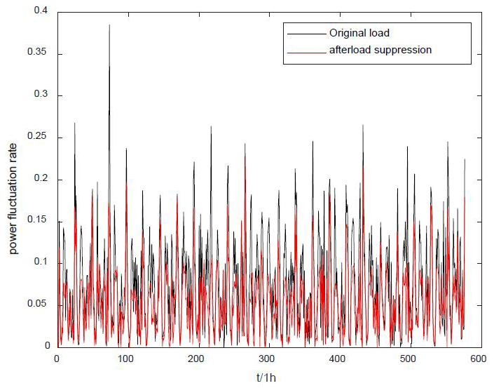
As shown in Fig. 7, the overall regional load fluctuation rate is compared with the original regional load fluctuation rate after adopting the proposed method in this paper. As shown in the figure, the proposed method can significantly reduce the fluctuation in the original regional load. The fluctuation of the original load can reach about 0.4, which is a tremendous pressure on the grid dispatch. However, after adopting the proposed method, the fluctuation rate of the regional load is reduced to less than 0.2, which reduces the difficulty of grid-side dispatch.

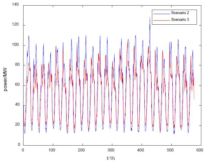
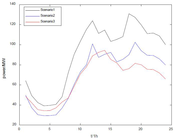
To further verify the effect of the proposed method on regional load fluctuation, three scenarios are set up in this paper for comparison: Scenario 1 is the traditional regional load suppression, i.e., the load power is completely satisfied by the grid side; Scenario 2 is the wind–solar system low-frequency output power used to satisfy the load power, while the energy storage suppresses a certain amount of excess wind–solar output and load fluctuation; and Scenario 3 is the proposed method.

In Fig. 8, the comparison between Scenario 2 and Scenario 3 is shown. As shown in the figure, compared with the direct use of wind–solar power to meet the load, the method proposed in this paper is more effective in suppressing the peak fluctuation of the load and reducing the load fluctuation rate. As Scenario 2 is the direct suppression of the low-frequency output of wind–solar power, the degree of load reduction in Scenario 2 is higher than that in Scenario 3 at the peak of wind–solar power output, which to some extent aggravates the pressure on the grid when the load rises at the next moment. The method proposed in this paper optimizes the charging and discharging of each energy storage unit to minimize the overall fluctuation of the regional load. It achieves this by reducing the load power during peak hours, charging the energy storage appropriately during load valleys and avoiding the fluctuation caused by over-satisfying the low valley load.

Figure 7 Changes in load volatility before and after smoothing.

Figure 8 Comparison of Scenario 2 and Scenario 3.

A comparison of the overall load power in the region for three scenarios on a randomly selected day is shown in Fig. 9. As shown in the figure, Scenario 3's overall fluctuation rate is smaller than Scenario 2's rate. The method proposed in this paper can provide overall smoothing of the split load while the remaining energy from the source–load matching is stored in the energy storage so that the load can be smoothed to some extent even when it is not matched. Compared with Scenario 2, Scenario 3 has a higher load power part of the time, which is because the objective of the proposed method is to reduce the overall volatility of the load, so part of the wind–solar power is used to charge the energy storage in that time. Compared with the traditional wind–solar power directly used to meet the load, the method proposed in this paper can divide the load reduction of a single period into the reduction of multiple periods and realize the lowest fluctuation of the regional load as a whole.

Figure 9 Power comparison of different scenarios in a day.

Figure 10 Load prediction results based on LSTM.

In order to verify the effectiveness of this paper's method for intraday scheduling, this paper forecasts the load with a time scale of 1 h. It uses this paper's method for smoothing verification.

Figure 11 Predictive flattening results of the regional power grid on a certain day.

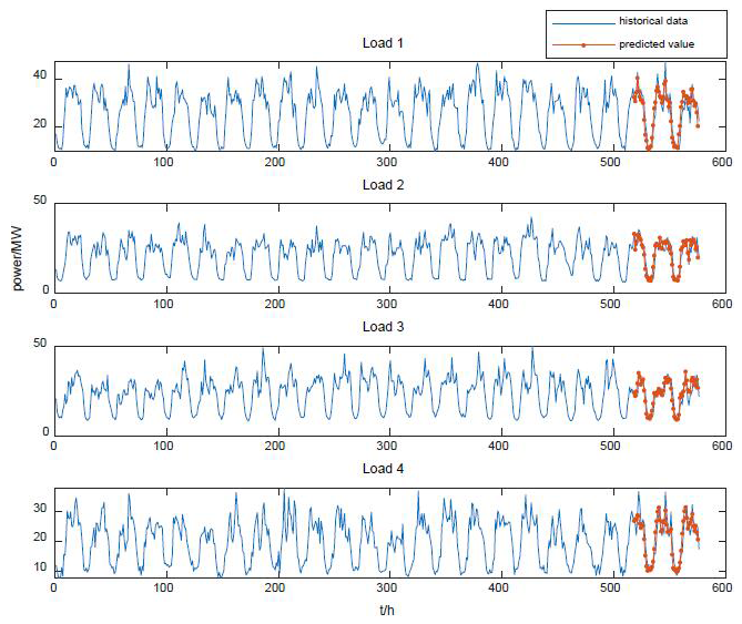
As shown in Fig. 10, the results of using long short-term memory (LSTM) to forecast each load based on historical data show that LSTM can forecast the load effectively. In operation scheduling, the next day's load can be predicted based on historical data. At the same time, the source-side output scenario is selected based on the weather, and the source–load matching strategy proposed in this paper is used to match the suppression. In the following sections, the forecast result of a particular day is selected to analyze the leveling.

As shown in Fig. 11, after forecasting the load on a particular day, the wind–solar power is selected to carry out source–load matching suppression, the results of the grid-connected load power in the region are compared to the wind–solar power and the marginal energy storage is suppressed for each load. After using the method in this paper, the overall grid-connected power of the regional load is significantly reduced. At the same time, the peak-load fluctuations are significantly reduced – such as, between 12:00–14:00 and 16:00–20:00 LT – where the original grid-connected load shows significant peaks. These peaks place considerable pressure on grid scheduling. After the suppression of the fluctuation strategy is applied, the resulting smoother load profile reduces the negative impact on grid-connected exchanges.

Figure 12 shows the change in the SOC of each edge energy-storage unit after the leveling-off point on the forecast day. As shown in the figure, the wind–solar power output on that day is matched with the fourth load group. After the wind–solar power output meets the load demand, the excess energy is used to charge the corresponding energy storage units, so the edge energy storage of the matched load can be kept in a good state for the duration of the day. At the same time, it can be seen from the change in the SOC of other marginal energy storage units that on an unmatched day, the marginal energy storage corresponding to each load group is appropriately discharged during peak load fluctuations to help reduce overall load fluctuation. At the same time, to make sure that the load group matches with wind–solar power for many consecutive days, the energy storage does not release all of the stored energy at one time so that the leveling-off time of the storage is prolonged as much as possible. The utilization of the storage is improved. To extend the leveling time and improve the utilization of energy storage as much as possible, the energy storage will not release all of its stored energy at once.

Figure 12 Day SOC status of edge energy storage.

Figure 13 Comparison forecast of daily volatility before and after flattening.

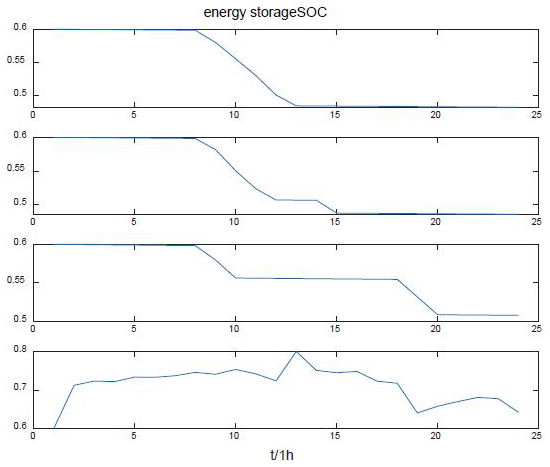
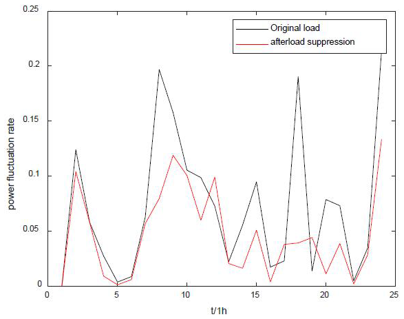
Figure 13 compares grid-connected volatility before and after load suppressing of the regional grid on the forecast day; as demonstrated in the figure, the volatility of the grid-connected load after using the method of this paper is significantly reduced, avoiding peak values of fluctuations. The grid-connected volatility of the original load has reached 0.2 many times. In contrast, the volatility after suppressing is maintained at 0.1 or below, which verifies the effectiveness of the method of this paper for the suppression of grid-connected load.

5 Conclusion

This paper addresses the shortcomings of wind–solar power output for load suppressing in the region. We also consider the smoother wind–solar power low-frequency output and source–load matching strategy for regional load smoothing. The proposed method has several significant features and contributions:

1. Framework development. A regional grid framework of “one source with multiple loads” is proposed. This framework effectively utilizes the low-frequency output of wind–solar power, which is more stable, to match and smooth the load fluctuations. By dividing the load into multiple groups and matching them with the source-side output, the method reduces the overall load fluctuation and the pressure on the grid-side dispatch.

2. Optimization algorithm. The gray-wolf-optimization algorithm based on Tent chaotic mapping is introduced. This algorithm enhances the global and local optimization capabilities, ensuring that the edge energy storage at each load side is optimized to minimize the overall load fluctuation. The algorithm's chaotic mapping feature helps to avoid local optima and achieves a more robust solution.

3. Local consumption and grid pressure reduction. The method effectively promotes the local consumption of wind–solar power and reduces the pressure on grid-side dispatch. By matching the source and load, the method ensures that renewable energy is utilized more efficiently, reducing the need for grid support and improving the overall stability of the regional power system.

4. High-complementarity utilization. The method fully utilizes the high complementarity of wind and solar power in the low-frequency band. This complementarity helps in reducing the uncertainty and volatility of renewable energy sources, making the power output more predictable and manageable.

5. Volatility reduction. The method significantly reduces the volatility of the regional power grid. By optimizing the charging and discharging strategies of edge energy storage, the method ensures that the load fluctuations are minimized, reducing the difficulty of grid-side dispatch and improving the reliability of the power system.

In summary, the proposed method provides a comprehensive solution to the challenges of integrating renewable energy into the grid. It not only improves the efficiency of renewable energy utilization but also enhances the stability and reliability of the power system. The method's ability to match the source and load effectively and optimize energy storage operations makes it a valuable tool for regional grid management. Future work will focus on further refining the model and exploring its application in different regional and operational contexts to maximize its potential in promoting sustainable energy use and grid stability.