Offshore wind farm layout optimization with alignment constraints

Wind farm layout optimization involves placing wind turbines in a defined domain to minimize the expected production losses due to wake effects within the wind farm. Due to navigational regulations and risks, tenders for offshore wind farms often impose so-called alignment constraints; i.e., wind turbines must be located at the intersections of a grid formed by parallelograms. The shape and orientation of these parallelograms are to be determined to minimize wake losses. Mathematically, this problem belongs to the class of non-convex, nonlinear mixed-integer programming problems, known to be highly complex. The literature has not yet investigated the wind farm layout optimization problem under alignment constraints. This paper makes two contributions. First, we propose a modelization of the annual energy production (AEP) maximization with alignment constraints as a mixed-integer nonlinear problem, where the continuous parameters are the parallelogram-based tiling parameters and the discrete variables are the turbines' positions at the tiling's intersections. Second, we provide a heuristic derived from the DEBO algorithm developed by the same team and presented in Thomas et al. (2023). The proposed method is the subject of international patent application number WO 2024/061627.

1 Introduction

Selecting the proper layout is a crucial task when building a wind farm. A layout far from optimal is prone to significant loss of expected annual energy production (AEP) due to wake effects within the farm. Having an optimized method of turbine placement in a given area helps maximize energy production over the wind farm's lifespan. In its full generality, the problem of optimizing a wind farm layout is a complex one for several reasons. The first is that computing a given farm's mean annual energy production is numerically complex; i.e., evaluating the optimization problem's objective function is computationally time-consuming (LoCascio et al., 2024; Porté-Agel et al., 2020). The second difficulty is that the problem is not convex; i.e., neither the objective function nor the minimization set are convex. As a result, the problem of wind farm layout optimization necessitates the development of dedicated optimization tools. Wind farm optimization has been the subject of much scientific research; see, for example, Herbert-Acero et al. (2014), Fischetti and Pisinger (2019), and Hou et al. (2019) for a list of reviews of such methods. Let us now focus on recent contributions to the field. In Quick et al. (2023), the authors develop a stochastic gradient-based method for optimizing wind farm layouts. The presented algorithm is developed for circular or square domains and could be easily extended to convex domains but not to non-convex or non-connected ones. In Kumar and Sharma (2023), the authors use a teaching–learning-based algorithm to solve the wind farm layout optimization problem for a circular domain. In Liang and Liu (2023), the authors use genetics and particle swarm algorithms to solve the problem on a square domain. In Fischetti and Fischetti (2022), the authors propose a mixed-integer linear programming model to solve turbine placement and cable routing optimization problems. In Kunakote et al. (2022), the authors compare 12 meta-heuristic methods for wind farm layout optimization. The presented methods do not rely on any assumption on the shape of the admissible domain. However, the method relies on a very coarse discretization of the domain and can be numerically intractable using a finer one. In Thomas et al. (2023), the authors compare eight wind farm optimization methods and provide a benchmark case study for comparing algorithm performances. The proposed benchmark is highly complex since the admissible domain is neither convex nor connected. However, this contribution does not account for any alignment constraints. Finally, in Stanley and Ning (2019), the authors propose a so-called inner-grid wind farm layout parameterization that satisfies strong alignment constraints. However, the authors assume a one-to-one correspondence between this parameterization and the layout configuration, which dramatically reduces the degree of freedom and potentially leads to far-from-optimal solutions. In fact, despite the extensive literature on wind farm optimization, to the best of our knowledge, no other method can handle turbine alignment constraints. By alignment constraint, we mean that we place the turbines at the intersections of a regular grid composed of parallelograms, whose shape and orientation are to be determined, while considering the possibility of not occupying all the grid's intersections. This possibility is a key feature of the proposed algorithm, and its interest is illustrated in the numerical examples presented in the paper. Far from being just an academic question, turbine alignment constraints are often imposed by maritime authorities on developers in practice to ensure the safe navigation of boats within the wind farm (see, for example, the following technical reports: Ministry of Transport of the French Republic, 2017, and Maritime and Coastguard Agency, 2012). The contribution of this paper is to provide an optimization algorithm for wind farm layout optimization that can handle alignment constraints. Mathematically, these alignment constraints render the wind farm layout optimization problem a mixed-integer nonlinear programming (MINLP) problem. The integer variables represent the positions of the turbines, which are restricted to the finite set of grid intersections within the admissible domain. The continuous variables are the grid parameters, that is to say the size and orientation of the grid's unit parallelogram. The nonlinearity mainly stems from the wind farm's annual energy production (AEP) as a function of the optimization parameters. These problems are generally extremely difficult to solve. As detailed in Burer and Letchford (2012), solving algorithms for non-convex MINLPs fall into two different categories: exact methods and heuristic-based methods. Exact methods often rely on branch-and-bound methods (Papadimitriou and Steiglitz, 1998) or separation properties of the objective function. Heuristic methods include tabu research (Exler et al., 2008), particle swarm algorithms (Yiqing et al., 2007; Young et al., 2007), genetic algorithms (Schlüter et al., 2009), or local-search methods (Liberti et al., 2011). The strategy adopted in this paper is to adapt the DEBO method developed by the authors in Thomas et al. (2023) to the problem at hand. This method is a local-search-based approach coupled with an exploration heuristic for optimizing parameters. The paper is organized as follows. In Sect. 2, we introduce useful notations and definitions. In Sect. 3, we describe the aligned-layout optimization problem; that is to say, we present the objective function, the constraints, and the optimization variables. We fully describe the optimization algorithm in Sect. 4. In Sect. 5, we take up the benchmark presented in Thomas et al. (2023) and add the alignment constraints, and we conduct a thorough study on the setting of the optimization algorithm hyper-parameters. In Sect. 6, we illustrate the impact of the alignment-grid parameters exploration method on the AEP and prove that an efficient exploration method yields a strong improvement in the AEP. Finally, in Sect. 7, we give the conclusions of this work and draw up research perspectives on the subject.

2 Notations and definitions

Throughout the paper we will use recurrently the following notations:

• $\mathbb{R},{\mathbb{R}}_{+}$ denote respectively the set of real numbers and the set of non negative real numbers.

• $\mathbb{Z},{\mathbb{Z}}_{*}$ denote respectively the set of integers and the set of non-zero integers.

• Ω∈ℝ² denotes two-dimensional domain where turbines can be planted.

• N_max denotes maximal number of turbines to be placed within the admissible domain E.

• D_turb denotes turbine diameter.

• D_min denotes minimal distance between turbines.

• D_max denotes maximal distance between turbines.

• w_s denotes wind speed.

• w_d denotes wind direction.

• ⊤ denotes logical true.

• ⊥ denotes logical false.

• ¬ denotes logical negation.

• ∧ denotes logical and operator.

• ∨ denotes logical or operator.

Definition 1. (Wind farm). A capital bold character associated with a subscript such as F_n denotes a n-turbine wind farm. Mathematically F_n is a function satisfying

$$\begin{array}{}\text{(1)}& {\mathbf{F}}_n:\mathit{\{}\mathrm{1},\mathrm{\dots },n\mathit{\}}\ni k\mapsto (x_k{y}_k{)}^{\top }\in {\mathbb{R}}^{\mathrm{2}},\end{array}$$

where (x_k  y_k)^⊤ is the position of the kth turbine. Let F_n and let $(xy{)}^{\top }\in {\mathbb{R}}^{\mathrm{2}}$; we denote ${\mathbf{H}}_{n+\mathrm{1}}:={\mathbf{F}}_n\oplus \left(xy\right)$ the wind farm defined as follows.

$$\begin{array}{}\text{(2)}& {\mathbf{H}}_{n+\mathrm{1}}\left(k\right):=\left\{\begin{array}{ll}{\mathbf{F}}_n\left(k\right)& \text{if}k\le n\\ (xy{)}^{\top }& \text{if}k=n+\mathrm{1}\end{array}\right.\end{array}$$

Definition 2. (Wind farm power production). We denote $\mathcal{P}:({\mathbf{F}}_n,w_{\mathrm{s}},w_{\mathrm{d}})\mapsto {\mathbb{R}}_{+}$ the power production of the wind farm F_n for a wind speed w_s and a wind direction w_d.

Definition 3. (Expected power production and annual energy production). We denote $\mathrm{W}:=(w_{\mathrm{s}},w_{\mathrm{d}})\in {\mathbb{R}}_{+}\times [\mathrm{0},\mathrm{2}\mathit{\pi })$ the wind random variable, and we denote ℙ_W the probability measure on ${\mathbb{R}}_{+}\times [\mathrm{0},\mathrm{2}\mathit{\pi })$ associated with the random variable W. Finally, we denote 𝔼_W the expectation with respect to the probability ℙ_W, and the expected power production of a wind farm F_n is

$$\begin{array}{}\text{(3)}& {\mathbb{E}}_{\mathrm{W}}\left(\mathcal{P}\right({\mathbf{F}}_n,w_{\mathrm{s}},w_{\mathrm{d}}\left)\right):=\underset{{\mathbb{R}}_{+}\times [\mathrm{0},\mathrm{2}\mathit{\pi })}{\int }\mathcal{P}({\mathbf{F}}_n,w_{\mathrm{s}},w_{\mathrm{d}})\mathrm{d}{\mathbb{P}}_{\mathrm{W}}(w_{\mathrm{s}},w_{\mathrm{d}}),\end{array}$$

and the annual energy production of a wind farm F_n denoted AEP(F_n) is

$$\begin{array}{}\text{(4)}& \mathrm{AEP}\left({\mathbf{F}}_n\right):=\mathrm{8760}.{\mathbb{E}}_{\mathrm{W}}\left(\mathcal{P}\right({\mathbf{F}}_n,w_{\mathrm{s}},w_{\mathrm{d}}\left)\right).\end{array}$$

Finally, when the probability is discrete, i.e., ${\mathbb{P}}_{\mathrm{W}}:={\sum }_{n=\mathrm{1}}^{N_{\mathrm{W}}}p(w_{\mathrm{s}}^n,w_{\mathrm{d}}^n)\mathit{\delta }(w_{\mathrm{s}}^n,w_{\mathrm{d}}^n)$, where $p(w_{\mathrm{s}}^n,w_{\mathrm{d}}^n)$ is the probability of wind $W=(w_{\mathrm{s}}^n,w_{\mathrm{d}}^n)$ and $\mathit{\delta }(w_{\mathrm{s}}^n,w_{\mathrm{d}}^n)$ is the Dirac delta function at $(w_{\mathrm{s}}^n,w_{\mathrm{d}}^n)$, the AEP computation is

$$\begin{array}{}\text{(5)}& \mathrm{AEP}\left({\mathbf{F}}_n\right):=\mathrm{8760}\sum _{n=\mathrm{1}}^{N_{\mathrm{W}}}p(w_{\mathrm{s}}^n,w_{\mathrm{d}}^n)\mathcal{P}({\mathbf{F}}_n,w_{\mathrm{s}}^n,w_{\mathrm{d}}^n).\end{array}$$

3 Optimization model for layout optimization with alignment constraints

The optimization problem we are interested in consists of optimizing the grid configuration and the turbine placement on the intersections of this grid. This optimization problem is a nonlinear mixed-integer programming problem, a class of problems known to be challenging to solve. In this section, we describe the parameterization of our problem.

3.1 Grid parameterization

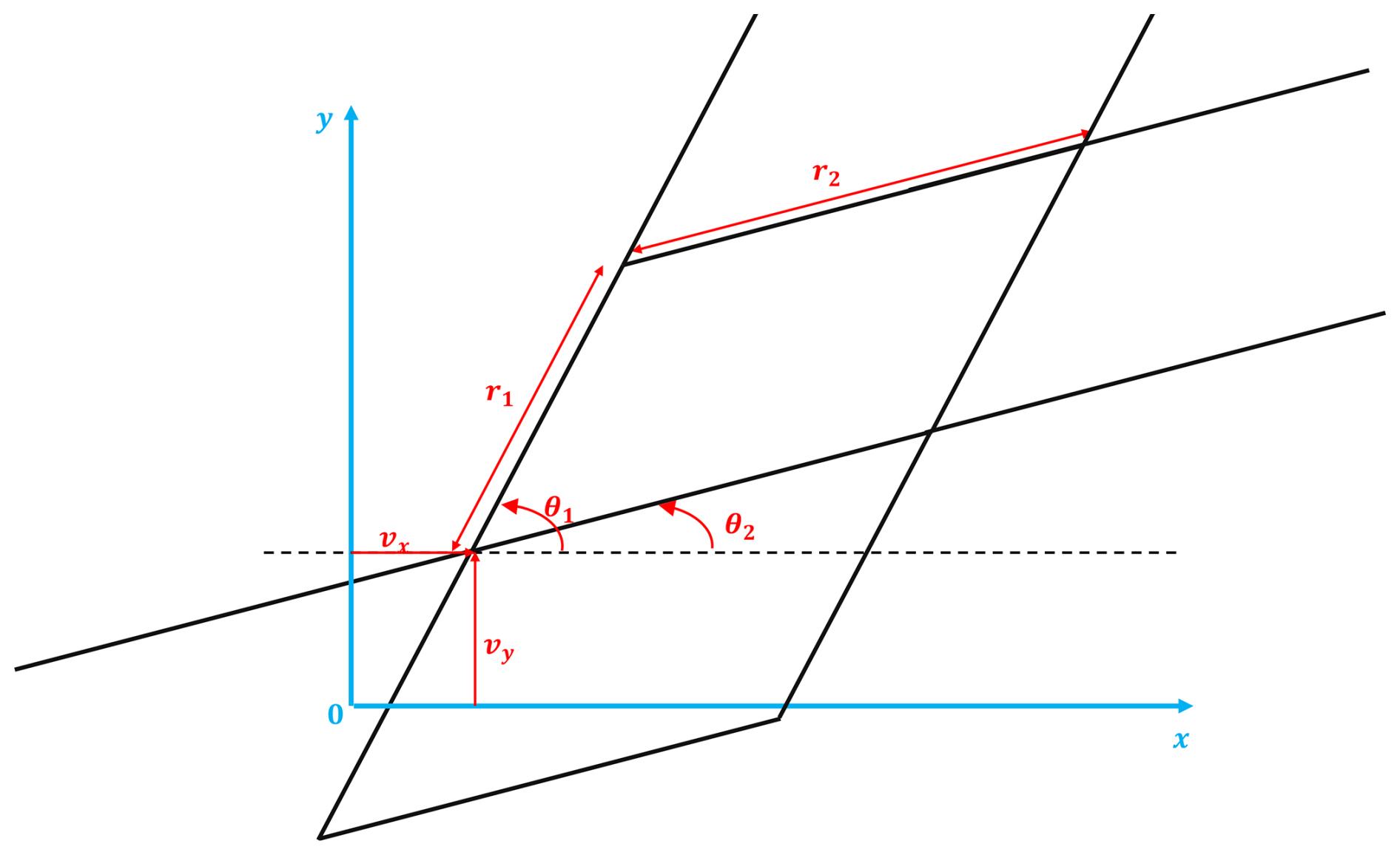
To write the optimization problem, we parameterize the grid using 6 parameters $(r_{\mathrm{1}},r_{\mathrm{2}},{\mathit{\theta }}_{\mathrm{1}},{\mathit{\theta }}_{\mathrm{2}},v_x,v_y)$ as represented in Fig. 1. The grid is a parallelogram-based tiling of the plane, the parameters r₁,r₂ are the two sides' length of the parallelogram, the parameter θ₁ (θ₂) is the angle formed between the side of the parallelogram of length r₁ (r₂) and the x axis. Finally the parameters v_x,v_y are the offset between the origin of the Cartesian and the parallelogram-based grids. Using this parameterization we define the change-of-basis matrix from the canonical basis denoted ℬ₀ to the grid basis denoted $\mathcal{B}({\mathit{\theta }}_{\mathrm{1}},{\mathit{\theta }}_{\mathrm{2}},r_{\mathrm{1}},r_{\mathrm{2}})$ as follows.

$$\begin{array}{}\text{(6)}& P_{{\mathcal{B}}_{\mathrm{0}}}^{\mathcal{B}({\mathit{\theta }}_{\mathrm{1}},{\mathit{\theta }}_{\mathrm{2}},r_{\mathrm{1}},r_{\mathrm{2}})}=\left(\begin{array}{ll}{r}_{\mathrm{1}}\cos \left({\mathit{\theta }}_{\mathrm{1}}\right)& r_{\mathrm{2}}\cos \left({\mathit{\theta }}_{\mathrm{2}}\right)\\ r_{\mathrm{1}}\sin \left({\mathit{\theta }}_{\mathrm{1}}\right)& r_{\mathrm{2}}\sin \left({\mathit{\theta }}_{\mathrm{2}}\right)\end{array}\right)\end{array}$$

In the grid-basis coordinates, any intersection point p is as follows.

$$p:=\left(\begin{array}{c}{k}_{\mathrm{1}}\\ k_{\mathrm{2}}\end{array}\right)+{\left(P_{{\mathcal{B}}_{\mathrm{0}}}^{\mathcal{B}({\mathit{\theta }}_{\mathrm{1}},{\mathit{\theta }}_{\mathrm{2}},r_{\mathrm{1}},r_{\mathrm{2}})}\right)}^{-\mathrm{1}}\left(\begin{array}{c}{v}_x\\ v_y\end{array}\right)k_{\mathrm{1}},k_{\mathrm{2}}\in \mathbb{Z}$$

This parameterization in grid basis is, in turn, equivalent to

$$\begin{array}{}\text{(7)}& p=\left(\begin{array}{l}{k}_{\mathrm{1}}\\ k_{\mathrm{2}}\end{array}\right)+\left(\begin{array}{l}{\mathrm{\Delta }}_{\mathrm{1}}\\ {\mathrm{\Delta }}_{\mathrm{2}}\end{array}\right)k_{\mathrm{1}},k_{\mathrm{2}}\in \mathbb{Z}\text{and}{\mathrm{\Delta }}_{\mathrm{1}},{\mathrm{\Delta }}_{\mathrm{2}}\in [\mathrm{0},\mathrm{1}).\end{array}$$

Figure 1 Grid parameterization for aligned layout.

3.2 Layout parameterization

Using the grid parameterization described in Sect. 3.1, an aligned layout has its turbines located on the intersections of the grid which is

$$\begin{array}{}\text{(8)}& \begin{array}{rl}& \mathbf{F}\left[\mathcal{B}{]}_n\right(i):\mathit{\{}\mathrm{1},\mathrm{\dots },n\mathit{\}}\ni i\mapsto {\left(\begin{array}{cc}{k}_{\mathrm{1}}^i& k_{\mathrm{2}}^i\end{array}\right)}^{\top }+{\left(\begin{array}{cc}{\mathrm{\Delta }}_{\mathrm{1}}& {\mathrm{\Delta }}_{\mathrm{2}}\end{array}\right)}^{\top },\\ & k_{\mathrm{1}}^i,k_{\mathrm{2}}^i\in \mathbb{Z};{\mathrm{\Delta }}_{\mathrm{1}},{\mathrm{\Delta }}_{\mathrm{2}}\in [\mathrm{0},\mathrm{1}).\end{array}\end{array}$$

The corresponding wind farm in canonical coordinates F_n thus is

$$\begin{array}{}\text{(9)}& {\mathbf{F}}_n\left(i\right)=P_{{\mathcal{B}}_{\mathrm{0}}}^{\mathcal{B}({\mathit{\theta }}_{\mathrm{1}},{\mathit{\theta }}_{\mathrm{2}},r_{\mathrm{1}},r_{\mathrm{2}})}\mathbf{F}\left[\mathcal{B}{]}_n\right(i),i=\mathrm{1},\mathrm{\dots },n.\end{array}$$

Thanks to the parameterization from Eq. (8), the alignment constraint translates into an integer constraint on the optimization variables $(k_{\mathrm{1}}^i,k_{\mathrm{2}}^i)$.

3.3 Optimization problem

We are now ready to write the general wind farm layout optimization problem with alignment constraints. This optimization problem consists of maximizing the wind farm's annual energy production as defined in Eq. (4). This is

$$\begin{array}{}\text{(10)}& \underset{(k_{\mathrm{1}}^i,k_{\mathrm{2}}^i{)}_{i=\mathrm{1},\mathrm{\dots },N_{max}},{\mathrm{\Delta }}_{\mathrm{1}},{\mathrm{\Delta }}_{\mathrm{2}},r_{\mathrm{1}},r_{\mathrm{2}},{\mathit{\theta }}_{\mathrm{1}},{\mathit{\theta }}_{\mathrm{2}}}{max}\mathrm{AEP}\left(\mathbf{F}\right[\mathcal{B}{]}_{N_{max}})\end{array}$$

under the following constraints.

$$\begin{array}{}\text{(11)}& {\displaystyle }{k}_{\mathrm{1}}^i,k_{\mathrm{2}}^i\in \mathbb{Z};i=\mathrm{1},\mathrm{\dots },N_{max}\text{(12)}& {\displaystyle }\left|k_{\mathrm{1}}^i-k_{\mathrm{1}}^j\right|+\left|k_{\mathrm{2}}^i-k_{\mathrm{2}}^j\right|\ge \mathrm{1};\forall i\ne j\text{(13)}& {\displaystyle }{\mathrm{\Delta }}_{\mathrm{1}},{\mathrm{\Delta }}_{\mathrm{2}}\in [\mathrm{0},\mathrm{1})\text{(14)}& {\displaystyle }{\mathbf{F}}_{N_{max}}\left(i\right)\in \mathrm{\Omega };i=\mathrm{1},\mathrm{\dots },N_{max}\text{(15)}& {\displaystyle }{\mathit{\theta }}_{\mathrm{1}}\in \left(-{\displaystyle \frac{\mathit{\pi }}{\mathrm{2}}},{\displaystyle \frac{\mathit{\pi }}{\mathrm{2}}}\right]\text{(16)}& {\displaystyle }{\mathit{\theta }}_{\mathrm{2}}\in \left[-{\displaystyle \frac{\mathit{\pi }}{\mathrm{2}}},{\mathit{\theta }}_{\mathrm{1}}\right)\text{(17)}& {\displaystyle }{D}_{min}\le \underset{\mathit{z}\in {\mathbb{Z}}_{*}^{\mathrm{2}}}{min}∥P_{{\mathcal{B}}_{\mathrm{0}}}^{\mathcal{B}({\mathit{\theta }}_{\mathrm{1}},{\mathit{\theta }}_{\mathrm{2}},r_{\mathrm{1}},r_{\mathrm{2}})}z∥\end{array}$$

Equations (11), (12), and (13) ensure that the turbines are located at the intersections of the grid defined by the parameters $(r_{\mathrm{1}},r_{\mathrm{2}},{\mathit{\theta }}_{\mathrm{1}},{\mathit{\theta }}_{\mathrm{2}},v_x,v_y)$ and thus that the turbines are aligned along the directions θ₁ and θ₂. The constraint from Eq. (14) guarantees that the turbines are located in the admissible domain. Constraints defined in Eqs. (15) and (16) allow us to generate all possible parallelogram-based grids. We only consider ${\mathit{\theta }}_{\mathrm{1}}\in (-\mathit{\pi }/\mathrm{2},\mathit{\pi }/\mathrm{2}]$ since ${\mathit{\theta }}_{\mathrm{1}}>\mathit{\pi }/\mathrm{2}$ (${\mathit{\theta }}_{\mathrm{1}}<-\mathit{\pi }/\mathrm{2}$) yields the same tiling as ${\mathit{\theta }}_{\mathrm{1}}-\mathit{\pi }/\mathrm{2}$ (${\mathit{\theta }}_{\mathrm{1}}+\mathit{\pi }/\mathrm{2}$). Finally, the constraint from Eq. (17) ensures that no grid's intersections are closer to each other than D_min. Since the turbines are necessarily located on these intersections, this constraint ensures that turbines are at least D_min distant from each other.

4 Solving algorithm

4.1 General description of the proposed solving algorithm

The method presented in this paper belongs to the category of heuristic-based methods and consists of the following steps.

• STEP 1. The first step consists of computing the set R_1,2 of parameters (r₁,r₂) by discretization of the space ${\left[D_{min},D_{max}\right]}^{\mathrm{2}}$ using a grid size of Δr. There is no upper limit to the D_max value. However, it is useless to set this parameter at a large value. Indeed, beyond a certain value $d>D_{min}$, any shape-parameter configuration such that $r_{\mathrm{1}},r_{\mathrm{2}}>d$ will produce coarse grids with fewer than N_max admissible intersections.

• STEP 2. The second step consists of reducing the size of the angle search space. To do so, for each couple $(r_{\mathrm{1}},r_{\mathrm{2}})\in R_{\mathrm{1},\mathrm{2}}$, we discretize the search space $\left(-\frac{\mathit{\pi }}{\mathrm{2}},\frac{\mathit{\pi }}{\mathrm{2}}\right]\times \left[-\frac{\mathit{\pi }}{\mathrm{2}},{\mathit{\theta }}_{\mathrm{1}}\right)$ using a discretization size of Δθ. Then, for each grid configuration $(r_{\mathrm{1}},r_{\mathrm{2}},{\mathit{\theta }}_{\mathrm{1}}^k,{\mathit{\theta }}_{\mathrm{2}}^k{)}_k$ satisfying Eq. (17) we compute the AEP of an elementary 4-turbine wind farm. Then, we store the N_θ best angle configurations (θ₁,θ₂) in an angle set Θ. This latter set Θ is the reduced angle search space.

• STEP 3. Then, we compute a set of grid configurations $(r_{\mathrm{1}},r_{\mathrm{2}},{\mathit{\theta }}_{\mathrm{1}},{\mathit{\theta }}_{\mathrm{2}})$ defined as $\mathrm{grids}:=\mathit{\left\{}\right(r_{\mathrm{1}},r_{\mathrm{2}},{\mathit{\theta }}_{\mathrm{1}},{\mathit{\theta }}_{\mathrm{2}}):(r_{\mathrm{1}},r_{\mathrm{2}})\in R_{\mathrm{1},\mathrm{2}},({\mathit{\theta }}_{\mathrm{1}},{\mathit{\theta }}_{\mathrm{2}})\in \mathrm{\Theta },\mathrm{Eq}$. (17) holds}.

• STEP 4. For each explored shape configuration $(r_{\mathrm{1}},r_{\mathrm{2}},{\mathit{\theta }}_{\mathrm{1}},{\mathit{\theta }}_{\mathrm{2}})$, we compute an optimal layout using a greedy algorithm for placing the N_max turbines on the intersections of the grid and using a local-search optimization method to move the turbines on the intersections. The sequence of greedy initialization followed by a local-search method has already been proved efficient for wind farm layout optimization without alignment constraints; see the DEBO algorithm from Thomas et al. (2023).

• STEP 5. Return the best overall wind farm layout.

Finally, the corresponding pseudo-code is displayed in Algorithm 1. As one can see on line 13, step 4, which is the most computationally demanding, can be run in parallel.

Algorithm 1 Aligned_Optimization$(\mathrm{\Omega },N_{max},N_{\mathit{\theta }},D_{min}$, $D_{max},\mathrm{\Delta }r,\mathrm{\Delta }\mathit{\theta })$.

1:

{STEP 1 : Compute R_1,2}

2:

$R_{\mathrm{1},\mathrm{2}}\leftarrow$ GenerateR1R2$(\mathrm{\Delta }r,D_{min},D_{max})$

3:

4:

{STEP 2 : Compute Reduced Angles Search Space Θ}

5:

Θ← ReduceSearchSpace$(R_{\mathrm{1},\mathrm{2}},\mathrm{\Delta }\mathit{\theta },D_{min},D_{max},D_{\mathrm{turb}},N_{\mathit{\theta }})$

6:

7:

{STEP 3 : Generate compute admissible intersections for each grid configurations}

8:

grids← GenerateConfigs$(R_{\mathrm{1},\mathrm{2}},\mathrm{\Theta },D_{min},D_{max},D_{\mathrm{turb}})$

9:

intersections_sets← ComputeAllIntersections($\mathrm{grids},D_{min},\mathrm{\Omega }$)

10:

11:

{STEP 4 : Compute optimal layout for each set of intersections}

12:

layouts←∅

13:

for $(\mathrm{intersections},(r_{\mathrm{1}},r_{\mathrm{2}},{\mathit{\theta }}_{\mathrm{1}},{\mathit{\theta }}_{\mathrm{2}}\left)\right)\in \mathrm{intersections}\mathit{\_}\mathrm{sets}$ {Run in parallel} do

14:

$\left({\mathbf{F}}_{N_{max}},\mathrm{aep}\right)\leftarrow$ PlaceTurbines(intersections)

15:

$\mathrm{layouts}\leftarrow \mathrm{layouts}\bigcup \mathit{\left\{}\right({\mathbf{F}}_{N_{max}},\mathrm{aep},\mathrm{intersections}$, $(r_{\mathrm{1}},r_{\mathrm{2}},{\mathit{\theta }}_{\mathrm{1}},{\mathit{\theta }}_{\mathrm{2}})\left)\mathit{\right\}}$

16:

end for

17:

layouts←sort(layouts) by aep in descending order

18:

19:

{STEP 5 : Get best overall layout}

20:

return  layouts(0)

4.2 Angle search space reduction and grid configuration selection

In this section, we describe the first part of the algorithm which consists of finding a set of grid configurations $(r_{\mathrm{1}},r_{\mathrm{2}},{\mathit{\theta }}_{\mathrm{1}},{\mathit{\theta }}_{\mathrm{2}})$ of reasonable size and performing a complete wind farm layout optimization for each element of this set. To do so, we first compute the set R_1,2 of parameters (r₁,r₂) by discretizing the space ${\left[D_{min},D_{max}\right]}^{\mathrm{2}}$ using a discretization of size Δr. Then, for each $(r_{\mathrm{1}},r_{\mathrm{2}})\in R_{\mathrm{1},\mathrm{2}}$, discretize the following search space

$$\begin{array}{}\text{(18)}& S:=\left\{({\mathit{\theta }}_{\mathrm{1}},{\mathit{\theta }}_{\mathrm{2}})\in {\left[-{\displaystyle \frac{\mathit{\pi }}{\mathrm{2}}},{\displaystyle \frac{\mathit{\pi }}{\mathrm{2}}}\right]}^{\mathrm{2}}:{\mathit{\theta }}_{\mathrm{1}}\ge -{\displaystyle \frac{\mathit{\pi }}{\mathrm{2}}}+\mathrm{\Delta }\mathit{\theta },{\mathit{\theta }}_{\mathrm{2}}\le {\mathit{\theta }}_{\mathrm{1}}-\mathrm{\Delta }\mathit{\theta }\right\}\end{array}$$

with an angle discretization parameter Δθ. We denote S_D this discrete search space. Then, for each $(r_{\mathrm{1}},r_{\mathrm{2}})\in R_{\mathrm{1},\mathrm{2}}$, we define the corresponding angle search space ${\mathrm{\Theta }}_{r_{\mathrm{1}},r_{\mathrm{2}}}$ as follows.

$$\begin{array}{}\text{(19)}& {\mathrm{\Theta }}_{r_{\mathrm{1}},r_{\mathrm{2}}}:=\left\{({\mathit{\theta }}_{\mathrm{1}},{\mathit{\theta }}_{\mathrm{2}})\in S_{\mathrm{D}}:\mathrm{Eq}.\left(\mathrm{17}\right)\mathrm{holds}\right\}\end{array}$$

Then, for each configuration $(r_{\mathrm{1}},r_{\mathrm{2}},{\mathit{\theta }}_{\mathrm{1}}^k,{\mathit{\theta }}_{\mathrm{2}}^k{)}_k$ with $({\mathit{\theta }}_{\mathrm{1}}^k,{\mathit{\theta }}_{\mathrm{2}}^k)\in {\mathrm{\Theta }}_{r_{\mathrm{1}},r_{\mathrm{2}}}$ we compute the AEP of the elementary farms
$\left(\mathbf{F}\right[\mathcal{B}(r_{\mathrm{1}},r_{\mathrm{2}},{\mathit{\theta }}_{\mathrm{1}}^k,{\mathit{\theta }}_{\mathrm{2}}^k){]}_{\mathrm{4}}{)}_k$ defined as follows,

$$\begin{array}{}\text{(20)}& \mathbf{F}\left[\mathcal{B}\right(r_{\mathrm{1}},r_{\mathrm{2}},{\mathit{\theta }}_{\mathrm{1}}^k,{\mathit{\theta }}_{\mathrm{2}}^k\left){]}_{\mathrm{4}}\right(i):=\left\{\begin{array}{ll}(\mathrm{0}\mathrm{0}{)}^{\top }& \mathrm{if}i=\mathrm{1},\\ (\mathrm{1}\mathrm{0}{)}^{\top }& \mathrm{if}i=\mathrm{2},\\ (\mathrm{0}\mathrm{1}{)}^{\top }& \mathrm{if}i=\mathrm{3},\\ (\mathrm{1}\mathrm{1}{)}^{\top }& \mathrm{if}i=\mathrm{4},\end{array}\right.\end{array}$$

and sort the couples $({\mathit{\theta }}_{\mathrm{1}}^k,{\mathit{\theta }}_{\mathrm{2}}^k{)}_i$ by decreasing order of AEP. Finally, for each $(r_{\mathrm{1}},r_{\mathrm{2}})\in R_{\mathrm{1},\mathrm{2}}$, we store in the set Θ the best N_θ angles configuration $({\mathit{\theta }}_{\mathrm{1}}^k,{\mathit{\theta }}_{\mathrm{2}}^k)\in {\mathrm{\Theta }}_{r_{\mathrm{1}},r_{\mathrm{2}}}$. Then, the continuous-variable search space denoted grids consists of all the combinations of the $(r_{\mathrm{1}},r_{\mathrm{2}})\in R_{\mathrm{1},\mathrm{2}}$ explored with all the angles' configuration from Θ, i.e.,

$$\begin{array}{}\text{(21)}& \begin{array}{rl}\mathrm{grids}& :=\mathit{\left\{}\right(r_{\mathrm{1}},r_{\mathrm{2}},{\mathit{\theta }}_{\mathrm{1}},{\mathit{\theta }}_{\mathrm{2}}):(r_{\mathrm{1}},r_{\mathrm{2}})\in R_{\mathrm{1},\mathrm{2}},({\mathit{\theta }}_{\mathrm{1}},{\mathit{\theta }}_{\mathrm{2}})\\ & \in \mathrm{\Theta }:\mathrm{Eq}.\left(\mathrm{17}\right)\mathrm{holds}\mathit{\}}.\end{array}\end{array}$$

The corresponding algorithm in pseudo-code is described in Algorithms A1, A2, A3, and A4.

4.3 Compute intersections for each grid configuration

This part of the algorithm consists of traversing grids(k) and, for each configuration $(r_{\mathrm{1}}^k,r_{\mathrm{2}}^k,{\mathit{\theta }}_{\mathrm{1}}^k,{\mathit{\theta }}_{\mathrm{2}}^k)$, calculating the maximum number of intersections located in the admissible domain Ω and their positions. If this set of intersections has more than N_max elements and if all intersections are D_min apart from each other, this set of intersections is stored in a set of intersections that we denote intersections_sets. The corresponding algorithm is written in pseudo-code in Algorithm A5.

4.4 Optimize turbines placement

4.4.1 Greedy initialization

Given a grid configuration $(r_{\mathrm{1}},r_{\mathrm{2}},{\mathit{\theta }}_{\mathrm{1}},{\mathit{\theta }}_{\mathrm{2}},{\mathrm{\Delta }}_{\mathrm{1}},{\mathrm{\Delta }}_{\mathrm{2}})$, a greedy algorithm is used to sequentially place N_max turbines on the admissible intersections. This algorithm consists of sequentially placing the turbines on the best possible empty intersection, in the sense of AEP maximization, until N_max turbines are placed. The corresponding algorithm in pseudo-code is given in Algorithm A6.

4.4.2 Local search

This part of the algorithm sequentially moves each turbine in random order from its current intersection to a free one if it provides a strict increase in AEP. The algorithm stops when a complete course of all the turbines has been made without a single one being moved. When the number of intersections in the admissible domain is much bigger than N_max, one can explore a subset of the free intersections. For example, one can explore the p closest intersections from the turbine to be moved or select p random free intersections. In this case, the size of the subset to explore and its definition, p, are user-defined parameters. The algorithm in pseudo-code is given in Algorithm A7.

4.4.3 Turbine placement optimization

Finally, given a set of intersections, the optimization algorithm for optimal turbine placement consists of using sequentially the greedy initialization and the local-search algorithm as described in pseudo-code in Algorithm A9.

5 Numerical examples

5.1 Problem presentation

For this numerical example, we use the same case study as in Thomas et al. (2023), whose data are available in Baker et al. (2021). The windrose corresponding to this case study is displayed in Fig. 2. This case study was created within the International Energy Association (IEA) Wind Task 37, and it is based on the Borssele III and IV wind farms. Of particular interest in this case study is the presence of five disconnected boundary regions and concave boundary features. The turbines are 10 MW machines with 198 m rotor diameters based on the IEA 10 MW reference wind turbine (Bortolotti et al., 2019). For the AEP computation, we also use the same algorithm as in Thomas et al. (2023). This method is based on a simple Gaussian wake model based on Bastankhah's Gaussian wake model (Bastankhah and Porté-Agel, 2016) and presented in the IEA case study 3 and 4 announcement documents (Baker et al., 2021) to calculate wind speeds at each turbine in the wind farm. However, any other AEP computation software, such as FLORIS (2023), can be used with the presented algorithm as long as the computation time of the AEP is fast enough. Indeed, our optimization algorithm requires a large number of AEP evaluations. Finally, the AEP is computed using a windrose discretized as follows.

$$\begin{array}{ll}{\displaystyle }& {\displaystyle }\mathrm{wind}\mathrm{direction}\mathrm{bins}=\mathit{\{}\mathrm{0},\mathrm{1},\mathrm{\dots },\mathrm{359}\mathit{\}}\\ {\displaystyle }& {\displaystyle }\mathrm{wind}\mathrm{speed}\mathrm{bins}=\mathit{\{}\mathrm{0.90},\mathrm{1.98},\mathrm{3.18},\mathrm{4.40},\mathrm{5.64},\mathrm{6.87},\mathrm{8.11},\\ {\displaystyle }& {\displaystyle }\mathrm{9.35},\mathrm{10.59},\mathrm{11.83},\mathrm{13.07},\mathrm{14.31},\mathrm{15.56},\mathrm{16.80},\mathrm{18.04},\\ {\displaystyle }& {\displaystyle }\mathrm{19.28},\mathrm{20.52},\mathrm{21.77},\mathrm{23.01},\mathrm{24.25}\mathit{\}}\end{array}$$

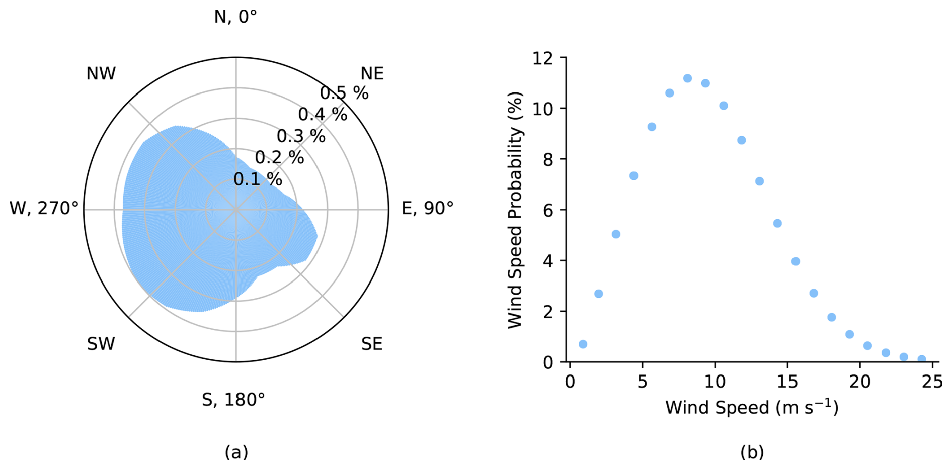
Figure 2 This figure, reproduced from Thomas et al. (2023), displays the full wind resource used for evaluating the final wind farm layouts. (a) The wind direction probability (360 bins). (b) A representative wind speed probability distribution (20 bins).

5.2 Influence of the hyper-parameters on the AEP and the computation time

The optimization procedure described in Sect. 4 requires setting 5 hyper-parameters: D_min, D_max, Δθ, N_θ, and Δr. The turbine's manufacturer usually sets D_min at a fixed value. In this example, we set $D_{min}=\mathrm{2}{D}_{\mathrm{turb}}$. The parameter D_max must be chosen large enough to allow a good exploration range for the grid parameters (r₁,r₂). However, setting D_max with a significant value generates grids with a number of admissible intersections smaller than the number of turbines to be placed, i.e., in generating non-admissible layouts. Therefore, we have set $D_{max}=\mathrm{6}{D}_{\mathrm{turb}}$. The parameter Δθ should be chosen to the minimal value such that the wake model used to compute the AEP is valid. For this example, we set Δθ=1°. The remaining hyper-parameters, N_θ and Δr, dramatically affect the optimization procedure regarding AEP value and computation time. Indeed, as explained in Sect. 4.2, the larger N_θ, the larger the reduced angle set denoted Θ, and the smaller Δr, the larger the set R_1,2. The number of configurations to optimize being the product of the cardinal of the sets Θ and R_1,2, the larger these sets, the longer the computation time. However, the more configuration to optimize, the greater the AEP. Therefore, any layout optimization needs to make a trade-off between computation time and size of the set of configuration to optimize. In this section, we will show the effect of the parameters N_θ and Δr on the optimal AEP and the computation time and give the user some guidelines to set these parameters. To do so, we run Algorithm 1 for all possible configurations of the hyper-parameters valued in their respective value set given in Table 1 for wind farm sizes of 81, 100, 150, and 250 turbines respectively. The numerical results of these optimizations are gathered in Table 2 and illustrated in Figs. 3 and 4. In Fig. 3, one can see that the expected power per turbine¹ is growing with respect to N_θ and decreasing with respect to Δr. Also, when N_θ≥5 and Δr≤1D_turb, the expected powers per turbine are similar whatever the value of these hyper-parameters. However, as illustrated in Fig. 4, the execution time is strongly increasing with respect to N_θ and strongly decreasing with respect to Δr. Therefore, if Algorithm 1 is run using an AEP computation method more precise and computationally more expensive than the one we used (see Baker et al., 2021; Thomas et al., 2023), keeping N_θ reasonably small (≈5) and Δr reasonably large (≈1) should enable the solving algorithm to find a well-performing layout in a reasonable execution time. In addition, as illustrated in Table 1, the solving algorithm often sets the optimal shape parameters (r₁,r₂) to their minimal authorized values. This behavior indicates that the method generates grids with many intersections and, thus, a large degree of freedom for the local-search part of the algorithm. The larger the degree of freedom for the local-search algorithm, the better the solution. The best layout for each wind farm size is displayed in Fig. 5, and the optimal parameters $(r_{\mathrm{1}},r_{\mathrm{2}},{\mathit{\theta }}_{\mathrm{1}},{\mathit{\theta }}_{\mathrm{2}})$, the optimal AEP, the optimal expected power per turbine, and the execution time are displayed in Table 3. The execution time corresponds to the total execution time. However, steps 1 to 3 from Algorithm 1 are always computed in less than 1.5 min (for Δr=0.5 and N_θ=10); the majority of the execution time is spent on step 4 of Algorithm 1.

Table 1 Value set of each hyper-parameter.

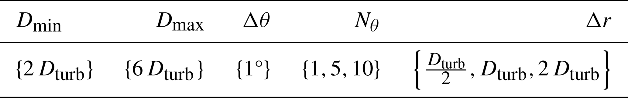
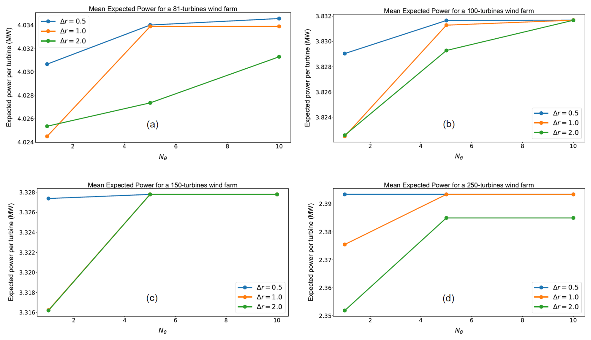
Figure 3 Expected power per turbine for 81-, 100-, 150-, and 250-turbine wind farms, displayed in panels (a), (b), (c), and (d) respectively, as a function of the hyper-parameters N_θ and Δr.

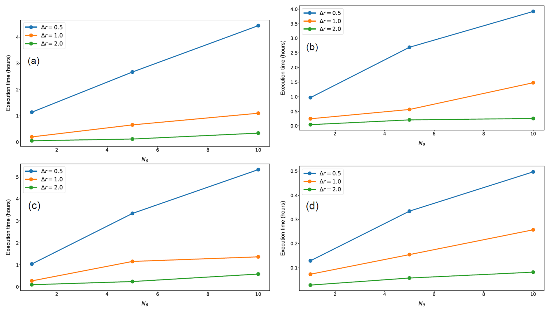
Figure 4 Execution time of Algorithm 1 for 81-, 100-, 150-, and 250-turbine wind farms, displayed in panels (a), (b), (c), and (d) respectively, as a function of the hyper-parameters N_θ and Δr. All optimizations were run on a 12th Gen Intel(R) i7-12700H 2.30 GHz core.

Table 2 Influence of the hyper-parameters N_θ and Δr on the AEP and Algorithm 1 execution time. All optimizations were run on a 12th Gen Intel(R) i7-12700H 2.30 GHz core.

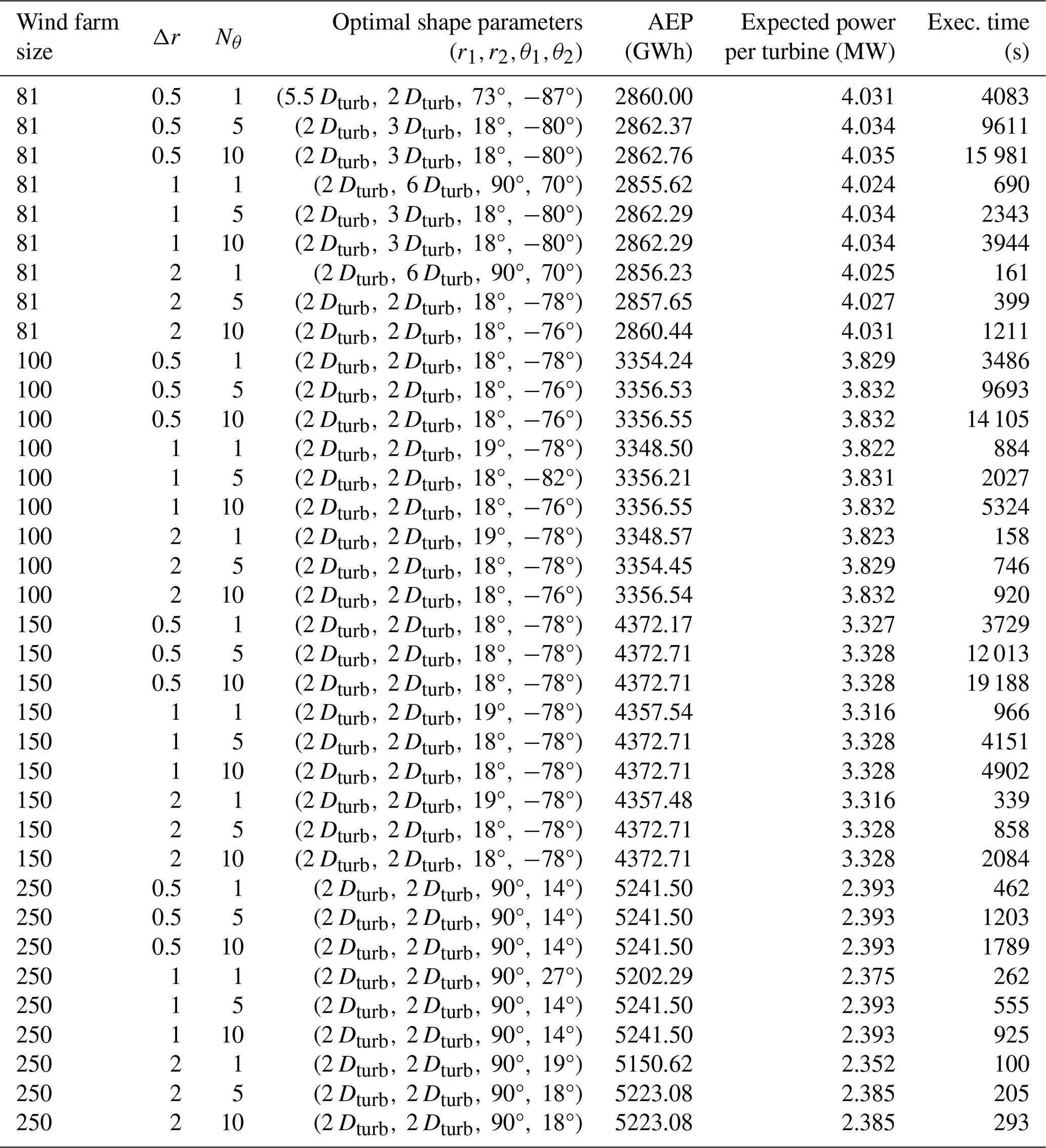
Table 3 Optimal AEP, shape configuration, and mean power per turbine for an increasing number of turbines.

Figure 5 Best layouts for wind farm sizes of 81, 100, 150, and 250 turbines, displayed in panels (a), (b), (c), and (d) respectively, using Algorithm 1.

6 Exploration method's impact on the AEP

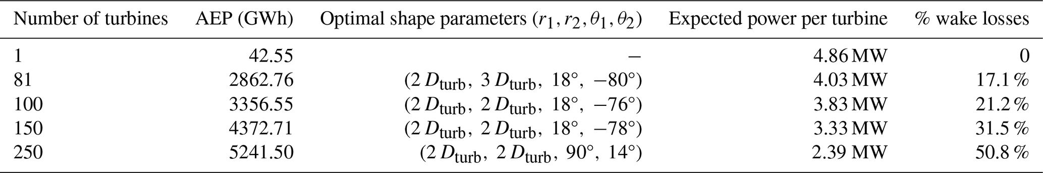
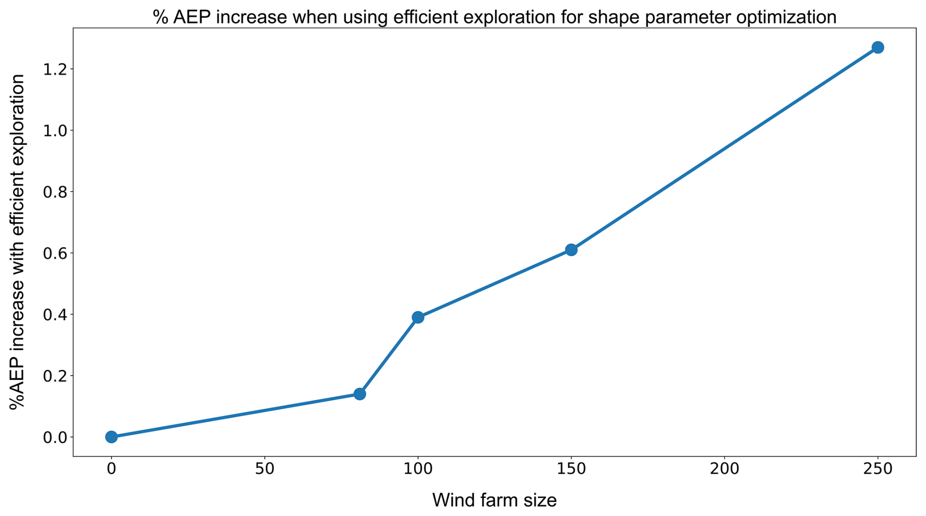
The optimization layout algorithm presented in this paper relies on the discrete exploration of the space of shape parameters $(r_{\mathrm{1}},r_{\mathrm{2}},{\mathit{\theta }}_{\mathrm{1}},{\mathit{\theta }}_{\mathrm{2}})\in [D_{min},D_{max}{]}^{\mathrm{2}}\times [-\mathit{\pi }/\mathrm{2},\mathit{\pi }/\mathrm{2}{]}^{\mathrm{2}}$. Despite the angles' search space reduction technique presented in Sect. 4.2 and Algorithm A2, exploring this space using fine discretization is numerically too demanding since it requires running step 4 of Algorithm 1 for a number of shape parameters too large for a reasonable running time. Unfortunately, the performance of the optimization depends on the capacity to tune the shape parameters finely. Achieving such a fine-tuning with Algorithm 1 requires using a small shape-parameter space discretization step. Therefore, there is a strong incentive to develop heuristic methods to explore the shape parameters' space other than by using the angle search space reduction associated with a brute-force-like exploration method. Indeed, using more efficient shape-parameter-space exploration methods allows for a good trade-off between a fine-tuning of these parameters and a reasonable computation time. In this section, we present optimization results using such a heuristic to provide a benchmark for an aligned optimization algorithm. Unfortunately, for industrial confidentiality reasons, we do not describe its principle and only focus on the improvement in terms of AEP. Again, we have run the optimization procedure for wind farms of 81, 100, 150, and 250 turbines. The results in terms of optimal shape parameters, AEP, expected power per turbine, and wake losses are summarized in Table 4, and the optimal layouts are displayed in Fig. 6. The optimal layout obtained using this heuristic exhibits the same behavior as those found in the previous section regarding r₁ and r₂. Indeed, these parameters are systemically found to be equal to the lowest possible value. In contrast, the optimal angles are not the same. One of the alignment directions is conserved (≈18°), but the other one is quite different even when taking into account the 180° periodicity of the angles. Concerning the AEP, using a heuristic to explore the space of shape parameters more efficiently allows for improvement. Interestingly, as illustrated in Fig. 7 and in the last column of Table 4, the percentage of AEP increase grows almost linearly concerning the wind farm size and reaches 1 % for the larger one. This behavior stems from the decreasing degrees of freedom in the turbine's optimal placing problem as the wind farm size grows. Therefore, for larger farms, the efficiency of the shape parameters' optimization algorithm is of greater importance than for smaller farms; thus, there is a more substantial improvement in AEP for large farms when using a better exploration algorithm for the space of shape parameters. These results prove to be a strong incentive to develop efficient heuristics to explore the space of shape parameters.

Table 4 Optimal AEP, shape configuration, and mean power per turbine for an increasing number of turbines using a fast heuristic for the optimization of the shape's parameters.

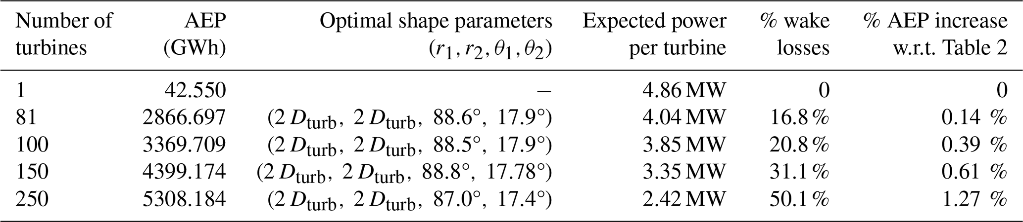
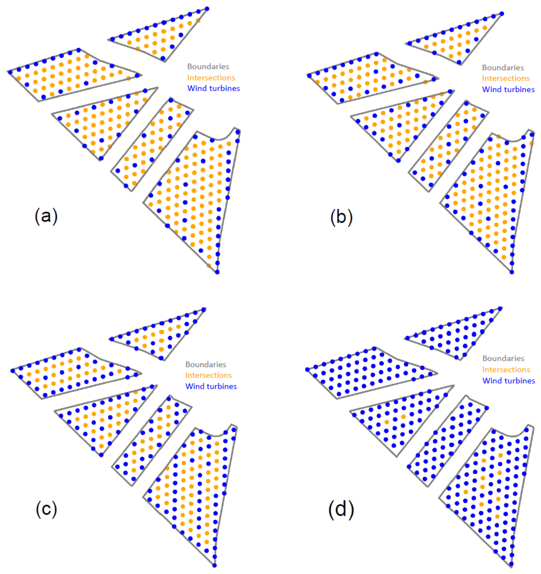
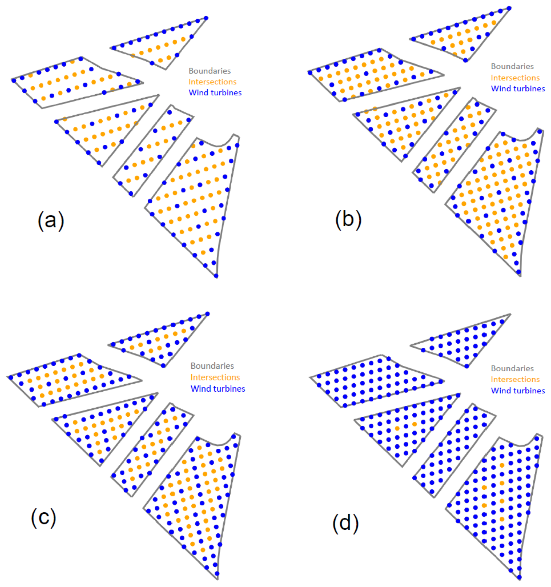
Figure 6 Best layouts for wind farm sizes of 81, 100, 150, and 250 turbines, displayed in panels (a), (b), (c), and (d) respectively, using an efficient shape parameter exploration method and the same local-search algorithm.

Figure 7 Percentage of AEP increase when using an efficient shape-parameter-space exploration method compared to the brute force discretization from Algorithm 1.

7 Conclusions

This work tackles the wind farm layout optimization problem with alignment constraints. We introduced a model of the corresponding optimization problem and adapted the DEBO algorithm from Thomas et al. (2023) to this new problem. The proposed method is based on an exploration heuristic for computing the grid parameters and a local-search method to place the turbines on the grid's intersections optimally. We have shown that this method performs well on the benchmark of IEA Wind Task 37 (Thomas, 2022) since it produced an AEP increase of 0.41 % compared to the baseline layout, even though the latter does not satisfy any alignment constraints and is potentially less prone to significant wake losses. Using this numerical example, we have also demonstrated the benefits of developing efficient heuristics for exploring the grid parameters. Indeed, using efficient heuristics allows for a better trade-off between wake-loss reduction and computation time. Therefore, these heuristics can be used to find layouts with higher AEP or to use more precise and computationally demanding AEP models. A more efficient algorithm can enable the introduction of other optimization parameters or constraints, such as cable routing or shared mooring for floating farms. Otherwise, to quantify the effect of alignment constraints on the wake losses, one could perform a sensitivity analysis by allowing small displacements of each turbine, resulting in an almost aligned layout. Finally, future works can also investigate the robustness of the optimal layout with respect to the wind probability measure ${\mathbb{P}}_{\mathrm{W}}:={\sum }_{n=\mathrm{1}}^{N_{\mathrm{W}}}p(w_{\mathrm{s}}^n,w_{\mathrm{d}}^n)\mathit{\delta }(w_{\mathrm{s}}^n,w_{\mathrm{d}}^n)$. The sensitivity of the AEP with respect to the wind probability is easy to estimate if the support of the probability is unchanged, i.e., if the modified probability ${\widehat{\mathbb{P}}}_{\mathrm{W}}$ is ${\widehat{\mathbb{P}}}_{\mathrm{W}}:={\sum }_{n=\mathrm{1}}^{N_{\mathrm{W}}}\left[p(w_{\mathrm{s}}^n,w_{\mathrm{d}}^n)+\mathrm{\Delta }p(w_{\mathrm{s}}^n,w_{\mathrm{d}}^n)\right]\mathit{\delta }(w_{\mathrm{s}}^n,w_{\mathrm{d}}^n)$, with $\sum \mathrm{\Delta }p(w_{\mathrm{s}}^n,w_{\mathrm{d}}^n)=\mathrm{0}$. In this case we have

$$\mathrm{\Delta }\mathrm{AEP}\left({\mathbf{F}}_n\right):=\mathrm{8760}\sum _{n=\mathrm{1}}^{N_{\mathrm{W}}}\mathcal{P}({\mathbf{F}}_n,w_{\mathrm{s}}^n,w_{\mathrm{d}}^n)\mathrm{\Delta }p(w_{\mathrm{s}}^n,w_{\mathrm{d}}^n)).$$

However, when the probability's support is also varying, computations are much more involved, and future works could focus on using distributionally robust optimization methods (see Rahimian and Mehrotra, 2022, for a review on the subject) to produce robust layouts with respect to the wind probability measure.

Appendix A: Algorithms in pseudo-code

Algorithm A1 GenerateR1R2$(\mathrm{\Delta }r,D_{min},D_{max})$.

1:

$R_{\mathrm{1},\mathrm{2}}\leftarrow \mathrm{\varnothing }$

2:

$r_{\mathrm{1}}\leftarrow D_{min}.D_{\mathrm{turb}}$

3:

angles←∅

4:

while $r_{\mathrm{1}}\le D_{max}.D_{\mathrm{turb}}$ do

5:

$r_{\mathrm{2}}\leftarrow D_{min}.D_{\mathrm{turb}}$

6:

while $r_{\mathrm{2}}\le D_{max}.D_{\mathrm{turb}}$ do

7:

$R_{\mathrm{1},\mathrm{2}}\leftarrow R_{\mathrm{1},\mathrm{2}}\cup \left\{r_{\mathrm{1}},r_{\mathrm{2}})\right\}$

8:

$r_{\mathrm{2}}\leftarrow r_{\mathrm{2}}+\mathrm{\Delta }r$

9:

end while

10:

$r_{\mathrm{1}}\leftarrow r_{\mathrm{1}}+\mathrm{\Delta }r$

11:

end while

12:

return  R_1,2

Algorithm A2 ReduceSearchSpace$(R_{\mathrm{1},\mathrm{2}},\mathrm{\Delta }\mathit{\theta },D_{min},D_{max}$, D_turb,N_θ).

1:

Θ←∅

2:

for $(r_{\mathrm{1}},r_{\mathrm{2}})\in R_{\mathrm{1},\mathrm{2}}$ do

3:

${\mathrm{\Theta }}_{r_{\mathrm{1}},r_{\mathrm{2}}}\leftarrow$ GetBestAngles$(r_{\mathrm{1}},r_{\mathrm{2}},\mathrm{\Delta }\mathit{\theta },D_{min},D_{max},D_{\mathrm{turb}},N_{\mathit{\theta }})$

4:

$\mathrm{\Theta }\leftarrow \mathrm{\Theta }\cup {\mathrm{\Theta }}_{r_{\mathrm{1}},r_{\mathrm{2}}}$

5:

end for

6:

return  Θ

Algorithm A3 GetBestAngles$(r_{\mathrm{1}},r_{\mathrm{2}},\mathrm{\Delta }\mathit{\theta },D_{min},D_{max},D_{\mathrm{turb}}$, N_θ).

1:

farms←∅

2:

${\mathrm{\Theta }}_{r_{\mathrm{1}},r_{\mathrm{2}}}\leftarrow \mathrm{\varnothing }$

3:

${\mathit{\theta }}_{\mathrm{1}}\leftarrow -\frac{\mathit{\pi }}{\mathrm{2}}+\mathrm{\Delta }\mathit{\theta }$

4:

while ${\mathit{\theta }}_{\mathrm{1}}\le \frac{\mathit{\pi }}{\mathrm{2}}$ do

5:

${\mathit{\theta }}_{\mathrm{2}}\leftarrow -\frac{\mathit{\pi }}{\mathrm{2}}$

6:

while ${\mathit{\theta }}_{\mathrm{2}}\le {\mathit{\theta }}_{\mathrm{1}}-\mathrm{\Delta }\mathit{\theta }$ do

7:

$D_{\mathrm{grid}}\leftarrow {min}_{\mathit{z}\in {\mathbb{Z}}_{*}^{\mathrm{2}}}∥P_{{\mathcal{B}}_{\mathrm{0}}}^{\mathcal{B}({\mathit{\theta }}_{\mathrm{1}},{\mathit{\theta }}_{\mathrm{2}},r_{\mathrm{1}},r_{\mathrm{2}})}z∥$

8:

if $\left(D_{\mathrm{grid}}\ge D_{min}.D_{\mathrm{turb}}\right)\wedge \left({\mathit{\theta }}_{\mathrm{1}}-{\mathit{\theta }}_{\mathrm{2}}\le \mathit{\pi }-\mathrm{\Delta }\mathit{\theta }\right)$  then

9:

n←1

10:

for i=0 to i=1  do

11:

for j=0 to j=1  do

12:

${\mathbf{F}}_{\mathrm{4}}\left(n\right)\leftarrow P_{{\mathcal{B}}_{\mathrm{0}}}^{\mathcal{B}({\mathit{\theta }}_{\mathrm{1}},{\mathit{\theta }}_{\mathrm{2}},r_{\mathrm{1}},r_{\mathrm{2}})}\left(\begin{array}{c}i\\ j\end{array}\right)$

13:

$n\leftarrow n+\mathrm{1}$

14:

end for

15:

end for

16:

$\mathrm{aep}\leftarrow {\mathbb{E}}_{\mathrm{W}}\left[\mathcal{P}({\mathbf{F}}_{\mathrm{4}},w_{\mathrm{s}},w_{\mathrm{d}})\right]$

17:

$\mathrm{farms}\leftarrow \mathrm{farms}\cup \left\{({\mathit{\theta }}_{\mathrm{1}},{\mathit{\theta }}_{\mathrm{2}},\mathrm{aep})\right\}$

18:

end if

19:

${\mathit{\theta }}_{\mathrm{2}}\leftarrow {\mathit{\theta }}_{\mathrm{2}}+\mathrm{\Delta }\mathit{\theta }$

20:

end while

21:

${\mathit{\theta }}_{\mathrm{1}}\leftarrow {\mathit{\theta }}_{\mathrm{1}}+\mathrm{\Delta }\mathit{\theta }$

22:

end while

23:

sort(farms) {by decreasing order of aep}

24:

for i=1 to i=N_θ do

25:

${\mathrm{\Theta }}_{r_{\mathrm{1}},r_{\mathrm{2}}}\leftarrow {\mathrm{\Theta }}_{r_{\mathrm{1}},r_{\mathrm{2}}}\cup \left\{\left(\mathrm{farms}\right(i).{\mathit{\theta }}_{\mathrm{1}},\mathrm{farms}(i).{\mathit{\theta }}_{\mathrm{2}})\right\}$

26:

end for

27:

return  ${\mathrm{\Theta }}_{r_{\mathrm{1}},r_{\mathrm{2}}}$

Algorithm A4 GenerateConfigs$(R_{\mathrm{1},\mathrm{2}},\mathrm{\Theta },D_{min},D_{max},D_{\mathrm{turb}})$.

1:

grids←∅

2:

for  $(r_{\mathrm{1}},r_{\mathrm{2}})\in R_{\mathrm{1},\mathrm{2}}$ do

3:

for $({\mathit{\theta }}_{\mathrm{1}},{\mathit{\theta }}_{\mathrm{2}})\in \mathrm{\Theta }$ do

4:

$D_{\mathrm{grid}}\leftarrow {min}_{\mathit{z}\in {\mathbb{Z}}_{*}^{\mathrm{2}}}∥P_{{\mathcal{B}}_{\mathrm{0}}}^{\mathcal{B}({\mathit{\theta }}_{\mathrm{1}},{\mathit{\theta }}_{\mathrm{2}},r_{\mathrm{1}},r_{\mathrm{2}})}z∥$

5:

if ${min}_{\mathit{z}\in {\mathbb{Z}}_{*}^{\mathrm{2}}}∥P_{{\mathcal{B}}_{\mathrm{0}}}^{\mathcal{B}({\mathit{\theta }}_{\mathrm{1}},{\mathit{\theta }}_{\mathrm{2}},r_{\mathrm{1}},r_{\mathrm{2}})}z∥\ge D_{min}.D_{\mathrm{turb}}$ then

6:

$\mathrm{grids}\leftarrow \mathrm{grids}\cup \mathit{\left\{}\right(r_{\mathrm{1}},r_{\mathrm{2}},{\mathit{\theta }}_{\mathrm{1}},{\mathit{\theta }}_{\mathrm{2}}\left)\mathit{\right\}}$

7:

end if

8:

end for

9:

end for

10:

return  grids

Algorithm A5 ComputeAllIntersections(grids, D_min, Ω).

1:

intersections_sets←{∅}

2:

n←1

3:

while  n≤card(grids)  do

4:

{Compute basic shape vector}

5:

$r_{\mathrm{1}},r_{\mathrm{2}},{\mathit{\theta }}_{\mathrm{1}},{\mathit{\theta }}_{\mathrm{2}}\leftarrow \mathrm{grids}\left(n\right)$

6:

$v_{\mathrm{1}}\leftarrow \left(r_{\mathrm{1}}\cos \right({\mathit{\theta }}_{\mathrm{1}}),r_{\mathrm{1}}\sin ({\mathit{\theta }}_{\mathrm{1}}\left)\right)$

7:

$v_{\mathrm{2}}\leftarrow \left(r_{\mathrm{2}}\cos \right({\mathit{\theta }}_{\mathrm{2}}),r_{\mathrm{2}}\sin ({\mathit{\theta }}_{\mathrm{2}}\left)\right)$

8:

{Function of the intersections}

9:

$I_{v_{\mathrm{1}},v_{\mathrm{2}}}({\mathrm{\Delta }}_{\mathrm{1}},{\mathrm{\Delta }}_{\mathrm{2}}):=\mathit{\{}{k}_{\mathrm{1}}{v}_{\mathrm{1}}+k_{\mathrm{2}}{v}_{\mathrm{2}}\in {\mathbb{Z}}^{\mathrm{2}}\mathrm{s}.\mathrm{t}.\left[k_{\mathrm{1}}{v}_{\mathrm{1}}+k_{\mathrm{2}}{v}_{\mathrm{2}}+({\mathrm{\Delta }}_{\mathrm{1}},{\mathrm{\Delta }}_{\mathrm{2}})\right]\in \mathrm{\Omega };(k_{\mathrm{1}},k_{\mathrm{2}})\in {\mathbb{Z}}^{\mathrm{2}}\mathit{\}}$

10:

{Compute offset maximising the number of admissible intersections}

11:

$({\mathrm{\Delta }}_{\mathrm{1}}^{*},{\mathrm{\Delta }}_{\mathrm{2}}^{*})\leftarrow \arg {max}_{{\mathrm{\Delta }}_{\mathrm{1}},{\mathrm{\Delta }}_{\mathrm{2}}\in [\mathrm{0},\mathrm{1}{)}^{\mathrm{2}}}\mathrm{card}\left(I_{v_{\mathrm{1}},v_{\mathrm{2}}}\right({\mathrm{\Delta }}_{\mathrm{1}},{\mathrm{\Delta }}_{\mathrm{2}}\left)\right)$

12:

{Add intersections to the set of intersections}

13:

if card($I_{v_{\mathrm{1}},v_{\mathrm{2}}}({\mathrm{\Delta }}_{\mathrm{1}}^{*},{\mathrm{\Delta }}_{\mathrm{2}}^{*}))\ge N_{max}$ then

14:

$\mathrm{intersections}\mathit{\_}\mathrm{sets}\leftarrow \left\{\left(I_{v_{\mathrm{1}},v_{\mathrm{2}}}({\mathrm{\Delta }}_{\mathrm{1}}^{*},{\mathrm{\Delta }}_{\mathrm{2}}^{*}),(r_{\mathrm{1}},r_{\mathrm{2}},{\mathit{\theta }}_{\mathrm{1}},{\mathit{\theta }}_{\mathrm{2}})\right)\right\}$ ⋃intersections_sets

15:

end if

16:

$n\leftarrow n+\mathrm{1}$

17:

end while

18:

return  intersections_sets

Algorithm A6 GreedyInitialization(intersections).

1:

$(x_{\mathrm{0}},y_{\mathrm{0}})\leftarrow \arg {max}_{x,y}\mathit{\{}x-y\mathrm{s}.\mathrm{t}.(x,y)\in \mathrm{intersections}\mathit{\}}$

2:

F₁(1)←(x₀  y₀)

3:

n_t←1

4:

intersections ← intersections∖{(x₀  y₀)}

5:

while $n_t<N_{max}$ do

6:

$(x^{*}{y}^{*}{)}^{\top }\leftarrow \arg {max}_{(x,y)\in \mathrm{intersections}}{\mathbb{E}}_{\mathrm{W}}$ $\left\{\mathcal{P}\left({\mathbf{F}}_{n_t}\oplus \left(xy\right),w_{\mathrm{s}},w_{\mathrm{d}}\right)\right\}$

7:

${\mathbf{F}}_{n_t+\mathrm{1}}\leftarrow {\mathbf{F}}_{n_t}\oplus \left(x^{*}{y}^{*}\right)$

8:

$n_t\leftarrow n_t+\mathrm{1}$

9:

intersections ← intersections $\setminus \mathit{\left\{}\right(x^{*}{y}^{*}\left)\mathit{\right\}}$

10:

end while

11:

return  ${\mathbf{F}}_{N_{max}}$

Algorithm A7 LocalSearch$({\mathbf{F}}_{N_{max}},\mathrm{intersections})$.

1:

convergence $\leftarrow \perp$

2:

$\mathrm{aep}\leftarrow {\mathbb{E}}_{\mathrm{W}}\left\{\mathcal{P}({\mathbf{F}}_{N_{max}},w_{\mathrm{s}},w_{\mathrm{d}})\right\}$

3:

while ¬ convergence do

4:

${\mathbf{H}}_{N_{max}}\leftarrow {\mathbf{F}}_{N_{max}}$

5:

random_indices ← shuffle($\left[\right[\mathrm{0},\mathrm{\dots },N_{max}\left[\right[$)

6:

for indice ∈ random_indices do

7:

{compute all possible layouts by moving ith turbine}

8:

children_layout ← generate_children(${\mathbf{F}}_{N_{max}}$, indice, intersections)

9:

for $({\mathbf{G}}_{N_{max}},{\mathrm{intersections}}_G)\in$children_layout  do

10:

if ${\mathbb{E}}_{\mathrm{W}}\left\{\mathcal{P}({\mathbf{G}}_{N_{max}},w_{\mathrm{s}},w_{\mathrm{d}})\right\}>\mathrm{aep}$ then

11:

${\mathbf{F}}_{N_{max}}\leftarrow {\mathbf{G}}_{N_{max}}$

12:

$\mathrm{aep}\leftarrow {\mathbb{E}}_{\mathrm{W}}\left\{\mathcal{P}({\mathbf{F}}_{N_{max}},w_{\mathrm{s}},w_{\mathrm{d}})\right\}$

13:

intersections←intersections_G

14:

end if

15:

end for

16:

end for

17:

convergence $\leftarrow {\mathbf{F}}_{N_{max}}={\mathbf{H}}_{N_{max}}$

18:

end while

19:

return  $\left({\mathbf{F}}_{N_{max}},\mathrm{aep}\right)$

Algorithm A8 generate_children$({\mathbf{F}}_{N_{max}},\mathrm{indice},\mathrm{intersections})$.

1:

children_layout ←∅

2:

for (x  y)∈ intersections do

3:

${\mathbf{G}}_{N_{max}}\leftarrow {\mathbf{F}}_{N_{max}}$

4:

intersection_G← intersections

5:

$\left(x_{\mathrm{new}}{y}_{\mathrm{new}}\right)\leftarrow {\mathbf{G}}_{N_{max}}\left(\mathrm{indice}\right)$

6:

${\mathbf{G}}_{N_{max}}\left(\mathrm{indice}\right)\leftarrow \left(xy\right)$

7:

intersections_G← intersections${}_G\setminus \mathit{\left\{}\right(xy\left)\mathit{\right\}}\cup \mathit{\left\{}\right(x_{\mathrm{new}},y_{\mathrm{new}}\left)\mathit{\right\}}$

8:

children_layout ← children_layout $\cup \mathit{\left\{}\right({\mathbf{G}}_{N_{max}},{\mathrm{intersections}}_G\left)\mathit{\right\}}$

9:

end for

10:

return  children_layout

Algorithm A9 PlaceTurbines(intersections).

1:

${\mathbf{F}}_{N_{max}}\leftarrow$ GreedyInitialization(intersections)

2:

$\left({\mathbf{F}}_{N_{max}},\mathrm{aep}\right)\leftarrow$ LocalSearch$({\mathbf{F}}_{N_{max}},\mathrm{intersections})$

3:

return  $\left({\mathbf{F}}_{N_{max}},\mathrm{aep}\right)$