Offshore wind farm layout optimization accounting for participation in secondary reserve markets

Wind farm layout optimization usually aims at maximizing annual energy production by placing wind turbines in a strategic way to avoid wake losses. However, this might not lead to optimal profits because of the volatility of electricity prices. Moreover, with the growing unpredictability and variability of future power systems due to the increase in renewable electricity production, wind farm operators will have a more important role in balancing the system through participation in reserve markets. This study presents a new formulation for wind farm layout optimization where the objective function aims at maximizing revenues from both day-ahead and reserve markets. It uses stochastic gradient descent for the optimization and probabilistic forecasts for wind power and electricity prices. The new formulation is applied to a test case based on a real-life offshore wind farm in Belgium. An important conclusion is that annual revenues are expected to increase in a significant way when accounting for participation in reserve markets, while exhibiting a lower supplied energy production. Moreover, layouts optimized for revenue maximization with reserve participation tend to show better yearly revenues than when considering the day-ahead market only in the objective function. Expected revenues are also higher by 0.18 % on average for the new methodology than when using the maximization of annual energy production, widely used in the literature, as the objective function.

1 Introduction

With the sharp increase in renewable energy sources in modern power systems, balancing electrical load and generation throughout the day is becoming a challenge. In the case of a real-time imbalance in the system, the transport system operator (TSO) needs to activate reserves in order to restore the balance and avoid frequency deviations. In the near future, with a high penetration of weather-dependent electricity generation, the intra-hour variability and randomness will become more significant, increasing the need for fast regulation and the value of reserve. Reserve markets, which allow power plant operators to act as a balancing service provider (BSP), will be critical for the reliable integration of renewable electricity. Because offshore wind generation capacity is expected to grow steadily in the future, wind farm operators will have an important role in reserve markets and system balancing. Allowing offshore wind farms to participate in the reserve market will be of mutual interest to TSOs and wind producers. Moreover, it has been proven that modern wind turbines with variable rotation speed have intrinsic fast ramping-down and ramping-up capabilities, which can be effectively used to provide ancillary services (Kayedpour et al., 2024, 2022). Ramping down is virtually done at no cost (if prices for down reserve are favourable), and ramping up is subject to the availability of wind power. To alleviate frequency deviations, the TSO has several reserve capacities, with different requirements for maximum ramping and activation time. The focus of this work will be on automatic frequency reserve restoration (aFRR), also called secondary reserve or R2. Indeed, volume needs of secondary reserves are usually higher and are expected to reach even larger values than those for primary reserve in the future (Elia, 2023). Moreover, primary reserve requires an activation and ramping to full capacity within seconds (Perroy et al., 2020), which might be prohibitive within wind farms, where wind and wake effects take time to propagate. Tertiary reserve is manually activated and is only used to complement and release secondary reserve (e.g. for very extensive imbalances). It must be able to stay active for a long period of time (hours), which could be a challenge for wind farm operators because of the variability of wind. Therefore, secondary reserves seem to be suitable for increasing revenues of wind farms participating in reserve markets (Sumetha-Aksorn et al., 2022; Windvision et al., 2015). Secondary reserves have a fast response time, are used in both directions to restore a frequency of 50 Hz, and remain active as long as necessary. The TSO activates aFRR automatically by sending a set point every 4 s, and the requested energy is to be activated within 7.5 to 15 min in the case of selection of the full volume of the aFRR energy bid. In Belgium, the volume need for upward aFRR determined by the TSO was 117 MW in 2023 (Elia, 2023). Regarding other European countries, in France, the TSO has prescribed a daily average of 709 MW of aFRR to French stakeholders (ENTSO-E, 2024). In the Netherlands, the determined dimensioning minimum of upward aFRR was 324 MW in 2023. The Nordic upward aFRR capacity market (which covers eastern Denmark, Sweden, Finland, and Norway) has a volume need of 300 MW. However, those needs are expected to increase in the future. For example, in Denmark, for the west bidding zone DK1, the current upward aFRR need is 100 MW, but it is expected to reach up to 194 MW in 2035 and 298 MW by 2040 (Energinet, 2023).

Regarding the participation of wind farms in a joint day-ahead energy and reserve market (JERM), optimal offering and allocation policies have been investigated, but with the assumption of constant electricity prices (Soares et al., 2017). This does not capture the variation of day-ahead and reserve prices with wind speed and wind direction. A combined energy and regulation reserve market model has been developed to encourage wind producers to regulate their short-term outputs (Liang et al., 2011), but it assumes that marginal revenues of providing day-ahead energy are always higher than the marginal revenues for upward reserve as well as perfect forecasts of market prices. Provision of reserve by wind power units has been considered for generation capacity expansion (Cañas-Carretón and Carrión, 2020) and simulations were only carried out over 9 representative days of load and generation.

While current wind farms have usually been designed to maximize their power output, future wind farms should be planned and built taking into account the participation in reserve markets, especially if the size of the latter becomes more significant. Wind farm layout optimization (WFLO) generally aims at maximizing annual energy production (AEP). It attempts to choose the best placement for turbines, which is equivalent to minimizing wake losses. Indeed, when wind turbines extract mechanical energy from the wind to produce electricity, they cause a reduction of wind speed behind them. Downstream turbines in the wake therefore produce less energy. On a site with specific wind conditions, WFLO will avoid aligning a turbine in the directions of dominant wind. Layout optimization for maximizing AEP has been widely studied in the literature, using gradient-based optimization techniques (Quick et al., 2023; Valotta Rodrigues et al., 2024; Park and Law, 2015), gradient-free techniques (Hou et al., 2015; Feng and Shen, 2015; Long et al., 2020), or comparing both (Thomas et al., 2023). The idea behind maximizing AEP is that it will maximize profits for wind farm operators selling energy on the day-ahead energy market (DAEM). However, both objectives might not lead to the same results because of the high volatility of electricity prices. Producing too much energy in periods of low prices will lead to reduced profits. When considering only the day-ahead market, if patterns of low and high prices do not match wind direction patterns, optimizing AEP is not the same as maximizing profit. Indeed, maximizing profit might lead to higher profits while decreasing supplied energy (and thus turbine loads). WFLO for yearly profit has been studied in previous works (Stanley et al., 2021; González et al., 2010; Gonzalez et al., 2012), but wind power was sold only on the day-ahead market. Adding participation in the reserve market will also impact results if day-ahead (DA) and reserve prices do not show the same variations with regard to wind direction.

To the best of the authors' knowledge, this is the first paper that presents a wind farm layout optimization that accounts for participation in reserve markets in the revenue objective function. Therefore, the main contribution of this paper is the formulation of a new objective function for the wind farm layout optimization problem. The latter allows taking into account the participation in reserve markets during the design process. The new objective function aims at maximizing expected yearly revenues of a wind farm participating in both day-ahead and secondary upward reserve markets. It allows computing the optimal offering in both markets, the reserve allocation strategy, and subsequent expected revenues. The new objective function considers the uncertainty in forecasts of wind power, electricity prices, and activated reserve volumes. The estimated penalties and balancing costs for failing to provide energy and reserve are also taken into account. The study is conducted for the Belgian system using existing market rules. However, although this system has some peculiarities, the main methodology could be applied in other systems with minor modifications.

Because computing yearly revenues at each iteration step of the optimization is too costly, stochastic gradient descent (SGD) is used. This prompts the need to make the revenue function differentiable. The gradient of the total revenue is estimated for a limited number of time steps: this approach enables accurate results with reasonable computation time. The new formulations are applied on a real wind farm using historical data for wind and electricity prices. When considering the current built layout, it is shown that operating the wind farm with provision of reserve leads to significantly higher yearly revenues than when participating only in DAEM. Then, the new WFLO methodology is applied to optimize the layout while accounting for reserve participation. Yearly revenues, supplied energy, and AEP of the best optimized layout are compared with regard to the current built configuration of the test wind farm. The optimized layout is also compared with those obtained using the traditional AEP maximization formulation. A revenue function only accounting for participation in the day-ahead market is also used for the optimization. The three approaches are compared in terms of expected yearly revenues and supplied energy. Finally, generalization to unseen data is studied.

The remainder of the paper is structured as follows. In Sect. 2, the general formulation for the computation for revenues from both day-ahead and reserve markets is presented, as well as its integration in the wind farm layout optimization problem. Section 3 details the wind farm optimization test case and briefly explores historical data from Belgium. Section 4 analyses results and comparisons are made with more traditional wind farm layout optimization formulations. Finally, conclusions and future work are gathered in the last section.

2 Methods

A total of 1 d before real-time delivery (market closure is at noon), for each time step t of the 24 h of the next day k, a wind farm operator does the following:

• forecasts available wind power ${\widehat{P}}_{k,t}^{\text{wind,\hspace{0.17em}avail}}$

• decides the total amount of power sold to both day-ahead and reserve markets $P_{k,t}^{\mathrm{c}}$

• decides the amount of reserve capacity to procure to the reserve market $R_{k,t}={\mathit{\alpha }}_{k,t}\cdot P_{k,t}^{\mathrm{c}}$

• computes the power to be sold in the day-ahead energy market $P_{k,t}^{\text{DA}}=P_{k,t}^{\mathrm{c}}-{\widehat{R}}_{k,t}$

The wind farm reserve capacity represents the amount of power that the wind farm holds back from electricity production to sell in the reserve market instead of the day-ahead energy market. Based on weather forecasts (and thus wind power forecasts), a wind farm operator bids its electricity production in the day-ahead market and the reserve capacity in the secondary reserve market. On the day of delivery, the wind farm must be able to supply both the day-ahead and activated reserve quantities. In this work, it is assumed that wind farms always prioritize providing reserve (as the wind farm is contractually bound to reserve this capacity).

The accuracy of weather and thus wind power forecasts is crucial in order to make relevant bids in both markets: underestimation leads to lower bids and decreased revenues, while overestimating production results in inability to supply contracted bids, thus incurring financial penalties. Moreover, electricity prices can be highly volatile, and the actual activation of reserve depends on the system imbalance, which is also fluctuating. Forecast errors in electricity prices and activation volume can lead to a wrong estimation of expected revenue. In this work, we assume that forecast errors follow a Gaussian distribution with a given mean and standard deviation. For each considered time step, S forecast errors are randomly sampled using a Monte Carlo approach.

2.1 Wind power forecasts

The forecast of available wind power ${\widehat{P}}_{k,t}^{\text{wind,\hspace{0.17em}avail}}$ depends on (previously) forecasted free-flow wind speed ${\widehat{u}}_{k,t}^{\mathrm{\infty }}$ and wind direction ${\widehat{\mathit{\theta }}}_{k,t}$.

$${\widehat{P}}_{k,t,s}^{\text{wind,\hspace{0.17em}avail}}=f({\widehat{u}}_{k,t,s}^{\mathrm{\infty }},{\widehat{\mathit{\theta }}}_{k,t,s})$$

The operator f(⋅) denotes the conversion of wind data to wind power: it is based on the wind turbine power curve and should account for wake effects arising within the wind farm. The index s denotes the Monte Carlo sample number related to forecast error sampling.

The forecasted wind speed ${\widehat{u}}_{k,t}^{\mathrm{\infty }}$ is derived from the actual realization of wind speed and a forecast error sampled from a normal distribution.

$$\begin{array}{}\text{(1)}& \begin{array}{rl}{\widehat{u}}_{k,t,s}^{\mathrm{\infty }}& =u_{k,t}^{\mathrm{\infty }}+{\mathit{ϵ}}_{k,t,s}^u\\ {\mathit{ϵ}}_{k,t,s}^u& \sim N(\mathrm{0},{\mathit{\sigma }}^u)\end{array}\end{array}$$

The same process is used to forecast wind direction

$$\begin{array}{}\text{(2)}& \begin{array}{rl}{\widehat{\mathit{\theta }}}_{k,t,s}^{\mathrm{\infty }}& ={\mathit{\theta }}_{k,t}^{\mathrm{\infty }}+{\mathit{ϵ}}_{k,t,s}^{\mathit{\theta }}\\ {\mathit{ϵ}}_{k,t,s}^{\mathit{\theta }}& \sim N(\mathrm{0},{\mathit{\sigma }}^{\mathit{\theta }})\end{array}\end{array}$$

Therefore, forecasts of available wind power can be written as

$$\begin{array}{}\text{(3)}& {\widehat{P}}_{k,t,s}^{\text{avail}}=f_P(u_{k,t}^{\mathrm{\infty }}+{\mathit{ϵ}}_{k,t,s}^u,{\mathit{\theta }}_{k,t}^{\mathrm{\infty }}+{\mathit{ϵ}}_{k,t,s}^{\mathit{\theta }})+{\mathit{ϵ}}_{k,t,s}^{f_P}.\end{array}$$

${\mathit{ϵ}}_{k,t,s}^{f_P}$ is the modelling error associated with the wind farm model. For wind speed forecasting, literature shows that forecast errors follow a Gaussian distribution with mean 0 and standard deviation approximately equal to 15 % (ECMWF, 2024). For wind direction, day-ahead forecasts show a root mean squared error of 4.2° (Chitsazan et al., 2019). In real life, the operator should first forecast wind speed (the day-ahead prediction of wind speed is widely studied in the literature) and wind direction, then obtain the corresponding wind power forecast by converting this wind information to power using a wind power model.

2.2 Day-ahead energy market

The day-ahead energy market is a financial market where participants purchase and sell electrical energy at financially binding day-ahead prices for the following day. Electricity is traded at 12:00 LT for the 24 h of the next day and the market is cleared based on an auction mechanism, where market price and volume represent the intersection point between the demand and supply curves. After the auctions on day-ahead markets are closed, existing shortfalls or surpluses can still be evened out through intra-day trading. However, the intra-day market is not considered in this work, as prices are extremely volatile and tend to have similar patterns as imbalance fees. Indeed, market participants are charged with imbalance fees every time they deviate from their nominations. These fees, set on a quarter-hourly basis, aim at ensuring that participants contribute efficiently to balancing the electrical system and reflect the cost related to the activation of additional energy (reserve) by the TSO.

Revenues from the day-ahead market for time step t of day k can be written as (assuming perfect forecasts)

$$\begin{array}{}\text{(4)}& {\text{Revenue}}_{k,t}^{\text{DA}}=P_{k,t}^{\text{DA}}\cdot \mathrm{\Delta }t\cdot {\mathit{\lambda }}_{k,t}^{\text{DA}}-\mathrm{\Delta }{P}_{k,t}^{\text{DA}}\cdot \mathrm{\Delta }t\cdot {\mathit{\lambda }}_{k,t}^{\text{imb}},\end{array}$$

where Δt is the duration of the time step (e.g. quarter of an hour), ${\mathit{\lambda }}_{k,t}^{\text{DA}}$ is the day-ahead price [EUR MWh⁻¹], $\mathrm{\Delta }{P}_{k,t}^{\text{DA}}$ is the contracted power not supplied, and ${\mathit{\lambda }}_{k,t}^{\text{imb}}$ is the imbalance fee [EUR MWh⁻¹].

Day-ahead prices and imbalance penalties need to be forecasted by the wind farm operator before it makes its bid on the market. For the Gaussian distribution parameters of forecast errors for day-ahead electricity prices, μ is approximately 0 and σ is around 7 % (Lago et al., 2021).

2.3 Reserve market for aFRR

Upward regulation is activated in the case of negative imbalance in the system (consumption exceeds production), and downward regulation is used for positive imbalance. In this work, we only consider the provision of upward reserve regulation since wind farms are not able to benefit from fuel-saving returns in downward regulation (Toubeau et al., 2020). Indeed, activation of downward reserves can yield both positive (the TSO pays the BSP) and negative prices (the BSP pays the TSO) (Brijs et al., 2015). Negative prices result from producers (e.g. gas-fired power plants) willing to lower their output since their energy is already sold in long-term markets and they can save operating costs: they are usually willing to pay the TSO a small amount. However, when facing scarcity of downward flexibility, BSPs may bid positive activation prices, i.e. being paid for the service, which is the only case where providing downward reserve would be profitable for wind farm operators. We assume that prices for downward reserve are usually negative, and positive prices only occur in specific conditions. It should be noted that this assumption strongly depends on market conditions, but it is suitable for the Belgian case study considered in this work. Therefore, we will only focus on upward reserve.

Revenues from the aFRR upward market are twofold. BSPs earn revenues from the procurement of reserve capacity (through capacity bids) and balancing revenues from the real-time activation of procured reserves. The reserve capacity price λ^R,c is determined through a pay-as-bid process. We assume that because of the lower production costs for wind generation than conventional power plants, capacity bids from wind farms will be well placed in the merit order and will be chosen first by the TSO. The reserve activation price λ^R,a is pay-as-cleared and contracted aFRR energy bids for possible activation on day k have to be submitted by the BSP to the TSO at the latest for the day-ahead market (day k−1). The TSO may activate aFRR energy bids partially or entirely, depending on the negative system imbalance. This process is presented in Fig. 1. The uncertainty in the balancing actions (i.e. the total amount of activated upward reserve) is modelled through scenarios of reserve activation ${\mathit{\kappa }}^{\mathrm{a}}\in [\mathrm{0},\mathrm{1}]$. Moreover, in the case of several market players bidding in the balancing market, we assume an equal distribution of reserve among all market participants.

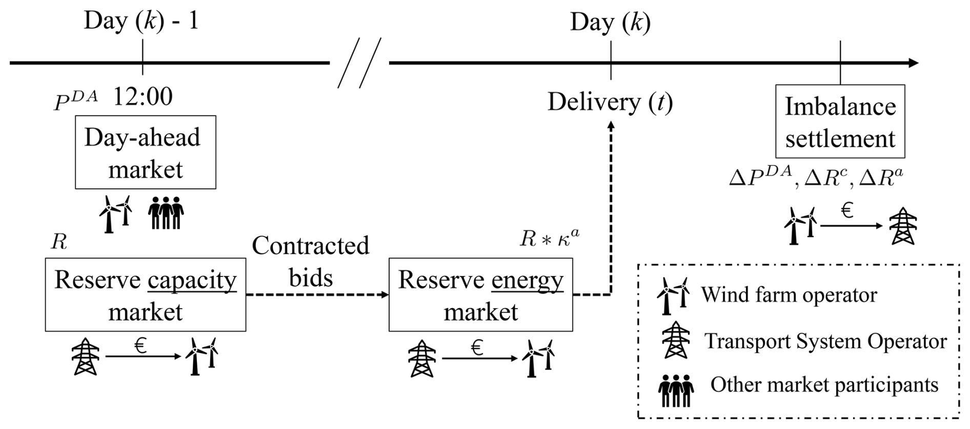
Figure 1 Bidding process of an offshore wind farm operator participating in both day-ahead and reserve markets.

Failing to provide the activated reserve requested by the TSO leads to activation penalties that are calculated as follows (Elia, 2022):

$$\begin{array}{}\text{(5)}& \begin{array}{rl}& {\text{Penalties}}_{k,t}^{\mathrm{R},\mathrm{a}}={\mathit{\gamma }}^{\mathrm{a}}\cdot {\displaystyle \frac{\text{Reserve discrepancy}}{\text{Reserve requested}}}\\ & \cdot (\text{Capacity remuneration}+\text{Activation remuneration)},\end{array}\end{array}$$

where γ^a is a penalty multiplier for failing to provide activated reserve. It is set by the TSO, and in Belgium, Elia has chosen a value of 1.3 for γ^a. The reserve discrepancy during activation (contracted reserve not supplied when requested) $\mathrm{\Delta }{R}_{k,t}^{\mathrm{a}}$ is defined as

$$\begin{array}{}\text{(6)}& \begin{array}{rl}\mathrm{\Delta }{R}_{k,t}^{\mathrm{a}}& =R_{\text{requested}}-R_{\text{supplied}}\\ \mathrm{\Delta }{R}_{k,t}^{\mathrm{a}}& =R_{k,t}\cdot {\mathit{\kappa }}_{k,t}-min(R_{k,t}\cdot {\mathit{\kappa }}_{k,t},{\widehat{P}}_{k,t}^{\text{wind,\hspace{0.17em}avail}}).\end{array}\end{array}$$

In our problem, this translates to this equation:

$$\begin{array}{}\text{(7)}& \begin{array}{rl}{\text{Penalties}}_{k,t}^{\mathrm{R},\mathrm{a}}=& {\mathit{\gamma }}^{\mathrm{a}}\cdot {\displaystyle \frac{\mathrm{\Delta }{R}_{k,t}^{\mathrm{a}}}{R_{k,t}\cdot {\mathit{\kappa }}_{k,t}^{\mathrm{a}}}}\\ & \cdot (R_{k,t}\cdot {\mathrm{\Delta }}_t\cdot {\mathit{\lambda }}_{k,t}^{\mathrm{R},\mathrm{c}}+R_{k,t}\cdot {\mathrm{\Delta }}_t\cdot {\mathit{\lambda }}_{k,t}^{\mathrm{R},\mathrm{a}}\cdot {\mathit{\kappa }}_{k,t}^{\mathrm{a}})\\ {\text{Penalties}}_{k,t}^{\mathrm{R},\mathrm{a}}=& {\mathit{\gamma }}^{\mathrm{a}}\cdot {\displaystyle \frac{\mathrm{\Delta }{R}_{k,t}^{\mathrm{a}}}{{\mathit{\kappa }}_{k,t}^{\mathrm{a}}}}\\ & \cdot ({\mathit{\lambda }}_{k,t}^{\mathrm{R},\mathrm{c}}+{\mathit{\lambda }}_{k,t}^{\mathrm{R},\mathrm{a}}\cdot {\mathit{\kappa }}_{k,t}^{\mathrm{a}})\cdot {\mathrm{\Delta }}_t.\end{array}\end{array}$$

Moreover, Elia controls the availability of the aFRR capacity by performing availability tests. Elia has the right to perform at maximum 12 availability tests on a rolling window of 12 months and each test lasts for three-quarters of an hour. In the case of a failed availability test, the BSP must pay financial penalties.

$$\begin{array}{}\text{(8)}& {\text{Penalties}}_{k,t}^{\mathrm{R},\mathrm{c}}={\mathit{\gamma }}^{\mathrm{c}}\cdot \mathrm{\Delta }{R}_{k,t}^{\mathrm{c}}\cdot {\mathrm{\Delta }}_t\cdot {\mathit{\lambda }}_{k,t}^{\mathrm{R},\mathrm{c}}\end{array}$$

$\mathrm{\Delta }{R}_{k,t}^{\mathrm{c}}$ is the missing reserve capacity during the availability test and γ^c is the penalty factor, equal to 0.75 by default. However, in the case that the penalty concerns a second consecutive failed availability test, γ^c is equal to 1.5.

But more importantly, Elia hinders the possibility of participating in reserve markets by adapting the upper limit of aFRR capacity bids in the case of two or more failed consecutive availability tests of the same aFRR capacity product. To account for this technical penalty, we should set a very high penalty price when available power for activation in real time is lower than reserve capacity bids. This allows accounting for this technical constraint in the revenue formulation. Therefore, we set γ^c to 10.

For a time step k,t where a wind farm decides to participate in the reserve market, revenues from reserve are computed as follows:

$$\begin{array}{}\text{(9)}& \begin{array}{rl}{\text{Revenue}}_{k,t}^{\text{reserve}}=& \left[\right(R_{k,t}\cdot {\mathit{\lambda }}_{k,t}^{\mathrm{R},\mathrm{c}}+R_{k,t}\cdot {\mathit{\lambda }}_{k,t}^{\mathrm{R},\mathrm{a}}\cdot {\mathit{\kappa }}_{k,t}^{\mathrm{a}})\\ & -({\mathit{\gamma }}^{\mathrm{a}}\cdot {\displaystyle \frac{\mathrm{\Delta }{R}_{k,t}^{\mathrm{a}}}{{\mathit{\kappa }}_{k,t}^{\mathrm{a}}}}\cdot ({\mathit{\lambda }}_{k,t}^{\mathrm{R},\mathrm{c}}+{\mathit{\lambda }}_{k,t}^{\mathrm{R},\mathrm{a}}\cdot {\mathit{\kappa }}_{k,t}^{\mathrm{a}})\\ & +{\mathit{\gamma }}^{\mathrm{c}}\cdot \mathrm{\Delta }{R}_{k,t}^{\mathrm{c}}\cdot {\mathit{\lambda }}_{k,t}^{\mathrm{R},\mathrm{c}}\left)\right]\cdot {\mathrm{\Delta }}_t.\end{array}\end{array}$$

Reserve and imbalance prices are characterized by higher volatility, a lower mean, more frequent price spikes, and a more skewed distribution compared to electric energy prices. As a result, forecasting their behaviour is potentially more challenging (Wang et al., 2013). However, no clear value for forecasting errors can be found in the current literature. Therefore, we still set a zero mean value for the distribution of those errors. For the standard deviation, we assume that the forecast inaccuracy is expected to be more significant than for day-ahead prices, so we set a higher value of 10 %.

2.4 Revenue computation

To summarize, expected revenues from participation in both day-ahead and reserve markets over T time steps of K days can be written as

$$\begin{array}{}\text{(10)}& \begin{array}{rl}\text{Revenue}=\sum _k^K\sum _t^T{\mathbb{E}}_s[& (P_{k,t}^{\text{DA}}\cdot {\widehat{\mathit{\lambda }}}_{k,t,s}^{\text{DA}}+R_{k,t}\cdot {\widehat{\mathit{\lambda }}}_{k,t,s}^{\mathrm{R},\mathrm{c}}\\ & +R_{k,t}\cdot {\widehat{\mathit{\lambda }}}_{k,t,s}^{\mathrm{R},\mathrm{a}}\cdot {\widehat{\mathit{\kappa }}}_{k,t,s}^{\mathrm{a}})\cdot {\mathrm{\Delta }}_t\\ & -(\mathrm{\Delta }{P}_{k,t,s}^{\text{DA}}\cdot {\widehat{\mathit{\lambda }}}_{k,t,s}^{\text{imb}}+{\mathit{\gamma }}^{\mathrm{a}}\cdot {\displaystyle \frac{\mathrm{\Delta }{R}_{k,t,s}^{\mathrm{a}}}{{\widehat{\mathit{\kappa }}}_{k,t,s}^{\mathrm{a}}}}\\ & \cdot ({\widehat{\mathit{\lambda }}}_{k,t,s}^{\mathrm{R},\mathrm{c}}+{\widehat{\mathit{\lambda }}}_{k,t,s}^{\mathrm{R},\mathrm{a}}\cdot {\widehat{\mathit{\kappa }}}_{k,t}^{\mathrm{a}})\\ & +{\mathit{\gamma }}^{\mathrm{c}}\cdot \mathrm{\Delta }{R}_{k,t}^{\mathrm{c}}\cdot {\widehat{\mathit{\lambda }}}_{k,t,s}^{\mathrm{R},\mathrm{c}})\cdot {\mathrm{\Delta }}_t].\end{array}\end{array}$$

It should be noted that we compute the expected net revenue, since costs for the wind farm are not accounted for in our formulation.

For each time step t of day k, an inner optimization problem gives the optimized total power contracted to the market (day-ahead and reserve) and the percentage of power allocated for the reserve.

$$\begin{array}{}\text{(11)}& \begin{array}{rl}\underset{{\mathit{\alpha }}_{k,t},{\mathit{\beta }}_{k,t}}{\text{Max}}{\mathbb{E}}_s[& (P_{k,t}^{\text{DA}}\cdot {\widehat{\mathit{\lambda }}}_{k,t,s}^{\text{DA}}+R_{k,t}\cdot {\widehat{\mathit{\lambda }}}_{k,t,s}^{\mathrm{R},\mathrm{c}}\\ & +R_{k,t}\cdot {\widehat{\mathit{\lambda }}}_{k,t,s}^{\mathrm{R},\mathrm{a}}\cdot {\widehat{\mathit{\kappa }}}_{k,t,s}^{\mathrm{a}})\cdot {\mathrm{\Delta }}_t\\ & -(\mathrm{\Delta }{P}_{k,t,s}^{\text{DA}}\cdot {\widehat{\mathit{\lambda }}}_{k,t,s}^{\text{imb}}+{\mathit{\gamma }}^{\mathrm{a}}\cdot {\displaystyle \frac{\mathrm{\Delta }{R}_{k,t,s}^{\mathrm{a}}}{{\widehat{\mathit{\kappa }}}_{k,t,s}^{\mathrm{a}}}}\\ & \cdot ({\widehat{\mathit{\lambda }}}_{k,t,s}^{\mathrm{R},\mathrm{c}}+{\widehat{\mathit{\lambda }}}_{k,t,s}^{\mathrm{R},\mathrm{a}}\cdot {\widehat{\mathit{\kappa }}}_{k,t,s}^{\mathrm{a}})\\ & +{\mathit{\gamma }}^{\mathrm{c}}\cdot \mathrm{\Delta }{R}_{k,t,s}^{\mathrm{c}}\cdot {\widehat{\mathit{\lambda }}}_{k,t,s}^{\mathrm{R},\mathrm{c}})\cdot {\mathrm{\Delta }}_t]\end{array}\end{array}$$

with

$$\begin{array}{}\text{(12)}& {\displaystyle }\begin{array}{rl}{P}_{k,t}^{\text{DA}}& =(\mathrm{1}-{\mathit{\alpha }}_{k,t})\cdot {\mathit{\beta }}_{k,t}\cdot P^{\text{farm,rated}}\\ R_{k,t}& ={\mathit{\alpha }}_{k,t}\cdot {\mathit{\beta }}_{k,t}\cdot P^{\text{farm,rated}}\\ & \mathrm{0}\le {\mathit{\alpha }}_{k,t}\le \mathrm{1}\forall k,t\\ & \mathrm{0}\le {\mathit{\beta }}_{k,t}\le \mathrm{1}\forall k,t\end{array}\text{(13)}& {\displaystyle }{R}_{k,t}\in [\mathrm{0},R_{\text{max}}]\end{array}$$

The agreed-upon power schedules, $P_{k,t}^{\text{DA}}$, and R_k,t are the true design variables in this problem. The total contracted power in reserve and day-ahead markets cannot exceed the wind farm installed capacity, which is translated with constraints (Eq. 12). Moreover, reserve bids are limited to a maximum value R_max, ensured by constraint (Eq. 13). Indeed, according to Elia's rules for BSP participating in aFRR markets, each bid should not exceed 50 MW per delivery point. Furthermore, the aFRR requirement for the Belgian power system was 117 MW in 2023 (total power contracted by Elia with BSPs), which sets an absolute value as well. For each time step, the wind farm operator chooses to contract $P_{k,t}^{\mathrm{c}}$, the total contracted power, to the JERM. This quantity is optimized through the β_k,t variable. The allocation of this contracted power to the day-ahead and reserve markets is then given with α_k,t. As a reminder, in the case of missing power (available power lower than power contracted in the JERM, i.e. $\mathrm{\Delta }{P}_{k,t,s}^{\text{DA}}$ and/or $\mathrm{\Delta }{R}_{k,t,s}^{\mathrm{a}}\ge \mathrm{0}$), the supply of activated reserve will always be prioritized, regardless of imbalance prices.

This optimal allocation of day-ahead and reserve power is similar to the flexible stochastic formulation available in the literature (Soares et al., 2017). This approach is characterized by its total freedom to choose the energy and reserve share in each stage of the problem (the proportional split of energy and reserve does not have to be the same for the day-ahead bidding stage and the actual delivery of electricity). The wind farm can thus take advantage of the intermediate information about wind power production, thereby reducing the penalties at the balancing stage. This means that the operator can adjust the share of energy and reserve in the balancing stage in line with the expected power production in each scenario s. Optimal values of α_k,t and β_k,t can be found with a combinatorial exploration (since their range is limited and granularity does not have to be very high, as power bids are submitted by steps of 1 MW).

The expected revenue in Eq. (11) corresponds to the “ex ante evaluation” of the bidding strategy. While realized data (wind, prices, etc.) are available in hindsight, we do not recompute an ex post profit. Therefore, in the training and evaluation of the bidding strategy, we rely on the expected revenue, not the deterministic ex post value. This assumption is reasonable and enables simplifying the training framework. Indeed, the computation of realized revenues is not the goal here, as one would need a very detailed operational model to do that.

2.4.1 Summary of assumptions

This work is focused on a long-term investment decision (which is informed by the short-term operation of wind farms in energy and reserve markets): developing a detailed operational formulation for reserve participation of offshore wind farms was not the goal of this paper. In a long-term investment optimization relying on short-term operation, it is very hard to fully include all the complexity and uncertainty. Therefore, several hypotheses regarding the participation of wind farms in reserve markets (and their subsequent expected revenues) are scattered throughout the text. For the sake of clarity, we summarize the main ones here.

• Forecasts of wind speed, wind direction, day-ahead prices, reserve capacity and activation prices, and activated reserve volumes are all modelled, based on historical data to which we add a forecast error that we model using a normal distribution.

• We model forecast errors in an independent way so that we dot no explicitly account for potential correlations.

• We replace penalty regulations for failing reserve availability tests by a penalty price.

• We aggregate power variations during the bid period to a single value when providing reserve. This is acceptable since the TSO allows small deviations from the sent aFRR signal.

• Considering the high complexities involved in the modelling of the distribution of reserve activation amongst multiple bidders, we made some simplifications: historical data regarding the total activated reserve are used and are divided by the required volume of aFRR reserves in Belgium. This provides scenarios of reserve activation, denoted by ${\mathit{\kappa }}_{k,t}^{\mathrm{a}}$. We then apply this pro rata value to determine the reserve bids awarded to the wind farm. Therefore, in our formulation, we do not assume that any bid is always won in full: the quantity allocated by the TSO depends on the system needs.

• We assumed that the reserve availability tests will be performed in each time step with 100 % certainty, since the technical penalty (reduction of the bid upper limit in reserve markets) incurred by the wind farm for failing consecutive tests is not directly modelled.

2.5 Layout optimization

Taking into account uncertainty in wind (thus wind power) and price forecasts, we can write the optimization problem:

$$\begin{array}{}\text{(14)}& \begin{array}{rl}\underset{\mathit{x},\mathit{y}}{\text{Max}}\sum _k^K\sum _t^T{\mathbb{E}}_s[& (P_{k,t}^{\text{DA}}\cdot {\widehat{\mathit{\lambda }}}_{k,t,s}^{\text{DA}}+R_{k,t}\cdot {\widehat{\mathit{\lambda }}}_{k,t,s}^{\mathrm{R},\mathrm{c}}\\ & +R_{k,t}\cdot {\widehat{\mathit{\lambda }}}_{k,t,s}^{\mathrm{R},\mathrm{a}}\cdot {\widehat{\mathit{\kappa }}}_{k,t,s}^{\mathrm{a}})\cdot {\mathrm{\Delta }}_t\\ & -(\mathrm{\Delta }{P}_{k,t,s}^{\text{DA}}\cdot {\widehat{\mathit{\lambda }}}_{k,t,s}^{\text{imb}}+{\mathit{\gamma }}^{\mathrm{a}}\cdot {\displaystyle \frac{\mathrm{\Delta }{R}_{k,t,s}^{\mathrm{a}}}{{\widehat{\mathit{\kappa }}}_{k,t,s}^{\mathrm{a}}}}\\ & \cdot ({\widehat{\mathit{\lambda }}}_{k,t,s}^{\mathrm{R},\mathrm{c}}+{\widehat{\mathit{\lambda }}}_{k,t,s}^{\mathrm{R},\mathrm{a}}\cdot {\widehat{\mathit{\kappa }}}_{k,t,s}^{\mathrm{a}})\\ & +\mathit{\gamma }\cdot \mathrm{\Delta }{R}_{k,t,s}^{\mathrm{c}}\cdot {\widehat{\mathit{\lambda }}}_{k,t,s}^{\mathrm{R},\mathrm{c}})\cdot {\mathrm{\Delta }}_t]\end{array}\end{array}$$

subject to

$$\begin{array}{}\text{(15)}& {\displaystyle }\sqrt{(x_i-x_j{)}^{\mathrm{2}}+(y_i-y_j{)}^{\mathrm{2}}}\ge d_{\text{min}}\forall i,j>i\text{(16)}& {\displaystyle }\mathit{x},\mathit{y}\subset B\end{array}$$

The design variables are x and y, the vectors of x and y coordinates of wind turbines. The constraint in Eq. (15) ensures a minimum spacing d_min between adjacent turbines, while Eq. (16) keeps turbines from being outside the farm boundaries (B⊂ℜ² is a closed region in which to place turbines). The objective function aims at maximizing the expected total revenue over T time steps of K days. The total power contracted in the JERM, the allocation of reserve, and the distribution of potential missing power are determined from Eq. (11). The complete methodology is summarized in Fig. 2.

Figure 2 Methodology for layout optimization accounting for reserve participation.

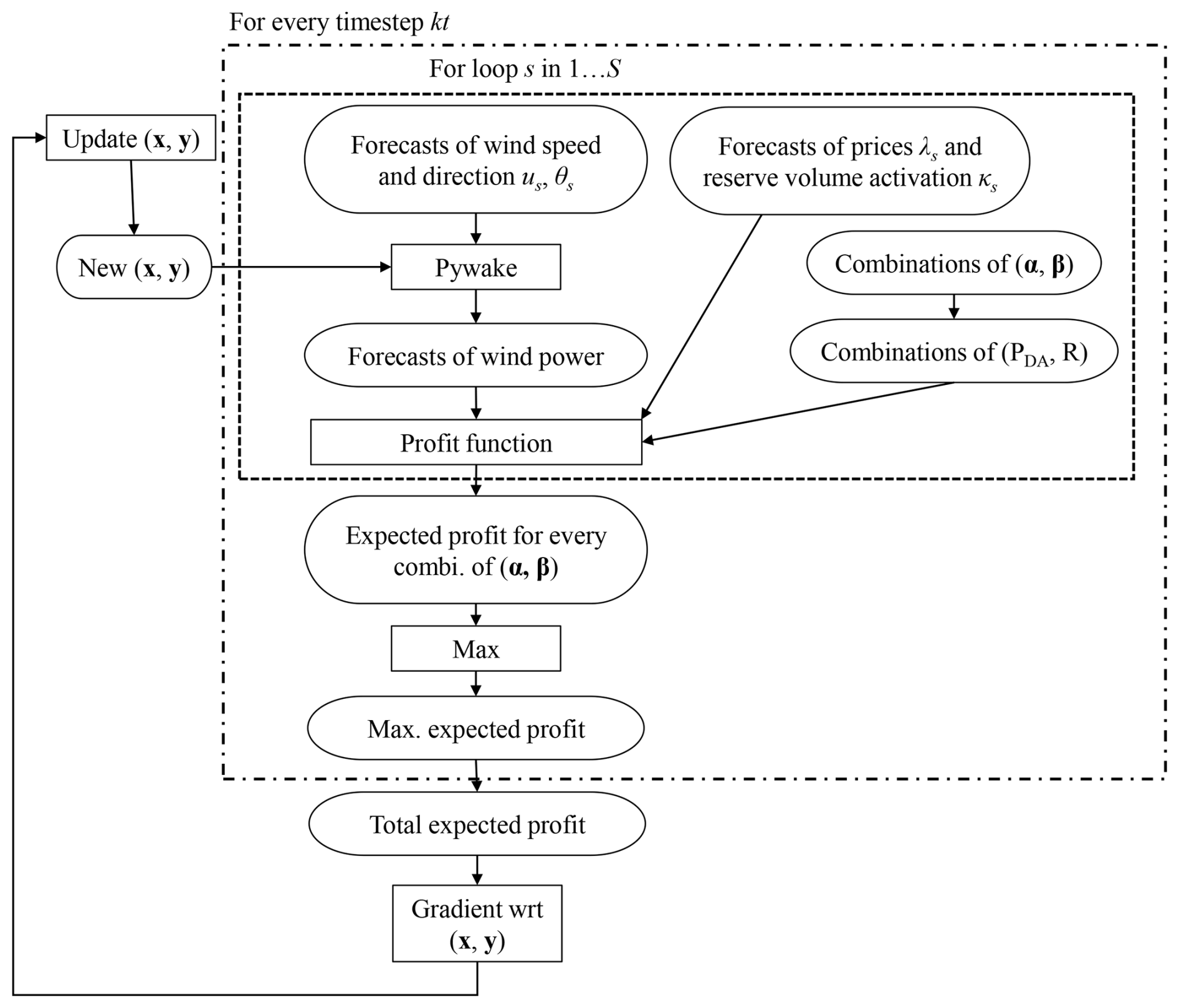
The optimization is carried out using stochastic gradient descent, which is an iterative method for optimizing a differentiable objective function. It replaces the actual gradient (calculated from the entire data set) by an estimate (calculated from a randomly selected subset of the data). Therefore, the algorithm follows the mean gradient by a specified distance, which is equivalent to optimizing the expected value of the objective function (Quick et al., 2023). This reduces the very high computational burden in high-dimensional optimization problems, achieving faster iterations but at the cost of a lower convergence rate. The inner optimization for the optimal bidding strategy in the JERM, defined by Eq. (11), is solved through a combinatorial exploration, which makes it differentiable and thus compatible with the SGD algorithm. Because computing the total revenue for a year (365 d ⋅ 96 quarters of an hour, i.e. 35 040 time steps) at each iteration would be too costly, SGD is particularly relevant for our proposed WFLO formulation.

3 Test case

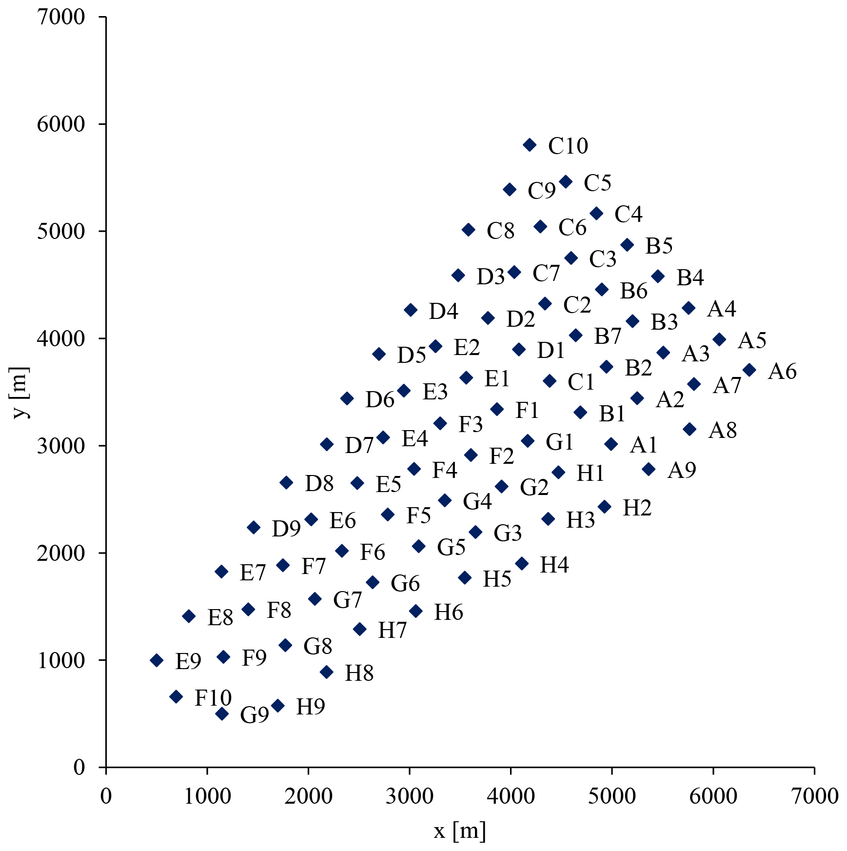
We use data from Northwind, a Belgian offshore wind farm situated 38 km from the coast, in the North Sea, within the first Belgian offshore cluster. Northwind consists of 72 Vestas turbines, for a total installed capacity of 216 MW. Each turbine has a rotor diameter of 112 m, a hub height of 71 m, and rated power of 3.075 MW. The layout of this wind farm can be seen in Fig. 3.

Figure 3 Layout of Northwind offshore wind farm.

Before optimizing the layout, expected yearly revenues and supplied energy are computed for the current built layout (further referred to as the base layout) for different modes of operation (with and without reserve). Then the maximum amount of power that can be allocated to reserve R_max is set to different values. First, Elia set a limit of 50 MW per delivery point in its current BSP agreement. Then, the required volume of aFRR reserves that Elia should ensure throughout the year was 117 MW for 2023 (total reserve capacity contracted by Elia at all times). This value is updated every year and is computed using a probabilistic method based on a time series of 2 years of expected variations between quarter-hours of system imbalances (ENTSO-E, 2024). However, with the growing penetration of renewable energies foreseen in the future, one can expect that this requirement will increase as well. Indeed, power systems will become highly weather-dependent and thus more prone to variability and unpredictability. We therefore set two more values for the maximum allocated reserve: Elia's total aFRR needs (approximately equal to half of the wind farm rated capacity if the operator wants to keep some available wind power for other markets) and the full farm capacity.

First, to compare with state-of-the-art WFLO formulations, the layout will be optimized with the objective of maximizing AEP. To assess the influence of accounting for electricity prices in the WFLO process, optimization with the day-ahead market only is also simulated. Finally, WFLO is carried out with the new formulation for the objective function that maximizes revenue from both day-ahead and reserve markets. Results will be compared with the two previous optimizations in terms of expected yearly revenues and yearly production. Historical data from 2023 in Belgium (see Sect. 3.1) are used during the optimization process. Moreover, it is important that the optimal layouts are relevant not only for the data used in the optimization process. Therefore, yearly revenues are also computed for unseen data, i.e. historical data from another year (2024). Those data were not seen during the layout optimization process but are nevertheless used to optimize bidding for that year.

The new objective function for WFLO has been integrated into the TOPFARM framework (Riva et al., 2024), comprising the SGD optimizer. Revenue and AEP gradients are computed using automatic differentiation. Turbine powers are obtained from Pywake simulations (Pedersen et al., 2023) using the Bastankhah Gaussian wake model for velocity deficits, the Crespo–Hernandez turbulence model for added turbulence, and linear superposition. The wind power modelling error for the forecast of power prediction is based on comparisons of PyWake with SCADA found in the literature (Van Binsbergen et al., 2024). The mean forecast error is set to 0 and the standard deviation to 3 %. The minimum turbine spacing d_min (constraint of Eq. 15) is set to 2 rotor diameters. The SGD optimizations are carried out using the following parameters: the initial learning rate is 1 rotor diameter, the maximum number of iterations is 2000, and the initial value for constraint aggregation multiplier is 0.1. We use several values of K⋅T (numbers of samples for every SGD iteration) when optimizing for revenues and AEP (K⋅T ranging from 20 to 150). To avoid unlucky sampling pitfalls, each case of SGD optimization is run using five different initial random starting conditions.

3.1 Analysis of historical data in Belgium

To help better understand the motivations of this work, we analyse historical data on wind, electricity prices, and activated reserve volume for the year 2023 in Belgium. Data on wind speed and wind direction at the location of the offshore wind farms in the Belgian North Sea have been gathered from the ERA5 database. Electricity prices for the day-ahead market were available on the European Network of Transmission System Operators (ENTSO-E) transparency platform (ENTSO-E, 2025). Prices for reserve capacity and reserve activation, as well as activated upward aFRR reserve volumes, were provided by Elia, the Belgian TSO (Elia, 2025). From Fig. 4, we can study the variations in price with regard to wind direction and wind speed and the mean activated reserve per wind sector. It can be seen in Fig. 4a that mean day-ahead prices do not follow the same pattern as mean reserve capacity and activation prices with regard to wind direction. Indeed, mean day-ahead prices show a lower mean value for the wind sector centred around 230°. This wind sector corresponds to the direction of dominant wind in this area of the North Sea (direction with most occurrences), as can be seen in Fig. 5. This leads to a discrepancy between maximizing revenues and energy production. Indeed, when prices are not considered, WFLO will try to avoid aligning turbines in the dominant wind direction. However, since prices tend to be lower in that wind section, it might be more profitable to avoid wake losses in other directions, where prices are higher. Mean reserve capacity prices, on the other hand, tend to be higher in that wind direction sector, while reserve activation prices do not show a significant increase or decrease. This means that accounting for participation in reserve will affect the optimization results, as day-ahead and reserve prices have different patterns with regard to wind direction. Figure 4c shows the volumes of activated reserve normalized by the maximum activated volume for aFRR upward reserve (117 MW in 2023). We can see that mean activated volumes tend to be lower in the direction of dominant wind. Another interesting analysis can be made in Fig. 4b, which displays the mean electricity prices with regard to wind speed. One can see that day-ahead prices tend to decrease with higher wind speeds, while it is the opposite for reserve capacity prices. One factor that explains this reduction of day-ahead price with increasing wind speed is the high penetration of offshore wind generation in the Belgian power system (10 % of yearly consumption produced by offshore wind farms). Because wind energy has lower production costs than conventional thermal power plants, a high production of electricity through wind turbines can lead to lower prices in the day-ahead market. Reserve activation prices remain constant until approximately 20 m s⁻¹ but show a sharp increase around 25 m s⁻¹, which is the cut-off wind speed of most Belgian offshore wind turbines. This is the limit at which turbines are shut down to prevent mechanical damage, and the farm output goes from the rated power to 0. Therefore, a small prediction error in wind speed can lead to a tremendous need for reserve.

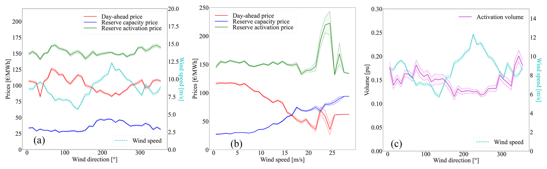
Figure 4 Mean electricity prices with regard to (a) wind direction and (b) wind speed in 2023. (c) Mean normalized activated volumes of reserve with regard to wind direction.

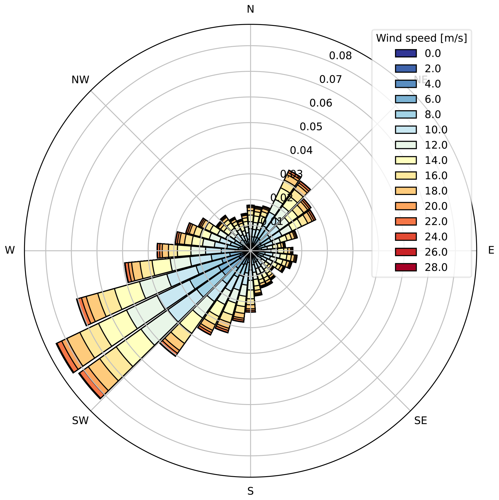
Figure 5 Wind rose at the location of Belgian offshore wind farms for 2023 from ERA5 data (latitude: 51.5° N, longitude: 2.75° E).

4 Results and discussion

4.1 Operating the current built layout with reserve participation

Before optimizing the layout of the Northwind wind farm, yearly revenues are computed for the base layout (currently built) using historical data from 2023. Three modes of operation are considered:

• Produce as much wind power as possible (referred to as prod. max. operation in result tables). Energy bids are not risk-based as they only rely on forecasts of available power, regardless of market conditions. This is the most simple operation as the operator does not need to derate the turbines in the case of unfavourable market conjuncture.

• Wind power is only sold on the day-ahead market but energy bids are made based on forecasts of available wind power, day-ahead prices, and imbalance penalties (referred to as DAEM-optimized operation in result tables).

• Wind power is sold on JERM (provision of reserve).

The optimal allocation of day-ahead and reserve power on JERM is solved with Eq. (11) for every quarter of an hour of the year, and the expected revenues are summed over 35 040 time steps. The maximum value allowed for reserve bids is first set to 50 MW. The optimized operation on DAEM only uses the same formulation but with $R_{k,t}=\mathrm{0}\forall k,\forall t$. This allows assessing the impact of participating in the upward secondary reserve market.

The expected supplied energy is the yearly production of the farm actually injected to the grid. For the JERM case, it encompasses both the energy sold on the day-ahead energy market and the activated reserve. It should be noted that electrical losses and downtime due to maintenance and failures are not taken into account. AEP_theory is the theoretical yearly production of the farm, computed solely by converting data on wind speed and wind direction to potential wind power. It does not include any forecasting errors. Expected yearly revenues and supplied energy are reported as $\mathit{\mu }\pm \frac{\mathit{\sigma }}{\sqrt{S}}$, where the standard deviation relates to forecast uncertainty (sampling of S forecast errors).

It can be seen in Table 1 that operating Northwind for maximizing production leads to the lowest revenues. Indeed, making energy bids on DAEM only for revenue maximization increases expected yearly revenues by 6.51 %. This can be explained by two factors. First, producing too much wind power when day-ahead prices are negative is detrimental, but time steps with such prices only occur 2.52 % of the time in data from 2023. Then, forecasting prices allows adopting a risk-aware approach, i.e. bidding more when imbalance penalty prices are expected to be close to day-ahead prices (the risk is acceptable) and bidding less than the forecasted available power in the case of very high imbalance prices. This is confirmed in Table 2, which shows the revenue breakdown between positive revenues and imbalance penalties. Total imbalance penalties are higher when operating for revenue maximization, but the significant increase in positive revenues allows compensating for the penalties. Regarding supplied energy, maximizing production obviously leads to more wind power injected to the grid. The reduction of supplied energy of 4.47 % when maximizing DAEM revenues is very interesting because it could lead to lower load constraints on wind turbines, thus extending their lifetime. However, this aspect needs to be further investigated.

Table 1 Expected yearly revenues and supplied energy in 2023 for the initial base layout of Northwind, operated for maximizing production on DAEM (a, f), maximizing revenues on DAEM only (b, g), and maximizing revenues on JERM (c–e, h–j, with different values for maximum reserve bids R_max). Results are reported as $\mathit{\mu }\pm \frac{\mathit{\sigma }}{\sqrt{S}}$, where μ and σ relate to forecast uncertainty.

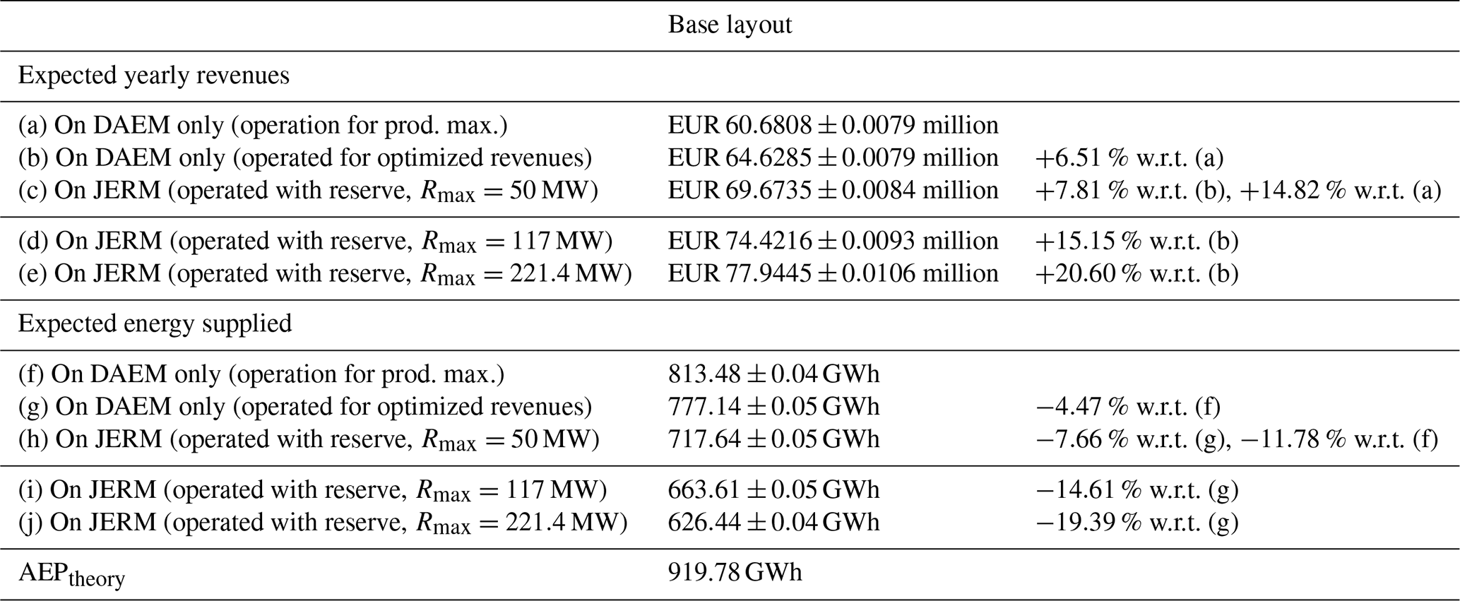
Table 2 Breakdown of expected yearly revenues in 2023 for the initial base layout of Northwind, operated for maximizing production on DAEM (a), maximizing revenues on DAEM only (b), and maximizing revenues on JERM (c, with maximum reserve bids R_max=50 MW).

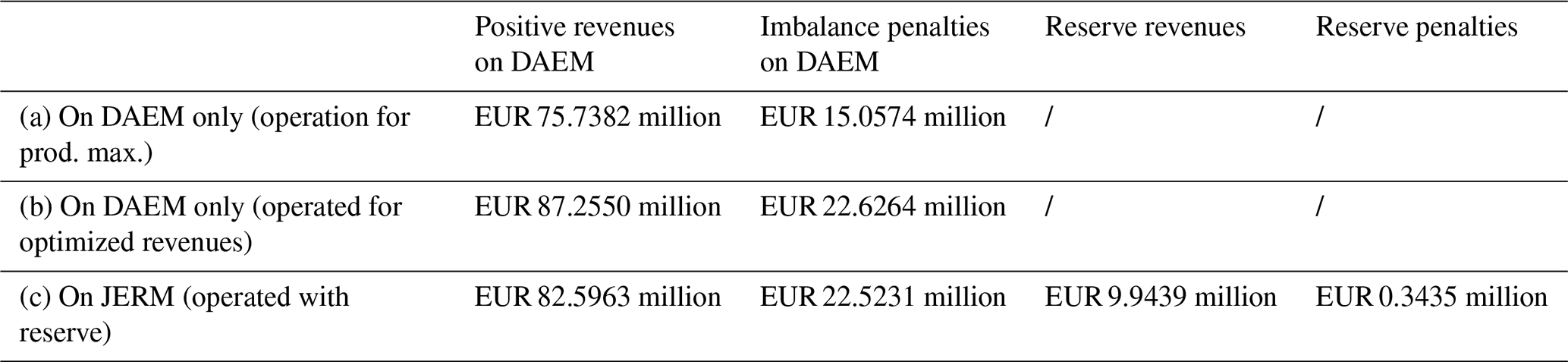
Supplying secondary upward reserve (operate the wind farm on JERM) increases expected yearly revenues by 7.81 %, while the supplied energy is decreased by 7.66 %. Indeed, bidding a given amount of power in the reserve capacity and energy markets does not mean that this power will be entirely supplied. If the system negative imbalance is not too severe, only a fraction of contracted reserves is actually activated by the TSO. However, the wind farm operator still earns revenues by making this power available to restore balance in the system. This is particularly profitable when day-ahead prices are very low. It can be seen in Table 2 that while positive revenues on DAEM are quite low when providing reserve (earnings are “transferred” to the reserve markets), imbalance penalties do not decrease significantly. This is inherent to our formulation because in the case of imbalance (the available wind power is lower than the total power bid on both DAEM and reserve markets), priority is given to the reserve provision.

Sensitivity to the reserve limit R_max

Currently, the maximum value per delivery point of reserve capacity bids established by Elia is 50 MW. Moreover, the static volume need of aFRR reserves for the Belgian power system in 2023 was set at 117 MW. However, as stated before, in future weather-dominated power systems, the need for frequency regulation, including aFRR, will increase. Therefore, the wind farm is operated considering for two other values of R_max: 117 MW (approximately $\mathrm{1}/\mathrm{2}$ of rated capacity in the case that the operator always wants to keep some available wind power for other markets) and 221.4 MW (full farm capacity).

With R_max=117 MW, it can be observed in Table 1 that for the base layout, expected yearly revenues increase by 15.15 % when the wind farm offers aFRR services, while supplied energy drops by 14.6 %. Compared to the previous case (R_max=50 MW), doubling the allowed maximum value for reserve capacity bids leads to a revenue improvement also multiplied by 2 (15.15 % against 7.81 % previously). Regarding yearly supplied energy (on DAEM and activated reserve), it decreases when R_max is increased (≈664 GWh against ≈718 GWh with R_max=50 MW). Indeed, allowing for higher reserve bids enables wind farms to participate more in frequency reserve services. But if reserve energy bids are not entirely activated by the TSO, less energy is supplied, while revenues are increased.

With the full wind farm capacity (221.4 MW) as R_max, expected yearly revenues on JERM in 2023 for the base layout are even higher. However, even though R_max is doubled compared to the previous case, revenue increments are not multiplied by 2 this time. Indeed, the improvement is at 20.60 % against 15.15 % when R_max was set at 117 MW. This shows a flattening of revenue augmentation, and wind farm operators might want to avoid allocating all available power to the reserve market. Indeed, because of potential forecast errors, there is a significant risk of bidding in only one market, and operators could want to keep some available wind power for other markets (or even a security margin to avoid penalties when the contracted power cannot be entirely supplied).

4.2 Optimized layout for AEP maximization

We first optimize the layout with the objective function widely used in the current literature, i.e. AEP maximization. For the latter, wind speeds and wind directions from the 2023 historical data are used during the optimization process. SGD optimizations are performed for different values of Monte Carlo samples (K⋅T) and several initial conditions. Reported results are those obtained with the best optimized layout out of all simulations, i.e. the one leading to the highest AEP. Again, expected revenues and energy supplied are computed for the three modes of operation (maximizing production, maximizing expected revenues on DAEM only, and maximizing expected revenues on JERM). Moreover, it is worth reminding the reader that while the total energy supplied indicates the actual electricity sold (or activated in the case of reserve provision) and injected to the grid, AEP gives the theoretical energy that could be supplied by the wind farm given the wind conditions, regardless of prices and errors in wind power forecasts.

Table 3 Expected yearly revenues and supplied energy in 2023 for the base layout and the best layout optimized for AEP, operated for maximizing production on DAEM (a, d), maximizing revenues on DAEM only (b, e), and maximizing revenues on JERM (c, f, with maximum reserve bids R_max=50 MW). Results are reported as $\mathit{\mu }\pm \frac{\mathit{\sigma }}{\sqrt{S}}$, where μ and σ relate to forecast uncertainty.

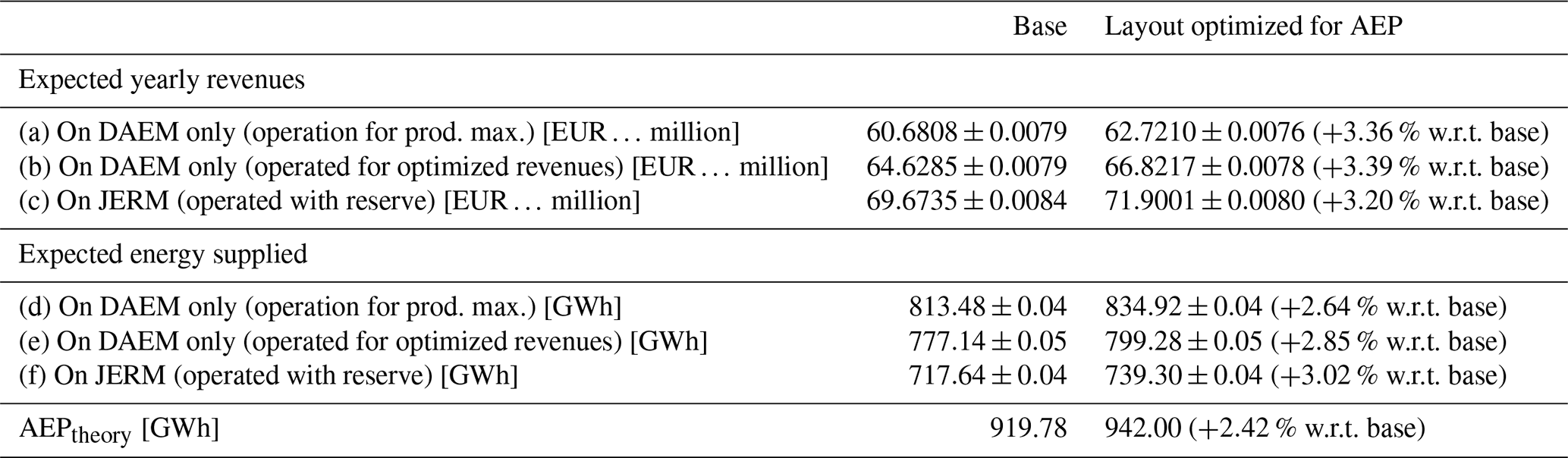
As can be seen in Table 3, the best optimized layout for AEP leads to an increase in yearly revenues on JERM by 3.20 %, as well as 3.02 % more supplied energy. Indeed, a better placement of wind turbines avoids wake losses and leads to improved electricity production in general. Considering that the average lifespan of an offshore wind farm is approximately 20 years (Topham and McMillan, 2017), a revenue increased by EUR 2.23 million yr⁻¹ leads to a significant improvement in the wind farm profitability: more than EUR 44 million over the farm lifetime. Therefore, an improvement in expected revenues on both DAEM and JERM is firstly obtained through an improvement in AEP.

4.3 Optimized layout for revenue maximization on day-ahead market only

To assess the impact of including market conditions (e.g. electricity prices) in the layout optimization process, the objective function has been modified to maximize expected revenues from the day-ahead market only (i.e. setting R_max=0 MW in Eq. 13). This is later referred to as the DAEM-optimized case. Like before, SGD optimizations are performed for different values of Monte Carlo samples (K⋅T) and several initial conditions. Reported results are those obtained with the best optimized layout out of all simulations, i.e. the one leading to the highest expected revenues on DAEM.

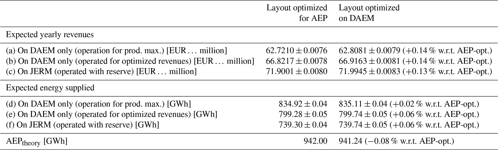
As can be seen in Table 4, the best layout optimized to maximize expected revenues on DAEM leads to an increase in yearly revenues on JERM by 0.13 % compared to the best optimized layout for AEP, and the theoretical AEP moderately decreases. The explanation for this slight increase in expected revenues is that the objective function for AEP aims at maximizing the power output of a wind farm regardless of electricity prices. It usually avoids wake losses for the directions of dominant wind. However, if low or even negative prices are associated with those directions, then revenues will not increase. Moreover, besides revenues, it is not beneficial for the grid that wind farms produce a lot of electricity when prices are quite low. Indeed, for power systems with a high penetration of renewable energies, especially wind, low or even negative prices may correspond to periods of overproduction; i.e. generation exceeds consumption. In that case, wind turbines might have to be shut down to curtail wind energy and restore balance in the system. This spillage of renewable energy is of course not desirable, and it is much more relevant to optimize wind farm layouts so that they produce more energy during times of low generation in the system (usually associated with higher prices). This also explains why expected revenues increase despite a slight reduction in AEP. Therefore, an improvement in expected revenues on both DAEM and JERM is secondly obtained through inclusion of electricity prices in the optimization process.

Table 4 Expected yearly revenues and supplied energy in 2023 for the best layout optimized on DAEM, operated for maximizing production on DAEM (a, d), maximizing revenues on DAEM only (b, e), and maximizing revenues on JERM (c, f, with maximum reserve bids R_max=50 MW). Results are reported as $\mathit{\mu }\pm \frac{\mathit{\sigma }}{\sqrt{S}}$, where μ and σ relate to forecast uncertainty.

4.4 Optimized layout accounting for reserve participation

WFLO is carried out with the objective of maximizing revenues on JERM, i.e. accounting for participation in reserve markets. SGD optimizations are performed for different values of Monte Carlo samples (K⋅T) and several initial conditions. Reported results are those obtained with the best optimized layout out of all simulations, i.e. the one leading to the highest expected yearly revenues on JERM. To assess the impact of including reserve provision in the layout optimization process, the results are compared with the best layout optimized on DAEM, obtained in the previous section.

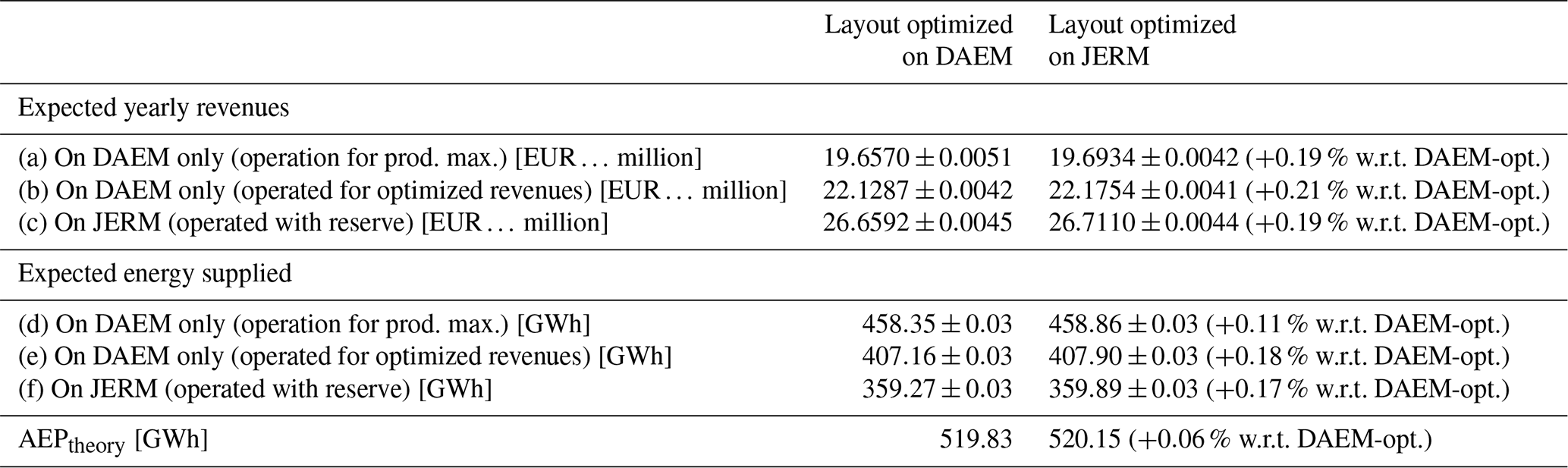
As can be seen in Table 5, the best layout optimized to maximize expected revenues on JERM leads to an increase in yearly revenues on JERM by 0.13 % compared to the best optimized layout on DAEM. We also observe a moderate increase in expected energy supplied and AEP. The slight augmentation in expected revenues could be explained by two factors. On the one hand, better placement of wind turbines to avoid wake losses leads to an improved AEP and electricity production in general. On the other hand, the inclusion of reserves in the objective function better reflects real-world market conditions and ensures that layouts are evaluated under more comprehensive profitability criteria (and not just energy yield). Even though revenue differences could be considered small (∼0.1 %–0.2 %), they are economically meaningful at scale. It should be noted that these numbers cannot be directly generalized for other electricity pools, but since most European electricity markets have a similar structure, applying this methodology is also expected to result in higher yearly revenues for layouts optimized for revenue maximization with reserve participation. Therefore, a slight improvement in expected revenues on both DAEM and JERM is thirdly obtained through inclusion of more comprehensive market conditions, i.e. provision of reserve, in the optimization process.

Table 5 Expected yearly revenues and supplied energy in 2023 for the best layout optimized on JERM, operated for maximizing production on DAEM (a, d), maximizing revenues on DAEM only (b, e), and maximizing revenues on JERM (c, f, with maximum reserve bids R_max=50 MW). Results are reported as $\mathit{\mu }\pm \frac{\mathit{\sigma }}{\sqrt{S}}$, where μ and σ relate to forecast uncertainty.

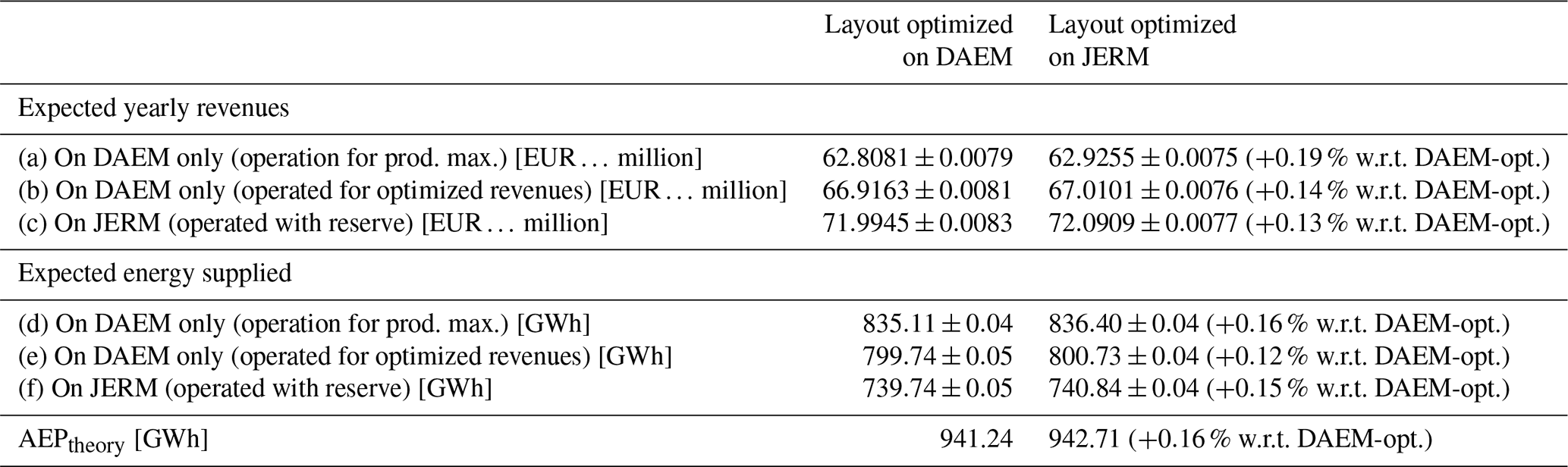
Surprisingly, the best total yearly revenues on DAEM only are obtained for the best layout optimized with reserve. One reason for this is that during the optimization without reserve, the wind farm can only participate in one market (the DAEM). If day-ahead prices are very low or negative, the wind farm will not bid on the DAEM, resulting in no revenue, thus leading to a zero gradient and the solution space being less explored. This means that even if reserve market rules change dramatically, causing the wind farm to be unable to participate in the reserve market, operating the optimized layout with reserve on DAEM only would still be profitable.

For every obtained layout optimized on DAEM (no reserve) and on JERM (reserve participation in the objective function), expected revenues on DAEM only (i.e. wind farm operated without reserve) and on JERM are computed.

Figure 6 shows the expected yearly revenues on JERM as a function of expected yearly revenues on DAEM only for the layouts optimized for revenue maximization with and without reserve participation. The scatter points show that, over several runs of the training algorithm, the maximum profits can be gained by the JERM-optimized layout, and the outcomes also reveal that these optimized layouts for JERM are better on average. The whole distribution of profits (over experiments) is improved, not only extreme points. While the stochastic nature of the layout optimization introduces variability in the results, JERM-optimized layouts are at least as effective as DAEM-optimized layouts and even offer slight improvements.

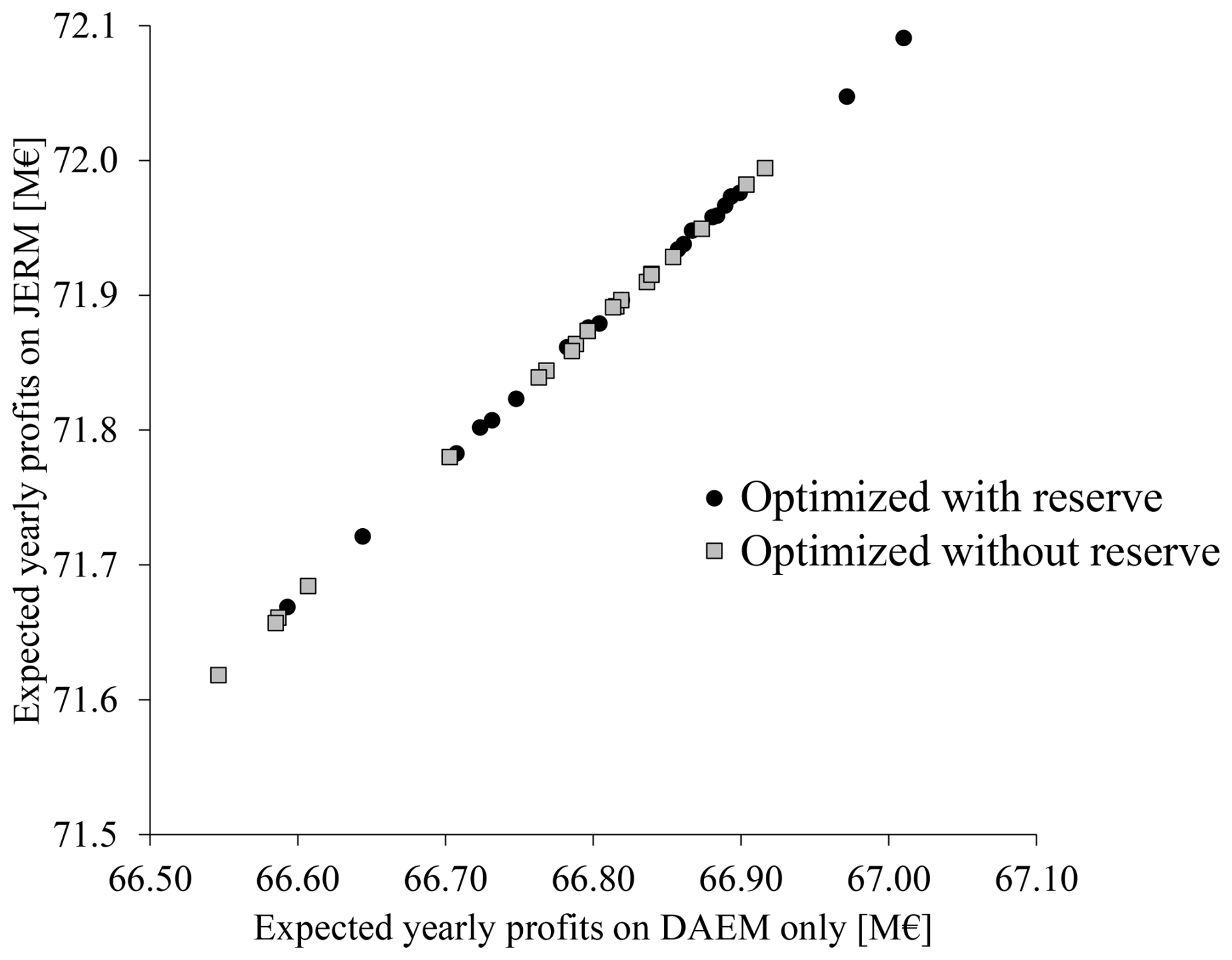
Figure 6 Expected yearly revenues on JERM plotted versus expected yearly revenues on DAEM only (wind farm operated without reserve). Each point corresponds to one optimized layout, with the black circles representing layouts optimized with reserve, and the grey squares are for layouts optimized without reserve.

The best optimized layout on JERM is plotted in Fig. 7 and compared to the current layout of Northwind. Turbines that were on the farm boundaries in the base layout kept their position on the outer limits (even though turbines had random positions in the starting initial conditions of the optimization). However, inner turbine positions have been significantly modified compared to the base layout. Indeed, while the structure of rows has been approximately maintained, it can be observed that more turbines are placed together in a row, while consecutive rows are more distant from one another and are not parallel (which was the case for all rows in the base layout). A few turbines have a more irregular position (in between rows).

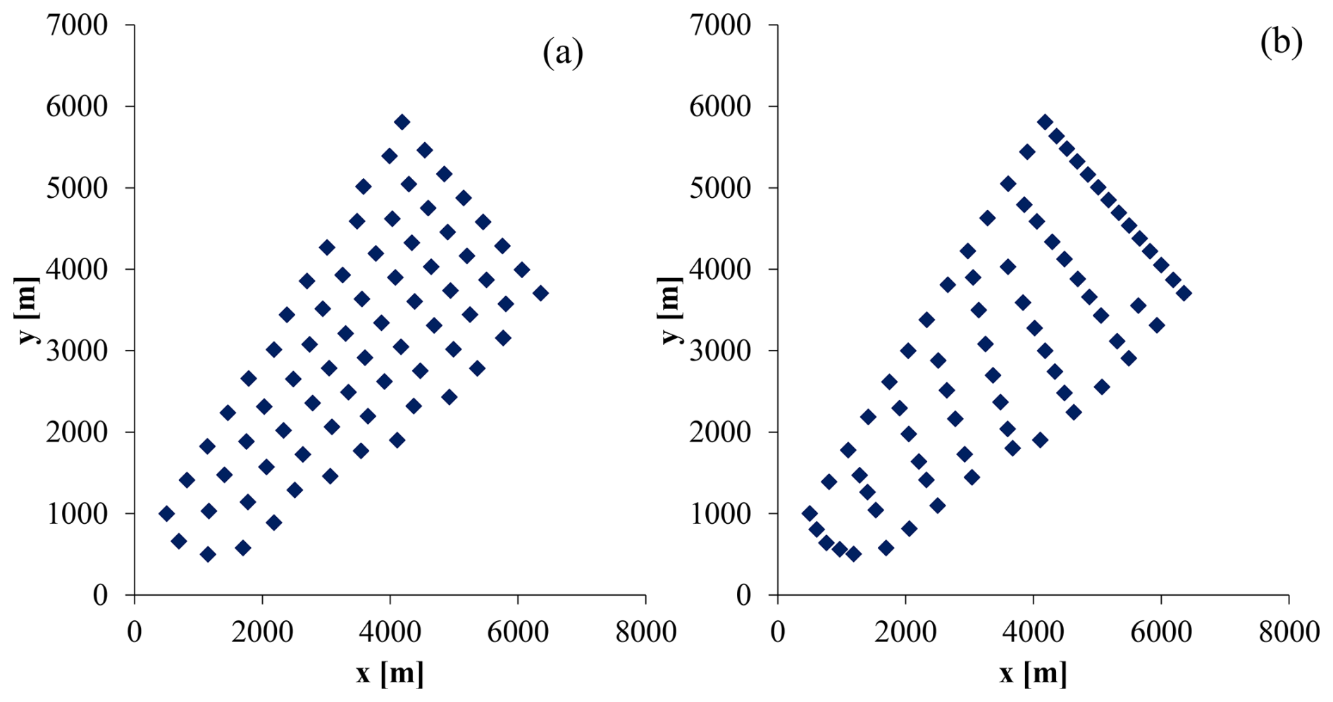
Figure 7 (a) Base layout of Northwind offshore wind farm. (b) Best layout optimized for revenue maximization with participation in the reserve market.

Another interesting characteristic to compare between the optimized and base layouts is the power rose. It shows the power output of the wind farm with regard to wind direction for a given wind speed. In Fig. 8, the power is normalized by the wind farm rated capacity (for Northwind, 221.4 MW). It allows identifying the wind directions leading to higher wake losses.

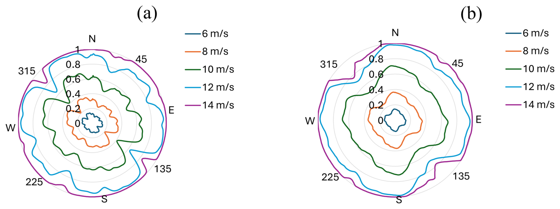
Figure 8 Power roses of Northwind (a) base layout. (b) Layout optimized for revenue maximization in JERM.

The power rose in Fig. 8a shows that the base layout exhibits many power drops, with wake losses being the most severe for directions of 135 and 315° (0° corresponds to wind blowing from the north, then clockwise counting). This pattern is inherent to regular layouts, where turbines are placed in rows equidistant from each other and wake losses are at their maximum when most turbines are aligned with the wind direction. In Fig. 8b, wake losses are still prevalent for wind directions of 135 and 315°, but they are less severe, and power drops are smoothed for other directions. Indeed, while still located in rows, turbines from different rows are more distant, allowing wind speed to recover between consecutive rows. However, it should be noted that a more irregular turbine placement can lead to higher installation costs and fatigue loading (Sickler et al., 2023).

4.4.1 Comparison with optimized layout for AEP maximization

We also compare our novel formulation for WFLO with the objective function widely used in the current literature, i.e. AEP maximization. The yearly expected revenues and AEP results are summarized in the box plots in Fig. 9, where optimizations were run for different values of K⋅T and five different initial random conditions for each. We can see that yearly expected revenues are higher for layouts optimized with our new objective function. The mean yearly expected revenue for JERM optimizations is EUR 71.8956 ± 0.105 million, while it is EUR 71.7638 ± 0.106 million for AEP optimizations. The mean absolute difference is EUR 0.1318 million, i.e. 0.18 %, thus with increased revenues of EUR 2.6 million over the farm lifetime. However, for AEP, no strong claim can be made regarding the superiority of one of the optimizations. Indeed, the difference in AEP, approximately equal to 0.05 %, is lower than the uncertainties in energy metrics.

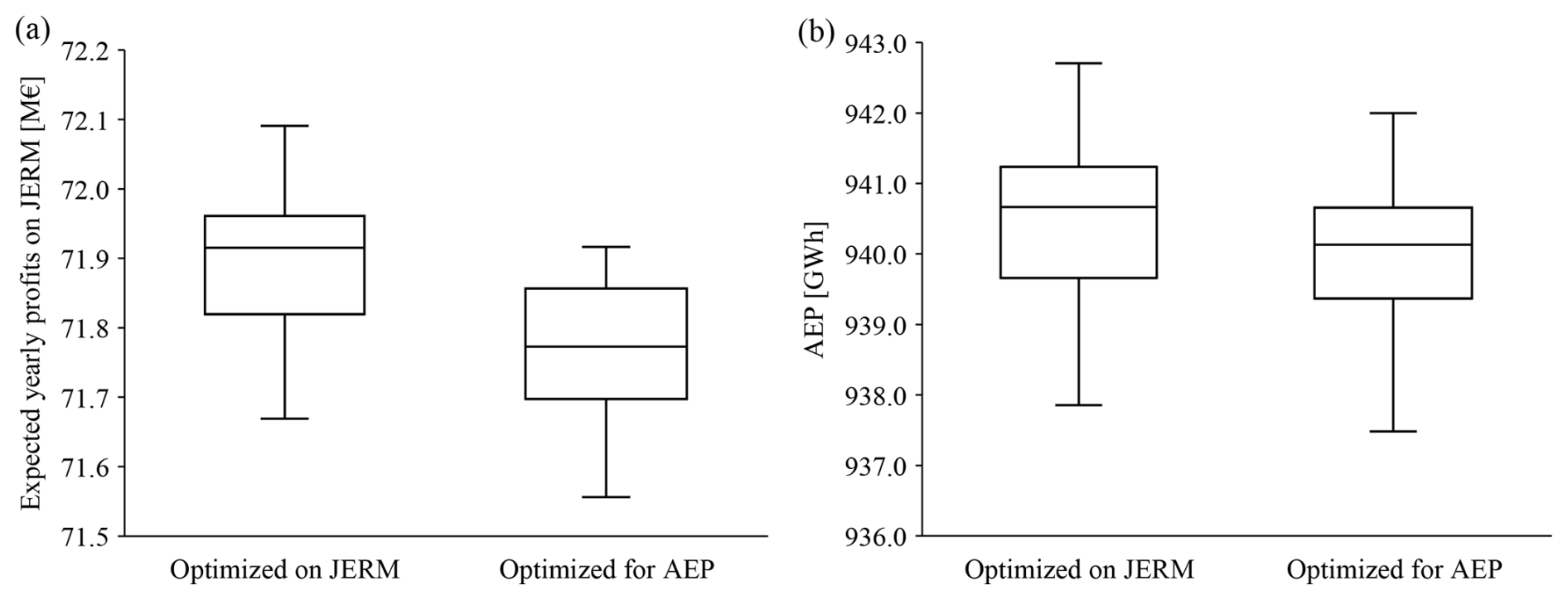
Figure 9 Optimization results associated with AEP optimizations and JERM optimizations. The yearly expected revenues (a) and AEP (b) are plotted as box and whisker plots.

Figure 10 shows the expected yearly revenues on JERM as a function of AEP for the layouts optimized for revenue maximization with reserve and AEP maximization. The uppermost black circle on the right represents the optimized layout giving the highest revenues on JERM but also the highest AEP. It should be noted that this layout corresponds to the best layout optimized for revenue maximization with reserve, for which results are given in Table 5. It is quite surprising that the best AEP is not obtained for a layout optimized for AEP maximization. This aspect should be further investigated in future work.

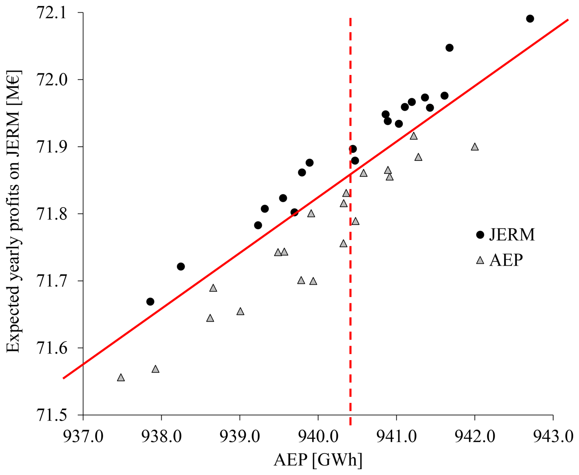
Figure 10 Expected yearly revenues on JERM plotted versus AEP. Each point corresponds to one optimized layout, with the black circles representing layouts optimized with reserve, and the grey triangles are for layouts optimized for AEP maximization.

Another interesting observation is that yearly revenues on JERM are generally higher for layouts optimized for revenue maximization with reserve: if a diagonal is drawn in the scatterplot, all triangles are located below that line compared to the circles. And if a vertical line is plotted for a given AEP, black circles are always located above the triangles. In other words, for the same level of AEP, the layouts optimized for reserve lead to higher revenues on JERM than the ones obtained for AEP maximization.

4.5 Generalization to unseen future data

In Sect. 4.2–4.4, historical data from 2023 were used during the SGD optimizations, as well as for the computation of expected yearly revenues for the optimized layouts. In this section, revenues and supplied energy will be assessed with historical data from 2024, i.e. data unseen during the optimization process. Indeed, it is valuable to have optimized layouts that also yield improved revenues for future years.

First, wind data and electricity prices from January to July 2024 are analysed. The wind rose of 2024, plotted in Fig. 12, shows patterns comparable with 2023: dominant wind directions are mostly south-westerly. More wind blowing from the north-east is visible in Fig. 5, which is not the case here. It can be seen in Fig. 11a that day-ahead prices, similar to 2023, have lower values for the direction of dominant winds, although this is less noticeable than in 2023. Moreover, day-ahead prices in 2024 have overall lower mean values than in 2023. Reserve capacity prices do not vary much with wind direction, while activation prices show more variability but no significant drop for the directions of dominant wind. The overall mean values are of the same order of magnitude as for the previous year, and we again observe a sharp increase in reserve activation prices between 20 and 25 m s⁻¹. However, this peak is less pronounced, with a mean peak value under 200 EUR MWh⁻¹, while it reached almost 250 EUR MWh⁻¹ in 2023. This could be explained by fewer sudden-high-wind events (e.g. storms), a smoother farm cut-out, or better anticipation by the TSO. Normalized activation volumes exhibit lower values for directions of dominant wind. Therefore, while the wind, prices, and activated reserve volume of 2024 share some similarities with data from 2023, they also exhibit noticeable differences. They are thus relevant to test the validity of the optimized layouts on unseen data. The case presented here uses R_max=50 MW when the wind farm is operated with reserve.

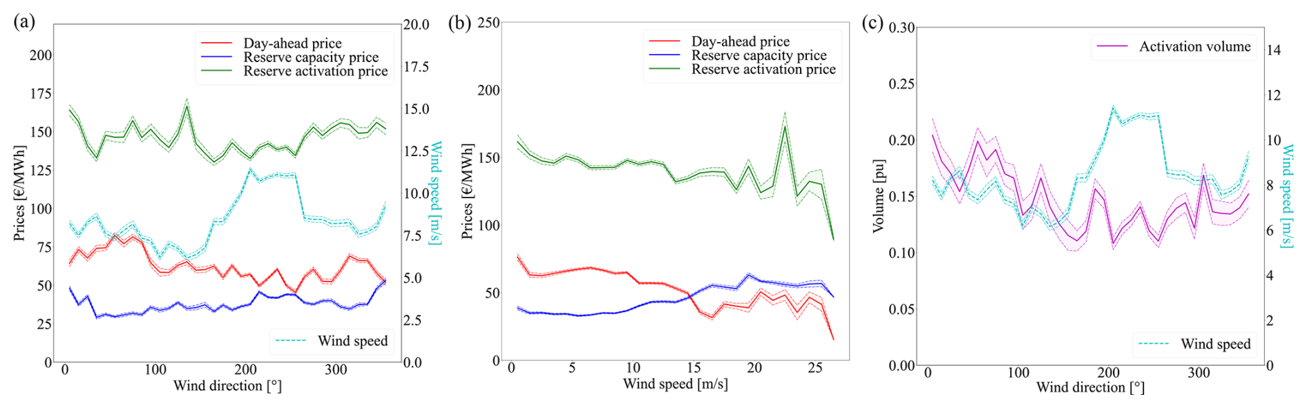
Figure 11 Mean electricity prices with regard to (a) wind direction and (b) wind speed in 2024. (c) Mean normalized activated volumes of reserve with regard to wind direction.

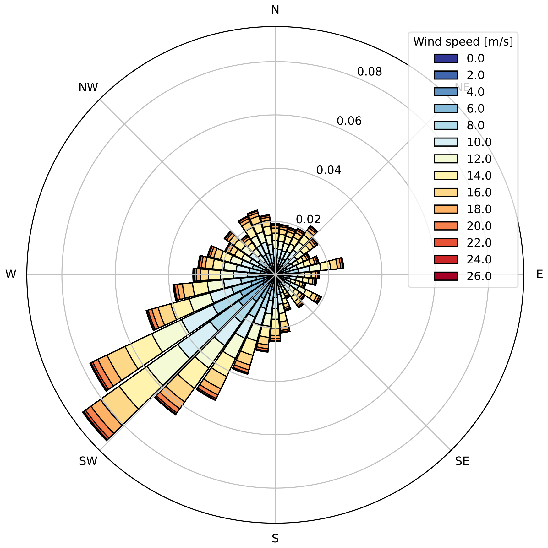
Figure 12 Wind rose at the location of Belgian offshore wind farms for 2024 from ERA5 data (latitude: 51.5° N, longitude: 2.75° E).

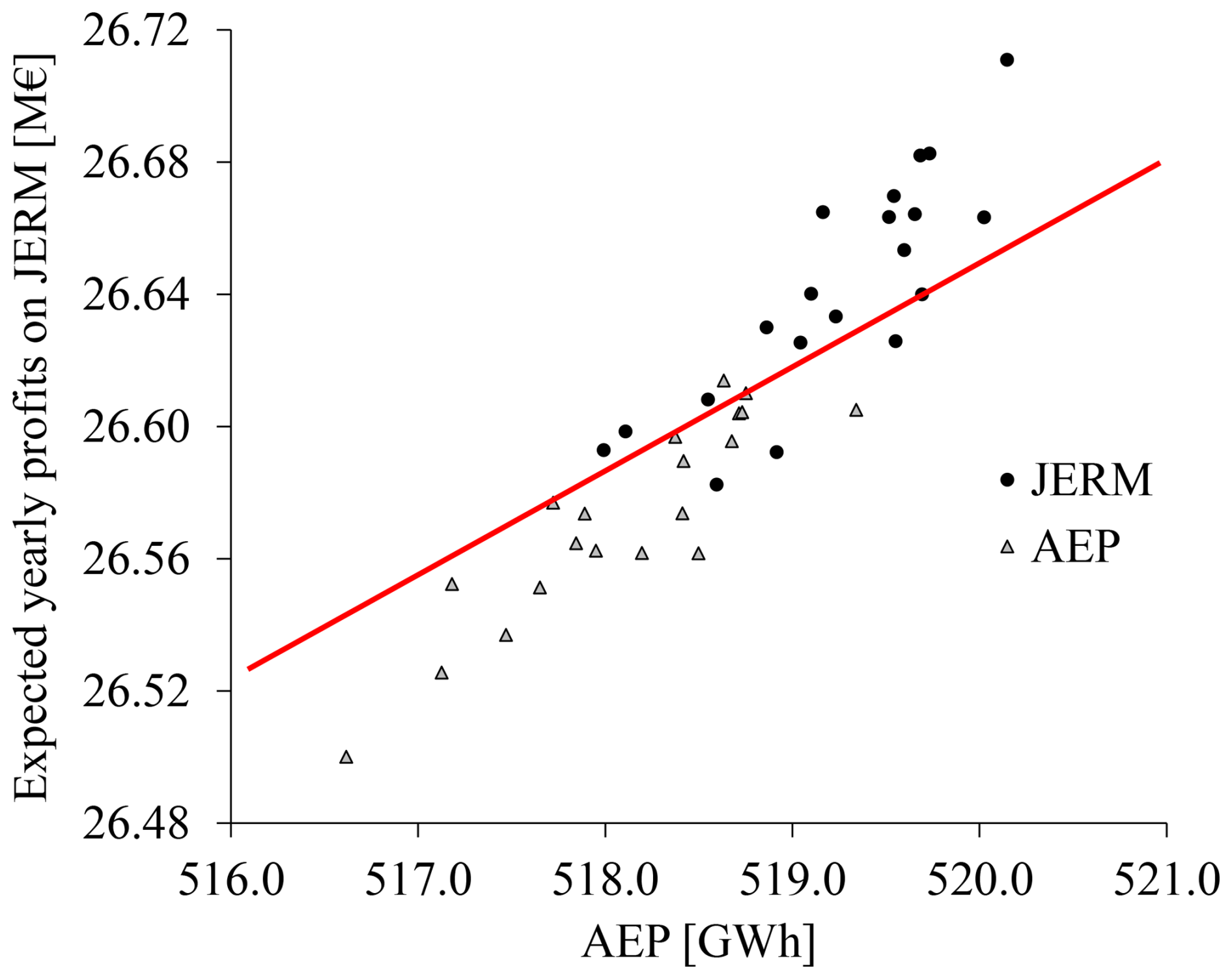
Figure 13 Expected yearly revenues on JERM in 2024 plotted versus AEP. Each point corresponds to one layout optimized using 2023 data, with the black circles representing layouts optimized with reserve, and the grey triangles are for layouts optimized for AEP maximization.

For the base layout, it can be observed in Table 6 that results show the same trends already noticed for 2023: revenues on DAEM only are increased when energy bids are made to maximize revenues and not power production. Participating in reserve leads to yearly revenues improved by 20.96 %, while it was only 7.82 % for 2023. A reason for this better improvement is the overall lower values of day-ahead prices in 2024, thus giving more opportunities to make revenues on reserve markets. Indeed, allowing participation in reserve markets increases revenues significantly when the day-ahead market is less profitable.

The best layout optimized for AEP is the same as the one presented in Table 3, i.e. optimized with 2023 data. When operated using 2024 data, the optimized layout leads to higher total revenues and supplied energy, of the same order of magnitude as for 2023. These results show that the optimized layout obtained with data from 2023 is still relevant for 2024, even though both years showed dissimilarities in wind distribution. Therefore, the best optimized layout for AEP shows robustness to wind conditions.

In Table 7, the best layouts are the same as the ones presented in Table 5, i.e. optimized with 2023 data. When operated using 2024 data, the optimized layout on JERM leads to slightly higher total revenues and supplied energy. These results show that the JERM-optimized layout obtained with data from 2023 is still relevant for 2024, even though both years have dissimilarities in wind distribution and prices. Therefore, the best optimized layout on JERM shows robustness to market conditions.

Table 6 Expected yearly revenues and supplied energy in 2024 for the base and best layout optimized for AEP with 2023 data, both operated for maximizing production on DAEM (a, d), maximizing revenues on DAEM only (b, e), and maximizing revenues on JERM (c, f, with maximum reserve bids R_max=50 MW). Results are reported as $\mathit{\mu }\pm \frac{\mathit{\sigma }}{\sqrt{S}}$, where μ and σ relate to forecast uncertainty.

Table 7 Expected yearly revenues and supplied energy in 2024 for the base and best layout optimized for DAEM and JERM with 2023 data, both operated for maximizing production on DAEM (a, d), maximizing revenues on DAEM only (b, e), and maximizing revenues on JERM (c, f, with maximum reserve bids R_max=50 MW). Results are reported as $\mathit{\mu }\pm \frac{\mathit{\sigma }}{\sqrt{S}}$, where μ and σ relate to forecast uncertainty.

Finally, if we again compare our methodology with the AEP maximization formulation, we observe the same patterns as for 2023. Indeed, when plotting expected yearly revenues on JERM as a function of AEP, for layouts optimized for revenues on JERM and for AEP, we still see in Fig. 13 that the grey triangles representing layouts for AEP maximization are generally below the black circles.

5 Conclusions

In the coming years, offshore wind farms are expected to have a significant role in restoring frequency balance through the provision of reserve. If reserve markets grow and the contribution of wind farms to reserve provision becomes important, then future farms should account for those flexibility requirements in their design procedure, even though the limited size of the reserve market might not allow every wind farm to fully participate. In this paper, a new methodology for WFLO is developed to account for future offshore wind farms participating in secondary upward reserve markets. The objective function aims at maximizing revenues from both day-ahead and reserve markets. It uses stochastic gradient descent for the optimization and probabilistic forecasts of wind power and electricity prices. An inner optimization problem provides the total power contracted on the JERM and the allocation of power to reserve procurement purposes.

When applied to a real-life Belgian test case, results show that yearly revenues are expected to increase in a significant way when accounting for participation in reserve markets, while exhibiting a lower supplied energy. This revenue augmentation is amplified when the maximum value for reserve bids is larger. The layout was then optimized for different objectives. A first increase in expected revenues and AEP is obtained by optimizing the layout for AEP, i.e. the objective function widely used in the literature. Another increase was observed when maximizing expected revenues on the day-ahead market instead of AEP. Indeed, this allows including electricity prices in the optimization process. Thirdly, a slight augmentation is seen when including participation in reserve markets in the objective function. Indeed, this allows better reflecting real-world market conditions and ensures that layouts are evaluated under more comprehensive profitability criteria. Although revenue differences are small (∼0.1 %–0.3 %), JERM-optimized layouts consistently perform at least as well as, and occasionally better than, DAEM-optimized ones. Finally, the optimized layouts also yield better revenues when computed using unseen data. Besides higher revenues, it is critical that wind farms are designed to produce more energy when prices are higher, usually corresponding to periods of low electricity production. Maximizing production when prices are low or even negative, generally associated with a surplus of generation, leads to spillage of renewable energy.

The perspectives of this work are twofold. First, a better modelling of forecast errors could take into account cross-correlation between wind, price, and activated reserve forecasts (though this would not change the WFLO formulation). Secondly, the impact on blade loads could be relevant to assess the costs versus benefits of providing reserve services. Indeed, wind farms participating in the reserve market should have less fatigue loading due to a reduced activity (less energy supplied), which would increase the farm lifetime and reduce the operation and maintenance costs of the wind farm components.