Near-wake behavior of an asymmetric wind turbine rotor

With symmetric rotors, tip vortex helices develop regularly before experiencing the leapfrogging instability. This instability can occur earlier when the consecutive helices are radially offset, which is the case for a rotor with non-identical blade lengths. Inspired by this, the current study investigates the spatiotemporal development of near-wake behavior for a rotor with significant blade length differences. Large-eddy simulations with an actuator line model are performed on a two-bladed wind turbine rotor under laminar and turbulent inflow conditions to evaluate the impacts of blade length differences ranging from 0 % to 30 % of its radius. The study analyzes the formation and development of helical tip vortices, the onset of leapfrogging, and the growth rate of this instability. The results show that the relative distance where leapfrogging takes place and the growth rate of the leapfrogging instability both decrease with increasing blade length difference, which agrees fairly well with the prediction of the two-dimensional point vortex model. The results also reveal that the effects of inflow turbulence on the leapfrogging instability are minimal in the context of the growth rate. While the considered rotor asymmetries accelerate the leapfrogging, the outcomes demonstrate that the leapfrogging does not necessarily induce large-scale breakdowns of the helical vortex system and has little impact on the wake recovery rate. Particularly, this work discovers that the inflow turbulence plays a dominating role in wake recovery, promoting the breakdown of helical tip vortices regardless of rotor asymmetry.

1 Introduction

Wind farms, clusters of wind turbines, often face a challenge known as the wake effect. This phenomenon occurs when wakes produced by upstream turbines interact with downstream ones, reducing the available kinetic energy of the airflow and increasing turbulence. Consequently, downstream turbines suffer from reduced power output and higher fatigue loads. Wake can persist for up to 10 rotor diameters, often causing downstream turbines to operate within the waked region of upstream turbines (Porté-Agel et al., 2020). Wake effects drive research into strategies to accelerate wake recovery, optimize wind farm layout, and improve overall efficiency.

Wake recovery occurs through mixing with the ambient flow (van Kuik et al., 2016). In the early stages, the low-momentum region behind the rotor is bounded by a shear layer formed by helical vortices shed from the blade tips, which has been shown to inhibit the mixing process (Medici, 2005). Wind tunnel experiments conducted by Lignarolo et al. (2014, 2015) demonstrated that in the near-wake region, kinetic energy fluxes exhibit a quasi-zero mean and are dominated by periodic fluctuations, with energy being transported into and out of the wake at comparable rates. In their work, they concluded that significant net entrainment of kinetic energy from random turbulence does not occur before the leapfrogging zone, where tip vortex pairs exchange their streamwise positions. They argued that the vortex dynamics of the leapfrogging event enhance mixing and promote wake recovery.

Previous studies have investigated various methods for introducing small disturbances to trigger an earlier onset of the leapfrogging phenomenon, based on the assumption that this would accelerate wake recovery. These methods can be classified as either active or passive. For instance, Ivanell et al. (2010) applied a small sinusoidal perturbation in the tip regions as an active approach. Similarly, Odemark and Fransson (2013) employed two pulsed jets behind the nacelle of a small-scaled turbine in a wind tunnel experiment. Huang et al. (2019) used large-eddy simulations (LESs) to analyze the effects of two oscillating flaps, placed near the tip and mid-span, on the tip vortex growth rate. Quaranta et al. (2015) experimentally studied the relationship between instability growth rate and wave number by varying the rotational speed of a single-bladed rotor. More recently, van der Hoek et al. (2024) conducted wind tunnel experiments demonstrating the effectiveness of the dynamic individual pitch control strategy in increasing overall power output, as initially proposed by Frederik et al. (2020).

Passive methods have primarily focused on modifying rotor symmetry. Quaranta et al. (2019) conducted water channel experiments using a two-bladed rotor, where one blade featured a radial offset of 3 % rotor radius. The resulting instability growth rate, determined from the displacement of the tip vortex cores, aligned with theoretical predictions by Gupta and Loewy (1974). These experimental findings were later compared with numerical studies by Abraham et al. (2023a), who applied the periodic point vortex model derived by Aref (1995) and the vortex filament model of Leishman et al. (2002). Their analysis concluded that the point vortex model effectively captures non-linear vortex dynamics for specific vortex core sizes and helical pitches under typical wind turbine operating conditions. Similarly, Abraham and Leweke (2023) introduced blade add-ons, such as winglets and fins, to induce rotor asymmetries, demonstrating that the leapfrogging event happens earlier with the asymmetries introduced by those add-ons. Expanding on the work of Abraham et al. (2023a, b) extended their study from vortex dynamics to wake recovery using a multi-fidelity vortex method solver (Ramos-García et al., 2023). Their investigation of a 2 % rotor asymmetry demonstrated an 11 % increase in available power for downstream turbines under laminar inflow conditions.

Previous studies have shown that small radial offsets can accelerate the onset of leapfrogging instability. However, the broader implications of rotor asymmetry remain largely underexplored. Most existing research has focused on blade length difference below 3 % (Quaranta et al., 2015), leaving the effects of larger asymmetries underexplored. Furthermore, those studies have predominately been conducted under idealized laminar inflow conditions, with limited investigation into how realistic turbulent inflow influences the behavior of asymmetric rotors.

To address these gaps, this study systematically investigates the effects of a broader range of rotor asymmetries on the onset of leapfrogging instability and evaluates the robustness of this phenomenon under both laminar and realistic turbulent inflow conditions. Blade length differences ranging from 0 % to 30 % of the rotor radius are considered. Furthermore, the investigation aims to link the local effects of rotor asymmetry on tip vortex behavior to global wake dynamics. Parametric studies on vortex core size and flow diffusivity are also conducted, demonstrating that the key conclusions remain robust within the tested parameter range. The primary objectives are to provide insights into whether rotor asymmetry can serve as a viable passive strategy to accelerate wake recovery and to assess both its potential benefits and limitations. However, practical considerations such as the impact of asymmetry on structural loads, rotor imbalance, and durability are beyond the scope of this study and remain topics for future research.

To achieve these objectives, the flow field of a wind turbine model is simulated using the large-eddy simulation combined with the actuator line model. The article is structured as follows: Sect. 2 introduces the numerical methods and simulation setups. Additionally, a 2D vortex model is presented to provide a theoretical framework for predicting the growth rate of leapfrogging instability. The results and discussion in Sect. 3 are divided into three parts. Section 3.1 examines the spatiotemporal behavior of the tip vortices qualitatively, Sect. 3.2 investigates the leapfrogging-related properties quantitatively, and Sect. 3.3 analyzes the axial evolution of the wake momentum and its recovery. Then, detailed parametric studies are presented in Sect. 4, which is dedicated to justifying the numerical settings used in this work. Finally, the overall impact of rotor asymmetry on leapfrogging instability and the following wake recovery is summarized in the concluding section (Sect. 5).

2 Methodologies

2.1 Large-eddy simulation

The computational fluid dynamics (CFD) simulations are performed using large-eddy simulations (LESs). The software used is OpenFOAM v2312 (OpenCFD Ltd., 2023). The flow is treated as incompressible and Newtonian, where the flow density ρ=1.225 kg m⁻³ and the kinematic viscosity $\mathit{\nu }=\mathrm{1.5}\times {\mathrm{10}}^{-\mathrm{5}}$ m² s⁻¹. Coriolis and thermal effects are neglected. The spatially filtered incompressible Navier–Stokes equations governing the flow in Cartesian coordinates are given in Eq. (1), where u_i, p, and f_body,i denote the ith component of the filtered velocity, the pressure, and the body force fields exerted by the actuator lines, respectively. Furthermore, the term ν_sgs in Eq. (1) represents the subgrid-scale viscosity, which is used to address the well-known closure problem for LESs. The Smagorinsky model (Smagorinsky, 1963) is selected in this work for its simplicity and robustness, where ν_sgs is modeled through Eq. (2) and C_s is the Smagorinsky constant. If not mentioned otherwise, C_s=0.168 is chosen, assuming the grid size Δ (filter width) lies within the inertial sub-range (Lilly, 1967). Previous studies have shown that the choice of subgrid-scale model has limited impact on the current application when the resolution is sufficiently high, particularly when the mesh points per line exceed 30 (Sarlak et al., 2015). Additionally, a sensitivity test on the value of C_s is conducted in Sect. 4, further supporting that the choice of turbulence model has minimal impacts on the results obtained and the conclusions drawn.

$$\begin{array}{ll}{\displaystyle }& {\displaystyle \frac{\partial u_i}{\partial x_i}}=\mathrm{0},\\ {\displaystyle }& {\displaystyle \frac{\partial u_i}{\partial t}}+u_j{\displaystyle \frac{\partial u_i}{\partial x_j}}=-{\displaystyle \frac{\mathrm{1}}{\mathit{\rho }}}{\displaystyle \frac{\partial p}{\partial x_i}}+{\displaystyle \frac{\partial }{\partial x_j}}\left[(\mathit{\nu }+{\mathit{\nu }}_{\text{sgs}})\left({\displaystyle \frac{\partial u_i}{\partial x_j}}+{\displaystyle \frac{\partial u_j}{\partial x_i}}\right)\right]\\ \text{(1)}& {\displaystyle }& {\displaystyle }+{\displaystyle \frac{f_{\text{body},i}}{\mathit{\rho }}}{\displaystyle }& {\displaystyle }{\mathit{\nu }}_{\text{sgs}}=C_{\mathrm{s}}^{\mathrm{2}}{\mathrm{\Delta }}^{\mathrm{2}}\sqrt{\mathrm{2}{S}_{pq}{S}_{pq}},S_{pq}={\displaystyle \frac{\mathrm{1}}{\mathrm{2}}}\left({\displaystyle \frac{\partial u_p}{\partial x_q}}+{\displaystyle \frac{\partial u_q}{\partial x_p}}\right),\\ \text{(2)}& {\displaystyle }& {\displaystyle }{C}_{\mathrm{s}}=\mathrm{0.168}\end{array}$$

2.2 Wind turbine model

In this study, the rotor is modeled using the actuator line method (ALM), originally developed by Sørensen and Shen (2002). This approach models the rotor by replacing the blade geometry with actuator lines composed of discretized blade elements, depicted in Fig. 1. This method eliminates the need to resolve the boundary layer, thereby largely reducing the required computational resources. At each blade element, the sectional aerodynamic load f_2D is determined based on the 2D tabulated airfoil data and the local flow velocities through Eq. (3).

$$\begin{array}{}\text{(3)}& {\displaystyle }{\displaystyle }{\mathit{f}}_{\mathrm{2}\mathrm{D}}={\displaystyle \frac{\mathrm{1}}{\mathrm{2}}}\mathit{\rho }{U}_{\mathrm{a}}^{\mathrm{2}}c\left(C_{\mathrm{L}}\left(\mathit{\alpha }\right){\mathit{e}}_{\mathrm{L}},C_{\mathrm{D}}\left(\mathit{\alpha }\right){\mathit{e}}_{\mathrm{D}}\right)\end{array}$$

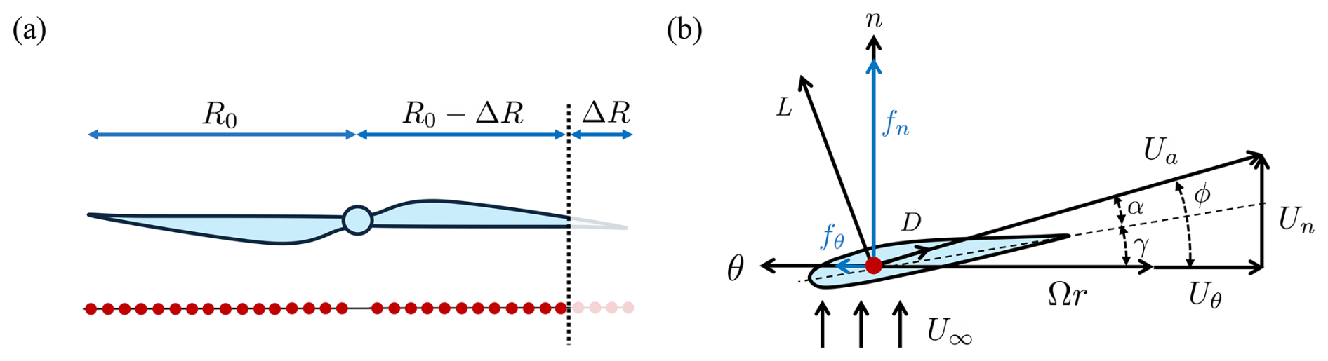
Figure 1 Illustration of the actuator line method (ALM) used in this study. (a) An asymmetric rotor is modeled by blade truncation, with definitions of the unmodified blade length R₀ and truncated blade length ΔR. The horizontal lines with a series of dots schematically show the un-truncated and truncated actuator lines, where each red dot represents an actuator element. (b) The velocity triangle illustrates the forces exerted by an actuator element. An airfoil cross-section is superimposed to enhance the clarity of the diagram.

As depicted in Fig. 1b, the apparent wind speed seen by an actuator element is $U_{\mathrm{a}}=\sqrt{U_n^{\mathrm{2}}+(U_{\mathit{\theta }}+\mathrm{\Omega }r{)}^{\mathrm{2}}}$, where U_n and U_θ are the axial and tangential velocity components, respectively. Ω is the rotor rotation speed, and r is the radial position of the blade element. The angle of attack is $\mathit{\alpha }=\mathit{\varphi }-\mathit{\gamma }$, and the inflow angle is $\mathit{\varphi }=\arctan \left(\frac{U_n}{U_{\mathit{\theta }}+\mathrm{\Omega }r}\right)$. γ is the local pitch angle. Here, c represents the chord length, while C_L(α) and C_D(α) are the lift and drag coefficients, respectively, determined by the tabulated airfoil polar data. The unit vectors e_L and e_D denote the directions of the lift and drag forces, respectively.

The resultant sectional forces are then projected onto the flow field as body forces using a 3D Gaussian regularization kernel η_ϵ to avoid spatial singularities (Sørensen and Shen, 2002), as written in Eq. (4).

$$\begin{array}{ll}{\displaystyle }& {\displaystyle }{\mathit{f}}_{\text{body}}\left(\mathit{x}\right)=\sum _{p=\mathrm{1}}^{N_b}\sum _{q=\mathrm{1}}^{N_{\text{AL}}}{F}_{\mathrm{1}}(r_{p,q}/R_{\mathrm{0}}){\mathit{f}}_{\mathrm{2}\mathrm{D}}\left({\mathit{r}}_{\mathit{p}\mathbf{,}\mathit{q}}\right){\mathit{\eta }}_{\mathit{ϵ}}\left(\right|{\mathit{r}}_{\mathit{p}\mathbf{,}\mathit{q}}-\mathit{x}\left|\right){\mathrm{\Delta }}_{\text{AL}},\\ \text{(4)}& {\displaystyle }& {\displaystyle }{\mathit{\eta }}_{\mathit{ϵ}}\left(d\right)={\displaystyle \frac{\mathrm{1}}{{\mathit{ϵ}}^{\mathrm{3}}{\mathit{\pi }}^{\mathrm{3}/\mathrm{2}}}}{\mathrm{e}}^{-(d/\mathit{ϵ}{)}^{\mathrm{2}}}\end{array}$$

Here, x denotes the position vector of the point of interest, and r_p,q denotes the position vector of the qth actuator line element of the pth blade. N_b and N_AL are the number of blades and number of actuator line elements per blade, respectively, and Δ_AL is the blade span that an actuator line element accounts for. $F_{\mathrm{1}}(r/R)$ represents the Shen correction factor (Shen et al., 2005), which is employed to account for the over-prediction of the blade tip load (Sarlak et al., 2016; Sørensen et al., 2016). η_ϵ(d) is the regularization kernel. This kernel controls the distribution of the force field based on the smoothing factor, denoted as ϵ, and the distance from an actuator element to x, denoted as d.

The ALM is implemented with the module turbinesFoam, developed by Bachant et al. (2019). As pointed out by Jha et al. (2014), three of the most important ALM parameters are grid spacing Δ, smoothing factor ϵ, and the discretization of the actuator line Δ_AL. Note that sensitivity tests of Δ and ϵ are provided in Sect. 4. First, the blade is discretized into 40 actuator line elements per blade with a uniform spacing Δ_AL. Notice that with these settings, Δ_AL is very close to Δ, which ensures that the force distributions are continuous along the blades (Martínez-Tossas et al., 2015). Then, following the recommendation of Troldborg (2009), ϵ=2Δ is set for the smoothing factor as a compromise that mitigates numerical oscillations while keeping the force concentrated, both of which significantly influence the structure of tip vortices.

The NREL 5 MW baseline wind turbine (Jonkman et al., 2009) is chosen as the reference wind turbine for this study. Its original design features a three-bladed rotor, with a swept radius R₀=63 m. The rotor is set to operate at a tip speed ratio of $\mathrm{\Omega }{R}_{\mathrm{0}}/U_{\mathrm{\infty }}=\mathrm{7.0}$, and the aeroelasticity and controller are omitted for simplicity. To focus more specifically on vortex pairing phenomena, the number of blades is reduced to two, positioned directly opposite each other. While this modification impacts induction and overall rotor loading, the tip vortex pairing motion analysis remains valid as long as relevant parameters, namely, vortex separation distance and circulation, are controlled (Quaranta et al., 2019). Moreover, the tower, nacelle, and ground effects are neglected, ensuring that the only asymmetry present is from the blade length difference.

2.3 Blade truncation and effective diameter

The rotor asymmetry is achieved by introducing a blade length difference across the two blades. One of the blade lengths is truncated with a length of ΔR, while the other blade is left unmodified. The blade truncation is implemented in the ALM by removing a certain number of actuator line points at the tip, which is depicted in Fig. 1a. Based on the current discretization of the actuator line, removing each actuator line element will result in reducing the blade length by around 2.5 % of R₀. It should be noted that, as reported in Table 2, the circulation strengths Γ of the tip vortices are very similar between the truncated and un-truncated blades. This supports the idea that introducing a blade length difference by directly truncating the blade is a suitable method for the current study.

As one may have postulated, the overall power performance of the rotor decreases by truncating one blade (see Table 1). Given that performance coefficients in wind energy fields are conventionally normalized by area, the effective swept area A_e is defined as the average of the original swept area, $\mathit{\pi }{R}_{\mathrm{0}}^{\mathrm{2}}$, and the area swept by the truncated blade, π(R₀−ΔR)². Consequently, the relations between R₀ and the effective swept area A_e, effective radius R_e, and effective diameter D_e can be derived as shown in Eq. (5). In this work, the effective diameter D_e serves as a bulk length scale for wake statistics, while D₀=2R₀ is used for analyzing tip vortex behavior, reflecting the physical position.

$$\begin{array}{ll}{\displaystyle }& {\displaystyle }{A}_{\mathrm{e}}=\mathit{\pi }{R}_{\mathrm{0}}^{\mathrm{2}}\left(\mathrm{1}-{\displaystyle \frac{\mathrm{\Delta }R}{R_{\mathrm{0}}}}+{\displaystyle \frac{\mathrm{1}}{\mathrm{2}}}{\left({\displaystyle \frac{\mathrm{\Delta }R}{R_{\mathrm{0}}}}\right)}^{\mathrm{2}}\right),\\ \text{(5)}& {\displaystyle }& {\displaystyle }{R}_{\mathrm{e}}=R_{\mathrm{0}}\sqrt{\mathrm{1}-{\displaystyle \frac{\mathrm{\Delta }R}{R_{\mathrm{0}}}}+{\displaystyle \frac{\mathrm{1}}{\mathrm{2}}}{\left({\displaystyle \frac{\mathrm{\Delta }R}{R_{\mathrm{0}}}}\right)}^{\mathrm{2}}},D_{\mathrm{e}}=\mathrm{2}{R}_{\mathrm{e}}\end{array}$$

Table 1 The main test matrix of the current study. Columns from left to right indicate the case name, inflow turbulence intensity TI (see Eq. 6), mesh resolution, blade length difference ΔR, effective rotor diameter D_e (see Eq. 5), thrust coefficient C_T, power coefficient C_P, effective thrust coefficient C_T,e, and effective power coefficient C_P,e (see Eq. 12). Case names follow a convention, starting with a prefix indicating the inflow conditions, followed by two digits representing the percentage of blade length difference, and having a postfix denoting the mesh resolution. The prefixes Lam, LT, and T correspond to laminar, low-turbulent, and turbulent inflow conditions, respectively. The postfixes S and D refer to the standard ($\mathrm{\Delta }=D_{\mathrm{0}}/\mathrm{80}$) and dense ($\mathrm{\Delta }=D_{\mathrm{0}}/\mathrm{160}$) mesh configurations, respectively.

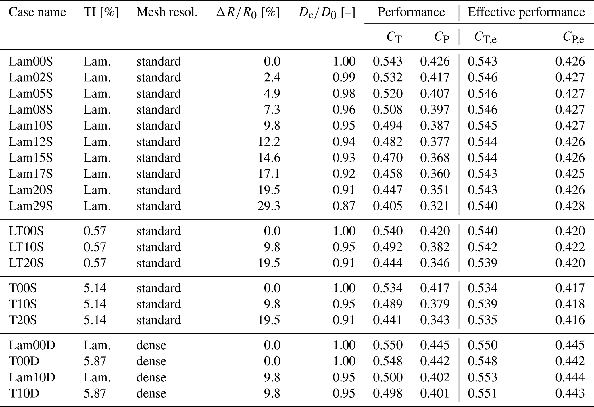
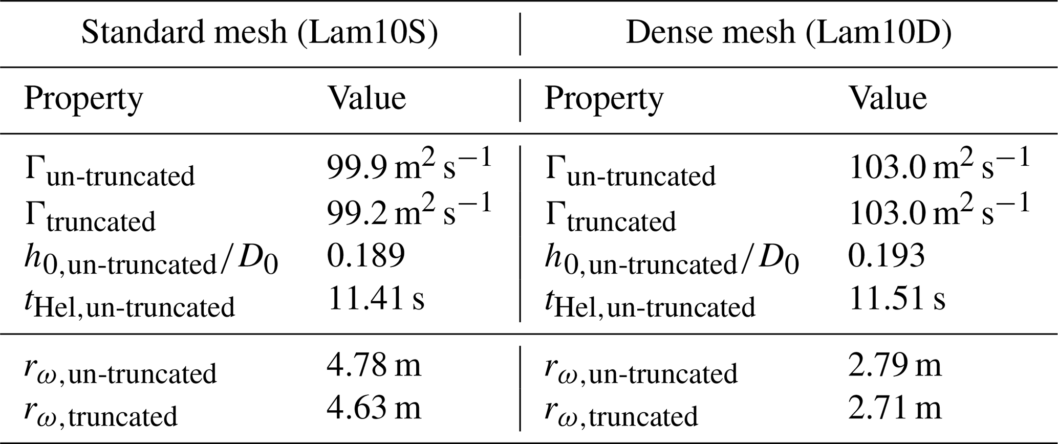
Table 2 Characteristic quantities of the vortices, measured when the vortex age corresponds to half a rotational period, as indicated by the magenta circles in Fig. 10. The parameter h₀ is determined based on the streamwise separation between the rotor plane and the centroid of the vortex of interest, and the vortex core size r_ω is determined by the tangential velocity profile (see Sect. 4). Note that for all LES-based analyses in this study, the values of h₀, Γ, and t_Hel are taken from the un-truncated blade in the case with $\mathrm{\Delta }R/R_{\mathrm{0}}\simeq \mathrm{10}\mathrm{\%}$ under laminar inflow conditions with the standard mesh (Lam10S). Notice that $t_{\text{Hel}}\equiv \mathrm{2}{h}_{\mathrm{0}}^{\mathrm{2}}/\mathrm{\Gamma }$.

2.4 Simulation setups

The simulation setups employed in this study largely follow those used by Li (2023) and Li et al. (2024), which have been validated and benchmarked against other independent experimental and numerical studies.

2.4.1 Grid layouts

For the laminar inflow cases, the computational domain is set to $\mathrm{12.5}{D}_{\mathrm{0}}\times \mathrm{5}{D}_{\mathrm{0}}\times \mathrm{5}{D}_{\mathrm{0}}$ in the x (streamwise), y (spanwise), and z (vertical) directions, respectively, as in the work of Li et al. (2024). A sensitivity test on the ratio of the rotor-swept area to the domain's cross-section is carried out in Sect. 4.2, showing that the effects of blockage are minimal. The rotor center is placed at the origin and is 2.5D₀ downstream from the inflow boundary and centered in the yz plane, as indicated by the white line in Fig. 2b. Within this domain, levels of refined mesh are arranged in a cylindrical shape with diameters of 3D₀, 2D₀, and 1.44D₀ for different refinement levels, as shown in Fig. 2a. Grids are generated using the application snappyHexMesh, containing 10.6×10⁶ cubic cells. As for the cases with turbulent inflow, the domain extends to 6D₀ upstream from the wind turbine rotor, which is the origin, with a refined region at the inflow, resulting in 12.0×10⁶ cells (see Fig. 2c). This modification accounts for the development of the turbulent structures and helps mitigate undesired pressure fluctuations caused by the synthetic turbulent inlet. For both mesh layouts (Fig. 2b and c), the grid cell size is $\mathrm{\Delta }/R_{\mathrm{0}}=\mathrm{1}/\mathrm{5}$ (i.e., 12.6 m) at level 1. At the most refined level around the rotor, which is level 4, the grid refines to $\mathrm{\Delta }/R_{\mathrm{0}}=\mathrm{1}/\mathrm{40}$ (i.e., 1.6 m), which falls within the range suggested by Jha et al. (2014). Note that unless otherwise mentioned, Δ refers to the grid size at level 4 in the remaining part of the current work.

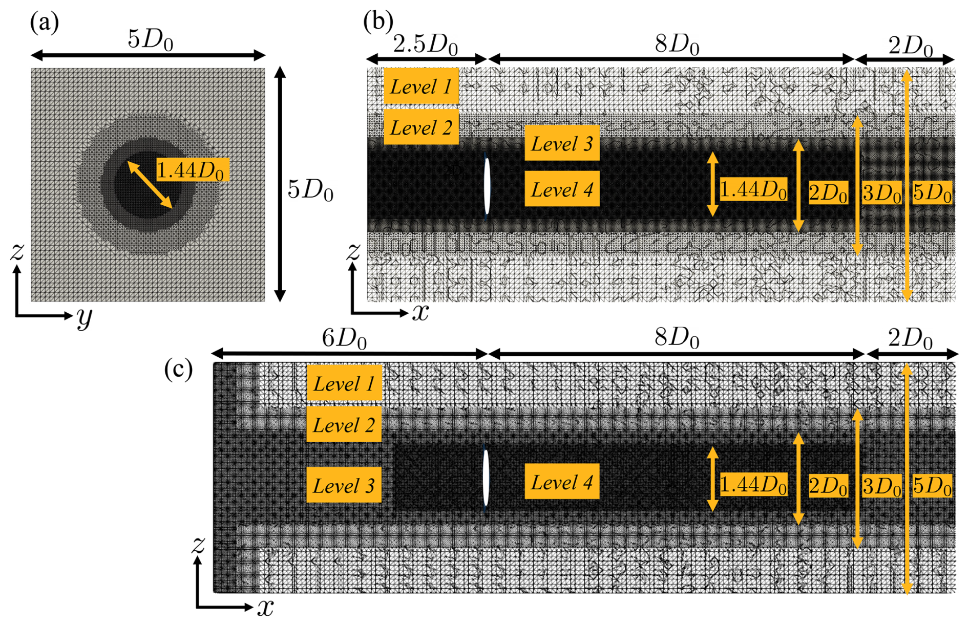
Figure 2 Mesh layouts for the simulation cases. (a) Cross-section at the rotor plane ($x/D_{\mathrm{0}}=\mathrm{0}$) for cases with both laminar and turbulent inflow conditions. Cross-section at $y/D_{\mathrm{0}}=\mathrm{0}$ (b) for laminar inflow cases and (c) for turbulent inflow cases. The white strips in (b) and (c) indicate the rotor position. The labels denote the different grid refinement levels.

2.4.2 Spatial and temporal discretization

The choice of spatial differencing scheme for the advective term influences energy dissipation levels and numerical stability in the simulation. It is well known that upwind schemes introduce numerical diffusion, whereas central difference schemes can lead to dispersion errors (Ferziger et al., 2002). To balance preserving wake structures and mitigating numerical oscillations, a blended scheme is employed (Gauss fixedBlended) (Ivanell et al., 2010; Jha et al., 2014). The composition of the scheme is 95 % fourth-order central difference scheme (cubic) and 5 % upwind scheme (upwind). The performance of the selected scheme is assessed and compared with several other common schemes in Appendix A.

The time step Δt is set at $\mathrm{1.4}\times {\mathrm{10}}^{-\mathrm{2}}$ s, corresponding to a one-degree rotor rotation. This ensures that the distance traveled by the rotor tip is below a grid size per time step, which is around 0.7Δ with the current setups. Note that this Δt results in a Courant–Friedrichs–Lewy number of 0.09, which is well below 1. In the simulations, the pressure–velocity coupled system is solved iteratively with PISO (Pressure Implicit with Splitting of Operators) algorithm. The time marching scheme employed is the Crank–Nicolson method with a coefficient of 0.9 (Crank--Nicolson 0.9). The simulations are conducted for 75 and 170 rotor revolutions for the cases subjected to laminar and turbulent inflow conditions, respectively, corresponding to approximately 375 and 850 s. Statistical data are collected after the 70th revolution to eliminate the influence of initial transients. The corresponding sampling windows are five revolutions for the laminar cases and 100 revolutions for the turbulent cases. Li et al. (2024) have demonstrated that these sampling durations are sufficient to achieve convergence of the second-order statistics.

2.4.3 Boundary condition

For the cases subjected to laminar inflow, the inflow conditions are specified as Dirichlet, with the velocity set at U_∞=11.4 m s⁻¹ and no velocity shear imposed. Slip conditions are applied at the boundaries on all four sides. At the outlet, an advective outflow condition, $D/Dt=\mathrm{0}$, is imposed to ensure mass conservation and to prevent distortion of the flow structures near the outlet (Troldborg, 2009).

In addition to the inflow conditions, the cases subjected to turbulent inflow conditions share the same boundary conditions as those with laminar inflow. To introduce inflow turbulence, the divergent-free synthetic eddy method (Poletto et al., 2013) is applied, which is implemented through turbulentDFSEMInlet. The time-averaged streamwise velocity profile is again uniformly set to U_∞=11.4 m s⁻¹. To characterize the strength of inflow turbulence intensity TI, it is measured at 2D₀ upstream from the rotor, using more than 40 probes. Additionally, the turbulence spectrum obtained is Kolmogorov-like, similar to those reported by Li et al. (2024). The definition of TI is given in Eq. (6), where σ_u, σ_v, and σ_w are the standard deviations of u, v, and w with respect to time. Two turbulence intensity levels are tested, which are a minor level (∼0.5 %) and an atmospheric boundary layer level (∼5 %). The former represents flow conditions typically encountered in controlled wind or water tunnels (Lignarolo et al., 2014; Quaranta et al., 2015), while the latter corresponds to typical inflow conditions for offshore wind farms (Troldborg et al., 2011; Hansen et al., 2012).

$$\begin{array}{}\text{(6)}& {\displaystyle }{\displaystyle }\text{TI}={\displaystyle \frac{\sqrt{\frac{\mathrm{1}}{\mathrm{3}}({\mathit{\sigma }}_u^{\mathrm{2}}+{\mathit{\sigma }}_v^{\mathrm{2}}+{\mathit{\sigma }}_w^{\mathrm{2}})}}{U_{\mathrm{\infty }}}}\times \mathrm{100}\mathrm{\%}\end{array}$$

In addition to closely matching the turbulence intensity typically found in controlled wind or water channel experiments, conditions with TI<1 % are also of interest for other reasons. Although these levels are significantly lower than those observed in typical offshore environments, previous numerical studies (Sarlak, 2014) have shown that even weak turbulence (TI≤0.5 %) can trigger instabilities that lead to wake breakdown, which is not observed with perfectly laminar inflow. Motivated by these findings, the present study also investigates whether ambient turbulence at such low levels influences leapfrogging instability and, in turn, affects the wake structure of an asymmetric rotor, with the aim of developing a more comprehensive understanding of the impacts of ambient turbulence.

2.4.4 Setups with a denser grid

In addition to the setups described earlier in this section, referred to as the “standard” setups (see Table 1), cases with denser grids are also tested, which are the “dense” cases. In general, the setups for the dense cases follow the same structures as for the standard cases, but the grid size Δ is halved. Specifically, $\mathrm{\Delta }=D_{\mathrm{0}}/\mathrm{160}$ (i.e., 0.8 m) is achieved at level 4 in Fig. 2. This results in the cell count for the laminar and turbulent cases reaching 85.4 and 96.1×10⁶, respectively. Additionally, the time step size Δt for the dense cases is also halved to ensure that the distance that the tip travels per time step is less than one grid. Thus, for the dense case, ΩΔt=0.5°. As one might expect, halving the cell size Δ increases the required CPU hours by approximately 16 times and the required memory by approximately 8 times. Therefore, cases with even finer mesh become unfeasible with the available computational resources.

Running simulations with higher mesh resolution is expected to capture finer details, particularly for modeling the vortex core size r_ω, which is crucial in terms of vortex dynamics (Cerretelli and Williamson, 2003; Leweke et al., 2016). Indeed, the numerical results of Selçuk et al. (2017) demonstrated that the detailed dynamics of the tip vortices of a two-bladed asymmetric rotor are affected by the vortex core radius when $r_{\mathit{\omega }}/R_{\mathrm{0}}$ falls between 0.03 and 0.10. Moreover, the overview provided by Abraham et al. (2023a) indicates that r_ω for rotors used for common industrial applications is around $\mathrm{1}\times {\mathrm{10}}^{-\mathrm{2}}{R}_{\mathrm{0}}$ to $\mathrm{5}\times {\mathrm{10}}^{-\mathrm{2}}{R}_{\mathrm{0}}$. However, to the authors' best knowledge, the precise vortex core size of a large-scale wind turbine (≥5 MW) is currently not publicly available.

Currently, r_ω found in the simulations is $\mathrm{7.6}\times {\mathrm{10}}^{-\mathrm{2}}{R}_{\mathrm{0}}$ with the standard mesh and $\mathrm{4.4}\times {\mathrm{10}}^{-\mathrm{2}}{R}_{\mathrm{0}}$ with the dense mesh (see Fig. 18). This indicates that the current setups for standard mesh can marginally meet the resolution requirements to properly capture the vortex cores of an industrial rotor, whereas the cases with the dense mesh are considered to have adequate resolution. However, experimental data from Ramos-García et al. (2023) indicate that tip vortex core sizes are around 0.11c_tip (c_tip is the chord length at the rotor tip) for the Joukowsky rotor (designed to have a constant circulation profile along the entire blade and thus having concentrated tip vortices) they used, and this value is equivalent to $\mathrm{1.4}\times {\mathrm{10}}^{-\mathrm{2}}{R}_{\mathrm{0}}$. For the NREL 5 MW turbine used in this study, 0.11c_tip corresponds to approximately $\mathrm{1.3}\times {\mathrm{10}}^{-\mathrm{3}}{R}_{\mathrm{0}}$ (c_tip=0.75 m; Jonkman et al., 2009), demonstrating that the vortex core size could be substantially smaller than what can be resolved in the current simulations. Despite this, the numerical results of Ramos-García et al. (2023) showed that the predicted leapfrogging distance closely matched experimental observations with a grid size of 4r_ω. This finding suggests that precisely capturing the vortex core size may not be necessary to predict the leapfrog instability, and this also agrees with the findings of Abraham et al. (2023a). In the present study, the leapfrogging distances predicted by the standard and dense setups are comparable, and the main conclusions remain consistent despite the predicted values of r_ω being significantly different (see Figs. 14 and 18). Therefore, this work primarily focuses on results obtained using the standard setup, while results from the dense setup are also frequently included in the discussion to further examine the effects of vortex core size on the detailed tip vortex dynamics.

2.5 Two-dimensional point vortex model and the definition of leapfrogging instability

To provide deeper insight, the simulation results from this study are compared with theoretical predictions of leapfrogging instability. Various approaches have been proposed in the literature to analyze this phenomenon and define its growth rate. Studies by Widnall (1972), Gupta and Loewy (1974), Ivanell et al. (2010), and Sarmast et al. (2014) have investigated the relevant instability modes in the frequency domain, while Bolnot (2012), Quaranta et al. (2019), Selçuk et al. (2017), and Delbende et al. (2021) have focused on time-domain analyses. The present study similarly evaluates the growth rate in the time domain. For comparison, the growth rates derived from LES data are assessed alongside predictions from a simplified model based on the framework proposed by Delbende et al. (2021), in which the tip vortex dynamics of an asymmetric rotor are captured using a simplified dynamical system.

2.5.1 Model definition

The 2D point vortex model used in this study is based on the framework established by Delbende et al. (2021), which reduces the complex helical tip vortex system of a two-bladed asymmetric rotor to two infinite arrays of point vortices, separated by a radial distance δr. This self-repeating vortex arrangement is schematically illustrated in Fig. 3, where the x and z axes correspond to the streamwise and radial directions of the helical system, respectively. Initially, the vortices within each array are evenly spaced by a distance of 2h₀ to replicate the helical pitch, with δr set equal to ΔR to represent the blade length difference. The two vortex arrays are staggered, with each vortex positioned midway between two adjacent vortices in the opposite array.

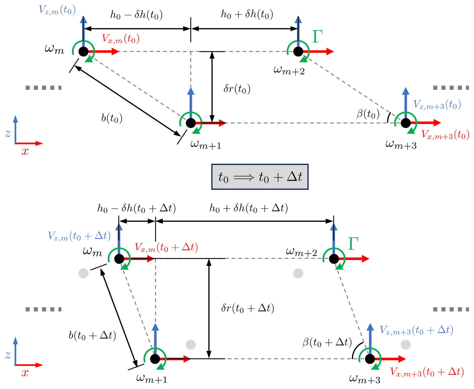
Figure 3 Schematic diagram illustrating the temporal evolution of self-repeating point vortex arrays from t₀ to t₀+Δt. The point vortices are labeled as ω_n ($n=m,m\pm \mathrm{1},m\pm \mathrm{2},\mathrm{\dots }$), with their induced velocities V_x,n and V_z,n shown by red and blue arrows, respectively. All vortices share the same circulation Γ, indicated by green circular arrows. Black solid circles represent the positions of the nth point vortex at the given time, while gray solid circles indicate their initial positions at t=t₀. Initially, neighboring vortices are spaced by h₀ in the x direction and by ΔR in the z direction, with δh(t₀)=0 and δr(t₀)=ΔR (upper diagram). Under induction from surrounding vortices, each ω_n is displaced by these induced velocities over a time step Δt (lower diagram). Note that δh and δr evolve over time, and β is defined as $\arctan (\mathit{\delta }r/(h_{\mathrm{0}}-\mathit{\delta }h\left)\right)$.

The dynamics of the mth vortex, marked as ω_m, is represented by its temporal displacement rates in the x and z directions ($\mathrm{d}{x}_m/\mathrm{d}t$ and $\mathrm{d}{z}_m/\mathrm{d}t$, where x_m and z_m are the x and z positions of ω_m), which are determined by the velocities V_x,m and V_z,m. These velocities are the sums of the induction from all other vortices (Anderson, 2017), as formulated in Eq. (7). The circulation Γ is assumed to be constant across both vortex arrays, and the index n ranges from −∞ to ∞, as the vortex arrays extend infinitely in the ±x directions.

$$\begin{array}{ll}{\displaystyle \frac{\mathrm{d}}{\mathrm{d}t}}\left[\begin{array}{c}{x}_m\\ z_m\end{array}\right]& {\displaystyle }=\left[\begin{array}{c}{V}_{m,x}\\ V_{m,z}\end{array}\right]\\ \text{(7)}& {\displaystyle }& {\displaystyle }=\left[\begin{array}{c}\frac{\mathrm{\Gamma }}{\mathrm{2}\mathit{\pi }}{\sum }_{n=-\mathrm{\infty },n\ne m}^{\mathrm{\infty }}\frac{z_n-z_m}{(x_n-x_m{)}^{\mathrm{2}}+(z_n-z_m{)}^{\mathrm{2}}}\\ \frac{\mathrm{\Gamma }}{\mathrm{2}\mathit{\pi }}{\sum }_{n=-\mathrm{\infty },n\ne m}^{\mathrm{\infty }}\frac{x_n-x_m}{(x_n-x_m{)}^{\mathrm{2}}+(z_n-z_m{)}^{\mathrm{2}}}\end{array}\right]\end{array}$$

Due to the inversion symmetry and periodicity, the magnitude of the induced velocity is identical for both arrays and is uniform across all vortices, i.e., $\left|V_{n,x}\right|=V_x$ and $\left|V_{n,z}\right|=V_z$. Specifically, when Γ is positive in the y direction, ω_m and ω_m+2 in Fig. 3 travel with +V_x and +V_z, while ω_m+1 and ω_m+3 travel with −V_x and −V_z. This leads to the pairing motion of ω_m and ω_m+1. Consequently, the variations of the streamwise and radial separations between a vortex pair, denoted as δh and δr (see Fig. 3), change at rates of 2V_x and 2V_z. Furthermore, V_x and V_z can be completely described by δh and δr, as written in Eq. (8). Note that the infinite sums can be expressed in closed algebraic expressions, and the detailed derivations can be found in the work of Delbende et al. (2021). The main advantage offered by the formulation in Eq. (8) is that the synchronous displacement across the vortex array ensures identical temporal evolution for any pair, thereby simplifying the study of vortex pairing growth rates to a single representative pair and reducing the system's degrees of freedom.

$$\begin{array}{ll}{\displaystyle \frac{\mathrm{d}}{\mathrm{d}t}}\left[\begin{array}{c}\mathit{\delta }h\left(t\right)\\ \mathit{\delta }r\left(t\right)\end{array}\right]& {\displaystyle }=\left[\begin{array}{c}\mathrm{2}{V}_x\left(\mathit{\delta }h\right(t),\mathit{\delta }r(t\left)\right)\\ \mathrm{2}{V}_z\left(\mathit{\delta }h\right(t),\mathit{\delta }r(t\left)\right)\end{array}\right]\\ {\displaystyle }& {\displaystyle }=\left[\begin{array}{c}\frac{\mathrm{\Gamma }}{\mathrm{2}\mathit{\pi }}{\sum }_{n=-\mathrm{\infty },n\notin \text{even}}^{\mathrm{\infty }}\frac{\mathit{\delta }r}{(x_n+n{h}_{\mathrm{0}}-\mathit{\delta }h{)}^{\mathrm{2}}+(\mathit{\delta }r{)}^{\mathrm{2}}}\\ \frac{\mathrm{\Gamma }}{\mathrm{2}\mathit{\pi }}{\sum }_{n=-\mathrm{\infty },n\notin \text{even}}^{\mathrm{\infty }}\frac{x_n+n{h}_{\mathrm{0}}-\mathit{\delta }h}{(x_n+n{h}_{\mathrm{0}}-\mathit{\delta }h{)}^{\mathrm{2}}+(\mathit{\delta }r{)}^{\mathrm{2}}}\end{array}\right]\\ {\displaystyle }& {\displaystyle }={\displaystyle \frac{\mathrm{\Gamma }}{\mathrm{2}{h}_{\mathrm{0}}}}\left[\begin{array}{c}\frac{\sinh \left(\mathit{\pi }\mathit{\delta }r/h_{\mathrm{0}}\right)}{\cos \left(\mathit{\pi }\mathit{\delta }h/h_{\mathrm{0}}\right)+\cosh \left(\mathit{\pi }\mathit{\delta }r/h_{\mathrm{0}}\right)}\\ \frac{\sin \left(\mathit{\pi }\mathit{\delta }h/h_{\mathrm{0}}\right)}{\cos \left(\mathit{\pi }\mathit{\delta }h/h_{\mathrm{0}}\right)+\cosh \left(\mathit{\pi }\mathit{\delta }r/h_{\mathrm{0}}\right)}\end{array}\right]\\ \text{(8)}& {\displaystyle }& {\displaystyle }\equiv {\displaystyle \frac{\mathrm{\Gamma }}{\mathrm{2}{h}_{\mathrm{0}}}}\left[\begin{array}{c}{f}_{\mathit{\delta }h}\left(\mathit{\delta }h\right(t),\mathit{\delta }r(t\left)\right)\\ f_{\mathit{\delta }r}\left(\mathit{\delta }h\right(t),\mathit{\delta }r(t\left)\right)\end{array}\right]\end{array}$$

To find out how δh and δr evolve in time, the equations of motion for vortex arrays written in Eq. (8) are integrated in time numerically, as given in Eq. (9). It should be noted that with the definitions of δh and δr given in Fig. 3, $\mathrm{d}\mathit{\delta }h/\mathrm{d}t$ and $\mathrm{d}\mathit{\delta }r/\mathrm{d}t$ are both 0 when $\mathit{\delta }h=\mathit{\delta }r=\mathrm{0}$. Also, the initial conditions are given as δh=0 and δr=ΔR for the cases considered in this work. Notice that because ΔR≠0, $\mathrm{d}\mathit{\delta }h/\mathrm{d}t\ne \mathrm{0}$.

$$\begin{array}{ll}{\displaystyle }& {\displaystyle \frac{\mathrm{d}}{\mathrm{d}t}}\left[\begin{array}{c}\mathit{\delta }h\\ \mathit{\delta }r\end{array}\right]\equiv {\displaystyle \frac{\mathrm{\Gamma }}{\mathrm{2}{h}_{\mathrm{0}}}}\left[\begin{array}{c}{f}_{\mathit{\delta }h}(\mathit{\delta }h,\mathit{\delta }r)\\ f_{\mathit{\delta }r}(\mathit{\delta }h,\mathit{\delta }r)\end{array}\right]\stackrel{\text{Time integration}}{⟶}\left[\begin{array}{c}\mathit{\delta }h\left(t\right)\\ \mathit{\delta }r\left(t\right)\end{array}\right]\\ \text{(9)}& {\displaystyle }& {\displaystyle }={\displaystyle \frac{\mathrm{\Gamma }}{\mathrm{2}{h}_{\mathrm{0}}}}\left[\begin{array}{c}{\int }_{t_{\mathrm{0}}}^t{f}_{\mathit{\delta }h}\left(\mathit{\delta }h\right(t^{\prime }),\mathit{\delta }r(t^{\prime }\left)\right)\mathrm{d}{t}^{\prime }\\ {\int }_{t_{\mathrm{0}}}^t{f}_{\mathit{\delta }r}\left(\mathit{\delta }h\right(t^{\prime }),\mathit{\delta }r(t^{\prime }\left)\right)\mathrm{d}{t}^{\prime }\end{array}\right]+\left[\begin{array}{c}\mathit{\delta }h(t=t_{\mathrm{0}})\\ \mathit{\delta }r(t=t_{\mathrm{0}})\end{array}\right]\end{array}$$

2.5.2 Leapfrogging instability

As derived in Sect. 2.5.1, Eq. (8) describes the vortex pairing motion due to the misalignment of two vortex arrays of a non-linear system. As detailed in Appendix B, by applying a Taylor expansion, the system can be linearized, making it an eigenvalue problem. After solving the eigenvalue problem, an unstable mode with a growth rate of λ can be found, and its mode shape for [δh;δr] is [1;1]. Given the eigenvector obtained for the unstable mode, selecting the L1 norm of δh and δr as the parameter estimating the growth of the unstable mode becomes natural, where the L1 norm is denoted as $\left|\right|\mathit{\eta }|{|}_{\mathrm{1}}$. The definition of $\left|\right|\mathit{\eta }|{|}_{\mathrm{1}}$ is given in Eq. (10). Furthermore, the time evolution of the L1 norm, $\left|\right|\mathit{\eta }|{|}_{\mathrm{1}}$, is chosen to be the indicator of the leapfrogging growth rate. Note that by the initial conditions of this work, when ΔR>0, $\left|\right|\mathit{\eta }|{|}_{\mathrm{1}}/\mathrm{\Delta }R$ is expected to grow exponentially in time from unity according to the result after the linearization (see Appendix B), as shown in Eq. (11).

$$\begin{array}{}\text{(10)}& {\displaystyle }& {\displaystyle }\left|\right|\mathit{\eta }|{|}_{\mathrm{1}}\equiv |\mathit{\delta }h|+|\mathit{\delta }r|\text{(11)}& {\displaystyle }& {\displaystyle }\left|\right|\mathit{\eta }\left(t\right)|{|}_{\mathrm{1}}/\mathrm{\Delta }R\simeq {\mathrm{e}}^{\mathit{\lambda }t}\text{for large}t\end{array}$$

However, this linearization may not be valid when δh and δr deviate significantly from the point where the Taylor expansion is carried out, as the system is inherently non-linear. Additionally, Eq. (11) becomes inaccurate when $\mathrm{d}\mathit{\delta }h/\mathrm{d}t$ and/or $\mathrm{d}\mathit{\delta }r/\mathrm{d}t$ have large values at t=t₀ (see Appendix B for details). To address these limitations, instead of estimating the growth rate using the linearized system, it is derived based on $\left|\right|\mathit{\eta }|{|}_{\mathrm{1}}$ obtained through carrying out time integration in Eq. (9), which accounts for non-linear effects. Consequently, the growth rate determined via time integration, denoted as σ_2D, is preferred over that determined via the linearized equations, denoted as λ.

To give an example, Fig. 4 plots $\left|\right|\mathit{\eta }|{|}_{\mathrm{1}}$ obtained via the time integration method against time t for the case with $\mathrm{\Delta }R/R_{\mathrm{0}}=\mathrm{9.8}\mathrm{\%}$, where the values of h₀ and Γ are based on the un-truncated blade of case Lam10S reported in Table 2. An exponential growth of $\left|\right|\mathit{\eta }|{|}_{\mathrm{1}}$ is evident, as indicated by the linear region in the semi-logarithmic plot. Specifically, the range $\mathrm{0.6}\le t/t_{\text{Hel}}\le \mathrm{0.8}$ (where $t_{\text{Hel}}=\mathrm{2}{h}_{\mathrm{0}}^{\mathrm{2}}/\mathrm{\Gamma }$) gives the most stable exponential growth rate, and this time window is also applicable to the LES data presented in Sect. 3.2.3. Therefore, the slope of this part is chosen to define the growth rate of the leapfrogging instability, which is denoted as σ_2D. In general, σ_2D is greater than λ when ΔR>0 (see Fig. 13). Furthermore, the leapfrogging time t_LF, marked by the vertical dashed line in Fig. 4, corresponds to the moment when the vortex pair swaps their streamwise positions, which occurs when δh=h₀.

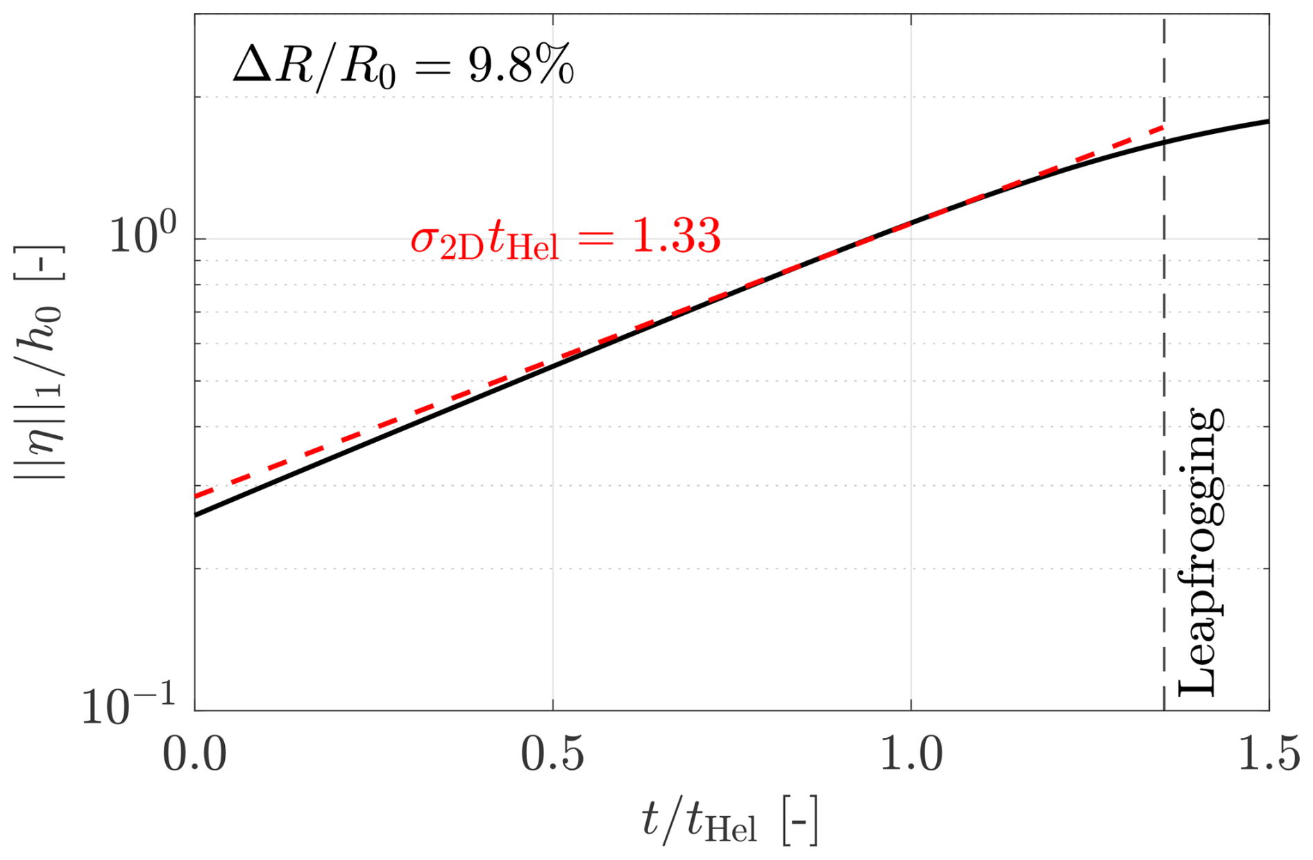
Figure 4 Temporal evolution of $\left|\right|\mathit{\eta }|{|}_{\mathrm{1}}$ obtained from the 2D vortex model with $\mathrm{\Delta }R/R_{\mathrm{0}}=\mathrm{9.8}\mathrm{\%}$. The values for h₀ and Γ are based on those in Table 2. The leapfrogging time t_LF is indicated by a vertical dashed line. Here, $\left|\right|\mathit{\eta }|{|}_{\mathrm{1}}=|\mathit{\delta }h|+|\mathit{\delta }r|$, and the characteristic helical timescale is $t_{\text{Hel}}=\mathrm{2}{h}_{\mathrm{0}}^{\mathrm{2}}/\mathrm{\Gamma }$.

In the results section (Sect. 3.2.3), the growth rate σ_2D obtained from the 2D model using the time integration method is compared with the LES results (σ_LES). This comparison evaluates whether the CFD results align with theoretical predictions. Additionally, following Quaranta et al. (2015), the characteristic timescale for the helical system of a two-bladed asymmetric rotor, denoted as t_Hel, is defined as $\mathrm{2}{h}_{\mathrm{0}}^{\mathrm{2}}/\mathrm{\Gamma }$. This timescale is commonly used in this study to normalize quantities related to growth rate and time.

2.6 Test matrix

In this work, simulations are conducted to investigate the effects of blade length difference ranging from 0.0 % to 30.0 % of R₀. Additionally, cases with varying inflow turbulence intensity (TI) are analyzed to assess the effects of ambient turbulence, specifically considering laminar, TI≃0.5 %, and TI≃5 %. Simulations with a finer mesh are also performed to examine the impact of mesh resolution. Furthermore, additional parametric studies exploring the effects of different simulation settings, including spatial discretization schemes, variations in the smoothing factor ϵ, and adjustments to the Smagorinsky constant C_s, are presented and discussed in Sect. 4.

The test matrix is presented in Table 1. The leftmost column lists the case name, followed by the inflow turbulence intensity TI and mesh resolution. Next, the blade length differences ΔR and the effective diameters D_e are given. Lastly, the corresponding (effective) thrust and power coefficients obtained from the LES-ALM results are included. For the effective performance coefficients, A_e is used for the normalization, as defined in Eq. (12). The consistency of the resulting C_T,e and C_P,e across cases with varying ΔR suggests that the proposed length scales, specifically R_e and D_e, are more appropriate for thrust- and power-related quantities. Notably, this also implies that D_e is preferred over D₀ when analyzing wake quantities, as these are mostly determined by the rotor performance.

$$\begin{array}{ll}{\displaystyle }& {\displaystyle }{C}_{\mathrm{T}}={\displaystyle \frac{\text{Thrust}}{\mathrm{0.5}\mathit{\rho }{U}_{\mathrm{\infty }}^{\mathrm{2}}\mathit{\pi }{R}_{\mathrm{0}}^{\mathrm{2}}}},C_{\mathrm{P}}={\displaystyle \frac{\text{Power}}{\mathrm{0.5}\mathit{\rho }{U}_{\mathrm{\infty }}^{\mathrm{3}}\mathit{\pi }{R}_{\mathrm{0}}^{\mathrm{2}}}},\\ \text{(12)}& {\displaystyle }& {\displaystyle }{C}_{\text{T,e}}={\displaystyle \frac{\text{Thrust}}{\mathrm{0.5}\mathit{\rho }{U}_{\mathrm{\infty }}^{\mathrm{2}}\mathit{\pi }{R}_{\mathrm{e}}^{\mathrm{2}}}},C_{\text{P,e}}={\displaystyle \frac{\text{Power}}{\mathrm{0.5}\mathit{\rho }{U}_{\mathrm{\infty }}^{\mathrm{3}}\mathit{\pi }{R}_{\mathrm{e}}^{\mathrm{2}}}},\end{array}$$

3 Results and discussion

In this section, the results are presented and discussed. Section 3.1 illustrates the dynamics of tip vortices using qualitative methods, specifically through contour plots of vorticity ω_y. Section 3.2 examines leapfrogging instability quantitatively, where vortex trajectories, leapfrogging growth rates obtained from LES data σ_LES, leapfrogging distance x_LF, and leapfrogging time t_LF are analyzed. Finally, Sect. 3.3 evaluates the impact of rotor asymmetry on integral wake characteristics, such as the area-averaged mean streamwise velocity, $\langle \stackrel{\mathrm{‾}}{u}{\rangle }_{\text{disk}}$.

3.1 Qualitative assessment of the tip vortices behavior

This subsection explores the dynamics of tip vortices in an asymmetric rotor using vorticity contour plots and three-dimensional iso-surfaces. Sect. 3.1.1 and 3.1.2 provide qualitative overviews of tip vortex behavior under laminar and turbulent inflow conditions, respectively. Additionally, Sect. 3.1.3 qualitatively examines the effects of mesh resolution on leapfrogging instability. Lastly, Sect. 3.1.4 demonstrates the three-dimensional vortical system of the asymmetric rotor studied in this work with iso-surfaces. Beyond the plots presented here, animations visualizing the time-evolving three-dimensional vortical structures for selected cases are available in the corresponding data repository (Yen et al., 2025).

3.1.1 Contours of tip vortices under laminar inflow

As shown in Fig. 5a, the contours of the instantaneous out-of-plane vorticity field (ω_y) reveal that tip vortices shed by a symmetric rotor ($\mathrm{\Delta }R/R_{\mathrm{0}}=\mathrm{0}\mathrm{\%}$) under laminar inflow conditions are convected downstream in a highly regular pattern. The consecutive tip vortices follow one another with minimal variation in the z direction (radial direction). Beyond approximately 4D₀ downstream, individual vortices become indistinguishable due to vortex diffusion, ultimately forming a stable vortex tube. Additionally, a shear layer is formed across this tube and extends beyond $x/D_{\mathrm{0}}=\mathrm{8}$ (see Figs. 5a and 15a). However, it is important to note that such conditions are unlikely to occur in practical wind farm environments, as perfectly turbulence-free inflow is unrealistic. Indeed, as shown in Fig. 6, even a minor level of inflow turbulence can trigger the wake breakdown process.

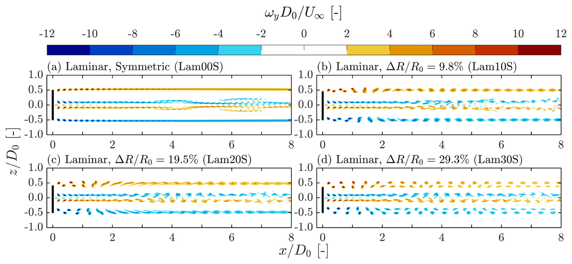
Figure 5 Contours of instantaneous out-of-plane vorticity ω_y for cases subjected to laminar inflow conditions with standard mesh and blade length differences of $\mathrm{\Delta }R/R_{\mathrm{0}}\simeq [\mathrm{0}\mathrm{\%},\mathrm{10}\mathrm{\%},\mathrm{20}\mathrm{\%},\mathrm{30}\mathrm{\%}]$. The corresponding ΔR values, together with their case names (see Table 1), are labeled at the top left of each panel. The black lines indicate the position of the rotor.

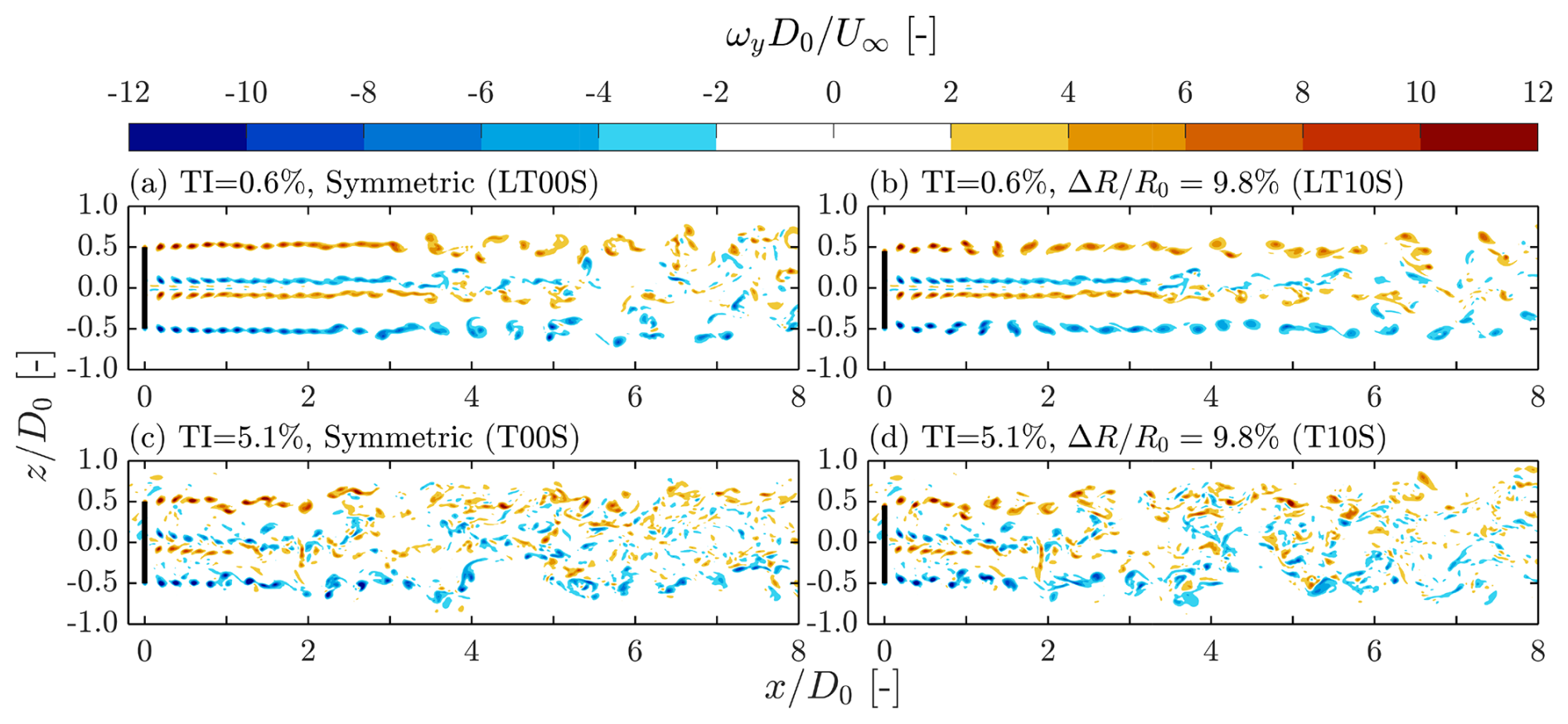
Figure 6 Contours of instantaneous out-of-plane vorticity ω_y for cases subjected to turbulent inflow conditions of $\text{TI}=[\mathrm{0.6}\mathrm{\%},\mathrm{5.1}\mathrm{\%}]$ with standard mesh and blade length differences of $\mathrm{\Delta }R/R_{\mathrm{0}}\simeq [\mathrm{0}\mathrm{\%},\mathrm{10}\mathrm{\%}]$. The corresponding TI and ΔR values, together with their case names (see Table 1), are labeled at the top left of each panel. The black lines indicate the position of the rotor.

Figure 5b presents the ω_y field for the case with a blade length difference of 9.8 % ($\mathrm{\Delta }R/R_{\mathrm{0}}\simeq \mathrm{10}\mathrm{\%}$). In this configuration, tip vortices are shed at different radial positions. Owing to the velocity differences that can be deduced from the Biot–Savart law, the outer vortices gradually overtake the inner ones. During this process, the vortices exhibit significant movement in the z direction (radial direction), and the streamwise spacing between consecutive vortices decreases. At approximately $x/D_{\mathrm{0}}=\mathrm{1.2}$, the outer vortex of a vortex pair overtakes the inner vortex (corresponding to δh=h₀, as defined in Fig. 3), marking the event of leapfrogging (further discussed in Sect. 3.2.3). During this overtaking event, both tip vortices deform from circular to elliptical shapes, which promotes vortex merging shortly after leapfrogging (Cerretelli and Williamson, 2003). Following the merging, a secondary helical vortex structure forms and remains stable beyond $x/D_{\mathrm{0}}=\mathrm{8}$.

The observed vortex pairing and merging under laminar inflow conditions are consistent with findings reported in the literature (Selçuk et al., 2017; Ramos-García et al., 2023). However, these results do not fully align with the predictions of Delbende et al. (2021). Under similar conditions ($h_{\mathrm{0}}/\mathit{\pi }{R}_{\mathrm{0}}<\mathrm{0.3}$ and $\mathrm{\Delta }R/R_{\mathrm{0}}<\mathrm{0.3}$), their inviscid vortex model predicts that outer vortices continuously overtake inner vortices without precession motions and merging. This discrepancy can be mainly attributed to the sizes of the vortex cores (Cerretelli and Williamson, 2003; Leweke et al., 2016), which is surveyed and discussed later on in Sects. 3.1.3 and 4.

For cases with larger blade length differences, the radial separation between the inner and outer vortices naturally increases. When the blade length difference reaches approximately 30 % (Fig. 5d), it is observed that after the first leapfrogging event (defined when δh=h₀), the outer vortices continuously overtake the inner vortices without merging. This behavior aligns with the predictions of Delbende et al. (2021). On the other hand, for a 20 % blade length difference (Fig. 5c), the tip vortex behavior falls between the cases observed for 10 % and 30 %. In this intermediate case, the inner tip vortices become sufficiently stretched such that portions of them merge with the outer vortices, while other segments continue to be overtaken within the range of $\mathrm{2}\le x/D_{\mathrm{0}}\le \mathrm{4}$. Another noteworthy observation is that larger values of $\mathrm{\Delta }R/R_{\mathrm{0}}$ cause the outer vortices to overtake the inner vortices at more upstream positions. For instance, overtaking occurs at approximately $x/D_{\mathrm{0}}\simeq \mathrm{1.2}$ for $\mathrm{\Delta }R/R_{\mathrm{0}}=\mathrm{10}\mathrm{\%}$ but shifts upstream to $x/D_{\mathrm{0}}\simeq \mathrm{1.0}$ for $\mathrm{\Delta }R/R_{\mathrm{0}}=\mathrm{20}\mathrm{\%}$ and 30 %.

Despite the occurrence of leapfrogging, the vorticity contours in Fig. 5b–d show that the wake structures remain relatively stable, with no signs of wake breakdown. This finding suggests that, under laminar inflow conditions, triggering the leapfrogging instability is not beneficial for enhancing wake recovery rates. This observation is further supported by the velocity field analyses presented later in Sect. 3.3.

3.1.2 Contours of tip vortices under turbulent inflow

In addition to laminar inflow conditions, this study also considers two levels of inflow turbulence intensities, which are TI=0.6 % and 5.1 %. Simulations are performed for both symmetric rotors and asymmetric rotors with varying blade length differences, as detailed in Table 1. However, for conciseness, this section focuses on the cases with $\mathrm{\Delta }R/R_{\mathrm{0}}=\mathrm{0}\mathrm{\%}$ and $\mathrm{\Delta }R/R_{\mathrm{0}}\simeq \mathrm{10}\mathrm{\%}$, as these configurations are the most representative of leapfrogging behavior, as evidenced by the vorticity contours in Fig. 5.

Figure 6a and b show the instantaneous vorticity field ω_y for cases with TI=0.6 %. For the symmetric rotor case, a comparison between Figs. 6a and 5a reveals that even a minor level of turbulence can trigger instabilities, including leapfrogging, ultimately leading to wake breakdown around $x/D_{\mathrm{0}}=\mathrm{4}$. This observation is consistent with experimental results from wind and water tunnel studies (Lignarolo et al., 2014; Quaranta et al., 2015), where inflow conditions exhibit very low TI but are not perfectly laminar. In contrast, for the asymmetric rotor case with $\mathrm{\Delta }R/R_{\mathrm{0}}\simeq \mathrm{10}\mathrm{\%}$, the tip vortex behavior remains largely unchanged between the laminar inflow case (Fig. 5b) and the case with TI=0.6 % (Fig. 6b) up to approximately $x/D_{\mathrm{0}}=\mathrm{5}$. This indicates that the low-level turbulence does not advance the leapfrogging event, a conclusion further supported by the leapfrogging distance analysis in Sect. 3.2.4. Additionally, the coherence of the vortex structures appears to be better maintained in the asymmetric rotor case, with the onset of wake breakdown delayed from approximately $x/D_{\mathrm{0}}=\mathrm{4}$ to $x/D_{\mathrm{0}}=\mathrm{5}$ compared to the symmetric rotor case. This observation is further validated by the phase-averaged vorticity magnitude $\stackrel{\mathrm{̃}}{\left|{\mathit{\omega }}_y\right|}$ presented later in Fig. 7.

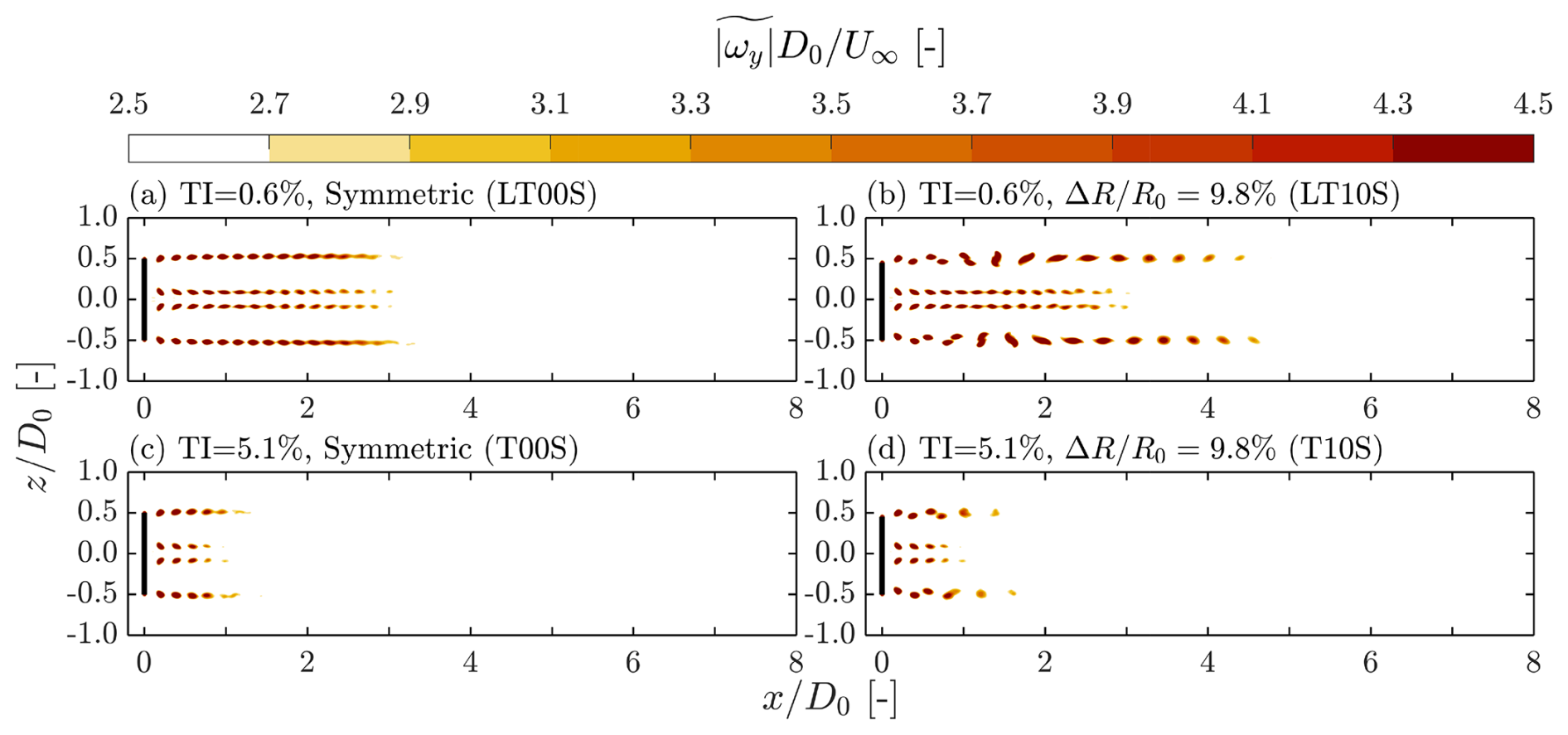
Figure 7 Contours of phase-averaged ω_y magnitude, denoted as $\stackrel{\mathrm{̃}}{\left|{\mathit{\omega }}_y\right|}$, for cases subjected to turbulent inflow conditions of $\text{TI}=[\mathrm{0.6}\mathrm{\%},\mathrm{5.1}\mathrm{\%}]$ with standard mesh and blade length differences of $\mathrm{\Delta }R/R_{\mathrm{0}}\simeq [\mathrm{0}\mathrm{\%},\mathrm{10}\mathrm{\%}]$. The corresponding TI and ΔR values, together with their case names (see Table 1), are labeled at the top left of each panel. The black lines indicate the position of the rotor.

The vorticity fields shown in Fig. 6c and d show that for cases with TI=5.1 %, the wake breakdown process initiates significantly earlier for both ΔR values compared to those with TI=0.6 %. In both the symmetric and asymmetric rotor cases, wake breakdown begins around $x/D_{\mathrm{0}}=\mathrm{1.5}$. Unlike the cases subjected to laminar and low-turbulence inflow conditions, the ω_y contours for these two cases become indistinguishable beyond approximately $x/D_{\mathrm{0}}=\mathrm{2}$. This demonstrates that, at this higher turbulence level, wake behavior is more strongly influenced by ambient turbulence rather than rotor asymmetry. This observation is further supported by the integral wake velocity analysis discussed in Sect. 3.3. However, in the very near wake region ($x/D_{\mathrm{0}}<\mathrm{1.5}$), the effects of ΔR remain identifiable. A visual inspection of the tip vortex patterns reveals that rotor asymmetry still promotes the leapfrogging phenomenon, a conclusion that will be more clearly demonstrated through the phase-averaged field presented in Fig. 7.

In addition to the instantaneous fields, phase-averaged contours of the out-of-plane vorticity magnitude $\stackrel{\mathrm{̃}}{\left|{\mathit{\omega }}_y\right|}$ are presented in Fig. 7. The phase-averaging procedure employed in this study is based on the rotor's rotational period, with the phase of interest corresponding to the position where one of the blades points in the positive z direction. Phase-averaged fields are particularly useful for assessing the coherence of periodically varying flow structures, such as those observed in wind turbine wakes (Li et al., 2024, 2025). It is important to note that $\stackrel{\mathrm{̃}}{\left|{\mathit{\omega }}_y\right|}$ contours for cases with laminar inflow conditions are not shown, as they are effectively identical to the instantaneous fields presented in Fig. 5 due to the strictly periodic nature of these systems.

Figure 7a and b present the $\stackrel{\mathrm{̃}}{\left|{\mathit{\omega }}_y\right|}$ fields for the cases with a symmetric and an asymmetric rotor when TI=0.6 %. After phase-averaging, the vortical structures observed in both cases with TI=0.6 % become more similar to the ω_y fields observed under laminar inflow conditions. The disappearance of the structures having concentrated $\stackrel{\mathrm{̃}}{\left|{\mathit{\omega }}_y\right|}$ indicates the onset of wake breakdown, as this suggests randomization in the positions of the vortices. A particularly interesting observation is that the vortical structures in the asymmetric rotor case appear slightly more coherent than those in the symmetric rotor case, suggesting that the introduced rotor asymmetries slightly delay the breakdown process. Specifically, clear vortex contours persist up to approximately $x/D_{\mathrm{0}}\simeq \mathrm{5}$ in the asymmetric rotor case, whereas they dissipate around $x/D_{\mathrm{0}}\simeq \mathrm{3}$ in the symmetric case. This enhanced coherence may be attributed to the merging process, which increases the circulation strength of the resulting vortices. However, this increased coherence does not necessarily imply that rotor asymmetry has an adverse effect on wake recovery, as the swirling motions induced by stronger vortices may, in fact, enhance energy entrainment via advection (Li et al., 2024). After all, as shown in later sections, the wake recovery rates for cases with TI=0.6 % are largely unaffected by rotor asymmetry.

The contours of $\stackrel{\mathrm{̃}}{\left|{\mathit{\omega }}_y\right|}$ for the cases subjected to TI=5.1 % are shown in Fig. 7c and d. After phase-averaging, the leapfrogging event in the case with $\mathrm{\Delta }R/R_{\mathrm{0}}\simeq \mathrm{10}\mathrm{\%}$ becomes more clearly delineated compared to the instantaneous ω_y fields presented in Fig. 6d. Additionally, for the symmetric rotor case, the regular pattern of vortical structures is partially restored through phase-averaging. Similar to the observations at TI=0.6 %, the coherence of the vortical structures is enhanced by rotor asymmetry, although to a lesser extent at higher turbulence levels. Furthermore, unlike in the TI=0.6 % cases, where elevated values of $\stackrel{\mathrm{̃}}{\left|{\mathit{\omega }}_y\right|}$ persist beyond $x/D_{\mathrm{0}}=\mathrm{4.0}$, the regions of high $\stackrel{\mathrm{̃}}{\left|{\mathit{\omega }}_y\right|}$ for TI=5.1 % diminish rapidly, disappearing before $x/D_{\mathrm{0}}=\mathrm{1.5}$. These findings are consistent with the observations from the instantaneous fields and further demonstrate that, at higher turbulence intensities, ambient turbulence dominates the wake aerodynamics, making the effects of rotor asymmetries insignificant.

3.1.3 Contours of tip vortices with a higher mesh resolution

Contours of the instantaneous ω_y fields for the cases with a denser mesh listed in Table 1 are shown in Fig. 8. These cases include both symmetric and asymmetric rotor configurations ($\mathrm{\Delta }R/R_{\mathrm{0}}=\mathrm{9.8}\mathrm{\%}$), subjected to laminar and turbulent inflow conditions (TI=5.9 %). Despite the slight difference in TI between the cases subjected to turbulent inflow with two different mesh resolutions (TI=5.9 % for the dense resolution and 5.1 % for the standard resolution), they are directly compared, as the discrepancy in turbulence levels is considered small.

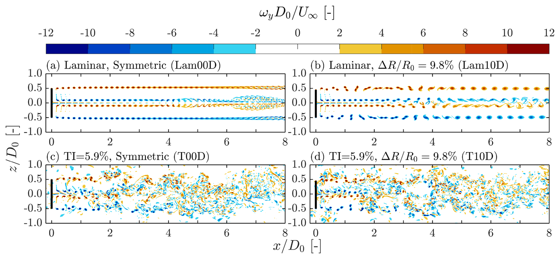
Figure 8 Contours of instantaneous out-of-plane vorticity ω_y for cases subjected to laminar and turbulent (TI=5.9 %) inflow conditions with dense mesh and blade length differences of $\mathrm{\Delta }R/R_{\mathrm{0}}\simeq [\mathrm{0}\mathrm{\%},\mathrm{10}\mathrm{\%}]$. The corresponding TI and ΔR values, together with their case names (see Table 1), are labeled at the top left of each panel. The black lines indicate the position of the rotor.

Focusing on the two cases subjected to laminar inflow (Fig. 8a and b), their overall features are consistent with those observed in the standard mesh cases (Fig. 5a and b). In particular, a stable vortex tube forms in the symmetric rotor case, while in the asymmetric rotor case, vortex pairs eventually merge to form a secondary helical structure. However, closer inspection reveals that the vortex cores in the denser mesh case (Lam10D) are smaller than those in the standard mesh case (Lam10S), and the consecutive vortices merge at a significantly later stage in both cases. Furthermore, for the asymmetric rotor configuration, the denser mesh case (Lam10D) exhibits a second leapfrogging event following the first, whereas this is not observed in the standard mesh case (Lam10S). This difference can be attributed to the larger vortex core size r_ω in Lam10S, which leads to earlier vortex merging (Selçuk et al., 2017), thereby naturally stopping the leapfrogging.

For the two cases subjected to turbulent inflow (Fig. 8c and d), differences in tip vortex dynamics compared to the standard mesh cases (Fig. 6c and d) are even less pronounced than those observed under laminar inflow conditions. The main distinctions introduced by the denser mesh are smaller vortex core sizes and more finely resolved turbulent structures. Additionally, the phase-averaged fields $\stackrel{\mathrm{̃}}{\left|{\mathit{\omega }}_y\right|}$ for the two turbulent cases with the dense mesh (not shown) closely resemble those obtained with the standard mesh (see Fig. 7c and d). These observations support the idea that the presence of atmospheric-level turbulence diminishes the influence of mesh resolution for the current application.

3.1.4 Three-dimensional vortical structures

Although the two-dimensional planes presented in Figs. 5 and 6 are able to effectively illustrate the vortical structures of an asymmetric rotor, some of their important three-dimensional traits are not clearly depicted. To better visualize the vorticity structures associated with the asymmetric rotor studied in this work, three-dimensional iso-surfaces of the instantaneous vorticity magnitude $\left|\mathit{\omega }\right|$ from case Lam10D are presented in Fig. 9. This case is highlighted because it is the only one that clearly exhibits two leapfrogging events, making it particularly illustrative for demonstrating the leapfrogging phenomenon. It should be noted that the case with the standard mesh (Lam10S) has very similar three-dimensional structures but with the merging happening earlier (see the supplementary animations Yen et al., 2025).

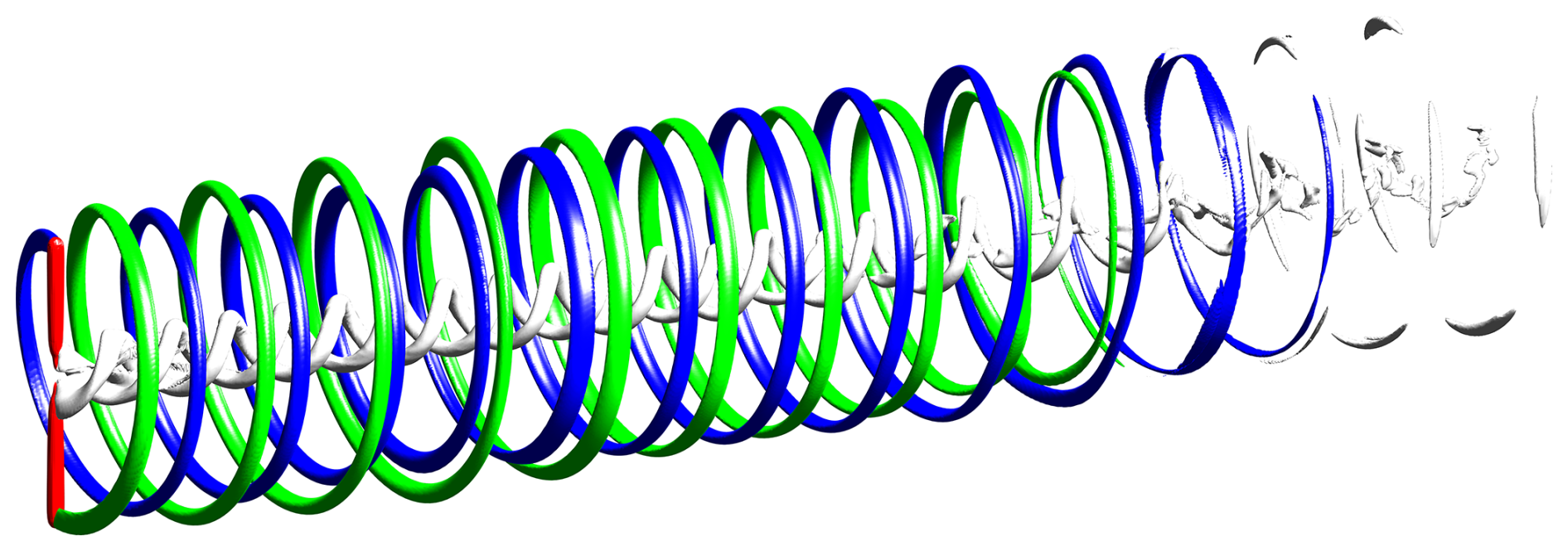
Figure 9 Three-dimensional iso-surfaces illustrating the vorticity structures of case Lam10D, shown when the truncated blade is oriented upward. The red surfaces represent the rotor, visualized using the magnitude of the body force field exerted by the actuator lines. Blue and green surfaces correspond to tip vortices shed from the truncated and un-truncated blades, respectively. Silver surfaces represent root vortices and tip vortices that are difficult to assign to a specific blade. The iso-value used for visualizing the vortices is $\left|\mathit{\omega }\right|D_{\mathrm{0}}/U_{\mathrm{\infty }}=\mathrm{10}$.

In Fig. 9, tip vortices shed by different blades are color-coded differently to enhance visualization. The interlaced helical structures are clearly visible, and the leapfrogging event can be easily identified as the tip vortices from different blades exchange their streamwise positions. Additionally, the figure shows that the radii of the helices vary as they undergo the leapfrogging process, which are features that may not be readily apparent from two-dimensional contour plots. Furthermore, Fig. 9 straightforwardly demonstrates that only global pairing modes are observed with the absence of local pairing modes, which is consistent with the findings of previous studies conducted under similar setups (Quaranta et al., 2015, 2019). Note that the absence of a local pairing mode holds for all cases subjected to laminar inflow conditions, as can be confirmed with the supplementary animations (Yen et al., 2025).

3.2 Quantification of leapfrogging instability

This subsection focuses on the leapfrogging phenomenon and its associated characteristics. Here, the trajectories of vortex pairs and the leapfrogging instability are captured quantitatively from the LES data. In addition, the leapfrogging distance x_LF and leapfrogging time t_LF are analyzed across various rotor asymmetries, inflow turbulence intensities (TI), and mesh resolutions. Furthermore, the obtained leapfrogging-related quantities are benchmarked against theoretical predictions and experimental outcomes.

3.2.1 Vortex identification and trajectory tracking

This part demonstrates how the positions and trajectories of the vortices are identified and tracked, forming the basis for determining the leapfrogging growth rate and leapfrogging distance. For brevity, only cases Lam10S and Lam10D from Table 1 are demonstrated, with a focus on illustrating the methodology for extracting leapfrogging-related quantities and highlighting the influence of mesh resolution.

To track the positions of the vortices, vortex centroids are defined at locations where local maxima of $\left|{\mathit{\omega }}_y\right|$ are detected at the initial time step, following the approach described by Troldborg (2009). Examples of detected vortex centroids are shown by the markers in Fig. 10a. The vortex trajectories are then obtained by tracking the temporal evolution of these centroids' positions using a technique similar to that employed in particle tracking velocimetry (Raffel et al., 2018). This method assumes that each vortex travels as a coherent structure and its centroid can always be identified. Starting from the initial positions of the most recently shed vortices, their motion is tracked by searching for the nearest neighbor within a defined radius around the predicted position in the subsequent time frame. This process is repeated until the vortex exits the domain of interest. The resulting trajectories for cases Lam10S and Lam10D (laminar inflow, $\mathrm{\Delta }R/R_{\mathrm{0}}\simeq \mathrm{10}\mathrm{\%}$, standard and dense mesh) are shown in Fig. 10b and d. These trajectories capture the spatiotemporal development of the vortex pairs, revealing their precessional (leapfrogging) motion.

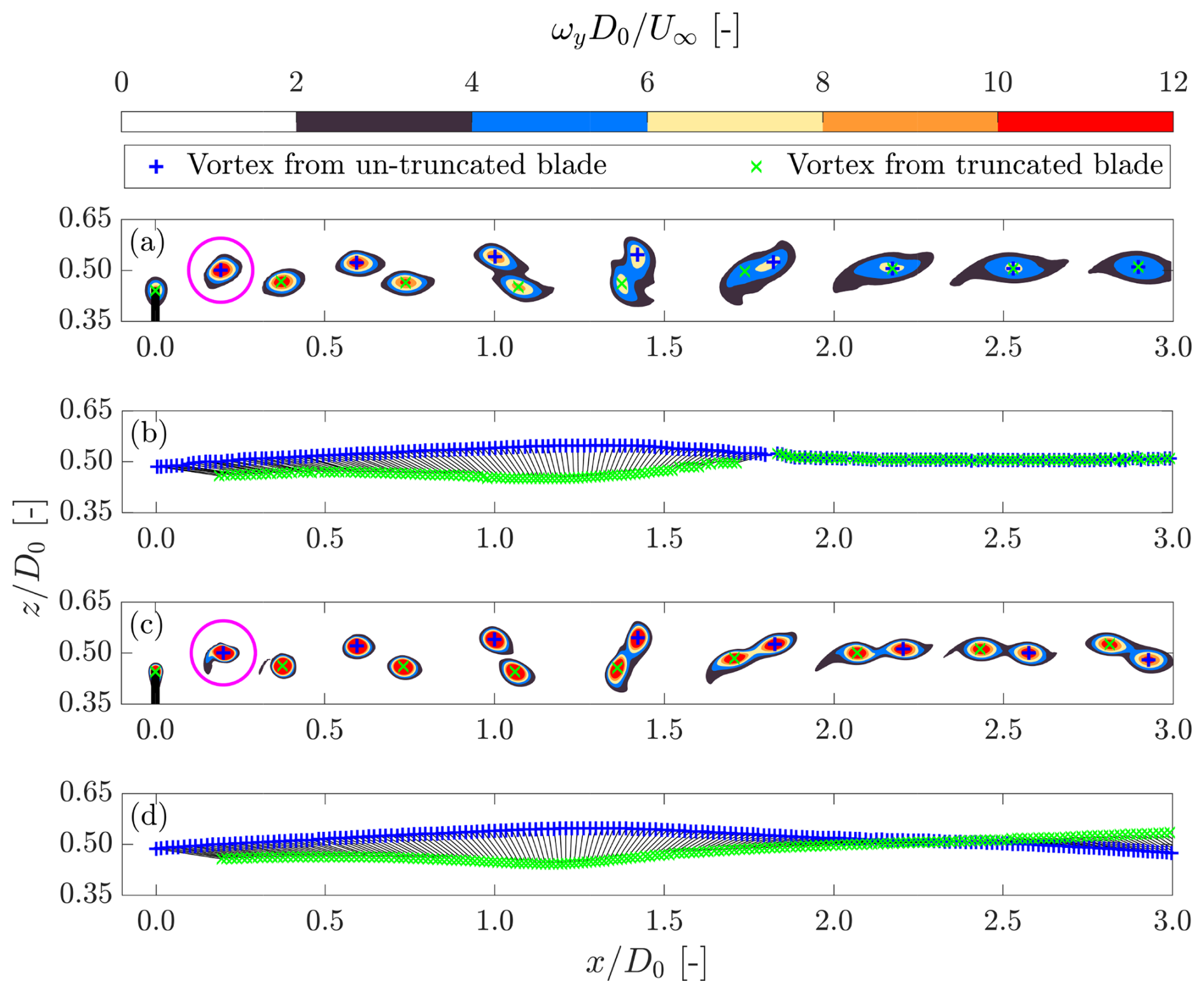
Figure 10 Demonstration of vortex pair tracking for cases with $\mathrm{\Delta }R/R_{\mathrm{0}}\simeq \mathrm{10}\mathrm{\%}$ using both the standard mesh (a, b, Lam10S) and the dense mesh (c, d, Lam10D). (a, c) Contours of ω_y near the tip height at the time instant when the truncated blade is oriented upward. Green crosses and blue pluses indicate the centroids of tip vortices shed from the truncated and unmodified blades, respectively. The black line denotes the rotor position. The magenta circles have a diameter of h₀ and are centered at the vortex centroids. (b, d) Trajectories of vortices released from the truncated blade (green crosses) and the unmodified blade (blue pluses). Black lines connecting the markers represent the separation vector b between the two vortices of each vortex pair.

The obtained trajectories (Fig. 10a and c) show good agreement with the corresponding ω_y contours presented in Figs. 5b and 8b. In both cases, the outer vortex (indicated by blue pluses) overtakes the inner vortex (indicated by green crosses) at approximately $x/D_{\mathrm{0}}=\mathrm{1.2}$. As previously noted, in the standard mesh case (Lam10S), the vortex pairs rapidly merge following their first leapfrogging event. In contrast, for the dense mesh case (Lam10D), the two vortices remain clearly distinguishable, and the onset of a second leapfrogging event is observed.

After capturing the vortex trajectories, key quantities, including the temporal evolution of the vortex pair's separation vector, can be extracted. These measurements are subsequently used to determine the leapfrogging distance x_LF, leapfrogging time t_LF, and leapfrogging growth rate σ_LES in the following sections.

3.2.2 Characteristic quantities related to the leapfrogging instability

Before analyzing the leapfrogging instability, two characteristic parameters, which are the initial streamwise spacing between consecutive vortices, h₀, and the circulation strength, Γ (see Fig. 3), are measured and reported in Table 2, along with the characteristic helical timescale $t_{\text{Hel}}\equiv \mathrm{2}{h}_{\mathrm{0}}^{\mathrm{2}}/\mathrm{\Gamma }$. Note that the vortex core size r_ω is also reported for completeness, which is determined based on the tangential velocity profile around the vortex centroid (see Sect. 4 for details). For consistency, all LESs in this study use the same values of h₀, Γ, and t_Hel, which are based on those of case Lam10S ($\mathrm{\Delta }R/R_{\mathrm{0}}\simeq \mathrm{10}\mathrm{\%}$, standard mesh, laminar inflow). That is, despite differences in rotor asymmetry, inflow conditions, and mesh resolutions, all cases share these characteristic parameters. Unless otherwise specified, h₀ and Γ are measured from the tip vortices shed by the un-truncated blade at the moment when the vortex age is half a rotor rotational period, which are those enclosed by the magenta circles in Fig. 10. In this work, h₀ is determined as the streamwise distance between that vortex centroid and the rotor plane, while Γ is obtained by evaluating a circular line integral having a diameter of h₀, centered on that vortex centroid in the y plane (Ramos-García et al., 2023). Also, note that torsional effects due to helical pitch are not accounted for in these measurements.

In Table 2, Γ and r_ω of the truncated blade are also measured at the moment when its vortex age is half a rotor rotational period. The results show that the relative difference in circulation strength between the truncated and un-truncated blades is within 1 % for both mesh resolutions, confirming that the assumption Γ_truncated=Γ_un-truncated holds fairly well. Additionally, relative differences between r_ω,truncated and r_{ω,un-truncated} are also merely around 3 %, further justifying the assumption that the tip vortices shed by the truncated and un-truncated blades are identical. Furthermore, the relative differences in h₀, Γ, and t_Hel between different mesh resolutions are approximately 2 %, 3 %, and 1 %, respectively. These small differences indicate that treating these parameters as constant across different mesh resolutions is well justified. On the other hand, a discussion on the differences in r_ω found in different mesh resolutions is provided in Sect. 4.

Following the notations defined in the 2D vortex model (see Fig. 3), the evolutions of the vortex pair for cases Lam10S and Lam10D are presented in Fig. 11. The angle between the vortex pair and the streamwise direction β, the separation distance b, the streamwise separation h₀−δh, and the radial separation δr are plotted against the streamwise location of the vortex pair's centroid (averaging the centroids of the two vortices).

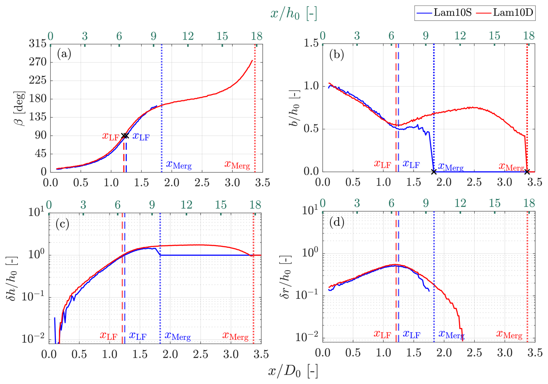
Figure 11 Evolution of the separation and orientation of a vortex pair for cases with $\mathrm{\Delta }R/R_{\mathrm{0}}\simeq \mathrm{10}\mathrm{\%}$ under laminar inflow conditions. Results are shown for both the standard mesh resolution (blue lines, Lam10S) and the dense mesh resolution (red lines, Lam10D). The definitions of β, b, δh, and δr are provided in Fig. 3.

In Fig. 11, both β and δh are observed to increase after the vortices are released from the rotor at $x/D_{\mathrm{0}}=\mathrm{0}$, indicating that the outer vortex of the pair gradually overtakes the inner vortex. When δh=h₀ and β=90°, the vortex pair becomes aligned in the radial direction, and the corresponding streamwise location is defined as the leapfrogging distance in this study, which is denoted as x_LF. Additionally, δr increases with x and reaches its maximum near x_LF. The decreasing trend of b before the leapfrogging event demonstrates that the vortices move closer together. At the moment when only a single vorticity peak is detected within the search radius, b is set to 0, indicating that the vortices have merged. Notably, before merging, only one leapfrogging event is identified in the case with the standard mesh, whereas two leapfrogging events are found in the case with the dense mesh, as indicated by β exceeding 270° prior to merging. This behavior is consistent with the contour plots shown previously (Figs. 5b and 8b) as well as the previous findings (Selçuk et al., 2017; Delbende et al., 2021), which show that the detail tip vortex dynamics after the first leapfrogging event, including the merging process, are sensitive to the vortex core size r_ω and fluid diffusivity.

For both cases, the initial value of δr is expected to match the imposed radial offset ΔR, which is 10 % of R₀, for the cases shown in Fig. 11. However, a discrepancy of approximately 0.04R₀ between the initial δr and the prescribed ΔR is observed. This deviation can likely be attributed to wake expansion. Specifically, by the time the subsequent vortex is shed from the un-truncated blade, the previously shed vortex from the truncated blade has already moved outward, reducing the effective radial separation between them. Additionally, the growth rate of δh is found to be nearly twice that of δr, deviating from the eigenvector prediction of [1;1] derived through linearization in Appendix B. This difference is likely due to the influence of initial conditions and the presence of non-linear effects in the vortex dynamics.

3.2.3 Leapfrogging instability growth rate

As defined in Sect. 2.5, the instability growth rate σ_LES is determined based on the L1 norm of the measured δh and δr, denoted as $\left|\right|\mathit{\eta }|{|}_{\mathrm{1}}$. Figure 12 presents a semi-log plot of $\left|\right|\mathit{\eta }|{|}_{\mathrm{1}}$ vs. time, with data from case Lam10S, case Lam10D, and the 2D vortex model. Overall, the σ_LES values obtained from the LES data show good agreement with the predictions of the 2D vortex model prior to the leapfrogging event. Moreover, the $\left|\right|\mathit{\eta }|{|}_{\mathrm{1}}$ curve for the case with the denser mesh (Lam10D) aligns more closely with the 2D vortex model results. This improved agreement is likely due to the smaller grid size Δ and reduced smoothing factor ϵ, which lead to smaller vortex core sizes r_ω and cause the vortices to behave more like idealized point vortices. Additionally, the smaller grid size reduces the subgrid-scale viscosity ν_sgs in Eq. (2), making the simulated flow more closely resemble the inviscid conditions, which is also a key assumption imposed by the 2D vortex model.

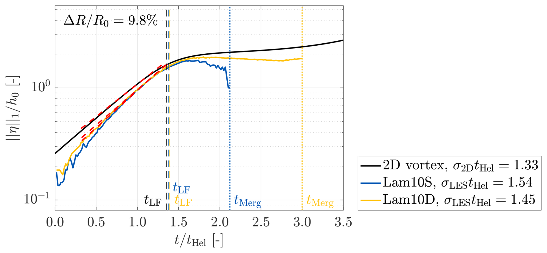
Figure 12 Temporal evolution of $\left|\right|\mathit{\eta }|{|}_{\mathrm{1}}$ obtained from the LESs using the standard mesh (blue line, Lam10S) and the dense mesh (yellow line, Lam10D), alongside the result from the 2D vortex model described in Sect. 2.5 (black line). The time of the first leapfrogging event (when β reaches 90°) is indicated by t_LF, and the time of vortex merging (when b reduces to 0) is marked as t_Merg. The growth rates are determined based on the slopes between 0.6 and 0.8t_LF, and these slopes are indicated by the red dashed lines.

A monotonic increase in $\left|\right|\mathit{\eta }|{|}_{\mathrm{1}}$ is observed before the leapfrogging time t_LF for both Lam10S and Lam10D. Furthermore, consistent with the behavior predicted by the 2D vortex model, distinct linear regions can be identified, indicating that $\left|\right|\mathit{\eta }|{|}_{\mathrm{1}}$ obtained from the LESs also grows exponentially with time. These linear segments enable the effective determination of the leapfrogging instability growth rate based on the slopes obtained from the LES data, denoted as σ_LES. Additionally, the curves in Fig. 12 show a transient phase that precedes the linear growth region, followed by a decrease in slope after the leapfrogging event. This behavior is in good agreement with the evolution of streamwise vortex separation documented in previous studies by Bolnot (2012) and Quaranta et al. (2019). For consistency, both σ_2D and σ_LES are determined based on the time interval $\mathrm{0.6}\le t/t_{\text{Hel}}\le \mathrm{0.8}$, during which the $\left|\right|\mathit{\eta }|{|}_{\mathrm{1}}$ curves exhibit the most stable exponential growth phase.

The growth rates σ_LES obtained under different inflow conditions and blade length differences (ΔR) are plotted in Fig. 13, accompanied by the σ_2D predicted by the 2D vortex model. For the turbulent inflow cases, the evaluation is based on 90–100 vortex pairs. The averages and standard errors of σ_LES are calculated, with the resulting 95 % confidence intervals being less than ±0.1 % for TI=0.6 % and up to ±9.7 % for TI=5.1 % relative to their respective means. It should be noted that leapfrogging events are not always detected for every vortex pair under turbulent inflow conditions. Specifically, for cases with $\mathrm{\Delta }R/R_{\mathrm{0}}\simeq \mathrm{10}\mathrm{\%}$, the detection rate of leapfrogging is approximately 97 % when TI=0.6 % and around 75 % when TI=5.1 %. In the instances where leapfrogging is not detected, the corresponding data are still included in the statistical analysis of σ_LES, but they are excluded from the calculations of leapfrogging time t_LF and leapfrogging distance x_LF.

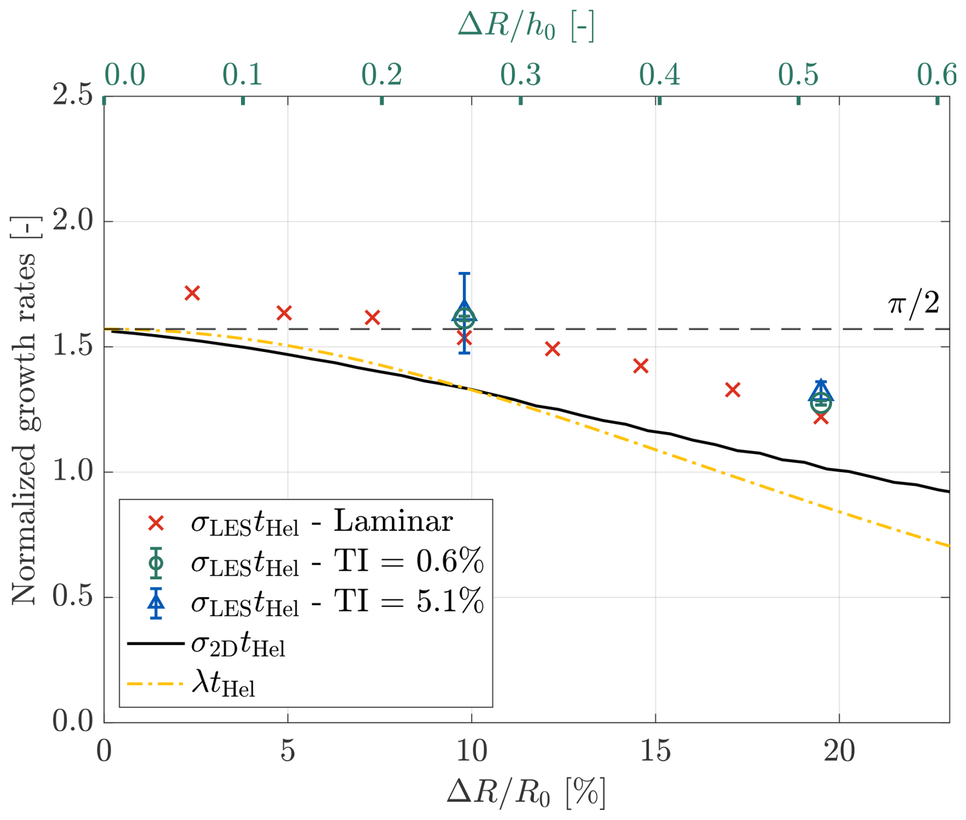
Figure 13 Comparison of growth rates obtained using different methods, including LESs with the standard mesh under various inflow conditions (σ_LES), the 2D vortex model described in Sect. 2.5 (σ_2D), and the linearized system derived in Appendix B (λ). Normalization of these quantities is done against $t_{\text{Hel}}^{-\mathrm{1}}=\mathrm{\Gamma }/\mathrm{2}{h}_{\mathrm{0}}^{\mathrm{2}}$. The normalized growth rates σ_LESt_Hel for the two dense-mesh cases with $\mathrm{\Delta }R/R_{\mathrm{0}}\simeq \mathrm{10}\mathrm{\%}$ are 1.45 for laminar inflow (Lam10D) and 1.61 for TI=5.9 % (T10D). These values are not plotted to avoid overcrowding the figure.

Under laminar inflow conditions, the normalized growth rates σ_LESt_Hel (represented by red crosses in Fig. 13) are observed to decrease with increasing ΔR, from 1.71 to 1.22. This trend aligns well with the predictions of the 2D vortex model, which drops from 1.53 to 1.01, demonstrating that the LES results are consistent with the theoretical framework. However, systematic deviations between σ_LES and σ_2D are evident. These discrepancies are expected, given that the 2D vortex model incorporates several simplifying assumptions, such as neglecting the three-dimensional effects, presence of the hub vortices, spatial wake development, and finite vortex core size. In particular, the difference between the LES-derived growth rates and the model predictions is approximately 10 % at small ΔR. Specifically, the approximately 10 % higher σ_LES at smaller ΔR can be quantitatively attributed, where the three-dimensional effects contribute around 3 % (as shown in Fig. C2), while the omission of hub vortices accounts for another 5 % (based on the analysis by Selçuk et al., 2017).

Figure 13 also shows that inflow turbulence intensity has a limited effect on σ_LES. For cases with TI=0.6 %, the average values of σ_LES differ by no more than 3 % compared to the corresponding laminar cases. In cases with TI=5.1 %, the average values of σ_LES differ by up to 7 %, but the associated uncertainties are notably larger.

Lastly, the results indicate that variations in mesh resolution do not significantly impact the obtained growth rates. Specifically, the relative differences in σ_LES between the two mesh resolutions are 6.2 % for the cases subjected to laminar inflow conditions (cases Lam10S and Lam10D) and only 1.5 % for the cases with turbulent inflow conditions (cases T10S and T10D).

To the author's best knowledge, this is the first study to demonstrate that the leapfrogging growth rate is largely insensitive to ambient turbulence. Given that perturbations introduced by inflow turbulence are known to trigger leapfrogging instability (Quaranta et al., 2015; Delbende et al., 2021), one might have expected these fluctuations to significantly amplify the leapfrogging growth rate. However, the present results show that the growth rate remains nearly the same as that observed in cases with laminar inflow. A possible explanation is that the vortex dynamics in the very near wake of the wind turbine ($x/D_{\mathrm{0}}<\mathrm{1.0}$) is relatively unaffected by inflow turbulence, as evidenced by the phase-averaged vorticity fields presented in Fig. 7. To further elucidate the interactions between the leapfrogging modes, mean flow, and stochastic fluctuations, future studies involving modal analyses may offer valuable insights (Biswas and Buxton, 2024a, b).

3.2.4 Leapfrogging distance and time

The leapfrogging distance, x_LF, is defined as the distance from the rotor plane to the first downstream location where the vortex pairs exchange their streamwise positions. In the LESs, these distances are determined based on the tracked positions of the vortex centroids, as described in Sect. 3.2.2.

In Fig. 14a, it can be observed that under laminar inflow conditions (marked by red crosses), the leapfrogging distance x_LF decreases asymptotically from approximately 2D₀ and levels off around 1D₀ as $\mathrm{\Delta }R/R_{\mathrm{0}}$ increases from 2.5 % to 19.5 %. This trend compares well with the experimental observations reported by Ramos-García et al. (2023). This asymptotic behavior can be explained by Eq. (8), where $\mathrm{d}\mathit{\delta }h/\mathrm{d}t$ increases with increasing δr, eventually saturating at $\mathrm{\Gamma }/\mathrm{2}{h}_{\mathrm{0}}$ as δr≫h₀ (note that $\mathrm{d}\mathit{\delta }r/\mathrm{d}t\to \mathrm{0}$ as δr≫h₀). Additionally, the results indicate that leapfrogging occurs earlier (i.e., at a shorter x_LF) with greater rotor asymmetry, despite the fact that the growth rate σ_LES decreases with increasing ΔR. This seemingly contradictory relationship between x_LF and σ_LES can largely be attributed to the initial conditions. As noted earlier, both $\left|\right|\mathit{\eta }|{|}_{\mathrm{1}}$ and $\mathrm{d}\mathit{\delta }h/\mathrm{d}t$ at t=t₀ are higher for cases with larger initial δr (i.e., larger ΔR), making the early system evolution more dependent on the initial conditions rather than on the intrinsic instability growth rate.

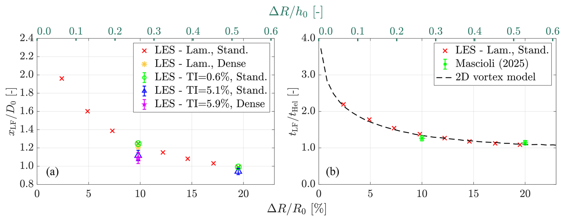
Figure 14 (a) Leapfrogging distance x_LF obtained through the LESs with different ΔR, inflow conditions, and mesh resolutions. (b) Leapfrogging time t_LF predicted by the 2D vortex model and LESs subjected to laminar inflow conditions with the standard mesh together with the experimental results of Mascioli (2025).

Similar to σ_LES, both inflow turbulence intensity TI and mesh resolution are found to have minimal effects on the leapfrogging distance x_LF. Particularly focusing on when TI differs, the leapfrogging distances when TI=0.6 % (green circles in Fig. 14a) are very close to those obtained with laminar inflow conditions, while when TI=5.1 % (blue triangles in Fig. 14a), the data become more scattered, with mean values of x_LF being less than 6 % lower than those subjected to laminar conditions. To conclude, the minimal deviation in x_LF and σ_LES between laminar and turbulent inflow conditions suggests that inflow turbulence has minor effects on the near-wake tip vortex behavior for the asymmetric rotor studied in this work, particularly regarding the leapfrogging phenomenon. However, it should be noted that inflow turbulence still plays an important role in triggering secondary instabilities of the vortex helix, as widely reported in the literature (Ivanell et al., 2010; Wang et al., 2022; Hodgkin et al., 2023), and this can also be identified in the animations provided in the accompanied data repository (Yen et al., 2025).

Figure 14b plotted the leapfrogging time t_LF obtained through different methods against ΔR. The results from the 2D vortex model show good agreement with the LESs under laminar inflow conditions, with elative deviations of no more than 7 % across the range of ΔR considered. A similar level of agreement has also been reported in Abraham et al. (2023a). Furthermore, analogous to the behavior of x_LF, the value of t_LF approaches an asymptotic value as ΔR surpasses 0.5h₀. This asymptotic value corresponds to $\mathrm{\Gamma }/\mathrm{2}{h}_{\mathrm{0}}^{\mathrm{2}}$, which can be explained by Eq. (8), where $\mathrm{d}\mathit{\delta }h/\mathrm{d}t$ approaches with a velocity of $\mathrm{\Gamma }/\mathrm{2}{h}_{\mathrm{0}}$ as δr≫h₀. Dividing h₀ by this velocity yields $\mathrm{2}{h}_{\mathrm{0}}^{\mathrm{2}}/\mathrm{\Gamma }$, which is the time needed to complete the first leapfrogging event. This relationship was previously highlighted by Quaranta et al. (2015) and forms the basis for using $t_{\text{Hel}}\equiv \mathrm{2}{h}_{\mathrm{0}}^{\mathrm{2}}/\mathrm{\Gamma }$ as the characteristic timescale in this study. As shown in Fig. 14b, t_Hel indeed serves as the asymptotic value for t_LF as ΔR increases for both the LESs and the 2D vortex model. This agreement further demonstrates that the methodologies and analysis techniques employed in the current work are well-grounded in established theoretical frameworks.

In addition to the numerical results and theoretical predictions, two data points from wind tunnel experiments (Mascioli, 2025) are also provided for comparison in Fig. 14b. The experiments were conducted in the low-speed wind tunnel at Delft University of Technology (W-tunnel), which was configured as an open jet with a cross-sectional area of 60 cm×60 cm at the outlet. The tested inflow velocity was approximately 5.4 ms⁻¹, with a turbulence intensity below 2 %. Particle image velocimetry (PIV) was employed to capture the flow field. The rotor model used in the experiments was a four-bladed configuration with a diameter of 30 cm, operating at a tip speed ratio of 3.5. This setup results in a helix geometry comparable to that of the LESs, with both configurations featuring $h_{\mathrm{0}}/D_{\mathrm{0}}\simeq \mathrm{0.2}$. The trajectories of the tip vortices in the experiments were tracked using the same method applied to the LESs (see Sect. 3.2.1). The measured circulation strength of the tip vortices in the experiments was approximately 0.08 m² s⁻¹.

As shown in Fig. 14b, the experimental data align remarkably well with the predictions of the 2D vortex model and the results of the LESs, despite the Reynolds numbers based on the diameter ($U_{\mathrm{\infty }}{D}_{\mathrm{0}}/\mathit{\nu }$) and the circulation ($\mathrm{\Gamma }/\mathit{\nu }$) being several orders different. This strong consistency between the theoretical predictions, numerical results, and experimental measurements further reinforces the validity of the findings of the present study.

3.3 Streamwise evolution of the wake quantities

While the study of vortex dynamics provides valuable insights into the leapfrogging instability, the wake velocity is of greater practical importance for wind turbine and wind farm performance. In particular, the streamwise evolution of the wake velocity is a key parameter for evaluating wake recovery. Therefore, in addition to vorticity fields, special attention is given to the mean velocity profiles, $\stackrel{\mathrm{‾}}{u}$, across cases with varying rotor asymmetries, inflow conditions, and mesh resolutions. The temporal statistics used to compute these profiles are collected over sufficiently long periods to ensure statistical convergence, particularly five rotor revolutions for laminar inflow cases and 100 rotor revolutions for turbulent inflow cases.

In this subsection, for the sake of brevity, only the cases with a symmetric rotor and those with $\mathrm{\Delta }R/R_{\mathrm{0}}\simeq \mathrm{10}\mathrm{\%}$ are considered. Cases with other levels of asymmetry exhibit very similar behavior and are therefore not presented and discussed in detail.

3.3.1 Contours of streamwise mean velocity $\stackrel{\mathrm{‾}}{u}$

Downstream of a symmetric rotor subjected to laminar inflow conditions (Fig. 15a), a clear region of significant velocity deficit, known as the wake, is observed. After wake expansion ceases around $x/D_{\mathrm{0}}=\mathrm{1}$, the shear layer remains stable further downstream, consistent with the ω_y fields shown in Fig. 5a, where undisturbed tip vortices form a stable vortex tube. This observation aligns well with the findings of Troldborg (2009) and Li et al. (2024). When a blade length difference of $\mathrm{\Delta }R/R_{\mathrm{0}}\simeq \mathrm{10}\mathrm{\%}$ is introduced (Fig. 15b), the overall characteristics of the $\stackrel{\mathrm{‾}}{u}$ field remain similar to those of the symmetric rotor case, suggesting that the wake recovery rate is not significantly affected by this level of rotor asymmetry.

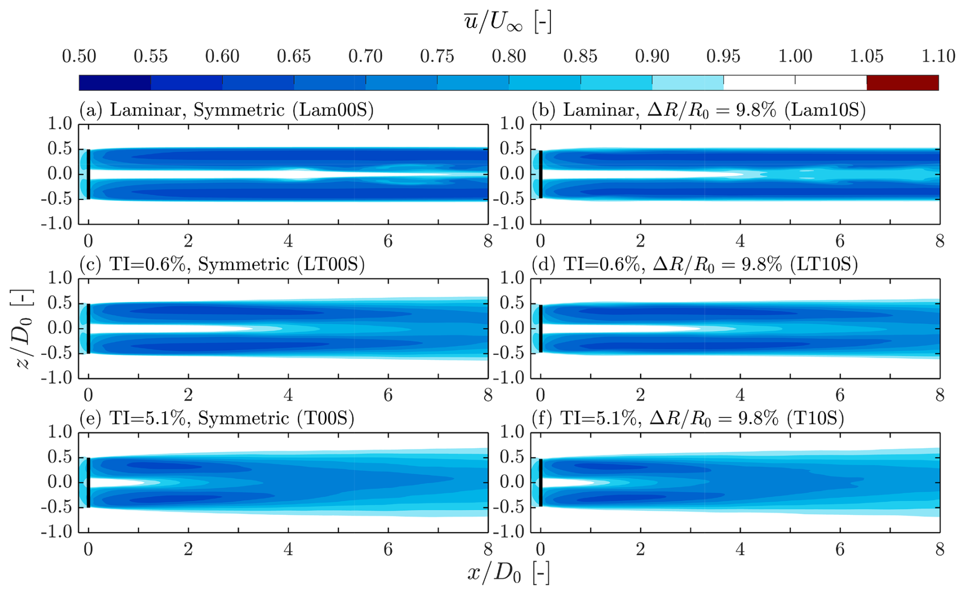
Figure 15 Contours of the mean streamwise velocity $\stackrel{\mathrm{‾}}{u}$ for cases with the standard mesh subjected to laminar inflow conditions, TI=0.6 %, and TI=5.1 % and blade length differences of $\mathrm{\Delta }R/R_{\mathrm{0}}\simeq [\mathrm{0}\mathrm{\%},\mathrm{10}\mathrm{\%}]$. The corresponding TI and ΔR values, together with their case names (see Table 1), are labeled at the top left of each panel. The black lines indicate the position of the rotor.

For cases subjected to TI=0.6 %, the shear layer exhibits continuous downstream spreading for both symmetric and asymmetric rotors, as shown in Fig. 15c and d. When the turbulence intensity increases to TI=5.1 %, the spreading becomes even more pronounced, as observed in Fig. 15e and f. Overall, it is evident that the extent of the wake deficit is more strongly influenced by TI than by ΔR. In particular, higher turbulence intensity leads to more rapid shear layer spreading, while the impact of rotor asymmetry remains minimal. As illustrated in Fig. 6, ambient turbulence disrupts the tip vortex helices, which typically act to suppress wake breakdown (Medici, 2005). The breakdown of these vortex helices enhances momentum exchange between the wake and the surrounding flow, promoting lateral spreading of the velocity deficit and reducing the peak momentum deficit along the wake centerline.

3.3.2 Line plots of streamwise mean velocity $\stackrel{\mathrm{‾}}{u}$ at selected streamwise positions

To further investigate the recovery of momentum deficit, velocity profiles at $x/D_{\mathrm{e}}=\mathrm{2}$, 5, and 8 downstream are presented in Fig. 16, where D_e denotes the effective diameter (see Table 1).

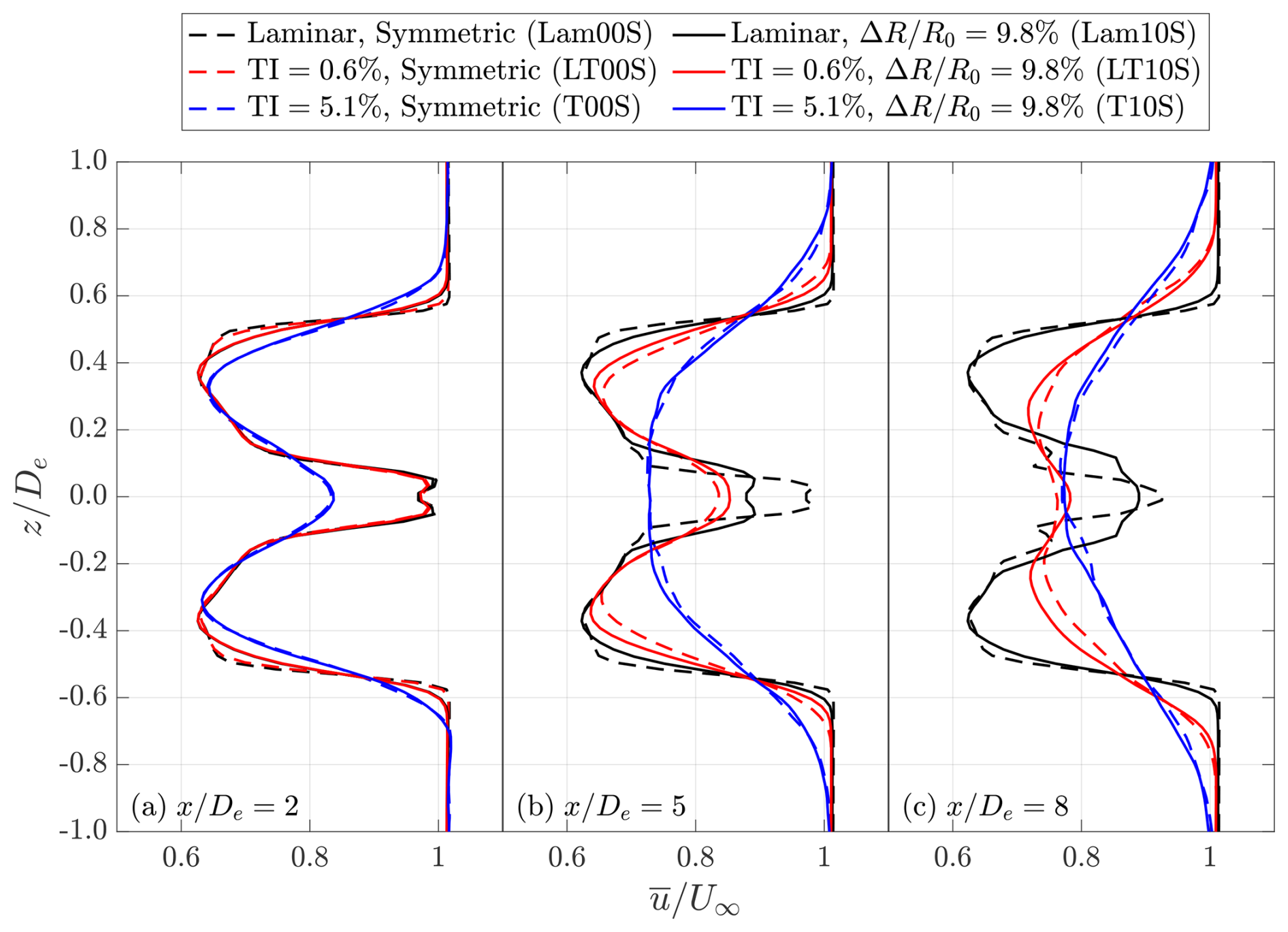
Figure 16 Streamwise velocity profiles sampled at 2D_e, 5D_e, and 8D_e for cases with $\mathrm{\Delta }R/R_{\mathrm{0}}\simeq [\mathrm{0}\mathrm{\%},\mathrm{10}\mathrm{\%}]$ under different inflow conditions. The case names are introduced in Table 1.

At $x/D_{\mathrm{e}}=\mathrm{2}$ (Fig. 16a), all cases exhibit the characteristic near-wake velocity profile of a wind turbine, with a pronounced velocity deficit around 0.65U_∞ at the center and higher velocities near the hub region. Strong velocity shear is present in both the tip and hub regions, indicated by sharp velocity gradients. Under laminar inflow conditions (black lines) and at TI=0.5 % (red lines), the velocity profiles show intricate but noticeable sensitivity to rotor asymmetry, with stronger shear at the tips for the symmetric rotor. This is attributed to periodic loading variations near the tip caused by blade length differences, which reduce the sharpness of the time-averaged loading gradient in those asymmetric cases. However, as the turbulence intensity increases to TI=5.1 % (blue lines), the influence of rotor asymmetry becomes unidentifiable. For both the wakes of a symmetric and an asymmetric rotor, the velocity gradients become more gentle, and the velocity deficits become milder with stronger ambient turbulence, indicating enhanced momentum diffusion and accelerated wake recovery.

As the flow progresses from $x/D_{\mathrm{e}}=\mathrm{2}$ to 5 and then to 8, the spatial evolution of the wake can be further examined through the velocity profiles.

When subjected to laminar inflow conditions, noticeable changes when moving downstream primarily occur near the hub region for both symmetric and asymmetric rotors, where the initially sharp velocity gradients gradually smooth out with increasing downstream distance. However, the overall structure of the wake remains largely unchanged, as clearly demonstrated by the velocity contour plots in Fig. 15a and b, which show minimal wake development and recovery under laminar inflow conditions.

When TI=0.5 %, the wake progressively evolves toward the well-known self-similar profiles described in the literature (Porté-Agel et al., 2011), as clearly observed in the $\stackrel{\mathrm{‾}}{u}$ profiles at $x/D_{\mathrm{e}}=\mathrm{5}$ and $x/D_{\mathrm{e}}=\mathrm{8}$. The concave velocity deficit near mid-span flattened due to enhanced turbulent mixing, with the symmetric rotor case showing slightly more advanced development. At TI=5.1 %, the effects of turbulent mixing become even more pronounced. The inflection points in the velocity profiles vanish as early as $x/D_{\mathrm{e}}=\mathrm{5}$, and the velocity deficit spreads further outward in the radial direction, indicating a stronger mixing process and accelerated wake recovery.

3.3.3 Area-averaged streamwise mean velocity $\langle \stackrel{\mathrm{‾}}{u}{\rangle }_{\text{disk}}$

In this study, the disk-averaged mean streamwise velocity, $\langle \stackrel{\mathrm{‾}}{u}{\rangle }_{\text{disk}}$, is employed as an integral metric to evaluate wake recovery. It is calculated by averaging the mean streamwise velocity, $\stackrel{\mathrm{‾}}{u}$, over a circular disk with an effective diameter D_e. This metric provides an integrated measure of the overall streamwise velocity and serves as an estimator for the wind resource available to a downstream turbine. A more rapid increase in $\langle \stackrel{\mathrm{‾}}{u}{\rangle }_{\text{disk}}$ along the streamwise direction can be interpreted as stronger and faster wake recovery.

Figure 17 presents the evolution of $\langle \stackrel{\mathrm{‾}}{u}{\rangle }_{\text{disk}}$ at various downstream locations for cases with different rotor asymmetries, inflow turbulence intensities, and mesh resolutions. It is important to note that the characteristic length scale used is the effective diameter, D_e, which varies slightly between cases depending on rotor asymmetry (see Table 1). For all cases, $\langle \stackrel{\mathrm{‾}}{u}{\rangle }_{\text{disk}}$ initially drops to approximately 0.7U_∞ just behind the rotor, reflecting the energy extraction by the turbine. Under laminar inflow conditions, little to no increase in $\langle \stackrel{\mathrm{‾}}{u}{\rangle }_{\text{disk}}$ is observed for both symmetric and asymmetric rotors, indicating limited momentum recovery. When low-level inflow turbulence (TI=0.6 %) is introduced, noticeable recovery is evident. At TI≃5 %, the increase in $\langle \stackrel{\mathrm{‾}}{u}{\rangle }_{\text{disk}}$ becomes even more pronounced. However, across all turbulence levels, no significant differences are observed between symmetric and asymmetric rotors, suggesting that rotor asymmetry has minimal influence on wake recovery in the presence of turbulence.

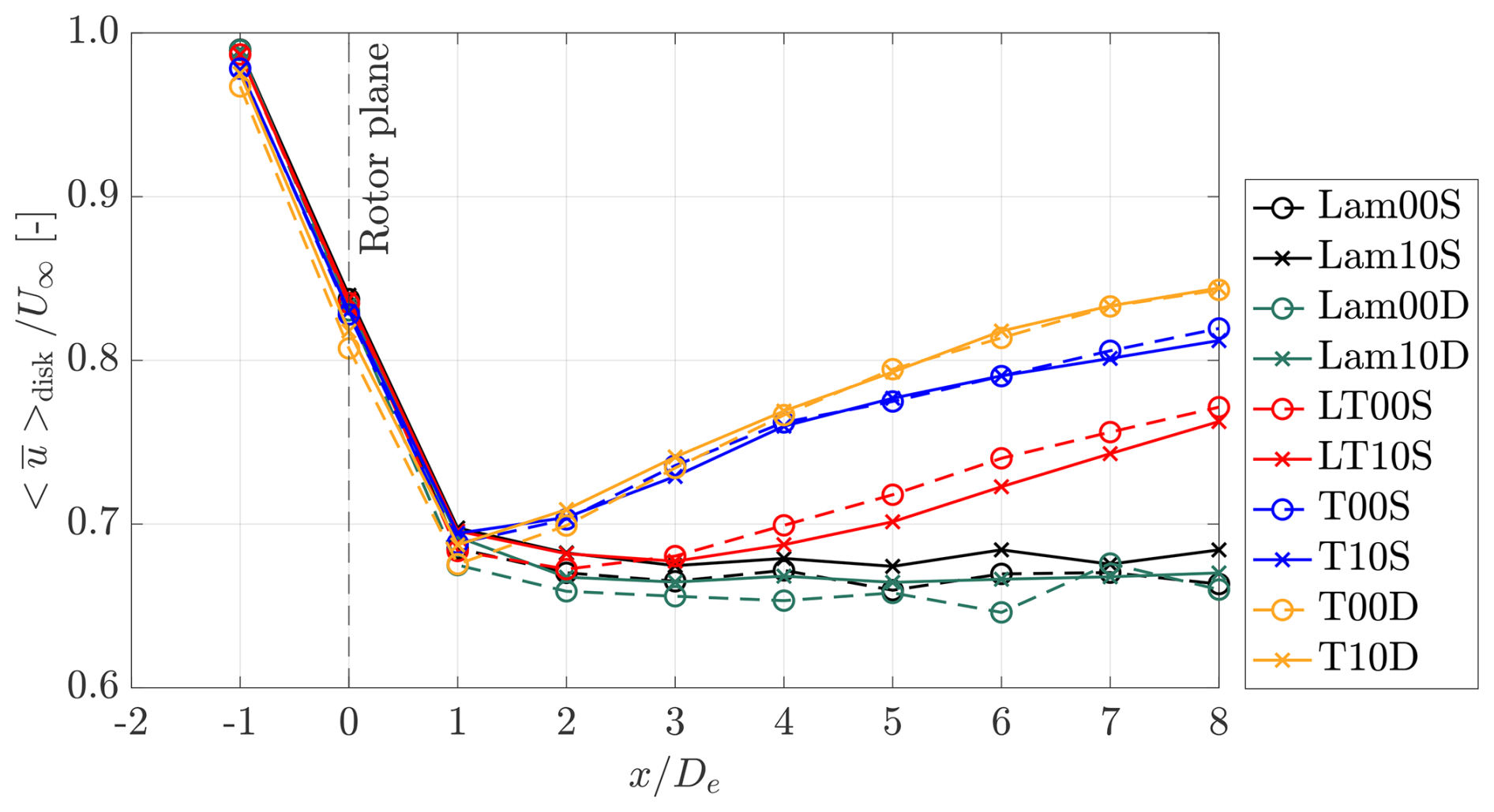
Figure 17 Disk-averaged mean streamwise velocity $\langle \stackrel{\mathrm{‾}}{u}{\rangle }_{\text{disk}}$ for the cases with different rotor asymmetries, subjected to various inflow conditions, and simulated with both standard and dense mesh resolutions. The case names are introduced in Table 1.

The trend observed in $\langle \stackrel{\mathrm{‾}}{u}{\rangle }_{\text{disk}}$ is predominantly influenced by the turbulence intensity (TI) rather than rotor asymmetry. As TI increases, the velocity recovers more rapidly, indicating more effective wake recovery. This observation is consistent with previous studies in the literature (Li et al., 2016; Talavera and Shu, 2017; Angelou et al., 2023). When these findings are combined with observations with the ω_y contours (Figs. 5 and 6) and phase-averaged vorticity magnitude fields $\stackrel{\mathrm{̃}}{\left|{\mathit{\omega }}_y\right|}$ (Fig. 7), a clear relationship emerges between the leapfrogging and the wake recovery process. Specifically, the rotor asymmetries considered in this study trigger the leapfrogging phenomenon but do not promote wake breakdown. Instead, new stable helices formed from paired tip vortices are established in the wake of an asymmetric rotor, resembling the helical structures seen in symmetric rotor cases. These stable structures (structures in equilibrium, to be precise) again delay mixing between the wake and the surrounding freestream. As a result, with the absence of vortex breakdown, which can be induced by ambient turbulence or other mechanisms, the wake recovery rate is not significantly enhanced by rotor asymmetries alone.

The findings presented in this study appear to contrast with those reported by Lignarolo et al. (2015), who conducted experiments using a two-bladed wind turbine rotor with uneven blade pitch angles to trigger leapfrogging. In their work, they concluded that leapfrogging accelerates wake recovery by promoting wake breakdown. However, the cases with laminar inflow presented in this study indicate that leapfrogging alone does not necessarily accelerate wake recovery, which is supported by the profiles of $\langle \stackrel{\mathrm{‾}}{u}{\rangle }_{\text{disk}}$ (Fig. 17) and the vorticity contours (Fig. 5). This discrepancy can likely be attributed to the presence of other secondary instabilities in the experiments conducted by Lignarolo et al. (2015), such as the local vortex pairing observed by Quaranta et al. (2019). These secondary instabilities can arise from unavoidable experimental perturbations, including structural vibrations, turbulence originating from blade boundary layers, and rotor imperfections. As these instabilities develop, they disrupt the coherence and symmetry of the tip vortex helices, potentially serving as the primary drivers of wake breakdown (Hodgkin et al., 2023). Therefore, the sudden momentum ingestion observed by Lignarolo et al. (2015) may not be entirely attributed to leapfrogging but may instead be only correlated with it. This interpretation is further supported by the current simulation results. When under laminar inflow conditions, $\langle \stackrel{\mathrm{‾}}{u}{\rangle }_{\text{disk}}$ in Fig. 17 remains relatively constant, while in cases with TI=0.6 %, it begins to increase after x_LF. Therefore, combining this observation and the vorticity contours provided in Figs. 5 and 6, it can be concluded that the driver of the wake breakdown process is turbulence-induced instabilities, rather than leapfrogging alone.

The present findings also diverge from those of Abraham et al. (2023b), who, using vortex modeling, reported an 11 % increase in available power (area-averaged ${\stackrel{\mathrm{‾}}{u}}^{\mathrm{3}}$ over an area of $\mathit{\pi }{R}_{\mathrm{0}}^{\mathrm{2}}$) for an asymmetric rotor ($\mathrm{\Delta }R/R_{\mathrm{0}}\simeq \mathrm{2}\mathrm{\%}$) compared to a symmetric rotor at a downstream distance of 7D₀ when subjected to laminar inflow conditions. Several factors are likely to contribute to this discrepancy. Notably, their study employs a three-bladed rotor and includes the floor in the simulation setup, whereas the current work uses a two-bladed rotor and excludes the floor. These differences are known to influence the vortex dynamics in wind turbine wakes, as they affect rotor loading, the pitch between successive tip vortices (i.e., the equivalent h₀), and the overall symmetry of the system (Troldborg, 2009; Ramos-García et al., 2023). Additionally, the numerical frameworks used in the two studies differ substantially. It is worth noting that both the LES approach with actuator lines used in the present study and the vortex model with lifting lines employed in their work are relatively sensitive to the choice of model parameters (Martínez-Tossas et al., 2015; Branlard, 2017). These include spatial and temporal discretization, vortex core treatment, and diffusion modeling. All of the factors discussed in this paragraph may each partially contribute to the differences in the reported outcomes, and a precise identification of their individual effects is left for future work.

4 Sensitivity tests on the selected parameters

To further validate the numerical methods employed in this study, several key parameters commonly considered in LES with ALM for similar applications are examined in this section. These aspects include the vortex core radius r_ω, the blockage ratio (rotor area relative to the cross-sectional area of the computational domain), and the diffusivity. To assess how these parameters are influenced by simulation settings and to evaluate their impact on the results and conclusions, several supplementary simulations have been performed and compared with the representative cases listed in Table 1. These additional cases are summarized in Table 3. For brevity, all these supplementary cases feature an asymmetric rotor with $\mathrm{\Delta }R/R_{\mathrm{0}}\simeq \mathrm{10}\mathrm{\%}$ and are subjected to laminar inflow conditions. Aside from the specified parameters, all other simulation settings match those of cases Lam10S and Lam10D in Table 1. Note that the mesh configurations for dense cases are detailed in Sect. 2.4.4.

Table 3 Supplementary cases for the parametric study. All cases listed in this table have an asymmetric rotor with $\mathrm{\Delta }R/R_{\mathrm{0}}\simeq \mathrm{10}\mathrm{\%}$ and are subjected to laminar inflow conditions. The columns from left to right document the case names, mesh resolution, thrust coefficient, power coefficient, normalized growth rate, normalized leapfrogging time, and remarks for each case. Note that the cases with asterisks have already been introduced in Table 1 and that the suffix behind the underscore sign corresponds to the remarks.

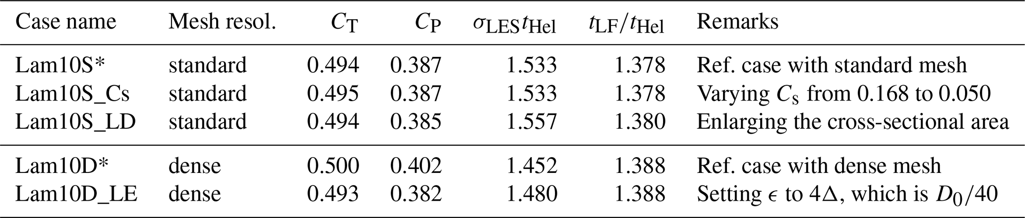
The vortex core radius r_ω is expected to be primarily influenced by the absolute size of the smoothing factor ϵ in Eq. (4), which is typically closely coupled to the grid size Δ. To assess the impact of r_ω, both ϵ and Δ are varied, with comparisons drawn between cases Lam10S, Lam10D, and Lam10D_LE. Regarding the blockage ratio, an additional simulation with an enlarged computational domain of 10D₀×10D₀ (case Lam10S_LD) is conducted. This domain size is compared four times to that of the reference cases (5D₀×5D₀, Lam10S), reducing the blockage ratio from 3.1 % to 0.7 %. Finally, regarding diffusivity, it is tested by varying the parameters related to the turbulence model, the grid size, and the numerical scheme employed.

4.1 Vortex core size

Following the previous studies on leapfrogging instability (Quaranta et al., 2015; Ramos-García et al., 2023), the core size of the helical vortices, r_ω, is defined as the radial distance from the vortex centroid at which the tangential velocity u_ϕ reaches its maximum. In line with the approach used to determine Γ and h₀ in Sect. 3.2.2, the analysis in this subsection focuses on vortices shed from the un-truncated blade, evaluated when their vortex age corresponds to half a rotor rotation period (torsional effects are not corrected). Note that the difference in r_ω between the truncated and the un-truncated blades can be determined with the data in Table 3. Figure 18 presents the profiles of u_ϕ as a function of the radial distance r for the five cases listed in Table 3, with the corresponding r_ω values indicated. The results show that r_ω is not influenced by the domain size or the value of C_s. On the other hand, by comparing cases Lam10D and Lam10D_LE with case Lam10S, it is evident that r_ω is more sensitive to the absolute value of the smoothing factor ϵ than to the mesh resolution. Specifically, ϵ is set to $D_{\mathrm{0}}/\mathrm{80}$ for case Lam10D and to $D_{\mathrm{0}}/\mathrm{40}$ for all the other four cases in Table 3. Note that the ratio $\mathit{ϵ}/\mathrm{\Delta }$ is set to 4 for case Lam10D_LE, whereas all other cases use a ratio of 2.

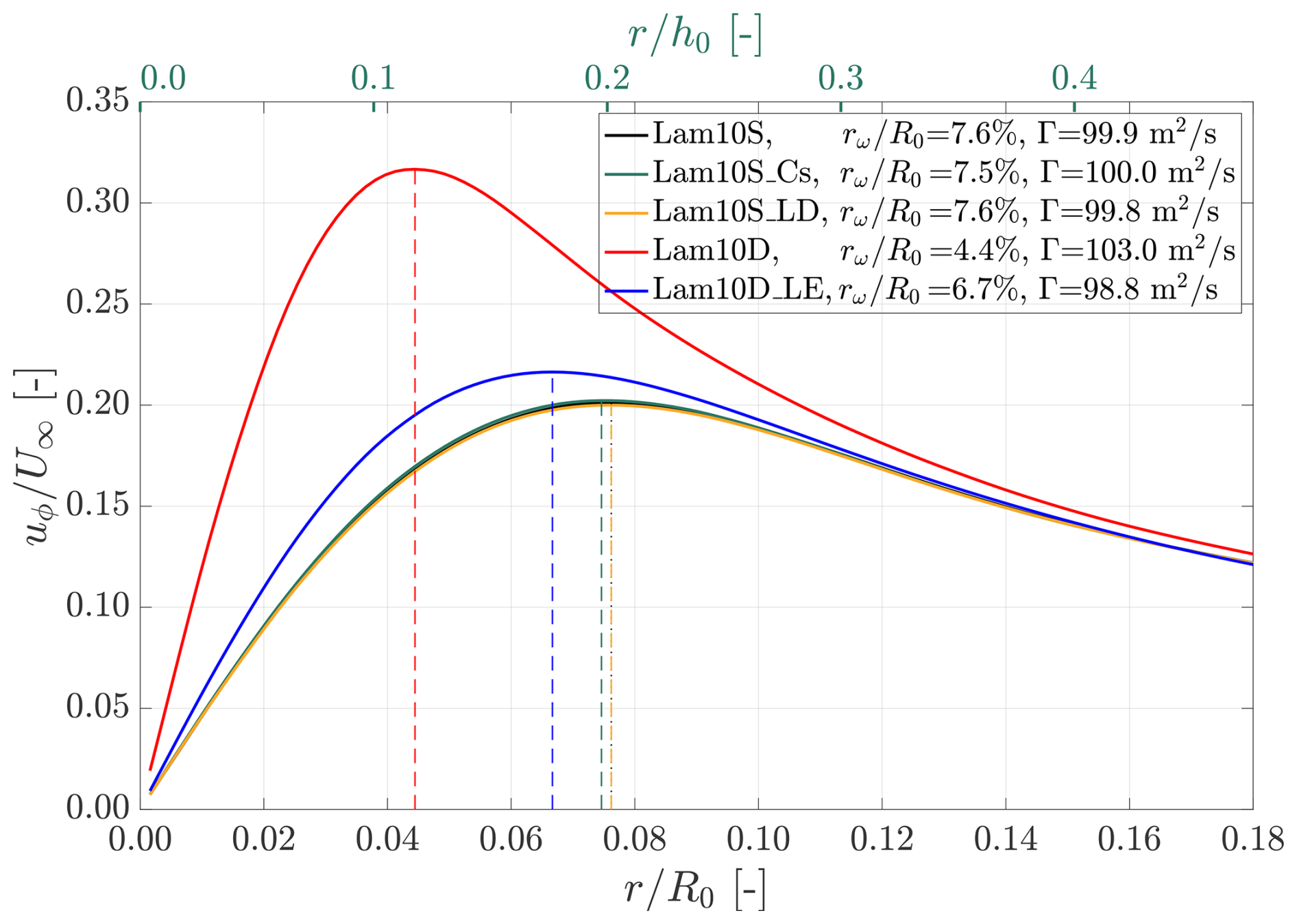
Figure 18 Profiles of the tangential velocity around the vortex centroid, u_ϕ, plotted against the radial distance from the vortex centroid, r, for the five cases listed in Table 3. The radial positions corresponding to the maximum u_ϕ for each case are indicated by vertical dashed lines, representing the vortex core size r_ω. The exact values of r_ω and Γ are provided in the figure legend.

According to theoretical predictions (Martínez-Tossas and Meneveau, 2019), the minimum vortex core radius r_ω that can be resolved using the current numerical setup (LES with ALM) is approximately 1.12ϵ. In particular, when ϵ=2Δ is applied, the cases with the standard mesh (Lam10S) and the dense mesh (Lam10D) of this study can theoretically resolve r_ω down to $\mathrm{5.6}\times {\mathrm{10}}^{-\mathrm{2}}{R}_{\mathrm{0}}$ and $\mathrm{2.8}\times {\mathrm{10}}^{-\mathrm{2}}{R}_{\mathrm{0}}$, respectively. These theoretical limits are fairly close to the r_ω values obtained from the simulations, namely, $\mathrm{7.6}\times {\mathrm{10}}^{-\mathrm{2}}{R}_{\mathrm{0}}$ for case Lam10S and $\mathrm{4.4}\times {\mathrm{10}}^{-\mathrm{2}}{R}_{\mathrm{0}}$ for case Lam10D. This agreement reinforces that ϵ is the primary parameter controlling r_ω. Additionally, the slightly larger r_ω observed in the LES results compared to the theoretical limits is primarily due to the gradual reduction of blade loading near the tip, rather than an abrupt cutoff.

In the work of Selçuk et al. (2017), it was shown that the detailed dynamics of helical vortices are strongly influenced by the ratio $r_{\mathit{\omega }}/h_{\mathrm{0}}$. Their study demonstrated that the onset of vortex merging begins when $r_{\mathit{\omega }}/h_{\mathrm{0}}\ge \mathrm{0.12}$ for cases where ΔR≪h₀. The results of the present work align closely with these findings. Specifically, for the case with $\mathit{ϵ}=D_{\mathrm{0}}/\mathrm{40}$ (Lam10S), vortex merging begins immediately during the first leapfrogging event, with $r_{\mathit{\omega }}/h_{\mathrm{0}}$ measured at 0.20 for newly shed vortices (those enclosed by the circles in Fig. 10). In contrast, for the case with $\mathit{ϵ}=D_{\mathrm{0}}/\mathrm{80}$ (Lam10D), merging occurs much later. It happens after the second leapfrogging event, and $r_{\mathit{\omega }}/h_{\mathrm{0}}$ is found to be 0.11 in the immediate vicinity of the rotor.

To illustrate the impact of vortex core size more clearly, vorticity contours of ω_y for the relevant cases are presented in Fig. 19. In general, the positions of the vortex centroids remain nearly identical across all cases listed in Table 4 up to $x/D_{\mathrm{0}}<\mathrm{1.5}$, after which vortices in cases with $\mathit{ϵ}=D_{\mathrm{0}}/\mathrm{40}$ begin to merge. This observation indicates that, prior to the onset of merging, the motion of vortex centroids is not significantly influenced by r_ω, consistent with the findings of Selçuk et al. (2017). This further suggests that the dynamics of vortex centroids, and thus the leapfrogging instability, are predominantly governed by inviscid processes before vortex merging occurs.

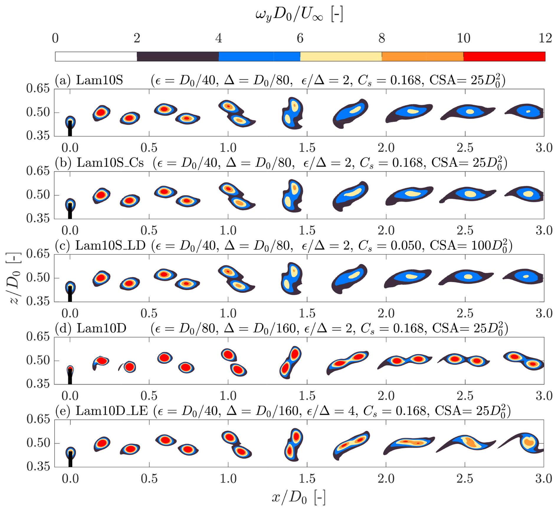
Figure 19 Contours of out-of-plane vorticity ω_y for the five cases listed in Table 3, with the fields shown around the tip height. Case names and the parameters of interest are indicated at the top of each panel. CSA is the abbreviation for the cross-sectional area of the computational domain.

In addition to the similarities in the positions of the vortex centroids, it can be observed that the case with $\mathit{ϵ}=D_{\mathrm{0}}/\mathrm{80}$ (Lam10D) exhibits smaller and more concentrated vortices compared to the cases with $\mathit{ϵ}=D_{\mathrm{0}}/\mathrm{40}$ (the other four cases), which is consistent with the results shown in Fig. 18. Moreover, for cases with the same value of ϵ but different grid sizes Δ (e.g., Lam10S and Lam10D_LE, both with $\mathit{ϵ}=D_{\mathrm{0}}/\mathrm{40}$ but different Δ), the vorticity contours show greater similarity compared to cases with the same Δ but different ϵ (e.g., Lam10D and Lam10D_LE, both with $\mathrm{\Delta }=D_{\mathrm{0}}/\mathrm{160}$ but different ϵ). This again clearly demonstrates that the vortex core size r_ω is primarily determined by the choice of ϵ.

4.2 Cross-sectional blockage ratio

The impact of the cross-sectional blockage ratio is primarily evaluated by comparing the rotor performance metrics. It is anticipated that the effects of the blockage ratio will be reflected in the rotor performance metrics, with excessive blockage leading to overestimations of C_T and C_P (Sarlak et al., 2016). As shown in Table 4, reducing the blockage ratio from 3.1 % to 0.7 % results in changes to the rotor performance of less than 0.5 %, indicating that a blockage ratio of 3.1 % is not excessive. Furthermore, both σ_LES and t_LF remain unaffected by the domain size, further confirming that the cross-sectional size used in the current numerical setup is sufficient. The ω_y contours in Fig. 19 also demonstrate that the cross-sectional area has virtually no impact on the vortex dynamics by comparing the contour of case Lam10S_LD with that of Lam10S.

4.3 Diffusivity

The vortex core size r_ω increases over time due to diffusivity effects (Cerretelli and Williamson, 2003), with faster growth observed under stronger diffusivity. In the current setups, one of the key parameters influencing diffusivity is the modeled eddy viscosity ν_sgs, which depends on the Smagorinsky constant C_s and the grid size Δ, as described in Eq. (2). To assess the impact of diffusivity, cases Lam10S, Lam10S_Cs (where C_s is reduced from 0.168 to 0.050), and Lam10D_LE are compared, as they differ in C_s and Δ but share the same values for other key parameters (e.g., $\mathit{ϵ}=D_{\mathrm{0}}/\mathrm{40}$). Overall, for the considered cases, the effects of diffusivity are found to be minimal, as indicated by the vorticity contours in Fig. 19. Additionally, the values of σ_LES and t_LF in Table 4 further confirm that diffusivity has negligible influence on leapfrogging-related quantities.

In Fig. 19, it can be observed that the maximum vorticity within the vortex cores is better preserved with smaller values of C_s and finer grid resolution Δ when comparing cases Lam10S_Cs and Lam10D_LE with Lam10S, as expected. Additionally, the influence of varying Δ appears more significant than that of varying C_s. This is likely due to the effects of numerical dissipation (see Appendix A), which become more pronounced with larger Δ (Ferziger et al., 2002). However, further quantification of those effects is not pursued, as the impacts of diffusivity are found to be minor within the current setup and are thus considered beyond the scope of this study.

4.4 Remarks

With the detailed parametric study conducted, it can be stated with confidence that the leapfrogging-instability-related quantities obtained in this study are robust against the variations of the surveyed parameters. Throughout this investigation, it has been demonstrated that both the vortex core size r_ω and diffusivity have negligible impact on the leapfrogging growth rate. Furthermore, the vortex dynamics leading up to the first leapfrogging event are not significantly influenced by r_ω or diffusivity within the explored parameter space. An important practical conclusion is that the resolution of the standard mesh is sufficient if the detailed vortex behavior beyond the first leapfrogging event is not the focus. This remark is of particular importance, as high-fidelity simulations are often limited by available computational resources. Knowing that the key physics of interest can be accurately captured using much less computationally demanding setups can greatly facilitate future research efforts. This enables more efficient use of computational resources and allows for broader parametric studies to be done within some practical budget constraints.

5 Conclusions and recommendations

The near-wake behavior of a two-bladed utility-scale wind turbine rotor with varying degrees of asymmetry was investigated using large-eddy simulations combined with the actuator line model. The rotor model employed was a modified version of the NREL 5 MW baseline turbine, with rotor asymmetry introduced by varying the blade length difference from 0 % to 30 %. The numerical results were further consolidated through comparisons with theoretical predictions using a two-dimensional point vortex model and supported by experimental measurements. Additionally, the simulation settings for the selected cases were provided in the accompanying data repository (Yen et al., 2025), with the aim of supporting and facilitating future research efforts in this area.

The leapfrogging instability growth rate obtained from the LES results was found to decrease with increasing blade length difference, in agreement with the predictions of the 2D vortex model. Furthermore, the leapfrogging time derived from the LES data showed good agreement with both the 2D vortex model and wind tunnel experiments (Mascioli, 2025), confirming that rotor asymmetry accelerated the onset of leapfrogging. When increasing the asymmetry, the apparent contradiction between the decreasing growth rate and the earlier onset of leapfrogging was primarily attributed to differences in initial conditions that influence the early dynamics of the vortex pairs.

Despite the studied rotor asymmetries triggering an earlier onset of leapfrogging, their contributions to accelerating the large-scale breakdown of the helical vortex system and the subsequent wake recovery were found to be minimal. This result contrasted with the findings of Abraham et al. (2023b), where they found an accelerated wake recovery. Instead, following the leapfrogging event, the vortex system of this work transitioned into a new equilibrium state, indicating that additional mechanisms, such as turbulent fluctuations or structural vibrations, may be needed to initiate wake breakdown and enhance mixing in order to result in a faster wake recovery rate.

Additionally, the inflow conditions were found to have minor effects on the near-wake tip vortex dynamics of an asymmetric rotor, as both the leapfrogging distance and growth rate remained relatively unchanged compared to those observed under laminar inflow conditions. However, inflow turbulence played a dominant role in the wake recovery process, overshadowing the influence of rotor asymmetry even at turbulence levels as low as those found in controlled laboratory environments. Specifically, for the current setups, turbulent fluctuations consistently promoted the wake breakdown process to a similar extent across different levels of rotor asymmetry, highlighting that ambient turbulence, rather than the induced perturbations by the rotor asymmetry, governed the global wake evolution and recovery.

Finally, detailed parametric studies were conducted to verify the reliability of the current numerical setup. The effects of vortex core size and flow diffusivity on the tip vortex dynamics of the asymmetric rotor were examined by varying the mesh resolution, actuator line model parameters (smoothing factor ϵ), and turbulence model parameters (Smagorinsky constant C_s). The results demonstrated that with the exception of the detailed vortex behavior beyond the first leapfrogging event, such as vortex merging, the key leapfrogging-related quantities remained largely unaffected within the tested parameter range. This confirmed that the numerical framework employed in this study was robust and sufficient for capturing the primary dynamics of the leapfrogging instability and near-wake behavior.

In general, this study provided critical insights into the wake aerodynamic behavior of two-bladed asymmetric rotors, particularly regarding their influence on the onset of leapfrogging instability and wake recovery under both laminar and turbulent inflow conditions. By systematically exploring a broad range of rotor asymmetries, it was demonstrated that asymmetry accelerated the onset of leapfrogging when subjected to both laminar and turbulent inflow conditions. However, the results indicated that a shorter leapfrogging distance did not necessarily translate into faster wake recovery. These findings not only addressed existing gaps in the literature concerning the behavior of asymmetric rotors under realistic turbulent inflow conditions but also highlighted the possible limitations of rotor asymmetry as a passive control strategy for enhancing wake recovery.

Several aspects are recommended for future work to further advance the understanding of leapfrogging instability for real-world wind turbines. First, detailed investigations incorporating modal analysis are expected to provide deeper insights, particularly regarding how leapfrogging-related modes interact with the mean flow, stochastic fluctuations, and other instability modes. Such analyses can potentially further clarify the relationship between leapfrogging instability and the wake breakdown process (Biswas and Buxton, 2024b). Furthermore, extending the current study from two-bladed rotors to more commonly used three-bladed rotor configurations is considered an immediate next step. Although recent research has examined three-bladed asymmetric rotors (Abraham and Leweke, 2023; Abraham et al., 2023a, b), those studies remained limited to laminar or very low turbulence inflow conditions. Additionally, examining the role of velocity shear and the presence of the floor on the leapfrogging instability is of critical interest, as these are key characteristics of atmospheric boundary layers but are neglected in the current simulation setups. Finally, field measurements are recognized as an area of great interest, as the ultimate application of wind energy research lies in commercial wind farm operations under realistic atmospheric conditions.

Appendix A: Sensitivity test on the spatial discretization scheme

As mentioned in Sect. 2.4.2, the selection of spatial discretization schemes for the advective term is important because it influences numerical diffusivity as well as numerical stability (Ferziger et al., 2002). To ensure that the numerical scheme employed in this work is proper, a sensitivity test is carried out. The effectiveness of the numerical schemes is briefly surveyed with the contours of the out-of-plane vorticity ω_y in Fig. A1. The setting of interest is the one having $\mathrm{\Delta }R/R_{\mathrm{0}}\simeq \mathrm{10}\mathrm{\%}$, subjected to laminar inflow conditions, and with the standard mesh (case Lam10S in Table 1).

Figure A1 presents the instantaneous ω_y fields obtained using different spatial differencing schemes with the same case setup (Lam10S). Figure A1a illustrates that numerical diffusion is relatively strong when employing the upwind scheme (upwind). In this case, the vortex structures are significantly smeared out, making it difficult to clearly distinguish vortex centroids, and the leapfrogging phenomenon cannot be easily identified. Figure A1b shows the ω_y contours when using the linear upwind scheme (linearUpwind). While this scheme reduces numerical diffusion compared to the pure upwind scheme, allowing the leapfrogging phenomenon to be observed, the vortices remain more diffusive than those obtained with higher-order schemes. Figure A1c presents the results obtained using the second-order central differencing scheme (CDS). Although this approach limits excessive numerical diffusion around the tip and root vortices, it introduces wiggles between the tip vortices, which are attributed to numerical oscillations caused by dispersion errors (Ferziger et al., 2002). Despite these oscillations, the leapfrogging phenomenon can still be captured. Moreover, Fig. A1d shows that the fourth-order CDS exhibits even stronger nonphysical oscillations due to dispersion errors, complicating the analysis of vortex behavior.

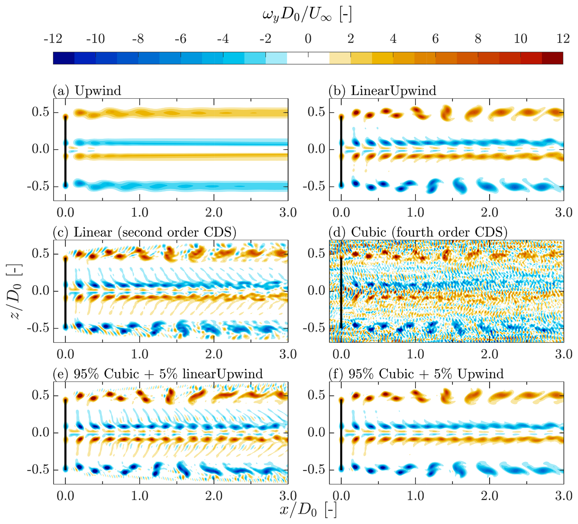
Figure A1 Contours of out-of-plane vorticity ω_y for cases with different numerical schemes for the advective terms ($u_j\partial u_i/\partial x_j$). All the cases follow the setting of Lam10S listed in Table 1, which are all subjected to laminar inflow conditions, have an asymmetric rotor with $\mathrm{\Delta }R/R_{\mathrm{0}}\simeq \mathrm{10}\mathrm{\%}$, and have the standard mesh. Note that CDS is the abbreviation for the central differencing scheme.

In order to achieve results with both high numerical accuracy and minimal numerical oscillations, blended schemes, designed to balance the advantages and drawbacks of different discretization methods (Ivanell et al., 2010; Jha et al., 2014), are tested. Figure A1e shows the results obtained using a blended scheme consisting of 95 % fourth-order CDS and 5 % linear upwind. Although this approach reduces some oscillations, they are still relatively obvious. Figure A1f presents the outcome of using a blended scheme with 95 % fourth-order CDS and 5 % upwind. This formulation produces vortices with minimal numerical diffusion and simultaneously effectively inhibits the numerical dispersion. Compared to the linear upwind scheme (Fig. A1b), the vortices are less diffusive, and the scheme also shows milder oscillations than the previously tested blended approach (Fig. A1e). Therefore, it is concluded that the blended scheme using 95 % fourth-order CDS and 5 % upwind, shown in Fig. A1f, is the most suitable for the present application and is selected for all subsequent simulations.

Appendix B: System linearization

This appendix presents the theoretical prediction of the exponential growth of the leapfrogging instability and provides the justification for using the L₁ norm, $\left|\right|\mathit{\eta }|{|}_{\mathrm{1}}$ (as defined in Eq. 10), to evaluate the growth rates (σ_2D and σ_LES). This analysis is carried out by solving the linearized dynamical system described in Eq. (8), which is repeated in Eq. (B1) for convenience.

$$\begin{array}{ll}{\displaystyle \frac{\mathrm{d}}{\mathrm{d}t}}\left[\begin{array}{c}\mathit{\delta }h\left(t\right)\\ \mathit{\delta }r\left(t\right)\end{array}\right]& {\displaystyle }={\displaystyle \frac{\mathrm{\Gamma }}{\mathrm{2}{h}_{\mathrm{0}}}}\left[\begin{array}{c}\frac{\sinh \left(\mathit{\pi }\mathit{\delta }r/h_{\mathrm{0}}\right)}{\cos \left(\mathit{\pi }\mathit{\delta }h/h_{\mathrm{0}}\right)+\cosh \left(\mathit{\pi }\mathit{\delta }r/h_{\mathrm{0}}\right)}\\ \frac{\sin \left(\mathit{\pi }\mathit{\delta }h/h_{\mathrm{0}}\right)}{\cos \left(\mathit{\pi }\mathit{\delta }h/h_{\mathrm{0}}\right)+\cosh \left(\mathit{\pi }\mathit{\delta }r/h_{\mathrm{0}}\right)}\end{array}\right]\\ \text{(B1)}& {\displaystyle }& {\displaystyle }\equiv {\displaystyle \frac{\mathrm{\Gamma }}{\mathrm{2}{h}_{\mathrm{0}}}}\left[\begin{array}{c}{f}_{\mathit{\delta }h}\left(\mathit{\delta }h\right(t),\mathit{\delta }r(t\left)\right)\\ f_{\mathit{\delta }r}\left(\mathit{\delta }h\right(t),\mathit{\delta }r(t\left)\right)\end{array}\right]\end{array}$$

Starting by letting $\mathit{\delta }h\left(t\right)=\mathit{\delta }{h}_{\mathit{\#}}+\mathit{\delta }{h}^{\prime }\left(t\right)$ and $\mathit{\delta }r=\mathit{\delta }{r}_{\mathit{\#}}+\mathit{\delta }{r}^{\prime }\left(t\right)$, the system equations written in Eq. (B1) at δh=δh_# and δr=δr_# can be linearized to Eq. (B2) when $\mathit{\delta }{h}^{\prime }\ll h_{\mathrm{0}}$ and $\mathit{\delta }{r}^{\prime }\ll h_{\mathrm{0}}$.

$$\begin{array}{ll}{\displaystyle }& {\displaystyle \frac{\mathrm{d}}{\mathrm{d}t}}\left[\begin{array}{c}\mathit{\delta }h\\ \mathit{\delta }r\end{array}\right]={\displaystyle \frac{\mathrm{d}}{\mathrm{d}t}}\left[\begin{array}{c}\mathit{\delta }{h}_{\mathit{\#}}+\mathit{\delta }{h}^{\prime }\left(t\right)\\ \mathit{\delta }{r}_{\mathit{\#}}+\mathit{\delta }{r}^{\prime }\left(t\right)\end{array}\right]={\displaystyle \frac{\mathrm{d}}{\mathrm{d}t}}\left[\begin{array}{c}\mathit{\delta }{h}^{\prime }\\ \mathit{\delta }{r}^{\prime }\end{array}\right]\\ {\displaystyle }& {\displaystyle }\stackrel{\text{Linearization}}{⟶}\underset{\mathbf{J}{|}_{\mathit{\delta }{h}_{\mathit{\#}},\mathit{\delta }{r}_{\mathit{\#}}}}{\underbrace{{\displaystyle \frac{\mathrm{\Gamma }}{\mathrm{2}{h}_{\mathrm{0}}}}\left[\begin{array}{cc}\frac{\partial f_{\mathit{\delta }h}}{\partial \mathit{\delta }h}{|}_{\mathit{\delta }{h}_{\mathit{\#}},\mathit{\delta }{r}_{\mathit{\#}}}& \frac{\partial f_{\mathit{\delta }h}}{\partial \mathit{\delta }r}{|}_{\mathit{\delta }{h}_{\mathit{\#}},\mathit{\delta }{r}_{\mathit{\#}}}\\ \frac{\partial f_{\mathit{\delta }r}}{\partial \mathit{\delta }h}{|}_{\mathit{\delta }{h}_{\mathit{\#}},\mathit{\delta }{r}_{\mathit{\#}}}& \frac{\partial f_{\mathit{\delta }r}}{\partial \mathit{\delta }r}{|}_{\mathit{\delta }{h}_{\mathit{\#}},\mathit{\delta }{r}_{\mathit{\#}}}\end{array}\right]}}\left[\begin{array}{c}\mathit{\delta }{h}^{\prime }\\ \mathit{\delta }{r}^{\prime }\end{array}\right]\\ \text{(B2)}& {\displaystyle }& {\displaystyle }+\underset{\text{forcing terms}}{\underbrace{{\displaystyle \frac{\mathrm{\Gamma }}{\mathrm{2}{h}_{\mathrm{0}}}}\left[\begin{array}{c}{f}_{\mathit{\delta }h}(\mathit{\delta }h=h_{\mathit{\#}},\mathit{\delta }r=r_{\mathit{\#}})\\ f_{\mathit{\delta }r}(\mathit{\delta }h=h_{\mathit{\#}},\mathit{\delta }r=r_{\mathit{\#}})\end{array}\right]}}\end{array}$$

J in Eq. (B2) is the Jacobian matrix of the dynamical system evaluated at (δh_#,δr_#), and its explicit form is given in Eq. (B3).

$$\begin{array}{ll}{\displaystyle }& {\displaystyle }\mathbf{J}={\displaystyle \frac{\mathit{\pi }\mathrm{\Gamma }/\mathrm{2}{h}_{\mathrm{0}}^{\mathrm{2}}}{{\left[\cos \left(\mathit{\pi }\mathit{\delta }{h}_{\mathit{\#}}/h_{\mathrm{0}}\right)+\cosh \left(\mathit{\pi }\mathit{\delta }{r}_{\mathit{\#}}/h_{\mathrm{0}}\right)\right]}^{\mathrm{2}}}}\\ \text{(B3)}& {\displaystyle }& {\displaystyle }\times \left[\begin{array}{cc}\sin \left(\mathit{\pi }\mathit{\delta }{h}_{\mathit{\#}}/h_{\mathrm{0}}\right)\sinh \left(\mathit{\pi }\mathit{\delta }{r}_{\mathit{\#}}/h_{\mathrm{0}}\right)& \mathrm{1}+\cos \left(\mathit{\pi }\mathit{\delta }{h}_{\mathit{\#}}/h_{\mathrm{0}}\right)\cosh \left(\mathit{\pi }\mathit{\delta }{r}_{\mathit{\#}}/h_{\mathrm{0}}\right)\\ \mathrm{1}+\cos \left(\mathit{\pi }\mathit{\delta }{h}_{\mathit{\#}}/h_{\mathrm{0}}\right)\cosh \left(\mathit{\pi }\mathit{\delta }{r}_{\mathit{\#}}/h_{\mathrm{0}}\right)& \sin \left(\mathit{\pi }\mathit{\delta }{h}_{\mathit{\#}}/h_{\mathrm{0}}\right)\sinh \left(\mathit{\pi }\mathit{\delta }{r}_{\mathit{\#}}/h_{\mathrm{0}}\right)\end{array}\right]\end{array}$$

Note that in this work, the initial condition of δh is always fixed at 0, while those of δr are set to ΔR. Thus, these scenarios are focused on. By letting $(\mathit{\delta }{h}_{\mathit{\#}}=\mathrm{0},\mathit{\delta }{r}_{\mathit{\#}}=\mathrm{\Delta }R)$, J can be formulated as Eq. (B4). It can be found that the obtained J is antisymmetric and that its diagonal are zeros. By plugging the J written in Eq. (B4) back into Eq. (B2), the system equations can be solved by solving an eigenvalue problem, with the solution given in Eq. (B5). c₁ to c₄ in the solution are some time-independent parameters, depending on the initial conditions and the values of Γ and h₀. λ and −λ are the eigenvalues, and the two eigenvalues are real and have opposite signs. [1;1] and $[\mathrm{1};-\mathrm{1}]$ are the two eigenvectors, and the former mode will grow unbounded with increasing t, which is considered to be unstable.

$$\begin{array}{ll}\text{(B4)}& {\displaystyle }& {\displaystyle }\mathbf{J}={\displaystyle \frac{\mathit{\pi }\mathrm{\Gamma }/\mathrm{2}{h}_{\mathrm{0}}^{\mathrm{2}}}{\mathrm{1}+\cosh \left(\mathit{\pi }\mathrm{\Delta }R/h_{\mathrm{0}}\right)}}\left[\begin{array}{cc}\mathrm{0}& \mathrm{1}\\ \mathrm{1}& \mathrm{0}\end{array}\right]{\displaystyle }& {\displaystyle }\left[\begin{array}{c}\mathit{\delta }{h}^{\prime }\left(t\right)\\ \mathit{\delta }{r}^{\prime }\left(t\right)\end{array}\right]=c_{\mathrm{1}}{\mathrm{e}}^{\mathit{\lambda }t}\left[\begin{array}{c}\mathrm{1}\\ \mathrm{1}\end{array}\right]+c_{\mathrm{2}}{\mathrm{e}}^{-\mathit{\lambda }t}\left[\begin{array}{c}\mathrm{1}\\ -\mathrm{1}\end{array}\right]+\left[\begin{array}{c}{c}_{\mathrm{3}}\\ c_{\mathrm{4}}\end{array}\right],\\ \text{(B5)}& {\displaystyle }& {\displaystyle }\mathit{\lambda }={\displaystyle \frac{\mathit{\pi }\mathrm{\Gamma }}{\mathrm{2}{h}_{\mathrm{0}}^{\mathrm{2}}\left[\mathrm{1}+\cosh \left(\mathit{\pi }\mathrm{\Delta }R/h_{\mathrm{0}}\right)\right]}}\end{array}$$

Because the solution in Eq. (B5) indicates that $[\mathit{\delta }{h}^{\prime };\mathit{\delta }{r}^{\prime }]$ will grow in the direction of [1;1], it is only natural to choose the L1 norm $\left|\right|\mathit{\eta }|{|}_{\mathrm{1}}\equiv |\mathit{\delta }h|+|\mathit{\delta }r|$ to evaluate the growth rate. This links the growth rates obtained (through time integration or LES data) more tightly with the eigenvalue λ calculated in Eq. (B5). However, it should be noted that λ is evaluated based on $[\mathit{\delta }{h}^{\prime };\mathit{\delta }{r}^{\prime }]$ and that the effects of the forcing terms (the right-hand side of Eq. B2) and non-linear dynamics are disregarded. On the other hand, σ_2D is calculated based on [δh;δr], and the effects of the forcing terms and non-linear dynamics are accounted for through time integration (see Eq. 9).

A final remark in this appendix is that λ also decreases with increasing ΔR, while λ decreases faster than σ_2D and σ_LES, as plotted in Fig. 13. Moreover, because ΔR=0, $\mathit{\lambda }=(\mathit{\pi }/\mathrm{2})(\mathrm{\Gamma }/\mathrm{2}{h}_{\mathrm{0}}^{\mathrm{2}})$. After normalizing it against $t_{\text{Hel}}^{-\mathrm{1}}$, $\mathit{\pi }/\mathrm{2}$ is again uncovered, agreeing with the asymptotic value of σ_2D predicted through time integration when ΔR=0 (see Fig. 13). These both demonstrate that σ_2D used in this work is strongly correlated with λ, despite the fact that they are obtained through different methods.

Appendix C: Evaluating the limitations of the 2D vortex model

In this work, a simple algebraic 2D vortex model, described in Sect. 2.5, is used to cross-validate the results obtained from the LESs. The model is highly simplified, representing the complex helical vortex system of an asymmetric rotor as two infinite rows of point vortices (straight vortex filaments of infinite length) with a constant pitch h₀, separated by a distance ΔR, as illustrated in Fig. 3. As discussed by Quaranta et al. (2019) and Delbende et al. (2021), this simplification neglects the curvature and torsional effects inherent to helical vortex geometry. To further assess the limitations of the 2D vortex model used in this work, a brief evaluation is conducted in this appendix.

In this appendix, instead of analytically formulating the induced velocities for calculating $\mathrm{d}\mathit{\delta }h/\mathrm{d}t$ and $\mathrm{d}\mathit{\delta }r/\mathrm{d}t$, the induced velocities are calculated using the vortex filament method through the Biot–Savart law given in Eq. (C1) (Anderson, 2017).

$$\begin{array}{ll}{\displaystyle }& {\displaystyle }\mathit{u}\left({\mathit{\xi }}_{\mathbf{0}}\right)={\displaystyle \frac{\mathrm{\Gamma }}{\mathrm{4}\mathit{\pi }}}\int {\displaystyle \frac{[{\mathit{\xi }}_{\mathbf{0}}-\mathit{\xi }(l\left)\right]\times \mathrm{d}\mathit{l}}{|{\mathit{\xi }}_{\mathbf{0}}-\mathit{\xi }(l){|}^{\mathrm{3}}}}\text{when}|{\mathit{\xi }}_{\mathbf{0}}-\mathit{\xi }(l\left)\right|>\mathrm{0},\\ \text{(C1)}& {\displaystyle }& {\displaystyle }\mathit{u}\left({\mathit{\xi }}_{\mathbf{0}}\right)=\mathrm{0}\text{when}|{\mathit{\xi }}_{\mathbf{0}}-\mathit{\xi }(l\left)\right|=\mathrm{0}\end{array}$$

The vortex filaments are arranged in four configurations to model the tip vortex dynamics of an asymmetric rotor, as illustrated in Fig. C1. The most complex configuration considered is a dual helix structure, with two interlacing helical vortex filaments extending infinitely in both the positive and negative axial directions (Fig. C1a). A simplified configuration follows, consisting of an infinite series of coaxial vortex rings (Fig. C1b). The simplification from helices to rings neglects torsional effects associated with the inclination angle (Delbende et al., 2021). Next, the infinite series of vortex rings is further simplified into an infinite series of straight vortex filaments with a finite length of χ=2πR₀, as shown in Fig. C1c. This step removes curvature effects from the model. Finally, these straight vortex filaments with finite length are extended to infinite-length straight vortex filaments (Fig. C1d, where χ→∞). This final simplification results in a system that coincides with the 2D vortex model described in Sect. 2.5.

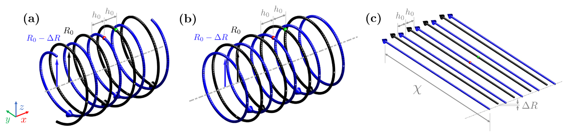
Figure C1 Schematic diagrams depicting the configurations of the vortex filament method tested. The vortex filaments are used to represent the tip vortex system of an asymmetric rotor having a length difference ΔR between the two blades. All these configurations repeat themselves infinitely in both the positive and negative streamwise directions (the direction of the dashed lines in gray). The direction of the circulation Γ is labeled with arrows, and all the filaments have Γ of equal strength. (a) The system with helical vortex filaments. (b) The system with vortex rings. (c) The system with straight vortex filaments, with χ being the filaments' length.

To determine how δh and δr evolve over time, the trajectories of the red (inner) and green (outer) points shown in Fig. C1 are computed based on the induced velocities acting on them. The corresponding symmetry conditions, either helical symmetry or axial symmetry, and periodicity are applied to allow the values of δh and δr to be derived from the trajectories of these two points. Notably, in the case of helical filaments, the non-zero induced velocity in the y direction, v_in, is addressed by applying a correction to the x-directional induced velocity. This correction is made by defining $u_{\text{in, corr}}=u_{\text{in}}+v_{\text{in}}{h}_{\mathrm{0}}/\left(\mathit{\pi }{R}^{\prime }\right)$, where R^′ is the radius of the helix at that time instant. This approach ensures that the y positions of the two points remain unchanged.

The numerical setups for the vortex filament configurations are summarized in this paragraph. For all four configurations, 100 pairs of inner and outer vortex filaments are placed on both sides of the evaluation points (the red and green dots in Fig. C1). Each turn of the helices and each vortex ring is discretized into 100 straight filament segments. The vortex core size is assumed to be infinitesimally small, and the induced velocity at the filament center is set to 0, following Eq. (C1). The filament length parameter χ is set to 2000πR₀ to approximate an infinite-length scenario. Regarding the time step size, $\mathrm{\Delta }t=\mathrm{5}\times {\mathrm{10}}^{-\mathrm{3}}{t}_{\text{Hel}}$. A parametric study confirms that doubling these parameters results in negligible changes in both the growth rate and the leapfrogging distance (less than 0.1 % difference).

The trajectories of the inner (red) and outer (green) points in Fig. C1 are obtained using a time integration approach. At each time step, the positions of these points are updated based on the induced velocities calculated from the vortex filaments, providing the instantaneous values of δh and δr. The vortex filaments are then reconstructed according to the updated δh and δr. This process is repeated iteratively as the algorithm advances to the next time step.

The L1 norms, defined as $\left|\right|\mathit{\eta }|{|}_{\mathrm{1}}\equiv |\mathit{\delta }h|+|\mathit{\delta }r|$, predicted by the four different vortex filament configurations for the case with $\mathrm{\Delta }R/R_{\mathrm{0}}=\mathrm{0.1}$ are plotted against time in Fig. C2. As expected, the curve predicted by the configuration of infinitely long vortex filaments exactly matches that of the 2D vortex model described in Sect. 2.5. In Fig. C2, it is evident that the growth rates and leapfrogging times predicted by all four configurations are very similar, indicating that the effects of finite filament length, curvature, and torsion are minimal for the present application. This result is consistent with expectations, given that both the reduced pitch $\widehat{L}\equiv h_{\mathrm{0}}/\mathit{\pi }R$ and the radial perturbation $\mathrm{\Delta }R/R_{\mathrm{0}}$ are relatively small, with values of 0.12 and 0.1, respectively. The analysis by Delbende et al. (2021) similarly shows that for $\widehat{L}<\mathrm{0.3}$ and $\mathrm{\Delta }R/R_{\mathrm{0}}<\mathrm{0.3}$, the dynamics predicted by the 2D vortex model closely resemble those of helical filament systems. Based on the findings in Fig. C2 and this theoretical context, the 2D vortex model described in Sect. 2.5 is considered suitable for the current application. Moreover, because the induced velocities in the 2D vortex model can be expressed in closed algebraic form, it is preferred for its analytical simplicity compared to the filament method.

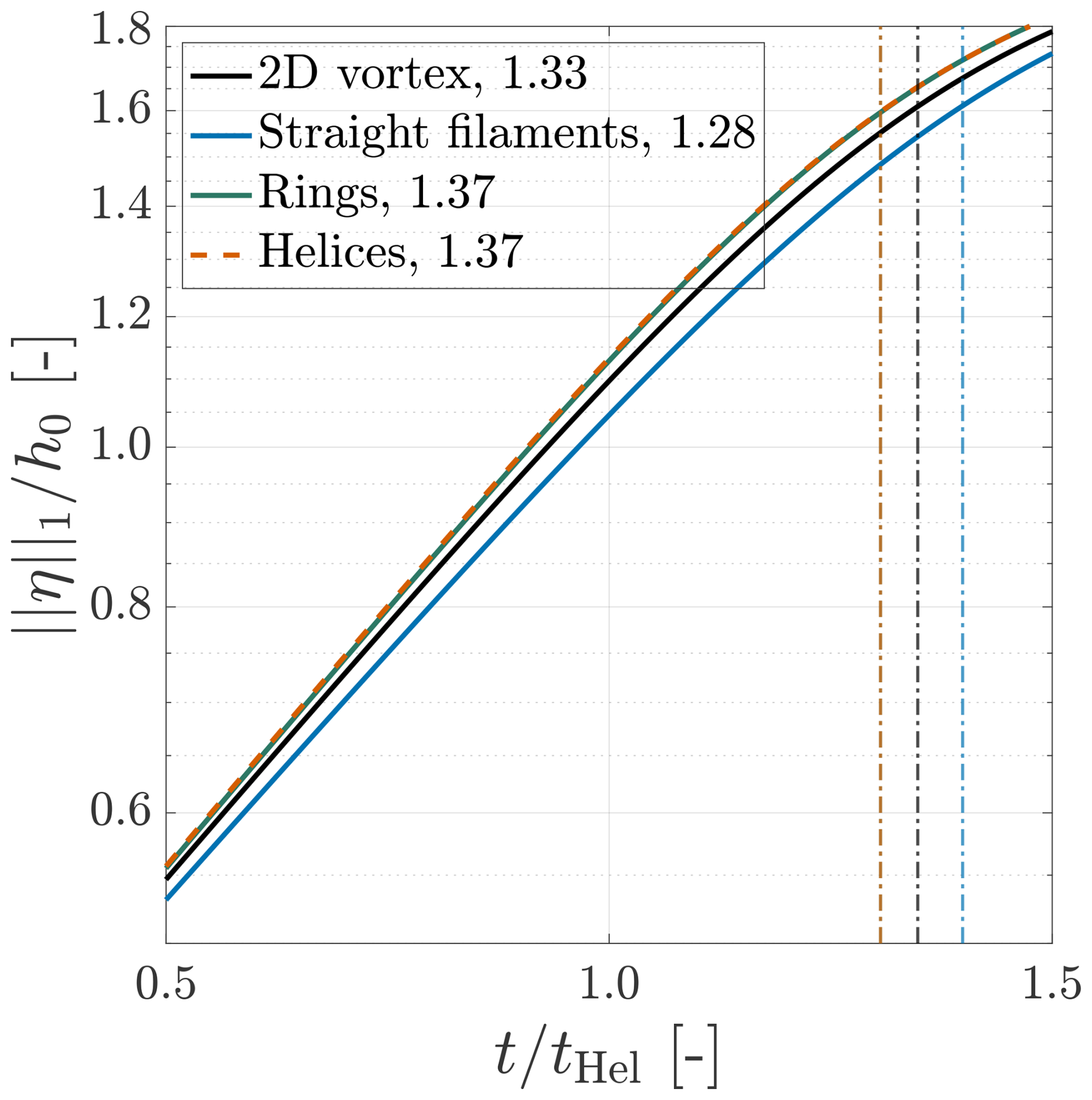
Figure C2 The obtained L1 norm, $\left|\right|\mathit{\eta }|{|}_{\mathrm{1}}=|\mathit{\delta }h|+|\mathit{\delta }r|$, with the four different configurations of vortex filaments depicted in Fig. C1. “2D vortex” is the case when χ in Fig. C1c extends to ∞, whereas “Straight filaments” denotes the configuration with χ=2πR₀. The numbers in the legend indicate the normalized growth rate (growth rate$/t_{\text{Hel}}^{-\mathrm{1}}$) of each configuration. The vertical dashed lines indicate the leapfrogging time t_LF. Note that t_LF for “Rings” is on top of that for “Helices”.

Looking closer into Fig. C2, it can be found that curvature has the largest impact on $\left|\right|\mathit{\eta }|{|}_{\mathrm{1}}$ and the growth rate with the current settings. Also, limiting the length of the straight vortex filaments χ from ∞ to 2πR₀ has noticeable impacts. The former demonstrates that the effects of curvature increase the growth rate. On the other hand, limiting the length of the vortex filaments decreases it. In contrast, the effects of the torsion/inclination angle are almost undetectable, where the growth rate of the configuration with helical vortices is merely 0.2 % lower than that with vortex rings.

Several remarks regarding the additional limitations of using the filament method are provided in this paragraph. First, although helical vortex filaments can capture some three-dimensional effects, the model used here does not account for viscous effects and assumes infinitely small vortex cores. These limitations make the vortex filaments completely non-diffusive and prevent the vortex from merging, which is unphysical in real-world scenarios. Second, all filament configurations employed in this appendix consist of vortex filaments that extend infinitely in the axial direction, which does not reflect the reality of a wind turbine rotor, where vortex arrays terminate at the rotor plane and introduce spatial inhomogeneities in the streamwise direction. Third, the configurations considered do not include root vortices, which are present in actual turbine wakes and can influence vortex dynamics (Selçuk et al., 2017). Lastly, the vortex filament method used here does not incorporate turbulence effects. In this work, these limitations are overcome by employing large-eddy simulations with actuator lines, allowing for the capture of more realistic and physically detailed wake dynamics of an asymmetric rotor.